Autoencoder with Ordered Variance for
Nonlinear Model Identification

Abstract

This paper presents a novel autoencoder with ordered variance (AEO) in which the loss function is modified with a variance regularization term to enforce order in the latent space. Further, the autoencoder is modified using ResNets, which results in a ResNet AEO (RAEO). The paper also illustrates the effectiveness of AEO and RAEO in extracting nonlinear relationships among input variables in an unsupervised setting.

Keywords Autoencoder  $\cdot$ ResNet  $\cdot$ Unsupervised Learning, Nonlinear Model Identification.

1 Introduction

In general, real-world high dimensional data is likely to concentrate in the vicinity of lower dimensional manifolds due to system constraints [1]. This has resulted in the subfield of unsupervised learning known as dimensionality reduction. Two major problems of interest in dimensionality reduction are:

• P1: Feature extraction: where the objective is to extract lower dimensional features that are desired to be ordered in terms of reconstruction error contribution, variance, etc.

• P2: Model extraction: deals with identifying relationships amongst variables of the high-dimensional data set.

In the case that linear relationships exist between the variables of the data set, both P1 and P2 can be simultaneously solved using principal component analysis (PCA) [2, 3, 4]. In PCA, the objective is to find an optimal linear transformation that maps its high-dimensional input vector (unlabeled) to a lower-dimensional latent (feature) space. Even though PCA identifies and eliminates collinearity in the latent space, this ability degrades when the functional dependence in the input variables becomes nonlinear or equivalently the input variables lie in a non-Euclidean manifold. This leads to the introduction of nonlinear dimensionality reduction methods such as autoencoder (AE) [5, 6], principal curve [7], Kernel PCA [8, 9], isomap [10], locally linear embedding [11, 12], laplacian eigenmap [13], diffusion map [14], etc. Amongst these, AEs are popular because of their connection to neural networks and deep learning [15]. AEs use an encoder to transform its high-dimensional input vector (in input space) to a latent vector (in latent space) followed by a a decoder to reconstruct the input vector from the latent vector. The encoder and decoder are usually nonlinear functions represented using neural networks (NNs). AEs can be considered as a nonlinear counterpart of PCA. However, unlike PCA, in AEs, the latent variables are not ordered and uncorrelated. Consequently, determining the optimal size or dimension of the latent space in AE is difficult.

To address these challenges, various modifications of AEs are presented in the literature, which are mostly based on modifying the loss function with different regularization terms. Variational AE is introduced in [16], in which the objective is to enforce a prior distribution in the latent space by modifying the loss function with a variational Bayes term. In sparse AE [17] and k-sparse AE [18], the objective is to have as few non-zero latent variables as possible. Contractive AE [19] and its variants [20, 21] use the norm of the encoder’s Jacobian as a regularization term. Relational AE [22] uses a regularization term based on the covariance matrices of the input and reconstructed input. Neural component analysis [23] is a combination of AE and PCA, which uses an NN as the encoder function and a linear mapping as the decoder function. Orthogonal AE is proposed in [24] in which orthogonality in the latent space is achieved using regularization. In [25], a PCA-AE approach is proposed, which uses a covariance loss term and sequential algorithm based on progressively increasing the size of the latent space. Further, [26] proposes an efficient structuring of the latent space in AEs using Shapley values, which results in ordering based on reconstruction contribution. Deep AEs are introduced in [27], which use deep NNs in the encoder and decoder. Residual networks (ResNets) are proposed in [28], which use residual or skip connections for dealing with the performance degradation issue in deep NNs. Recently, ResNet autoencoder (RAE) and convolutional RAE (CRAE) for image classification are introduced [29], which use ResNets as encoder functions. Even though ordering of latent variables in terms of reconstruction error is achieved in [25, 26], ordering in terms of variances is not achieved in any of the above approaches.

Apart from feature extraction, an important aspect of PCA is that the residual equation in PCA represents a linear equation, and hence, equivalently, provides a linear model between the variables directly from the data set [3, 4]. However, the extension of this idea to nonlinear model identification has not been elucidated. Although authors in [30] presented a kernel principal component regression based nonlinear model identification and data reconciliation, it requires the data to be labeled in the form of input and output variables. Further, in kernel-based methods, the identified models are non-parametric. When it comes to AEs, the problem of model extraction has not been explored in the literature.

To summarize, the ordering of latent variables in terms of variance and nonlinear model identification using AEs are open problems to the best of the authors’ knowledge. This motivates the current work, wherein we attempt to solve both of these open problems. For that, we introduce an autoencoder with ordered variance (AEO), which is then modified using ResNets (RAEO). Further, the paper illustrates the effectiveness of AEO and RAEO in extracting nonlinear relationships among the input variables. Compared to the literature, the contributions in this paper are highlighted below:

1. The proposed AEO and RAEO with regularized loss function result in ordered latent variables in terms of decreasing variance. Here, the ordering is achieved by modifying the loss function with a regularization term containing a non-uniform weighted sum of the latent variable variances.

2. The AEO and RAEO extract nonlinear relationships amongst input variables in implicit form and are thus used for nonlinear model identification. Further, RAEO provides an opportunity to extract explicit nonlinear relationships when dependent variables are user-defined.

The rest of the paper is organized as follows. Section 2 discusses the relevant preliminary concepts from PCA and AE. The proposed AEO approach is presented in Section 3, which also discusses the nonlinear model extraction using AEO with a numerical example. Section 4 presents the extension of AEO with ResNet (RAEO) and its effectiveness in nonlinear model identification. Section 5 illustrates the numerical implementation of AEO and RAEO approaches and the analysis of the simulation results. Finally, conclusions and future directions are discussed in Section 6.

Notations: Scalars are represented by normal font ($A,a$), matrices and vectors by boldface letters ($\textbf{A},\textbf{a}$), and sets by blackboard bold font ($\mathbb{A}$). The $n$ - dimensional Euclidean space is denoted by $\mathbb{R}^{n}$ and the space of $m\times n$ real matrices by $\mathbb{R}^{m\times n}$. The orthogonal complement of a subspace $\mathbb{P}$ is denoted by $\mathbb{P}^{\perp}.$ For a vector $\textbf{x},$ the sample mean vector and sample covariance matrix are denoted by $\bar{\textbf{x}},\textbf{V}_{\textbf{x}},$ respectively. For a matrix $\textbf{A}\in\mathbb{R}^{m\times n},$ the Frobenious norm is denoted as ${\parallel\textbf{A}\parallel}_{F},$ where ${\parallel\textbf{A}\parallel}_{F}=\sqrt{\sum_{i=1}^{m}\sum_{j=1}^{n}a_{ij}^{2}}=\sqrt{Trace(\textbf{A}^{T}\textbf{A})}.$ For $\textbf{A}\in\mathbb{R}^{m\times n},$ the submatrix containing first $p$ rows and $q$ columns is denoted by $\textbf{A}_{[p\times q]}.$ Finally, $\textbf{I}_{n}$ is used to represent identity matrix of order $n\times n.$

2 Preliminaries

2.1 Principal Component Analysis (PCA)

PCA is a dimensionality reduction method and belongs to unsupervised learning algorithms [2, 3]. In PCA, the objective is to linearly transform the input data into a latent space where most of the information or variation in the data can be described with fewer dimensions. Consider the input data:

$$\textbf{X}=\left[\begin{matrix}\textbf{x}_{1}&\textbf{x}_{2}&\dots&\textbf{x}_{N}\end{matrix}\right]$$ (1)

where $\textbf{x}=\textbf{x}_{j}\in\mathbb{R}^{n},$ $j=1,..,N$ are the $N$ samples which are assumed to be mean-centered, and $\textbf{X}\in\mathbb{R}^{n\times N}$. Each sample x consists of measurements of $n$ variables. Dimensionality reduction is achieved in PCA by linearly transforming the input vector to the latent vector:

$$\textbf{y}=\textbf{P}^{T}\textbf{x}$$ (2)

where $\textbf{x}\in\mathbb{R}^{n}$ is the input vector, $\textbf{y}\in\mathbb{R}^{m}$ is the latent vector, $m\leq n,$ and $\textbf{P}\in\mathbb{R}^{n\times m}$ contains $m$ orthonormal columns which are also called principal components. From $\textbf{y},$ the reconstructed input is computed as:

$$\hat{\textbf{x}}=\textbf{P}\textbf{y}=\textbf{P}\textbf{P}^{T}\textbf{x}.$$ (3)

where $\hat{\textbf{x}}\in\mathbb{R}^{n}$ is the reconstructed input vector. We define the latent and reconstructed data as:

$$\textbf{Y}=\left[\begin{matrix}\textbf{y}_{1}&\textbf{y}_{2}&\dots&\textbf{y}_{N}\end{matrix}\right]$$ (4)

$$\hat{\textbf{X}}=\left[\begin{matrix}\hat{\textbf{x}}_{1}&\hat{\textbf{x}}_{2}&\dots&\hat{\textbf{x}}_{N}\end{matrix}\right]$$

where $\textbf{Y}\in\mathbb{R}^{m\times N},\hat{\textbf{X}}\in\mathbb{R}^{n\times N}$ represent $N$ samples of the latent vectors, and reconstructed input vectors, respectively.

Given the input data $\textbf{X},$ the PCA transformation matrix P can be obtained by solving the constrained optimization problem [31]:

$$\underset{\textbf{P}}{\min}\hskip 5.69046pt{\parallel\textbf{X}-\hat{\textbf{X}}\parallel}_{F}^{2}\hskip 25.6073ptor\hskip 22.76228pt\underset{\textbf{P}}{\min}\hskip 5.69046pt{\parallel\textbf{X}-\textbf{P}\textbf{P}^{T}\textbf{X}\parallel}_{F}^{2}$$ (5)

$$\text{subj. to}~{}~{}\textbf{P}^{T}\textbf{P}=\textbf{I}_{m}\hskip 48.36958pt\text{subj. to}\hskip 8.5359pt\textbf{P}^{T}\textbf{P}=\textbf{I}_{m}$$

where the loss function is chosen for minimizing the reconstruction error and the equality constraint is used for obtaining an orthonormal transformation. If the reconstruction error in the objective function in Eq. (5) is negligible, then the identification of the $m$ latent variables from the $n$ input variables with $m<n$ can be interpreted as dimensionality reduction or feature extraction. Further, PCA can also be used for identifying linear relationships amongst the input variables, as discussed next.

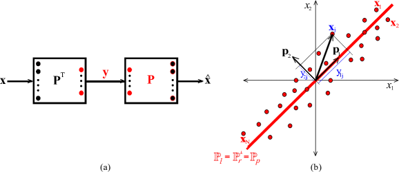
Figure 1: (a) PCA block diagram (b) PCA illustration.

2.2 Linear Model Extraction using PCA

One of the applications of PCA is to identify the linear relationships among the input variables. Such relationships can be identified using latent variables with (nearly) zero variances, known as residual variables [4]. Since the latent variables in PCA are ordered in terms of decreasing variance, the residual variables will correspond to the last few elements of y with zero variance. During model extraction using PCA, we set $m=n.$ Further, we consider that the first $p$ latent variables have nonzero variance (or significant) while the remaining $n-p$ are with zero variance (or residual). Thus, the first $p$ principal components are treated as significant and the rest $n-p$ as residual components, i.e., $\textbf{P}=\left[\begin{matrix}\textbf{P}_{p}&\textbf{P}_{r}\end{matrix}\right]$ where $\textbf{P}_{p}\in\mathbb{R}^{n\times p}$ and $\textbf{P}_{r}\in\mathbb{R}^{n\times(n-p)}.$ Based on this, the latent variables can be partitioned into:

$$\textbf{y}=\left[\begin{matrix}\textbf{y}_{p}\\ \textbf{y}_{r}\end{matrix}\right]=\left[\begin{matrix}\textbf{P}_{p}^{T}\\ \textbf{P}_{r}^{T}\end{matrix}\right]\textbf{x}$$ (6)

where $\textbf{y}_{p}\in\mathbb{P}_{p},$ $\textbf{y}_{r}\in\mathbb{P}_{r}$ contain the significant and residual variables, and $\mathbb{P}_{p},\mathbb{P}_{r}$ are subspaces of $\mathbb{R}^{n}$ with dimension $n$ and $n-p,$ respectively. The residual variables have zero mean and zero variance, which implies $\textbf{y}_{r}=0.$ Substituting this in Eq. (6) results in:

$$\textbf{P}_{r}^{T}\textbf{x}=\textbf{0}$$ (7)

which gives a linear model containing $n-p$ relationships amongst the input variables. In general, any set of $n-p$ variables in x corresponding to linearly independent columns in $\textbf{P}_{r}$ can be solved using the above equation, given the remaining $p$ variables in $\textbf{x}.$ We denote the subspace containing all the vectors satisfying Eq. (7) as $\mathbb{P}_{l}$. In PCA, the principal components are orthogonal which implies $\mathbb{P}_{p}=\mathbb{P}_{r}^{\perp}.$ Further, Eq. (7) results in:

$$\mathbb{P}_{l}=\mathbb{P}_{r}^{\perp}=\mathbb{P}_{p}$$ (8)

In practice, the input data contains measurement noise and outliers. Consequently, the elements of $\textbf{y}_{r}$ can be defined as the latent variables with $V_{y_{i}}<\epsilon$ where $V_{y_{i}}$ is the variance of the latent variable $y_{i}$ and $\epsilon>0$ is a tolerance value. This is illustrated in Fig. 1(b), where it can be observed that most of the data is oriented along $\textbf{p}_{1}$ and the variance of the data in the direction of $\textbf{p}_{2}$ is small, i.e., $V_{y_{2}}$ is on account of measurement noise and can be neglected. Further, since the data is mean-centered (centered around the origin in Fig. 1(b)), the mean $\bar{\textbf{x}}=0\implies\bar{y}_{2}=0.$ This results in:

$$y_{2}=\textbf{p}_{2}^{T}\textbf{x}=0$$ (9)

which gives a linear model as in Eq. (7) where $\mathbb{P}_{p}=span(\{\textbf{p}_{1}\})$ and $\mathbb{P}_{r}=span(\{\textbf{p}_{2}\})$. Next, we discuss the AE as a nonlinear extension of the PCA.

2.3 Autoencoder (AE)

AEs come under unsupervised learning and are used for efficient low-dimensional representation of unlabeled data [5, 6]. AEs can be considered as two sequentially connected NNs that are trained together using the unlabelled input data X (see Fig. 2(a)). The first NN is called the encoder, which maps the input vector into a (possibly) low-dimensional space. The second NN or decoder reconstructs the input vector from its low-dimensional representation. The encoder and decoder can be mathematically represented as:

$$\textbf{y}=\textbf{e}(\textbf{x})$$ (10)

$$\hat{\textbf{x}}=\textbf{d}(\textbf{y})=\textbf{d}(\textbf{e}(\textbf{x}))$$

where $\textbf{x}\in\mathbb{R}^{n}$ is the input vector, $\textbf{y}\in\mathbb{R}^{m}$ is the encoded vector or latent vector, $\hat{\textbf{x}}\in\mathbb{R}^{n}$ is the reconstructed input vector, $\textbf{e}:\mathbb{R}^{n}\rightarrow\mathbb{R}^{m}$ is the encoder function, and $\textbf{d}:\mathbb{R}^{m}\rightarrow\mathbb{R}^{n}$ is the decoder function. In general, $m\leq n,$ whereas, in the case of dimensionality reduction, $m<n.$

In AEs, the objective is to find the encoder and decoder functions that result in the reconstructed vector $\hat{\textbf{x}}$ such that the reconstruction error is minimized. This results in the unconstrained optimization problem for AE [23]:

$$\underset{\textbf{e},\textbf{d}}{\min}\hskip 5.69046pt{\parallel\textbf{X}-\hat{\textbf{X}}\parallel}_{F}^{2}\hskip 19.91684ptor\hskip 19.91684pt\underset{\textbf{e},\textbf{d}}{\min}\hskip 5.69046pt{\parallel\textbf{X}-\textbf{d}(\textbf{e}(\textbf{X})\parallel}_{F}^{2}.$$ (11)

AEs can be considered as nonlinear extensions of PCA in which the linear transformations in Eqs. (2) and (3) are replaced by nonlinear functions in Eq. (10). This is illustrated in Fig. 2(a). Generally, AEs are suitable for datasets containing nonlinear relationships amongst input variables as in Fig. 2(b).

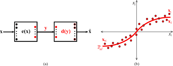
Figure 2: (a) AE block diagram (b) AE illustration.

Several variants of AEs have been proposed in the literature. Linear autoencoders (LAEs), which use linear activation functions are studied in [31, 32, 33]. In LAEs, the encoder and decoder functions are linear: $\textbf{e}(\textbf{x})=\textbf{W}_{1}\textbf{x}$ and $\textbf{d}(\textbf{y})=\textbf{W}_{2}\textbf{y}$ where $\textbf{W}_{1}\in\mathbb{R}^{m\times n},\textbf{W}_{2}\in\mathbb{R}^{n\times m}.$ Consequently, with suitable regularization [32] the weights in LAE can learn the principal components: $\textbf{W}_{1}=\textbf{P}^{T}$ and $\textbf{W}_{2}=\textbf{P}$. In [34], a PCA-boosted AE approach is presented, which uses the PCA solution as the initial condition for AE. In nonlinear PCA using AEs, the encoder and decoder are nonlinear functions such as NNs with nonlinear activation functions [5, 35]. Generally, AEs (or PCA) can be implemented either sequentially or simultaneously [5]. The loss function for simultaneous AE based on Eq. (11) is:

$$J={\parallel\textbf{X}-\hat{\textbf{X}}\parallel}_{F}^{2}={\parallel\textbf{X}-\textbf{d}(\textbf{e}(\textbf{X}))\parallel}_{F}^{2}$$ (12)

where weights and biases for encoder and decoder functions are computed by optimizing the loss function. In sequential AE [5], a series of $m$ networks containing a single latent variable are trained. The residual from the $i^{th}$ network becomes the input for the $(i+1)^{th}$ network resulting in:

$$\textbf{Y}_{i}=\textbf{e}_{i}(\textbf{X}_{i})$$ (13)

$$\textbf{X}_{i+1}=\textbf{X}_{i}-\hat{\textbf{X}}_{i}=\textbf{X}_{i}-\textbf{d}_{i}(\textbf{Y}_{i})$$

where $\textbf{X}_{i}\in\mathbb{R}^{n\times N},$ $\textbf{Y}_{i}\in\mathbb{R}^{1\times N},\hat{\textbf{X}}_{i}\in\mathbb{R}^{n\times N},$ $i=1,2,...,m$ and $\textbf{X}_{1}=\textbf{X}.$ Even though sequential PCA identifies latent variables with ordered variance, the same cannot be ensured in the sequential AE. However, there exist a few approaches that ensure ordering in the latent space of AE in terms of reconstruction error [25, 26]. In PCA-AE[25], a regularization term with the covariance matrix $\textbf{V}_{\textbf{y}}$ of the latent vector is included in the loss function:

$$J={\parallel\textbf{X}-\hat{\textbf{X}}\parallel}_{F}^{2}+\alpha{\parallel\textbf{V}_{\textbf{y}}\parallel}_{F}^{2},\hskip 28.45274pt\alpha>0$$ (14)

using which the AE is trained sequentially. Similarly, in relational AE [22], the relationship amongst the variables (in terms of covariances) is incorporated into the loss function as a regularization term. Apart from this, orthogonal AE modifies the loss function as [24]:

$$J={\parallel\textbf{X}-\hat{\textbf{X}}\parallel}_{F}^{2}+\alpha{\parallel\textbf{Y}^{T}\textbf{Y}-\textbf{I}_{N}\parallel}_{F}^{2},\hskip 14.22636pt\alpha>0$$ (15)

which imposes orthogonality on the learned representation in the latent space. However, none of the above approaches achieve the ordering of latent variables in terms of variance.

The extension of AEs in the direction of manifold learning is studied in contractive AE [19] and its variants [20, 21]. The motivation behind manifold learning is the unsupervised learning hypothesis [1], which states that real-world data in high dimensional spaces is likely to concentrate in the vicinity of a lower dimensional non-linear manifold. Manifold learning is achieved in contractive AE by modifying the loss function as [19]:

$$J={\parallel\textbf{X}-\hat{\textbf{X}}\parallel}_{F}^{2}+\alpha{\parallel\nabla_{\textbf{x}}\textbf{y}\parallel}_{F}^{2},\hskip 14.22636pt\alpha>0$$ (16)

where the encoder’s Jacobian $\nabla_{\textbf{x}}\textbf{y}$ is the gradient of y with respect to $\textbf{x}.$ Here, the regularization term forces the latent variables to be constant, i.e., the gradient with respect to the input variables to be nearly zero. Generally, the manifold learning algorithms [10]-[12] are used for learning a function that transforms the input vector into a lower-dimensional manifold in the latent space. The extension of these methods in the direction of model extraction is not explored in the literature. In summary, the use of AEs has primarily been restricted to feature extraction. The notion of order is also limited to the identification of dominant features in terms of reconstruction error. To the best of the authors’ knowledge, no attempt has been made in the literature to extract nonlinear relationships using AEs (analogous to PCA).

These motivate the current work where the main objectives are: 1. Ordering of latent variables in terms of variance, 2. Nonlinear model identification using AEs. In the next section, we present the autoencoder with ordered variance (AEO) which can achieve the above objectives.

3 Autoencoder with Ordered variance (AEO)

In this section, we propose the AEO in which the loss function is modified with a variance regularization term to enforce order in the latent space. The encoder and decoder functions for the AEO are chosen as NNs, which results in the latent and reconstructed vectors:

$$\textbf{y}=\textbf{e}_{\textbf{NN}}(\textbf{x})=\textbf{f}_{E}(\textbf{f}_{E-1}(...(\textbf{f}_{1}(\textbf{x}))))$$ (17)

$$\hat{\textbf{x}}=\textbf{d}_{\textbf{NN}}(\textbf{y})=\textbf{f}_{E+D}(\textbf{f}_{E+D-1}(...(\textbf{f}_{E+1}(\textbf{y}))))$$

where $\textbf{x}\in\mathbb{R}^{n},\textbf{y}\in\mathbb{R}^{m},$ $\textbf{f}_{1},...,\textbf{f}_{E}$ are layers of the encoder, $\textbf{f}_{E+1},...,\textbf{f}_{E+D}$ are layers of the decoder, $E$ and $D$ are the number of layers in the encoder and decoder, respectively. Let the input and output of the $i^{th}$ layer be denoted by $\textbf{u}_{i}$ and $\textbf{v}_{i}.$ Then, each layer $\textbf{f}_{i}$ can be represented as:

$$\textbf{v}_{i}=\textbf{f}_{i}(\textbf{u}_{i})=\bm{\sigma}_{i}(\textbf{A}_{i}\textbf{u}_{i}+\textbf{b}_{i})$$ (18)

where $\bm{\sigma}_{i}={\left[\begin{matrix}\sigma_{i_{1}}\\ \vdots\\ \sigma_{i_{m_{i}}}\end{matrix}\right]}$ contains the element-wise activation functions for the $i^{th}$ layer, $m_{i}$ is the number of neurons in $i^{th}$ layer, $\textbf{A}_{i}\in\mathbb{R}^{m_{i}\times m_{i-1}}$ is the weight matrix, $\textbf{b}_{i}\in\mathbb{R}^{m_{i}}$ is the bias vector, $\textbf{v}_{i}\in\mathbb{R}^{m_{i}},$ $\textbf{u}_{i}\in\mathbb{R}^{m_{i-1}},$ $i=1,2,..E+D$, $m_{0}=n,m_{E}=m,$ $m_{E+D}=n,$ $\textbf{u}_{1}=\textbf{x},\textbf{v}_{E}=\textbf{y},$ and $\textbf{v}_{E+D}=\hat{\textbf{x}}$ .

Let A contain the weights and biases for all layers in the encoder and decoder. Now, the loss function for the AEO is defined as:

$$J={\underbrace{\alpha{\parallel\textbf{X}-\hat{\textbf{X}}\parallel}_{F}^{2}}_{J_{1}}+\underbrace{\beta{\parallel\textbf{Q}^{\frac{1}{2}}[\textbf{Y}-\bar{\textbf{Y}}]\parallel}_{F}^{2}}_{J_{2}}+\underbrace{\gamma{\parallel\textbf{A}\parallel}_{F}^{2}}_{J_{3}}}$$ (19)

where $\bar{\textbf{Y}}=\left[\begin{matrix}\bar{\textbf{y}}&\bar{\textbf{y}}&\dots&\bar{\textbf{y}}\end{matrix}\right]\in\mathbb{R}^{m\times N}$ contains the mean latent vector $\bar{\textbf{y}}$ as its elements, $\alpha,\beta,\gamma>0$ are the tuning parameters, and $\textbf{Q}=diag(q_{1},q_{2},...,q_{m})$ is the weighting matrix. The elements of Q are chosen as $0\leq q_{1}<q_{2}<...<q_{m}<\infty$ so that the latent variables can be ordered in terms of decreasing variance. Here, the loss function consists of three components:

1. Reconstruction error term $J_{1}$: denotes the sum of square error between the given data and reconstructed data.

2. Variance regularization term $J_{2}$: is used for ordering the latent variables in terms of their variances $V_{y_{i}},$ i.e., $J_{2}=\beta\hskip 2.84544ptTrace([\textbf{Y}-\bar{\textbf{Y}}]^{T}\textbf{Q}[\textbf{Y}-\bar{\textbf{Y}}])=\beta(N-1)(q_{1}V_{y_{1}}+...+q_{m}V_{y_{m}}).$

3. Weight regularization term $J_{3}$: is used for avoiding overfitting and large weights (mostly in decoders).

Now, the optimization problem for AEO becomes:

$$\underset{\textbf{A}}{\min}\hskip 5.69046ptJ$$ (20)

where $J$ is the loss function in Eq. (19).

We have seen that PCA can be used for extracting a lower dimensional linear model as in Eq. (7) directly from data. An analogous approach to extract a nonlinear model using AEO is presented next.

3.1 Extracting Nonlinear Relationships using AEO

In this section, the application of AEO in nonlinear model identification is discussed. As discussed in the context of PCA, the latent variables with $V_{y_{i}}<\epsilon$ are identified using AEO, and the nonlinear relationship in the manifold $\mathbb{P}_{nl}$ is extracted. For that, the AEO with $m=n$ is considered, which is trained using the available input data to identify those latent variables $y_{i},$ $i=p+1,...,n$ whose variance $V_{y_{i}}<\epsilon$. Without loss of generality, we assume the input data is mean-centered, and the bias terms are chosen as zero. Further, the activation function for the encoder and decoder output layers: $\bm{\sigma}_{E}$ and $\bm{\sigma}_{E+D}$ are chosen as linear. This simplifies y and $\hat{\textbf{x}}$ in Eq. (17) as:

$$\textbf{y}=\textbf{A}_{E}\bm{\sigma}_{E-1}(\textbf{A}_{E-1}...\bm{\sigma}_{1}(\textbf{A}_{1}\textbf{x}))$$ (21)

$$\hat{\textbf{x}}=\textbf{A}_{E+D}\bm{\sigma}_{E+D-1}(\textbf{A}_{E+D-1}...\bm{\sigma}_{1}(\textbf{A}_{E+1}\textbf{y})).$$

Since the variance of latent variables in AEO is ordered, the latent variables from $p+1$ to $n$ can be considered to have zero variance. Then, the elements in y and $\textbf{A}_{E}$ can be grouped as follows:

$${\textbf{y}=\left[\begin{matrix}\textbf{y}_{p}\\ \textbf{y}_{r}\end{matrix}\right]},\hskip 5.69046pt{\textbf{A}_{E}=\left[\begin{matrix}\textbf{A}_{E_{p}}\\ \textbf{A}_{E_{r}}\end{matrix}\right]}$$ (22)

where $\textbf{y}_{p}\in\mathbb{R}^{p},\textbf{y}_{r}\in\mathbb{R}^{n-p},\textbf{A}_{E_{p}}\in\mathbb{R}^{p\times m_{E-1}},$ $\textbf{A}_{E_{r}}\in\mathbb{R}^{(n-p)\times m_{E-1}}.$ Using these, the latent vector in Eq. (21) can be rewritten as:

$$\textbf{y}=\left[\begin{matrix}\textbf{y}_{p}\\ \textbf{y}_{r}\end{matrix}\right]=\left[\begin{matrix}\textbf{A}_{E_{p}}\\ \textbf{A}_{E_{r}}\end{matrix}\right]\bm{\sigma}_{E-1}(\textbf{A}_{E-1}...\bm{\sigma}_{1}(\textbf{A}_{1}\textbf{x})).$$ (23)

Now, $\textbf{V}_{\textbf{y}_{r}}=\textbf{0}$ implies $\textbf{y}_{r}=\bar{\textbf{y}}_{r},$ which results in:

$$\textbf{A}_{E_{r}}\bm{\sigma}_{E-1}(\textbf{A}_{E-1}...\bm{\sigma}_{1}(\textbf{A}_{1}\textbf{x}))-\bar{\textbf{y}}_{r}=\textbf{0}.$$ (24)

The above equation gives $n-p$ nonlinear relationships among the variables in x in implicit form. Given an appropriate set of $p$ variables in $\textbf{x},$ one can solve Eq. (24) for the remaining $n-p$ variables using numerical solvers for nonlinear system of equations [36]. The solutions of the above equation define a $p$ - dimensional nonlinear manifold $\mathbb{P}_{nl}$ in $\mathbb{R}^{n}.$ The model identification using AEO is illustrated next with an example.

3.2 Illustrating AEO

To illustrate AEO, a dataset $\{\textbf{x}_{1},...,\textbf{x}_{100}\}$ containing 100 samples of a 2D vector $\textbf{x}={\left[\begin{matrix}x_{1}\\ x_{2}\end{matrix}\right]}$ is considered. Let $x_{1}$ and $x_{2}$ be related by the nonlinear equation:

$$x_{2}-tanh(3\hskip 1.42271ptx_{1})=0.$$ (25)

To generate the data, 100 samples of $x_{1}$ are selected as uniformly distributed random variables with mean zero. The samples for $x_{2}$ are generated from $x_{1}$ using Eq. (25). The data is then normalized and used as the input in AEO. The encoder and decoder functions for AEO are selected using Eq. (21) with $n=2,$ $m=2,$ $E=2,D=2,$ $m_{1}=5,m_{3}=5,$ and $\bm{\sigma}=\textbf{tanh}.$ The model parameters are stored in the matrix A and the optimization problem in Eq. (20) is solved for A using Quasi-Newton method. The loss function parameters are chosen as $\alpha=1,$ $\beta=0.5,$ $\gamma=0.1,$ $\textbf{Q}=diag(1,q^{2})$ with $q$ varying from 1 to 10 for which the results are plotted in Fig. 3. The variances of latent variables $y_{1},$ $y_{2}$ with respect to $q$ are shown in Fig. 3(a). It can observed that the ordering is achieved for $q\geq 2$. Further, $V_{y_{2}}=0$ for $q\geq 4$ with $\bar{y}_{2}=0$. The plot of $J_{1},J_{2},J_{3}$ with respect to $q$ is given in Fig. 3(b).

Now, an implicit relationship between the variables $x_{2}$ and $x_{1}$ can obtained by substituting $\textbf{A}_{1},$ $\textbf{A}_{2_{r}},$ and $\bar{y}_{2}$ for $q=10$ in Eq. (24) which gives:

$${{\left[\begin{matrix}0.036\\ -0.084\\ 0.089\\ 0.031\\ -0.093\end{matrix}\right]^{T}}}\textbf{tanh}\bigg{(}{{\left[\begin{matrix}0.062&0.283\\ 0.173&0.208\\ -0.123&0.044\\ 0.149&-0.118\\ -0.188&-0.083\end{matrix}\right]}}{\left[\begin{matrix}x_{1}\\ x_{2}\end{matrix}\right]}\bigg{)}=0.$$ (26)

The above equation is solved for $x_{2}$ with actual $x_{1}$ using the trust-region-dogleg algorithm in which the actual values of $x_{1}$ are substituted and the equation is solved for $x_{2}.$ The estimation of $x_{2}$ obtained by solving the implicit relationship in Eq. (26) is denoted by $x_{fim_{2}}$. The top panel in Fig. 3(c) shows the plot of $x_{1}$ vs $x_{2}$ and $x_{1}$ vs $x_{fim_{2}}$ for $q=10$. The bottom panel in Fig. 3(c) shows the mean square error (MSE) between $x_{2}$ and $x_{fim_{2}}$ which becomes approximately zero for $q=10$, i.e. $x_{fim_{2}}\approx x_{2}.$

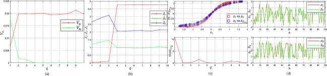
Figure 3: Response of 2-variable example with AEO.

Remark 1.

The advantages and potential applications of AEO are listed below:

1. AEO does not require a sequential implementation to achieve ordering, i.e., ordering is achieved with simultaneous training where all the nodes in the bottleneck layer are trained together. Ordering of latent variables has applications in the following areas:

   • Dimensionality reduction: where ordering helps in determining the optimal size or dimension of the latent space.

   • Image classification: where ordering helps in prioritizing different features in an image.

2. AEO is successful in identifying the nonlinear relationship with sufficient accuracy. Identifying nonlinear models from data has applications in the following areas:

   • Data reconciliation [30]: where models can be used for identifying faulty sensors, improving the sensor data or noisy measurements.

   • Soft sensing[37]: where models can be used for estimating non-measurable variables from noisy measurements.

   • Process monitoring[38, 39]: where models can be used to improve fault detection and diagnosis performance.

   • Real-time optimization[40]: where models are used to specify process operating constraints.

Remark 2.

Even though AEO can extract nonlinear relationships, its performance depends on the parameters $\alpha,\beta,\gamma$ and $\textbf{Q},$ which need to be tuned properly. Apart from this, AEO has the following shortcomings:

1. It is observed that AEO can result in the trivial solution $\textbf{A}_{E_{r}}=\textbf{0},$ $\bar{\textbf{y}}_{r}=\textbf{0}$ (Eq. (24)) and in that case identifying the nonlinear relationships is not possible. One way to avoid this issue is to add constraints on $\textbf{A}_{E_{r}}$ such as ${\parallel\textbf{A}_{E_{r}}\parallel}_{F}^{2}=1$ and retrain AEO.

2. The nonlinear relationship obtained from AEO is in implicit form. Even though such relationships can be solved numerically using various solvers, their accuracy depends on the initial conditions, uniqueness of solutions, etc. Further, obtaining an explicit relationship is beneficial in real-time applications such as soft sensing, data reconciliation, etc.

This motivates the extension of AEO, and in the next section, we propose the ResNet autoencoder with ordered variance (RAEO) in which a ResNet is used as encoder and decoder functions. RAEO can extract an explicit relationship between the input variables which will be illustrated using a numerical example.

4 ResNet Autoencoder with Ordered variance (RAEO)

Residual neural networks or residual networks (ResNets) are neural networks that have a residual connection or skip connection, as shown in Fig. 4. Two commonly used forms of ResNet functions are [28]:

1. ResNet with a direct skip connection, denoted as $\textbf{f}_{\textbf{RN}}:$

   $$\textbf{y}=\textbf{f}_{\textbf{RN}}(\textbf{x})=\textbf{x}+\textbf{f}_{\textbf{NN}}(\textbf{x})$$ (27)

   where $\textbf{x}\in\mathbb{R}^{n},\textbf{y}\in\mathbb{R}^{m},$ $\textbf{f}_{\textbf{NN}}:\mathbb{R}^{n}\rightarrow\mathbb{R}^{m},$ and $m=n.$

2. ResNet with a weighted skip connection (weighted ResNet), denoted as $\textbf{f}_{\textbf{WRN}}:$

   $$\textbf{y}=\textbf{f}_{\textbf{WRN}}(\textbf{x})=\textbf{A}_{\textbf{R}}\textbf{x}+\textbf{f}_{\textbf{NN}}(\textbf{x})$$ (28)

   where $\textbf{x}\in\mathbb{R}^{n},\textbf{y}\in\mathbb{R}^{m},$ $\textbf{A}_{\textbf{R}}\in\mathbb{R}^{m\times n},$ $\textbf{f}_{\textbf{NN}}:\mathbb{R}^{n}\rightarrow\mathbb{R}^{m},$ and $m\leq n.$

In the proposed RAEO, the encoder and decoder functions are selected as weighted ResNets (Fig. 5). Here $\textbf{e}_{\textbf{WRN}},\textbf{d}_{\textbf{WRN}}$ stands for encoder and decoder functions with weighted ResNet. This gives y and $\hat{\textbf{x}}$ for RAEO as:

y $$=\textbf{e}_{\textbf{WRN}}(\textbf{x})=\textbf{A}_{\textbf{e}}\textbf{x}+\textbf{e}_{\textbf{NN}}(\textbf{x})$$ (29)

$$=\textbf{A}_{\textbf{e}}\textbf{x}+\textbf{f}_{E}(\textbf{f}_{E-1}(...(\textbf{f}_{1}(\textbf{x}))))$$

$$\hat{\textbf{x}} =\textbf{d}_{\textbf{WRN}}(\textbf{y})=\textbf{A}_{\textbf{d}}\textbf{y}+\textbf{d}_{\textbf{NN}}(\textbf{y})$$

$$=\textbf{A}_{\textbf{d}}\textbf{y}+\textbf{f}_{E+D}(\textbf{f}_{E+D-1}(...(\textbf{f}_{E+1}(\textbf{y}))))$$

where $\textbf{x}\in\mathbb{R}^{n},\textbf{y}\in\mathbb{R}^{m},$ $\textbf{A}_{\textbf{e}}\in\mathbb{R}^{m\times n}$ and $\textbf{A}_{\textbf{d}}\in\mathbb{R}^{n\times m}$. In this paper we consider $\textbf{A}_{e}$ and $\textbf{A}_{d}$ as fixed (user specified) parameters. The loss function for the RAEO is chosen as in Eq. (19). Now, the optimization problem for RAEO can be defined as in Eq. (20).

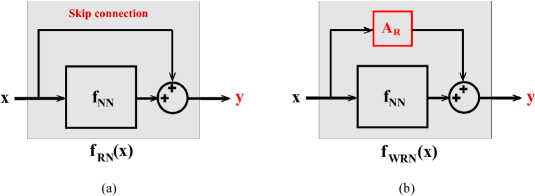
Figure 4: (a) ResNet (b) Weighted ResNet.

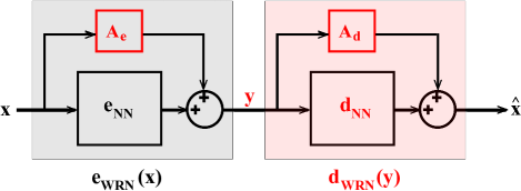
Figure 5: ResNet Autoencoder.

The weighted ResNet [28] in Fig. 4(b) can be considered as a generalized ResNet, which leads to the following special cases:

1. $\textbf{f}_{\textbf{NN}}$: for which $\textbf{A}_{\textbf{R}}=\textbf{0}.$

2. $\textbf{f}_{\textbf{RN}}$: for which $\textbf{A}_{\textbf{R}}=\textbf{I}_{[m\times n]}.$

3. $\textbf{f}_{\textbf{PCA-RN}}$: for which $\textbf{A}_{\textbf{R}}=\textbf{P}_{[m\times n]}^{T}$ where $\textbf{P}^{T}$ comes from the PCA.

4. $\textbf{f}_{\textbf{WRN}}$: for which $\textbf{A}_{\textbf{R}}$ is a trainable parameter.

Now, in RAEO, the encoder and decoder functions can be chosen in the form of any of the above four functions. This leads to 16 variants of RAEO, which are named as RAEO 1-1, RAEO 1-2,…, RAEO 4-4. Out of these 16 combinations, the following two versions are investigated in this paper.

1. RAEO 1-1: for which $\textbf{A}_{\textbf{e}}=\textbf{0}$, and $\textbf{A}_{\textbf{d}}=\textbf{0}$ and is same as AEO (see Section 3).

2. RAEO 2-1: for which $\textbf{A}_{\textbf{e}}=\textbf{I}_{[m\times n]}$, and $\textbf{A}_{\textbf{d}}=\textbf{0}$.

The next section discusses the application of RAEO in nonlinear model identification for which version RAEO 2-1 is used.

4.1 Extracting Nonlinear Relationships using RAEO

Here, we are interested in identifying nonlinear relationships among the input variables. For that, RAEO is trained with the available input data to find the variables in y with zero variance. Similar to AEO, we assume the input data is mean-centered, and the bias terms are chosen as zero. This simplifies y and $\hat{\textbf{x}}$ for RAEO as:

$$\textbf{y}=\textbf{x}+\textbf{A}_{E}\bm{\sigma}_{E-1}(\textbf{A}_{E-1}...\bm{\sigma}_{1}(\textbf{A}_{1}\textbf{x}))$$ (30)

$$\hat{\textbf{x}}=\textbf{y}+\textbf{A}_{E+D}\bm{\sigma}_{E+D-1}(\textbf{A}_{E+D-1}...\bm{\sigma}_{1}(\textbf{A}_{E+1}\textbf{y})).$$

Let the variables from $p+1$ to $n$ have zero variance. Then elements in y and $\textbf{A}_{E}$ can grouped as in Eq. (22). Further, the elements in x and $\textbf{A}_{1}$ are grouped as:

$$\textbf{x}=\left[\begin{matrix}\textbf{x}_{p}\\ \textbf{x}_{r}\end{matrix}\right],\hskip 14.22636pt\textbf{A}_{1}=\left[\begin{matrix}\textbf{A}_{1_{p}}&\textbf{A}_{1_{r}}\end{matrix}\right]$$ (31)

where $\textbf{x}_{p}\in\mathbb{R}^{p},\textbf{x}_{r}\in\mathbb{R}^{n-p},\textbf{A}_{1_{p}}\in\mathbb{R}^{m_{1}\times p},$ $\textbf{A}_{1_{r}}\in\mathbb{R}^{m_{1}\times(n-p)}.$ Using this, Eq. (29) can be rewritten as:

y $$={\left[\begin{matrix}\textbf{y}_{p}\\ \textbf{y}_{r}\end{matrix}\right]=\textbf{x}+\textbf{A}_{E}\bm{\sigma}_{E-1}(\textbf{A}_{E-1}...\bm{\sigma}_{1}(\textbf{A}_{1}\textbf{x}))}$$ (32)

$$={\left[\begin{matrix}\textbf{x}_{p}\\ \textbf{x}_{r}\end{matrix}\right]+\left[\begin{matrix}\textbf{A}_{E_{p}}\\ \textbf{A}_{E_{r}}\end{matrix}\right]\bm{\sigma}_{E-1}(\textbf{A}_{E-1}...\bm{\sigma}_{1}(\textbf{A}_{1_{p}}\textbf{x}_{p}+\textbf{A}_{1_{r}}\textbf{x}_{r}))}.$$

Now, $\textbf{V}_{\textbf{y}_{r}=\textbf{0}}$ results in:

$$\textbf{x}_{r}+\textbf{A}_{E_{r}}\bm{\sigma}_{E-1}(\textbf{A}_{E-1}...\bm{\sigma}_{1}(\textbf{A}_{1_{p}}\textbf{x}_{p}+\textbf{A}_{1_{r}}\textbf{x}_{r}))-\bar{\textbf{y}}_{r}=\textbf{0}$$ (33)

which represents an implicit relationship among input variables. Further, in the case of RAEO, it is possible to obtain an explicit relationship as well where the objective is to represent $\textbf{x}_{r}$ as a nonlinear function of $\textbf{x}_{p}.$ For that, select $\textbf{A}_{1_{r}}=\textbf{0}$ and retrain the RAEO to make $\textbf{V}_{\textbf{y}_{r}}=\textbf{0}$ which modifies Eq. (33) to an explicit relationship between $\textbf{x}_{r}$ and $\textbf{x}_{p}$ as:

$$\textbf{x}_{r}=\bar{\textbf{y}}_{r}-\textbf{A}_{E_{r}}\bm{\sigma}_{E-1}(\textbf{A}_{E-1}...\bm{\sigma}_{1}(\textbf{A}_{1_{p}}\textbf{x}_{p})).$$ (34)

Here, one can also use other versions: RAEO 3-3, RAEO 4-4, etc, and derive relationships similar to Eq. (34).

Remark 3.

The advantages of RAEO in comparison with AEO are as follows:

1. The ResNet makes it easier to extract nonlinear relationships in explicit form. However, the success of getting an explicit relation cannot be guaranteed, i.e., achieving $\textbf{V}_{\textbf{y}_{r}}=\textbf{0}$ with the constraint $\textbf{A}_{1_{r}}=0$ may not be possible always. In such cases, one can rearrange the variables in x (so that the last $n-p$ variables can represented as a function of the first $p$ variables) and retrain RAEO.

2. The skip connection in RAEO avoids the trivial solutions of zero weights. This can be observed from Eq. (33) where $\textbf{x}_{r}$ comes from the input data which makes $\textbf{x}_{r}\neq 0,$ in practice. Consequently, the trivial solution $\textbf{A}_{E_{r}}=\textbf{0},$ $\bar{\textbf{y}}_{r}=0$ is avoided.

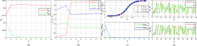
Figure 6: Response of 2-variable example with RAEO.

4.2 Illustrating RAEO

To illustrate RAEO, the example from Section 3.2 is considered again. The data is generated using Eq. (25) as in Section 3.2 which is then normalized and given to the RAEO. The encoder and decoder functions for the RAEO are chosen as in (29) with $n=2$, $m=2,$ $E=2,D=2$, $m_{1}=5,$ $m_{3}=5,$ $\textbf{A}_{\textbf{e}}=\textbf{I},$ and $\textbf{A}_{\textbf{d}}=\textbf{0}$. Parameters for the loss function are chosen as $\alpha=1,$ $\beta=0.5,$ $\gamma=0.1,$ $\textbf{Q}=diag(1,q^{2})$ and $q$ is varied from 1 to 10 for which the results are plotted in Fig. 6.

The variance of the elements in y is plotted against $q$ in Fig. 6(a), which shows the variance of $y_{2}$ becomes zero for $q=4$ onwards. This indicates that with a value of $q\geq 4,$ the variance $V_{y_{2}}=0.$ The plot of the terms $J_{1},J_{2},J_{3}$ with respect to $q$ is given in Fig. 6(b).

Now with RAEO, an implicit relationship among the input variables can be obtained by substituting $\textbf{A}_{1},$ $\textbf{A}_{2_{r}},$ and $\bar{y}_{2}$ for $q=10$ in Eq. (33) which gives:

$$x_{2}+ {{\left[\begin{matrix}-0.814\\ -0.676\\ -0.727\\ -0.909\\ 0.453\end{matrix}\right]^{T}}}\textbf{tanh}\bigg{(}{{\left[\begin{matrix}0.054&0.318\\ -0.588&0.641\\ 0.119&0.231\\ 0.241&0.112\\ -0.312&-0.010\end{matrix}\right]}}{\left[\begin{matrix}x_{1}\\ x_{2}\end{matrix}\right]}\bigg{)}=0.$$ (35)

Moreover, in the case of RAEO, an explicit relationship can be obtained by substituting $\bar{y}_{2},$ $\textbf{A}_{2_{r}},\textbf{A}_{1_{p}}$ in Eq. (34) which results in:

$$x_{2}=- {{\left[\begin{matrix}-1.183\\ 0.037\\ -0.037\\ 0.037\\ 0.037\end{matrix}\right]^{T}}}\textbf{tanh}\bigg{(}{{\left[\begin{matrix}1.753\\ -0.352\\ 0.352\\ -0.352\\ -0.352\end{matrix}\right]x_{1}}}\bigg{)}.$$ (36)

In practice, recovering the exact relationship is difficult. However, an equivalent nonlinear function can be obtained that characterizes the relationships among the variables. The estimation of $x_{2}$ obtained from the implicit relationship in Eq. (35) and the explicit relationship in Eq. (36) are denoted by $x_{fim_{2}}$ and $x_{fex_{2}},$ respectively. The top panel in Fig. 6(c) shows the plot of $x_{1}$ vs $x_{2},$ $x_{1}$ vs $x_{fex_{2}}$ and $x_{1}$ vs $x_{fim_{2}}$ for $q=10.$ The bottom panel in Fig. 6(c) shows the MSE between $x_{2}$ and $x_{fim_{2}}$ which becomes approximately zero from $q=2$ onwards. The top panel also shows the predicted data using the explicit relationship Eq. (36), which is denoted by $x_{fex_{2}}$ and is plotted in green color. Further, the MSE between $x_{2}$ and $x_{fex_{2}}$ is shown in the bottom panel, which is very small. Finally, Fig. 6(d) shows the plot of actual input and reconstructed input for $q=10$ where we can see that the reconstruction is sufficiently accurate. Next, the proposed methods are implemented on a realistic dataset containing more variables and noise.

5 Simulation Results

This section illustrates the proposed methods on a 5-variable dataset: $x_{1},x_{2},x_{3},$ $x_{4},x_{5}$. The variables are related by the following nonlinear equations:

$$x_{4}-sin(3x_{1})=0$$ (37)

$$x_{5}-x_{2}+tan(0.5x_{3})=0.$$

To generate the data, $N=300$ samples of $x_{1},x_{2},x_{3}$ are selected, which are chosen as uniform random variables with zero mean. From this, the samples for $x_{4}$ and $x_{5}$ are generated using Eq. (37) to which Gaussian noise with zero mean and variance of $0.1$ is added. The data is then normalized and used as the input in AEO and RAEO. The tuning parameters of AEO and RAEO are chosen by trial and error for the best results in terms of model identification accuracy. The parameters for AEO are chosen as $E=2,D=2,$ $m_{1}=6,m_{3}=6,$ $\alpha=0.2,$ $\beta=0.3,$ $\gamma=0.08,$ and for RAEO $E=2,D=2,$ $m_{1}=5,m_{3}=5,$ $\alpha=0.3,$ $\beta=0.1,$ $\gamma=0.12$. The weighting matrices for AEO and RAEO are chosen as $\textbf{Q}=diag(0.1,0.1q,0.5q,4q,5q)$ and $q$ is varied from 1 to 10. The results for AEO and RAEO are plotted in Figs. 7 and 8, respectively. Figs. 7(a) and 8(a) show the variances of latent variables with respect to $q.$ It is observed that the ordering is achieved for $q\geq 2$. The plot of the terms $J_{1},J_{2},J_{3}$ with respect to $q$ is given in Figs. 7(b) and 8(b). Further, Figs. 7(c) and 8(c) shows the plot of the actual data: $x_{1}$ vs $x_{4},$ and the predicted data $x_{1}$vs $x_{fim_{4}}$ for $q=10.$ Finally, Figs. 7(d) and 8(d) shows the time series plot of the actual data: $x_{1},x_{4}$ and reconstructed data: $\hat{x}_{1},\hat{x}_{4}$ which shows the reconstruction is sufficiently accurate. Table I shows the performance comparison of AEO and RAEO with PCA in which the MSE of prediction error ($mse(x_{4}-x_{fim_{4}})$) and reconstruction error ($mse(x_{4}-\hat{x}_{4})$) are compared. The simulation results lead to the following observations:

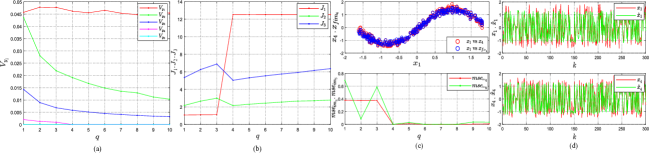
Figure 7: Response of 5-variable example with AEO.

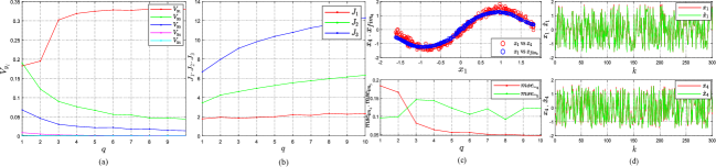
Figure 8: Response of 5-variable example with RAEO.

1. The performance of AEO and RAEO depends on the parameters: $\alpha,$ $\beta,$ $\gamma,$ Q, and the number of samples $N.$ In general, the number of samples required to extract an accurate model depends on the complexity of the nonlinearity.

2. From Figs. 6(d) and 7(d), it is observed that RAEO results in smaller values of reconstruction error compared to AEO.

3. In Table I, the prediction error is large for PCA, which indicates that the linear model identified with PCA is not sufficient for predicting $x_{4}.$ Whereas the prediction error is small for both AEO and RAEO which indicates that the identified models with AEO and RAEO are sufficiently accurate.

Method	$mse(x_{4}-x_{fim_{4}})$	$mse(x_{4}-\hat{x}_{4})$
PCA	0.9967	0.0966
AEO	0.0064	0.0966
RAEO	0.0476	0.0060

Table 1: Performance comparison.

6 Conclusions

This paper proposed an autoencoder with an ordered variance of latent variables (AEO), which is then modified using ResNets (RAEO). The performance of AEO and RAEO are compared using various numerical simulations. The simulation results show that AEO and RAEO are useful for nonlinear model identification in an unsupervised setting. The future works are designing an algorithm for finding the optimal tuning parameters ($\alpha,\beta,\gamma,\textbf{Q}$), obtaining theoretical guarantees on model identification accuracy, and exploring other versions of RAEO.

References

- [1] L. Cayton, “Algorithms for Manifold Learning,” Technical Report CS2008-0923, University of California, Jun. 2005.
- [2] K. Pearson, “On Lines and Planes of Closest Fit to Systems of Points in Space,” Philosophical Magazine, vol. 2, pp. 559-572, 1901.
- [3] J. Jackson, “A User’s Guide to Principal Components,” Wiley, New York, Mar. 1991.
- [4] S. Narasimhan and S. Shah, “Model Identification and Error Covariance Matrix Estimation from Noisy Data using PCA,” Control Engineering Practice, vol. 16, pp. 146–155, Jan. 2008.
- [5] M. Kramer, “Nonlinear Principal Component Analysis Using Autoassociative Neural Networks,” AIChE Journal, vol. 37, pp. 233-243, Feb. 1991.
- [6] P. Baldi and K. Hornik, “Neural Networks and Principal Component Analysis: Learning from Examples Without Local Minima,” Neural Networks, vol. 2, pp. 53-58, 1989.
- [7] T. Hastie and W. Stuetzle,“Principal Curves,” Journal of the American Statistical Association, vol. 84, pp. 502-516, Jun. 1989.
- [8] B. Scholkopf, A. Smola, and K. Muller, “Nonlinear Component Analysis as a Kernel Eigenvalue Problem,” Neural Computation, vol. 10, pp. 1299–1319, Jul. 1998.
- [9] J. Ham, D. Lee, S. Mika, B. Scholkopf, “A Kernel view of the Dimensionality Reduction of Manifolds,” Proceedings of the 21st International Conference on Machine Learning, Banff, Canada, Jul. 2004.
- [10] J. Tenenbaum, L. de Silva, “A Global Geometric Framework for Nonlinear Dimensionality Reduction,” Science, vol. 290, pp. 2319–2323, Dec. 2000.
- [11] S. Roweis, L. Saul, “Nonlinear Dimensionality Reduction by Locally Linear Embedding,” Science, vol. 290, pp. 2323–2326, Dec. 2000.
- [12] L. Saul and S. Roweis, “Think Globally, Fit Locally: Unsupervised Learning of Low dimensional Manifolds,” Journal of Machine Learning Research, vol. 4, pp. 119–155, Jun. 2003.
- [13] M. Belkin and P. Niyogi, “Laplacian Eigenmaps and Spectral Techniques for Embedding and Clustering,” Proceedings of the Conference on Neural Information Processing Systems, Vancouver, Canada, Dec. 2001.
- [14] B. Nadler, S. Lafon, R. Coifman, I. Kevrekidis, “Diffusion maps, Spectral clustering, and Eigenfunctions of Fokker–Planck Operators,” Proceedings of the Conference on Neural Information Processing Systems, Vancouver, Canada, Dec. 2005.
- [15] P. Li, Y. Pei, and J. Li, “A Comprehensive Survey on Design and Application of Autoencoder in Deep Learning,” Applied Soft Computing, vol. 138, pp. 1-21, May 2023.
- [16] D. Kingma, and M. Welling, “Auto-Encoding Variational Bayes,” Proceedings of the International Conference on Learning Representations, Banff, Canada, Apr. 2014.
- [17] H. Lee, c. Ekanadham, and A. Ng, “Sparse Deep Belief net Model for Visual area V2,” Proceedings of the Conference on Neural Information Processing Systems, Vancouver, Canada, Dec. 2007.
- [18] A Makhzani and B. Frey, “k-Sparse Autoencoders,” Proceedings of the International Conference on Learning Representations, Banff, Canada, Apr. 2014.
- [19] S. Rifai, P. Vincent, X. Muller, X. Glorot, and Y. Bengio, “Contractive Auto-Encoders: Explicit Invariance During Feature Extraction,” Proceedings of the 28th International Conference on Machine Learning, Bellevue, WA, USA, Jun. 2011.
- [20] S. Rifai, Y. Dauphin, P. Vincent, Y. Bengio, and X. Muller, “The Manifold Tangent Classifier,” Proceedings of the Conference on Neural Information Processing Systems, Granada, Spain, Dec. 2011.
- [21] R. Takhanov, Y. Abylkairov, and M. Tezekbayev, “Autoencoders for a Manifold Learning Problem with a Jacobian Rank Constraint,” Pattern Recognition, vol. 143, pp. 1-11, Jun. 2023.
- [22] Q. Meng, D. Catchpoole, D. Skillicom, P. Kennedy, “Relational Autoencoder for Feature Extraction,” Proceedings of the International Joint Conference on Neural Networks (IJCNN), Anchorage, USA, May 2017.
- [23] H. Zhao,“Neural Component Analysis for Fault Detection,” Chemometrics and Intelligent Laboratory Systems, vol. 76, pp. 11-21, May 2018.
- [24] W. Wang, D. Yang, F. Chen, Y. Pang, S. Huang, and Y. Ge, “Clustering With Orthogonal AutoEncoder,” IEEE Access, vol. 7, pp. 62421-62432, May 2019.
- [25] C. Pham, S. Ladjal, and A. Newson, “PCA-AE: Principal Component Analysis - Autoencoder for Organising the Latent Space of Generative Networks,” Journal of Mathematical Imaging and Vision, vol. 64, pp. 569–585, Apr. 2022.
- [26] E. Trunz, M. Weinmann, S. Merzbach, R. Klein, “Efficient Structuring of the Latent Space for Controllable Data Reconstruction and Compression,” Graphics and Visual Computing, vol. 7, pp. 1-13, Dec. 2022.
- [27] G. Hinton and R. Salakhutdinov, “Reducing the Dimensionality of Data with Neural Networks,” Science, vol. 73, pp. 504-507, Jul. 2006.
- [28] K. He, X. Zhang, S. Ren, and J. Sunu, “Deep Residual Learning for Image Recognition,” Proceedings of the IEEE Conference on Computer Vision and Pattern Recognition, pp. 770-778, Jun. 2016.
- [29] C. Wickramasinghe, D. Marino, and M. Manic, “ResNet Autoencoders for Unsupervised Feature Learning From High-Dimensional Data: Deep Models Resistant to Performance Degradation,” IEEE Access, vol. 9, pp. 40511-40520, Mar. 2021.
- [30] K. Marimuthu and S. Narasimhan, “Nonlinear Model Identification and Data Reconciliation Using Kernel Principal Component Regression,” Industrial and Engineering Chemistry Research, vol. 58, pp. 11224-11233, May 2019.
- [31] E. Plaut, “From Principal Subspaces to Principal Components with Linear Autoencoders,” Arxiv, https://arxiv.org/pdf/1804.10253.pdf, Dec. 2018.
- [32] D. Kunin, J. Bloom, A. Goeva, and C. Seed, “Loss Landscapes of Regularized Linear Autoencoders,” Proceedings of the International Conference on Machine Learning, California, U.S.A, Jun. 2019.
- [33] X. Bao, J. Lucas, S. Sachdeva, R. Grosse, “Regularized Linear Autoencoders Recover the Principal Components, Eventually,” Proceedings of the Conference on Neural Information Processing Systems, Vancouver, Canada, Dec. 2020.
- [34] M. Digeil, Y. Grinberg, D. Melati, M. Dezfouli, J. Schmid, P. Cheben, S. Janz, and D. Xu, “PCA-Boosted Autoencoders for Nonlinear Dimensionality Reduction in Low Data Regimes,” Arxiv, https://arxiv.org/pdf/2205.11673.pdf, May 2022.
- [35] U. Kruger, J. Zhang, and L. Xie, “Developments and Applications of Nonlinear Principal Component Analysis - a Review,” Principal Manifolds for Data Visualization and Dimension Reduction, Springer, vol 58., pp. 1-43, 2008.
- [36] D. Benton,“Nonlinear Equations: Numerical Methods for Solving,” Amazon Digital Services LLC - Kdp Print Us, Jul. 2018.
- [37] C. Shang, F. Yang, D. Huang, and W. Lyu, “Data-driven Soft sensor Development based on Deep Learning Technique,” Journal of Process Control, vol. 24, pp. 223–233, Feb. 2014.
- [38] J. Lee, C. Yoo, S. Choi, P. Vanrolleghem, and I. Lee, “Nonlinear Process Monitoring using Kernel Principal Component Analysis,” Chemical Engineering Science, vol. 59, pp. 223 – 234, Jan. 2004.
- [39] Z. Li, L. Tian, Q. Jiang, and X. Yan, “Dynamic Nonlinear Process Monitoring based on Dynamic Correlation Variable Selection and Kernel Principal Component Regression,” Journal of the Franklin Institute, vol. 359, pp. 4513-4539, Jun. 2022.
- [40] J. Trierweiler, “Real-Time Optimization of Industrial Processes,” Encyclopedia of Systems and Control, pp. 1 – 11, Jan. 2014.