Practical Kernel Tests of Conditional Independence

Abstract

We describe a data-efficient, kernel-based approach to statistical testing of conditional independence. A major challenge of conditional independence testing, absent in tests of unconditional independence, is to obtain the correct test level (the specified upper bound on the rate of false positives), while still attaining competitive test power. Excess false positives arise due to bias in the test statistic, which is obtained using nonparametric kernel ridge regression. We propose three methods for bias control to correct the test level, based on data splitting, auxiliary data, and (where possible) simpler function classes. We show these combined strategies are effective both for synthetic and real-world data.

1 Introduction

Conditional independence (CI) testing is a fundamental problem in statistics: given a confounder $Z$, are two random variables $X$ and $Y$ dependent? Applications include basic scientific questions (“is money associated with self-reported happiness, controlling for socioeconomic status?”); evaluating the fairness of machine learning methods (the popular equalized odds criterion (Mehrabi et al., 2021) checks that predictions are independent of a protected status, given the true label); causal discovery (where conditional independence testing is a core sub-routine of many causal structure discovery methods, building on the PC algorithm; Spirtes et al., 2000; Pearl, 2000; Sun et al., 2007; Tillman et al., 2009), and more. If $Z$ takes on a small number of discrete values and sufficient data points are available, the problem can be essentially reduced to marginal independence testing. In many cases, however, $Z$ takes on continuous values and/or has complex structure; it is then a major challenge to determine how to “share information” across similar values of $Z$, without making strong assumptions about the form of dependence among the variables.

In simple settings, for instance if $(X,Y,Z)$ are jointly Gaussian, conditional independence can be characterized by the partial correlation between $X$ and $Y$ given $Z$, the correlation between residuals of linear regressions $Z\to X$ and $Z\to Y$.

One family of CI tests extends this insight to nonlinear analogues of partial correlation, allowing the detection of nonlinear dependencies, as suggested by the general characterization of conditional independence of Daudin (1980). We consider the Kernel-based Conditional Independence (KCI, Zhang et al., 2011) statistic, and its successor, the Conditional Independence Regression CovariancE (CIRCE, Pogodin et al., 2022) (see Section 3). These methods replace the residuals of linear regression with a kernel analogue, (infinite-dimensional) conditional feature mean estimation (Song et al., 2009; Grünewälder et al., 2012; Li et al., 2022b); they then use a kernel-based alternative to covariance (the Hilbert-Schmidt norm of feature covariance, Gretton et al., 2005, 2007) to detect dependence between these residuals. With appropriate choice of kernels, these methods can (eventually) detect any conditional dependence, not just correlation.

In low-data regimes, however, these methods suffer from some severe practical issues in constructing valid statistical tests. In particular, nonparametric regression for conditional feature means suffers unavoidably from bias (Li et al., 2022b). This bias can easily create dependence between estimated residuals whose population counterparts are independent, dramatically inflating the rate of false positives above the design value for the test. Bias control is therefore essential in minimizing this effect, and controlling the rate of false positives.

The key to our approach may be understood by comparing KCI with CIRCE, keeping in mind that both are zero only at conditional independence. The KCI is a covariance of residuals, and thus two regressions are needed in order to compute it (regression from $Z$ to $X$, and from $Z$ to $Y$). CIRCE, by contrast, requires only regression from $Z$ to $Y$, and computes the covariance of this residual with $X$ alone. In other words, the second regression in KCI, from $Z$ to $X$, is not necessary for consistency of the test – both statistics are zero in population only at conditional independence. Where there is no true signal (at CI) and the regressions are independent, however, it is natural to expect that residuals from a regression to $X$ may “appear less dependent” than $X$ itself, debiasing the overall test (as formalized in Section 4). Thus, even imperfect $Z\rightarrow X$ regression can reduce bias of the test statistic, and improve the Type I error (false detection rate), without compromising test consistency.

This observation gives rise to our first strategy for controlling bias, which is to maximize the accuracy of the regression from $Z$ to $Y$, while enforcing less stringent requirements on the debiasing term from $Z$ to $X$. One route towards the former goal is to use additional auxiliary observations of $(Z,Y)$, if available, since increasing the accuracy of the $Z\rightarrow Y$ regression will greatly reduce test bias. Regarding the latter goal, we may use “smaller” feature spaces for the $Z$ to $X$ regression. These will permit more data-efficient regression — by incorporating prior knowledge, and/or through a finite feature space on $Z$ leading to parametric rates for $Z\rightarrow X$ — without compromising the consistency of the test (which is assured by consistent regression from $Z$ to $Y$). An additional, complementary bias control strategy is to use data splitting, reducing bias accumulation when combining multiple regression estimates.

We call the resulting modification to the KCI and CIRCE family SplitKCI. Employing the wild bootstrap (Wu, 1986; Shao, 2010; Leucht and Neumann, 2013; Chwialkowski et al., 2014) and recent results on conditional mean estimation (Li et al., 2022b), we prove that SplitKCI estimation is much less biased, and further demonstrate greatly improved performance on a variety of empirical settings (Section 5).

Testing terminology. The null hypothesis (denoted $\mathrm{H}_{0}$) is $\mathrm{H}_{0}:X\perp\!\!\!\perp Y\,|\,Z$, i.e. that $X$ is independent of $Y$ given $Z$. The alternative is $\mathrm{H}_{1}:X\mathchoice{\mathrel{\hbox to0.0pt{\kern 7.77777pt\kern-5.27776pt$\displaystyle\not$\hss}{\perp\!\!\!\perp}}}{\mathrel{\hbox to0.0pt{\kern 7.77777pt\kern-5.27776pt$\textstyle\not$\hss}{\perp\!\!\!\perp}}}{\mathrel{\hbox to0.0pt{\kern 2.75006pt\kern-4.11108pt$\scriptstyle\not$\hss}{\perp\!\!\!\perp}}}{\mathrel{\hbox to0.0pt{\kern 1.25006pt\kern-3.3333pt$\scriptscriptstyle\not$\hss}{\perp\!\!\!\perp}}}Y\,|\,Z$. False positives, i.e. rejecting the null when it holds, are called Type I errors. False negatives, i.e. failing to reject the null when the alternative holds, are called Type II errors. Test power is the true positive rate, i.e. 1 minus the Type II error.

2 Related work

Uniformly valid conditional independence test (with correctly controlled false positive rate) do not exist (Shah and Peters, 2020). To make the testing problem well-defined, various methods make (often implicit) assumptions on the underlying class of distributions: that is, they work for a restricted set of nulls and alternatives.

Kernel-based statistics (Sun et al., 2007; Fukumizu et al., 2007; Strobl et al., 2019; Park and Muandet, 2020; Huang et al., 2022; Scetbon et al., 2022), guarantee asymptotic power and control over false positive rate. They rely on conditional mean embedding (CME) estimation, however, which suffers from a slow convergence rate (Li et al., 2022b). As we will see in this paper, this bias will increase Type I error at finite samples.

As an alternative to kernel-based tests, one can assume some dependence or noise structure in the problem to develop a test with better Type I error control, but without guarantees on test power if the assumptions are violated. One such example is the Generalised Covariance Measure (GCM, Shah and Peters, 2020), which assumes additive noise (see also weighted GCM, Scheidegger et al., 2022, and kernelized GCM, Fernández and Rivera, 2022). It is often straightforward, however, to construct distributions that break these assumptions.

Another class of tests considers local permutations based on clusters of the conditioning variable $Z$ (Fukumizu et al., 2007; Sen et al., 2017; Neykov et al., 2021). This is done to simulate the null and compare it to the test data. However, test power in such approaches is sensitive to the marginal distribution of the conditioning variable $Z$ (Kim et al., 2022).

Finally, there are methods (e.g. Candes et al., 2018; Berrett et al., 2020) that rely on sampling from $P(Y\,|\,Z)$ to produce accurate, theoretically justified $p$-values for any measure of conditional dependence. In practice, however, this distribution must be approximated, introducing error.

The overall space of tests of conditional independence introduces a trade-off between simple tests with good Type I error; and richer tests with poor Type I error for finite samples, but broader-ranging asymptotic Type II error guarantees. Kernel-based methods belong to the latter group, but this work pushes them closer to the former one.

3 Kernel-based measures of conditional dependence

We first provide characterization of conditional independence; we then use this to define our conditional dependence measures.

Definition 1 (Daudin, 1980).

Random variables $X$ and $Y$ are independent conditioned on $Z$, denoted $X\perp\!\!\!\perp Y\,|\,Z$, if

$$\mathbb{E}\left[g(X,Z)\,h(Y,Z)\,|\,Z\right]=\mathbb{E}\left[g(X,Z)\,|\,Z\right]\,\mathbb{E}\left[h(Y,Z)\,|\,Z\right]$$

$Z$-almost surely, for all functions $g\in L^{2}_{XZ}$ and $h\in L^{2}_{YZ}$.

Theorem 1 (Daudin, 1980).

$X\perp\!\!\!\perp Y\,|\,Z$ if and only if

$$\mathbb{E}\left[g(X,Z)\,h(Y,Z)\right]=0\quad\forall g\in E_{1},\,h\in E_{2}\,,$$ (1)

where we use $E_{1}=\{g\in L^{2}_{XZ}:\mathbb{E}\left[g(X,Z)\,|\,Z\right]=0\}$ and $E_{2}=\{h\,\in L^{2}_{YZ}:\mathbb{E}\left[h(Y,Z)\,|\,Z\right]=0\}$.

Also, $X\perp\!\!\!\perp Y\,|\,Z$ if and only if

$$\mathbb{E}\left[g(X)\,h(Y,Z)\right]=0\quad\forall g\in E_{1}^{\prime},\,h\in E_{2},$$ (2)

where $E_{1}^{\prime}=\{g\in L^{2}_{X}:\mathbb{E}\left[g(X)\mid Z\right]=0\}$.

Finally, $X\!\perp\!\!\!\perp\!Y\,|\,Z$ iff (2) holds for all $g\in L^{2}_{X}$ and $h\in E_{2}$.

To use this definition in practice, we turn to kernel methods. A kernel $k:\mathcal{X}\times\mathcal{X}\rightarrow\mathbb{R}$ is a function such that $k(x,x^{\prime})=\left<\phi(x),\,\phi(x^{\prime})\right>_{\mathcal{H}_{x}}$, where $\phi:\mathcal{X}\to\mathcal{H}_{x}$ and $\mathcal{H}_{x}$ is a reproducing kernel Hilbert space (RKHS) of functions $f:\mathcal{X}\rightarrow\mathbb{R}$. The reproducing property of $\mathcal{H}_{x}$ states that for any $f\in\mathcal{H}_{x}$, we have $\left<\phi(x),\,f\right>_{\mathcal{H}_{x}}=f(x)$.

$L^{2}$-universal kernels, such as the Gaussian kernel $k(x,x^{\prime})=\exp(-\|x-x^{\prime}\|^{2}/(2\sigma^{2}))$, have their RKHS dense in $L^{2}$ (Sriperumbudur et al., 2011). Such kernels allow us to transform conditional independence properties based on $L^{2}$ functions into kernel-based expressions.

For two separable RKHS $\mathcal{H}_{x}$ and $\mathcal{H}_{y}$, we can define a space (see e.g. Gretton, 2013) of Hilbert-Schmidt operators $A,B:\mathcal{H}_{x}\rightarrow\mathcal{H}_{y}$, denoted $\mathrm{HS}(\mathcal{H}_{x},\mathcal{H}_{y})$, through the inner product

$$\left<A,\,B\right>_{\mathrm{HS}(\mathcal{H}_{x},\mathcal{H}_{y})}^{2}=\sum_{i\in I}\left<Ag_{i},\,Bg_{i}\right>_{\mathcal{H}_{y}}^{2}\,,$$

where $\{g_{i}\}_{i\in I}$ is an orthonormal basis of $\mathcal{H}_{x}$. As a special case, we have the outer products $\phi_{y}\otimes\phi_{x}\in\mathrm{HS}(\mathcal{H}_{x},\mathcal{H}_{y})$, such that for $f\in\mathcal{H}_{x}$, $(\phi_{y}\otimes\phi_{x})f=\left<\phi_{x},\,f\right>_{\mathcal{H}_{x}}\phi_{y}$ and $\left<A,\,\phi_{y}\otimes\phi_{x}\right>_{\mathrm{HS}}=\left<\phi_{y},\,A\phi_{x}\right>_{\mathcal{H}_{y}}$. We will often shorten $\mathrm{HS}(\mathcal{H}_{x},\mathcal{H}_{y})$ to $\mathrm{HS}$ or $\mathrm{HS}_{xy}$.

Using the space of HS operators, we can define covariance operators (Fukumizu et al., 2004). We consider two such measures, in both cases defining $\mu_{X\,|\,Z}(Z)=\mathbb{E}\left[\phi_{x}(X)\,|\,Z\right]$. First, the Kernel-based Conditional Independence (KCI) operator, due to Zhang et al. (2011), is

$$\begin{split}C_{\mathrm{KCI}}=&\,\mathbb{E}\left((\phi_{x}(X)-\mu_{X\,|\,Z}(Z))\otimes\right.\\ &\qquad\left.\phi_{z}(Z)\otimes(\phi_{y}(Y))-\mu_{Y\,|\,Z}(Z))\right)\,.\end{split}$$ (3)

We call this a covariance operator because, for any $f\in\mathcal{H}_{x}$ and $g\in\mathcal{H}_{yz}$ (with a domain of $\mathcal{Y}\times\mathcal{Z}$), $\left<f,\,C_{\mathrm{KCI}}\,g\right>$ is

$$\mathbb{E}\left[\left(f(X)-\mathbb{E}[f(X)|Z]\right)\left(g(Y,Z)-\mathbb{E}[g(Y,Z)|Z]\right)\right]\,.$$

Thus, if $C_{\mathrm{KCI}}=0$, we know that (2) holds for $f\in E_{1}^{\prime}\cap\mathcal{H}_{x}$ and $g\in E_{2}\cap\mathcal{H}_{yz}$. Although $E_{1}^{\prime}$ and $E_{2}$ used by Theorem 1 contain $L^{2}$ functions not in any RKHS, $L^{2}$-universal kernels cover “enough” functions to ensure by continuity that $C_{\mathrm{KCI}}=0$ iff $X\perp\!\!\!\perp Y\,|\,Z$. We can thus test conditional independence by testing if $\lVert C_{\mathrm{KCI}}\rVert_{HS}^{2}=0$.

The Conditional Independence Regression Covariance (CIRCE, Pogodin et al., 2022) operator is

$$C_{\mathrm{CIRCE}}\!=\!\mathbb{E}\bigl{(}\phi_{x}(X)\!\otimes\!\phi_{z}(Z)\!\otimes\!(\phi_{y}(Y))-\mu_{Y|Z}(Z))\bigr{)}.$$ (4)

This corresponds to restricting $g$ in Theorem 1 to $L_{X}^{2}$. CIRCE was introduced to avoid an additional centering step in cases where $\phi_{x}(X)$ is not fixed, e.g. because it is defined through a deep network that is being trained.

When the conditional means are known, the empirical estimators over $n$ points for both measures follow the (quadratic-time) HSIC estimator, with $O(1/\sqrt{n})$ convergence (see, e.g. Pogodin et al., 2022, Corollary C.6):

$$\|C_{\mathrm{KCI}}\|^{2}_{\mathrm{HS}}\approx\frac{1}{n(n-1)}\mathrm{Tr}\,\big{(}HK^{c}_{X}H\left(K_{Z}\odot K_{Y}^{c}\right)\big{)}\,,$$ (5)

where $H=I_{n}-\frac{1}{n}1_{n}1_{n}^{\top}$ is the “centering matrix,”

$$(K^{c}_{X})_{ij}\!=\!\left<\phi_{x}(x_{i})\!-\!\mu_{X\,|\,Z}(z_{i}),\,\phi_{x}(x_{j})\!-\!\mu_{X\,|\,Z}(z_{j})\right>,$$

$K^{c}_{Y}$ is analogous, and $(K_{Z})_{ij}=k_{z}(z_{i},z_{j})$. For CIRCE, $K^{c}_{X}$ is replaced with the non-centered version.

The main challenge in evaluating these measures is in estimating the conditional mean embedding (CME) $\mu_{X\,|\,Z}$ from data. A CME estimator, denoted $\widehat{\mu}_{X\,|\,Z}$, can be constructed from kernel ridge regression (Song et al., 2009; Grünewälder et al., 2012):

$$\widehat{\mu}_{X\,|\,Z}(z)=K_{zZ}(K_{ZZ}+\lambda\,m\,I_{m})^{-1}\Phi_{x}\,,$$ (6)

where if we use $m$ points in estimation, $K_{ZZ}$ is an $m\times m$ matrix, $K_{zZ}$ is $1\times m$, $\Phi_{x}$ is an $m\times\mathcal{H}_{x}$ stack of features, and $\lambda$ is the ridge regression parameter.

The convergence rates of RKHS-valued regression (i.e. going from one RKHS to another) are extensively studied, with Li et al. (2022b) showing that the best-case rate when the target RKHS is universal is $\mathcal{O}\!\left(1/m^{1/4}\right)$ in Hilbert-Schmidt norm, with arbitrarily slow rates for the hardest problems. In cases where $\mu_{X\,|\,Z}$ exists and is known, we would be able to test for independence, but in the worst-case scenario estimating the conditional mean from data can be arbitrarily slow. Even when the regression is smooth enough to get close to $\mathcal{O}\!\left(1/m^{1/4}\right)$ rates, CME estimator convergence might still be too slow in practice. Thus, we must be able to mitigate the bias of CME estimates in our tests.

Other kernel-based measures of conditional dependence (Fukumizu et al., 2007; Strobl et al., 2019; Park and Muandet, 2020; Scetbon et al., 2022) also rely on CME and are limited by CME estimators’s quality. Here we concentrate on KCI-like measures.

4 Reducing CME estimation bias

The CME estimator’s convergence rates imply that orders of magnitudes more (training) data are needed for CME than for the subsequent evaluation of the covariance of residuals. Luckily, if we have separate $(X,Z)$ and/or $(Y,Z)$ pairs in addition to our $(X,Y,Z)$ triples, we can exploit this in the regression. We refer to the $n$ points used for statistic evaluation as $\mathcal{D}_{\mathrm{test}}^{n}$, the $m_{yz}$ points used for estimating $\mu_{Y\,|\,Z}$ as $\mathcal{D}_{\mathrm{train}}^{m_{yz}}$, and the $m_{xz}$ points used for estimating $\mu_{X\,|\,Z}$ as $\mathcal{D}_{\mathrm{train}}^{m_{xz}}$. We always assume the test data is independent of the train data.

In some cases, such as genetic studies (Candes et al., 2018), “unbalanced” $(Y,Z)$ data is available (i.e. $m_{yz}\gg m_{xz}$). In such settings, CIRCE is potentially more suitable for testing since the CME estimate over $(X,Z)$ in KCI would still be poor. We will call this setting the unbalanced data regime, with $m_{yz}\gg m_{xz}$ and independent $\mathcal{D}_{\mathrm{train}}^{m_{yz}}$ and $\mathcal{D}_{\mathrm{train}}^{m_{xz}}$. We will also compare it to the standard regime with $m_{xz}=m_{yz}$ (coming from a joint training set). In both cases we assume we don’t have enough samples to accurately estimate the full $P(Y\,|\,Z)$ distribution. This work is primarily interested in improving performance in the unbalanced regime.

We start by analyzing the effect of an incorrect CME, which introduces an additional bias into our dependence measure (even at population level, $n=\infty$, not only in the empirical estimate). Under $\mathrm{H}_{0}$, for $\widehat{C}_{\mathrm{KCI}}$ defined using $\widehat{\mu}_{X\,|\,Z}(z)=\mu_{X\,|\,Z}(z)+\widehat{b}_{X\,|\,Z}(z)$ and an analogous $\widehat{\mu}_{Y\,|\,Z}$,

$$\widehat{C}_{\mathrm{KCI}}=\mathbb{E}\left((\phi_{x}(X)-\mu_{X\,|\,Z}(Z)-\widehat{b}_{X\,|\,Z}(Z))\otimes\right.$$

$$\qquad\left.\phi_{z}(Z)\otimes(\phi_{y}(Y))-\mu_{Y\,|\,Z}(Z)-\widehat{b}_{Y\,|\,Z}(Z))\right)$$

$$=\mathbb{E}\,(\widehat{b}_{X\,|\,Z}(Z)\otimes\phi_{z}(Z)\otimes\widehat{b}_{Y\,|\,Z}(Z))\,.$$

We therefore have, for independent copies $Z,Z^{\prime}$, that

$$\|\widehat{C}_{\mathrm{KCI}}\|_{\mathrm{HS}}^{2}=\mathbb{E}\Big{(}\left<\widehat{b}_{X\,|\,Z}(Z),\,\widehat{b}_{X\,|\,Z}(Z^{\prime})\right>_{\mathcal{H}_{x}}\\ k_{z}(Z,Z^{\prime})\left<\widehat{b}_{Y\,|\,Z}(Z),\,\widehat{b}_{Y\,|\,Z}(Z^{\prime})\right>_{\mathcal{H}_{y}}\Big{)}.$$

Since we expect $\hat{b}$ to be relatively smooth with respect to $k_{z}$, it is reasonable to expect that when $k_{z}(Z,Z^{\prime})$ is large, the sign of both inner products will also be positive. Thus, if the bias is ignored, the statistic will appear to indicate dependence, even though none exists—potentially leading to drastic Type I error rates. For CIRCE, the $\langle\widehat{b}_{X\,|\,Z}(Z),\,\widehat{b}_{X\,|\,Z}(Z^{\prime})\rangle_{\mathcal{H}_{x}}$ term in the last equation is replaced by $\left<\mu_{X\,|\,Z}(X),\,\mu_{X\,|\,Z}(X^{\prime})\right>_{\mathcal{H}_{x}}$, yielding a potentially large term for the same reasons.

Ideally, we want to remove some of the $Z$ dependence from $\phi_{x}(X)$ to decrease the CIRCE-like term, but de-correlate the estimation bias to reduce the KCI-like term. We can do this by combining KCI and CIRCE measures. This gives a flexible space of asymptotically equivalent measures of conditional independence.

Theorem 2 (SplitKCI).

For any two arbitrary functions $\omega_{x}^{(1)},\omega_{x}^{(2)}\!:\mathcal{Z}\!\rightarrow\!\mathcal{H}_{x}$, define the corresponding HS operators

$$C_{\omega_{x}^{(i)}}=\mathbb{E}\Bigl{(}(\phi_{x}(X)-\omega_{x}^{(i)}(Z))\otimes{}\\ \phi_{z}(Z)\otimes(\phi_{y}(Y)-\mu_{Y\,|\,Z}(Z))\Bigr{)}.$$

Their product $\left<C_{\omega_{x}^{(1)}},\,C_{\omega_{x}^{(2)}}\right>_{\mathrm{HS}}$, called SplitKCI, is zero if $X\perp\!\!\!\perp Y\,|\,Z$ and positive otherwise.

The empirical estimator coincides with the KCI estimator (5), but using $K_{X}^{c}$ defined as

$$(K^{c}_{X})_{ij}=\left<\phi_{x}(x_{i})-\omega_{x}^{(1)}(z_{i}),\,\phi_{x}(x_{j})-\omega_{x}^{(2)}(z_{j})\right>\,.$$

Proof idea.

The proof, in Section A.1, shows equivalence between this measure and KCI. The estimator is then derived with standard tools. In practice, we will symmetrize the measure as $\frac{1}{2}\langle C_{\omega_{x}^{(1)}},\,C_{\omega_{x}^{(2)}}\rangle+\frac{1}{2}\langle C_{\omega_{x}^{(2)}},\,C_{\omega_{x}^{(1)}}\rangle$ to work with symmetric matrices in the code. ∎

A first insight from SplitKCI is to use different train splits for $\omega_{x}^{(1)}$ and $\omega_{x}^{(2)}$, but otherwise still computing the CME. This can be viewed as an estimator of KCI with decreased bias, due to the decorrelation of the $\left<\widehat{\mu}_{X\,|\,Z}(z_{i}),\,\widehat{\mu}_{X\,|\,Z}(z_{j})\right>$ term.

To analyze SplitKCI, we make standard assumptions that guarantee CME estimator’s convergence.

Assumption 1 (CME rates, Fischer and Steinwart, 2020).

(EVD) The eigenvalues $\mu_{i}$ of $C_{ZZ}=\mathbb{E}\left[\phi_{z}(Z)\otimes\phi_{z}(Z)\right]$ decay as $\mu_{i}\leq c_{\mu}\,i^{-1/p}$, for some $c_{\mu}>0$ and $p\in(0,1]$.
(Boundedness) $k_{z}(Z,Z^{\prime})\leq 1$.
(SRC) The conditional mean operators satisfy $\mu_{X\,|\,Z}\in[\mathrm{HS}_{xz}]^{\beta},\mu_{Y\,|\,Z}\in[\mathrm{HS}_{yz}]^{\beta}$ for the same $\beta\in[1,2]$..

The last condition uses an interpolation space $[\mathrm{HS}]^{\beta}$ (Steinwart and Scovel, 2012), which modifies the conditions on eigenvalue convergence of HS spaces. $[\mathrm{HS}]^{1}$ is the original HS space. For $\beta>1$, $[\mathrm{HS}]^{\beta}$ is a subspace of the original space with smoother operators (and, therefore, faster convergence of the estimator). We use the same $\beta$ for both operators for convenience; all proofs apply for different $\beta_{xz},\beta_{yz}$.

Theorem 3 (Bias in KCI and SplitKCI).

Under 1 and using independent data splits $\mathcal{D}_{\mathrm{train}}^{m_{xz}}$ (for KCI), $\mathcal{D}_{\mathrm{train}}^{m_{xz}/2},\mathcal{D}_{\mathrm{train}}^{m_{xz}/2}$ (for SplitKCI), and $\mathcal{D}_{\mathrm{train}}^{m_{yz}}$ (both), the bias for both methods under $\mathrm{H}_{0}$ are bounded as

$$b_{\mathrm{KCI}}\leq((1\!+\!K_{1}))\,\|\mu_{X\,|\,Z}\|_{\beta}^{2}\!+\!K_{2})\,m_{xz}^{-\frac{\beta-1}{\beta+p}}\,K_{3}\,m_{yz}^{-\frac{\beta-1}{\beta+p}}\,,$$

$$b_{\mathrm{SplitKCI}}\leq 2\,\|\mu_{X\,|\,Z}\|_{\beta}^{2}\,m_{xz}^{-\frac{\beta-1}{\beta+p}}\,K_{3}\,m_{yz}^{-\frac{\beta-1}{\beta+p}}\,,$$

where $K_{1}\!=\!5184,K_{2},K_{3}>0$ do not depend on $m_{xz},m_{yz}$, and $\|\cdot\|_{\beta}$ is the interpolation space norm (see Li et al., 2022b).

Proof idea.

The proof, in Section A.2, compares the bias terms using the CME estimator’s rates (Li et al., 2022b). The KCI bound is much larger due to the constants in the upper bounds of the CME estimator – realistically, these constants are unlikely to be tight.

The $b_{\mathrm{KCI}}$ bound is a sum of two terms: one from the bias due to non-zero ridge parameter $\lambda$, $\|\mu_{X\,|\,Z}\|_{\beta}^{2}m_{xz}^{-\frac{\beta-1}{\beta+p}}K_{3}m_{yz}^{-\frac{\beta-1}{\beta+p}}$, and a (much larger due to $K_{1}=5184$) term $(K_{1}\,\|\mu_{X\,|\,Z}\|_{\beta}^{2}+K_{2})m_{xz}^{-\frac{\beta-1}{\beta+p}}K_{3}m_{yz}^{-\frac{\beta-1}{\beta+p}}$, which comes from $\left<\widehat{\mu}_{X\,|\,Z}(z_{i}),\,\widehat{\mu}_{X\,|\,Z}(z_{j})\right>$.

For SplitKCI, the latter term is zero, as we use two independent CME estimators. The former term is doubled, though, since each regression is done with $m_{xz}/2$ points and $2^{\frac{\beta-1}{\beta+p}}<2$. ∎

This change is somewhat counter-intuitive: finding the CME is hard, so we want as much data as we can. But due to the slow scaling with $m_{xz}$, halving the data doesn’t hurt the overall estimate as much as decorrelating the errors improves it.

This result also shows the benefit of auxiliary $(Y,Z)$ data for the kernel-based test: even for SplitKCI, the remaining bias term is still large unless $m_{yz}$ is large.

Our third debiasing approach also makes use of different $\omega^{(1)}_{x}$ and $\omega^{(2)}_{x}$, and follows directly from Theorem 2:

Corollary 3.1.

For $X\,|\,Z$ conditional mean estimation in SplitKCI, $\omega^{(1)}_{x}$ and $\omega^{(2)}_{x}$ can be CME estimators computed with different, not necessarily universal, kernels.

Simple, non-universal kernels may results in faster-converging CME estimators, even though they might not be able to fully remove $Z$ dependence from $\phi_{x}(X)-\omega_{x}(Z)$; for instance, we can set $p=0$ in Theorem 3 for finite-dimensional kernels. Using different kernels might also help with decorrelating errors. This flexibility also allows us to use $Z$ kernels that take into account some properties of the data. For instance, for discrete $X$, we might benefit from a $Z$ kernel constructed from a linear kernel on the outputs of logistic regression (see e.g. Liu et al., 2020, Section 4).

In summary, SplitKCI debiases KCI with three complementary approaches:

• Data splitting for estimating $\mu_{X\,|\,Z}$ significantly reduces estimation bias (Theorem 3).

• Auxiliary data (i.e. large $m_{yz}$) reduces bias further, and guarantees test consistency, similar to estimator convergence for CIRCE Pogodin et al. (2022).

• Non-universal kernels for $\mu_{X\,|\,Z}$ allows the test to be more flexible (e.g. when there’s structure in $Z$) and potentially makes CME estimators converge faster.

4.1 Wild bootstrap for computing p-values

To use KCI-like measures for statistical testing, we need to compute (approximate) $p$-values for the data. This is not straightforward: under the null, these statistics are distributed as an infinite weighted sum of chi-squared variables (Fernández and Rivera, 2022), rather than a Gaussian (as often the case with other statistics). This distribution does not have a closed form density, and so has to be approximated. The original KCI paper used a Gamma approximation (Zhang et al., 2011), which lacks strict guarantees. In our preliminary experiments, this approximation did not produce correct $p$-values (Figure 6 in the Appendix), so we turn to the wild bootstrap approximation (Wu, 1986; Shao, 2010; Fromont et al., 2012; Leucht and Neumann, 2013; Chwialkowski et al., 2014).

Following Chwialkowski et al. (2014), we provide wild bootstrap guarantees for an uncentered V-statistic version $\widehat{V}$ of (5) (as well as analogous versions for CIRCE and SplitKCI), defined as

$$\widehat{V}=\frac{1}{n^{2}}\mathrm{Tr}\,\left(\left[(qq^{\top})\odot\widehat{K}^{c}_{X}\right]\left[K_{Z}\odot\widehat{K}_{Y}^{c}\right]\right)\,$$ (7)

for a vector of ones $q$. When we replace $q$ with a vector of Rademacher variables ($\pm 1$ with equal probability), we refer to the wild bootstrap quantity (7) as $\widehat{B}$. We are justified in removing the centering from (5) because the estimator is asymptotically centered on the training data. The following theorem guarantees the validity of the wild bootstrap for KCI, CIRCE, and SplitKCI, taking into account the estimation of the CME. To the best of our knowledge, this result is novel, including for the KCI.

Theorem 4 (Wild bootstrap).

Assume that $m_{xz}$ and $m_{yz}$ grow strictly faster than $\omega\Big{(}n^{\frac{\beta+p}{\beta-1}}\Big{)}$ for $\beta$ and $p$ as in 1, and that $k_{x}$, $k_{y}$ and $k_{z}$ are bounded by 1. (i) Under the null, $n\widehat{B}$ and $n\widehat{V}$ converge weakly to the same distribution. (ii) Under the alternative, $\widehat{B}$ converges to zero in probability, and $\widehat{V}$ converges to a positive constant.

Proof idea.

The proof (in Section A.3) generalizes the techniques developed by Chwialkowski et al. (2014) for HSIC to KCI, CIRCE, and SplitKCI, but takes into account imperfect CME estimates. ∎

Theorem 4 guarantees the validity of the wild bootstrap, taking into account the estimation of the CME. Theorem 4(i) shows that the test is asymptotically well-calibrated: the Type I error is controlled at the desired level asymptotically. Theorem 4(ii) shows that the test is consistent: the Type II error of any alternative tends to zero asymptotically.

Using a kernel-based wild bootstrap can lead to non-asymptotic Type I error guarantees in certain testing scenarious: for instance, in MMD two-sample (Schrab et al., 2023, 2022b; Fromont et al., 2012) and HSIC independence tests (Albert et al., 2022)). In other cases, the control is only asymptotic, as in KSD goodness-of-fit (Schrab et al., 2022a; Key et al., 2021). For KCI/CIRCE/SplitKCI conditional independence testing, the wild bootstrap controls the level asymptotically. It might be possible to develop non-asymptotic results as well. Shah and Peters (2020) proved that if a conditional independence test always controls the Type I error non-asymptotically, then it cannot have power against any alternative. Throughout this paper, however, we assume that we can reliably estimate the conditional means – that is, the underlying operators are smooth enough. This restricts the space of nulls and alternatives for which kernel-based methods work, suggesting that in might be possible to develop results similar to non-asymptotically valid tests that can achieve minimax-optimal power (Schrab et al., 2023; Biggs et al., 2023; Kim and Schrab, 2023).

Full test for SplitKCI

The full testing procedure involves several decisions, which might be data-specific. (1) Choose $L^{2}$-universal kernels over $X$, $Y$ and $Z$ (the last one for the $\mu_{Y\,|\,Z}$ CME). For $X$ and $Y$, kernel parameters such as $\sigma^{2}$ in the Gaussian kernel stay fixed and should reflect the variance in the data. (2) Choose a set of kernels over $Z$ for the $\mu_{X\,|\,Z}$ CME, which may be e.g. Gaussian kernels of different lengthscales, but may also be entirely different forms of kernels. (3) Run CME estimation, choosing the best kernel based on leave-one-out error as did Pogodin et al. (2022). That is, we find $\mathcal{H}_{z}^{*}$ which minimizes

$$\min_{\mathcal{H}_{z}}\sum_{i=1}^{m}\frac{\|\phi_{x}(x_{i})-K_{z_{i}Z}(K_{ZZ}+\lambda mI)^{-1}\Phi_{X}\|_{\mathcal{H}_{x}}^{2}}{(1-(K_{ZZ}(K_{ZZ}+\lambda mI))_{ii})^{2}}\,.$$ (8)

For the $\mu_{Y\,|\,Z}$ regression, this also defines the kernel and its parameters for $K_{Z}$. For the $\mu_{X\,|\,Z}$ regression, we can treat the kernel over $Z$ itself as a hyperparameter (since the “labels” are given by $\phi_{x}(X)$ and don’t change) and iterate over potentially non-universal kernels. (4) Compute the SplitKCI estimate (Theorem 2). (5) Run wild bootstrap (Theorem 4) to approximate the $p$-value.

5 Experiments

The code for all experiments is available at github.com/romanpogodin/kernel-ci-testing.

5.1 Synthetic data

We run the experiments in two settings. The “standard” setting fixes $\mathcal{D}_{\mathrm{test}}^{n}$, and increases the size of $\mathcal{D}_{\mathrm{train}}^{m_{xz}},\mathcal{D}_{\mathrm{train}}^{m_{yz}}$ jointly. The “unbalanced data” setting fixes $\mathcal{D}_{\mathrm{test}}^{n}$ and $\mathcal{D}_{\mathrm{train}}^{m_{xz}}$, then increases the size of $\mathcal{D}_{\mathrm{train}}^{m_{yz}}$. We always use three independent datasets, and significance level $\alpha=0.05$.

We use Gaussian kernels over $X,Y,Z$ (unless otherwise specified). For $\mu_{X\,|\,Z}$, we use either only Gaussian kernels over $Z$, or use leave-one-out error (8) to choose from a set of Gaussian, polynomial, and normalized polynomial kernels. We do this for both KCI and SplitKCI to separately study the influence of debiasing and kernel choice. In the standard data scaling regime, the test set is fixed to $n\!=\!100$ (or 200) points; the train set for CME estimation ranges from $m\!=\!n$ to $m\!=\!10\,n$. In the unbalanced regime, $n\!=\!m_{xz}$ and $m_{yz}$ increases from $n$ to $10\,n$. For CIRCE, we assume that the data otherwise used for $\mu_{X\,|\,Z}$ regression is available as $(X,Y,Z)$ and so double the number of test points.

We compare kernel-based methods to GCM (Shah and Peters, 2020) and RBPT2 (Polo et al., 2023). Both are regression-based methods, so we use the same set of kernels over $Z$ as for KCI variants, and do not require knowledge of $P(Y\,|\,Z)$. GCM looks at correlations between $\mathbb{E}\left[X\,|\,Z\right]$ and $\mathbb{E}\left[Y\,|\,Z\right]$ (estimated through kernel ridge regression, but with finite-dimensional outputs). RBPT2 compares how well $X$ can be predicted by $g(Y,Z)\!=\!\mathbb{E}\left[X\,|\,Y,Z\right]$ vs. $h\!=\!\mathbb{E}\left[g(Y,Z)\,|\,Z\right]$, also relying on kernel ridge regressions. We describe these methods in detail in Appendix B. For RBPT2, we found the original method to be heavily biased against rejection of the null; we found an analytical correction and called the method RBPT2’ (see Appendix B). We plot the mean and approximate standard error for synthetic tasks. This is explained in Appendix C along with the remaining experimental details.

Task 1 (comparing kernel-based methods).

First, we compare only the kernel-based methods to study the importance of different data regimes and $\mu_{X\,|\,Z}$ choices. We sample 2d data as follows (for $\gamma\!=\!0.1/\sqrt{2}$):

$$Z=\frac{\xi_{1}}{\|\xi_{1}\|_{2}}\,,\ Y=Z+\gamma\,\xi_{2}\,,\ X=Z+\gamma\,\xi_{3}\,,$$

$$\mathrm{H_{0}}:\xi_{1,2,3}\sim\mathcal{N}(0,I_{2})\,,$$

$$\mathrm{H_{1}}:\xi_{1,2}\sim\mathcal{N}(0,I_{2})\,,(\xi_{3})_{1}=(\xi_{2})_{1}\,,(\xi_{3})_{2}\sim\mathcal{N}(0,1).$$

This is a simple enough task that GCM and RBPT2 achieve the desired Type I error and approximately zero Type II error for $n\!=\!m_{xz}\!=\!m_{yz}\!=\!100$ (Figure 8(a) in the appendix). Of the kernel-based methods (Gaussian kernels in Figure 1; other settings perform similarly), CIRCE only achieves the desired Type I error under the null for $m_{yz}\!=\!1000$; KCI Type I error is poorly controlled in the unbalanced data regime (Figure 1, left panel). SplitKCI achieves the fastest convergence to $\alpha$. For Type II error, KCI and SplitKCI achieve nearly zero rate while CIRCE tends to 0.9 with increasing holdout size (Figure 8(b) in the Appendix). The poor performance of CIRCE can be attributed to large influence of $Z$ on $X$ that is not compensated by $\mu_{X\,|\,Z}$: this both slows down Type I error rate convergence and favors acceptance of the null under the alternative since the variance of $Z$ is much larger than that of $\gamma(\xi_{3})_{1}$.

For the remaining experiments in the main text, we exclude CIRCE for better visualization of the other methods.

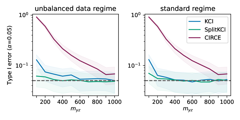
Figure 1: Task 1 with the significance level $\alpha\!=\!0.05$. Gray dashed line: $\alpha$. Left panel: unbalanced data regime ($n\!=\!m_{xz}\!=\!100$, growing $m_{yz}$). Right panel: standard data regime ($n\!=\!100$, growing $m_{xz}\!=\!m_{yz}$).

Task 2 (power comparison).

This task shows advantage of kernel-based methods for test power. We consider the following setup (with $\xi_{i}$ as in Task 1):

$$Z=\frac{\xi_{1}}{\|\xi_{1}\|_{2}}\,,\ Y=Z+\gamma\,\xi_{2}\,,\ X=Z+(\gamma\,\xi_{3})^{2}\,.$$

Type I error (Figure 2, top) of SplitKCI outperforms that of KCI in both settings, although it only reaches the desired level in the standard one with these sample sizes. GCM and RBPT2’, in contrast, have good control over Type I error.

The result is reversed for Type II error (Figure 2, bottom): GCM and RBPT2’ almost never reject the null, while kernel-based methods maintain high power (albeit better in the standard regime than unbalanced). This behavior is expected for GCM: the noise in $X$ and $Y$ is uncorrelated even under the alternative, making $X\!-\!\mathbb{E}\left[X\,|\,Z\right]$ and $Y\!-\!\mathbb{E}\left[Y\,|\,Z\right]$ uncorrelated too. Since kernel-based methods compute correlations for non-linear feature vectors $\phi_{x}(X)$ and $\phi_{y}(Y)$, they can detect such dependencies.

For KCI and SplitKCI, this result illustrates the trade-off between test power and training data size: as KCI has a larger estimation bias, it rejects more often due to this bias. For both measures, the error rate increases slightly with more training data, since the estimation bias becomes smaller. Type II error further decreases if we increase the dataset size (see Figure 9(d) in the appendix). Moreover, Type II error for RBPT2’ can be brought down to 0.2-0.4 (but higher than for (Split)KCI) for the Gaussian kernel for $g$ and selection of the best kernel for $h$; see Figures 10(b) and 10(d) in the appendix).

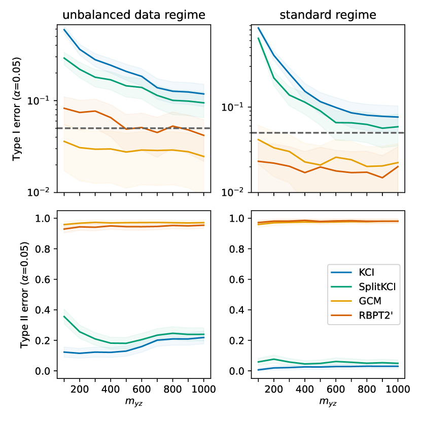
Figure 2: Task 2. $\alpha\!=\!0.05$. Left: unbalanced data regime ($n\!=\!m_{xz}=100$, growing $m_{yz}$). Right: standard data regime ($n\!=\!100$, growing $m_{xz}\!=\!m_{yz}$). Top: Type I error, gray dashed line: $\alpha$. Bottom: Type II error.

Task 3 (non-universal kernels).

Task 3 illustrates the importance of $Z$-kernel choice when the data are limited. We consider the following setting:

$$Z\!=\!\frac{f\left(g\left(\xi_{1}\right)\right)}{\|\xi_{1}\|_{2}}\,,\ Y\!=\!\frac{Z}{\|Z\|_{2}}\!+\!\gamma\,\xi_{2}\,,\ X\!=\!\frac{Z}{\|Z\|_{2}}\!+\!\gamma\,\xi_{3}\,,$$

$$g(z)=z+z\,\Theta((z)_{1})\,,\ f(z)=z-\frac{z}{2}\Theta(-(z)_{2})\,,$$

for the Heaviside step function $\Theta$ (of a single coordinate). If the kernel over $Z$ normalizes data points, it essentially solves Task 1. However, data normalization makes the kernel non-universal, and hence we do this only for $\mu_{X\,|\,Z}$.

This knowledge might not be available to us a priori – thus we test if selecting the best kernel through leave-one-out error (8) can find such patterns in $Z$. We run this task by choosing the $Z$-kernel for $\mu_{X\,|\,Z}$ by minimizing (8) over a set of kernels (Gaussian, polynomial, polynomial with normalization). For GCM, we also use this procedure for $\mu_{X\,|\,Z}$; for RBPT2’, we do it for $h(Z)$ while switching the kernel for $g(Y,Z)$ from linear to Gaussian to make the $g$ more expressive.

Figure 3: Task 3. Type I error for $\alpha\!=\!0.05$, gray dashed line. Left: unbalanced data regime ($n\!=\!m_{xz}\!=\!100$, growing $m_{yz}$). Right: standard data regime ($n\!=\!100$, growing $m_{xz}\!=\!m_{yz}$). Top: Gaussian kernel for $\mu_{X\,|\,Z}$ (GCM, (Split)KCI) and linear $g/$Gaussian $h$ (RBPT2’). Bottom: best of several kernels for $\mu_{X\,|\,Z}$ (GCM, (Split)KCI) and Gaussian $g/$best $h$ (RBPT2’).

In this task, GCM generally performs well and RBPT2’ does not (Figure 3 for $n\!=\!100$; for $n\!=\!200$ see Figures 11 and 12 in the Appendix). For GCM, this is due to the simple noise model as in Tasks 1/2. For RBPT2’, this is likely due to the estimation errors in the first regression $g(Y,Z)\!=\!\mu_{X\,|\,YZ}$. KCI and SplitKCI do not reach the desired Type I error in the unbalanced data regime, indicating a large estimation bias. With a flexible $Z$-kernel (Figure 3, bottom), both methods improve. In the unbalanced data regime, KCI still does not achieve the desired error rate, but SplitKCI does: both bias reduction and kernel flexibility of SplitKCI play a role.

Task 4 (high-dimensional $Z$).

This is a set of tasks taken from Polo et al. (2023), featuring a random quadratic dependence and a $d$-dimensional $Z$ with scalar $X$ and $Y$:

$$Z\sim\mathcal{N}(0,I_{d})\,,\quad Y=(Z^{\top}b)^{2}+\mathcal{N}(0,1)\,,$$

$$X=Z^{\top}a+\gamma(Z^{\top}b)^{2}+\mathcal{N}(0,1)+c\,Y\,,$$

$$\mathrm{H_{0}}:c=0\,,\ \mathrm{H_{1}}:c>0\,,$$

where for each random task we draw $a\!\sim\!\mathcal{N}(0,I_{d})\,,\ b\!\sim\!\mathcal{N}(0,I_{d})$; we also rescale the data as $X/\sqrt{d},Y/d,Z\sqrt{d}$ to normalize it. Large $\gamma$ makes Type I error control hard, due to marginal dependence between $X$ and $Y$. Large $c$ makes Type II error control easy, due to a more pronounced conditional dependency. We follow the task structure of Polo et al. (2023), testing for the hardest cases: $d\!=\!40;\mathrm{H_{0}:}\,\gamma\!=\!0.02,c\!=\!0;\mathrm{H_{1}:}\,\gamma\!=\!0,c\!=\!0.1$, with average results over 5 samples of $a,b$. In all cases, we use 200 test points.

Figure 4 shows results for the best kernel selection (Gaussian kernel performance was slightly worse for all methods, but especially GCM and RBPT2’; see Figure 13(a) in the appendix). For GCM and RBPT2’, the performance is poor and generally consistent with the results of Polo et al. (2023), who compare with methods that can sample from $P(Y\,|\,Z)$). While the kernel-based methods do not achieve the desired error rate, they vastly outperform the other two methods.

Figure 4: Task 4, Type I error (top) and Type II error (bottom) for $\alpha\!=\!0.05$ with $d\!=\!40$ and best kernel selection.

5.2 Real data

Following the setup of Polo et al. (2023), we test our methods on the car insurance dataset originally collected from four US states and multiple insurance companies by Angwin et al. (2017), with three variables: car insurance price $X$, minority neighborhood indicator $Y$ (defined as more that 66% non-white in California and Texas, and more that 50% in Missouri and Illinois), and driver’s risk $Z$ (with additional equalization of driver-related variables; see Angwin et al.).

We follow the data assessment experiment from Polo et al. (2023) to evaluate different methods under a simulated $\mathrm{H}_{0}$. Polo et al. (2023) divided the driver’s risk into 20 clusters, and shuffled the corresponding insurance price (per company and per state). The resulting data was evaluated for several tests, with average (over companies) rejection rate reported as Type I error. Following the same procedure, we find (see Figure 5) that both KCI and SplitKCI produce robust results at the desired $\alpha\!=\!0.05$ level. (CIRCE is slightly worse; see Section C.2.) While RBPT2 results in a smaller Type I error, this is undesirable since the statistic doesn’t follow the simulated distribution.

We also ran all tests on the full dataset (with 70/30% train/test split). As in Polo et al. (2023), RBPT and RBPT2 did not reject the null at $\alpha\!=\!0.05$ for California data, but did for the other states. All other methods, including the bias-corrected RBPT2’, rejected the null for all states. The results are summarized in Figure 13(b) of Section C.2.

Figure 5: Simulated null hypothesis for the car insurance data. RBPT(2): Polo et al. (2023); GCM: Shah and Peters (2020); KCI: Zhang et al. (2011); SplitKCI: ours.

6 Discussion

We have studied the performance of kernel-based measures of conditional independence in settings with limited data. While all studied methods are asymptotically equivalent, in practice they have very different Type I/II error performance. Our SplitKCI method reduces the bias in kernel-based measures, improving Type I error control. It also exhibits more flexibility to kernel choice, allowing for non-universal kernels (in some parts of the statistic) without sacrificing asymptotic power. In experiments, we showed that SplitKCI produces more stable Type-1 errors, at the cost of slightly increased Type-2 errors, and benefits greatly from auxiliary data. It also performs competitively with non-kernel-based measures on synthetic and real data. SplitKCI allows choosing the kernel over $Z$ for the $\mu_{X\,|\,Z}$ regression, which can further improve its performance for structured data; this is a topic of interest for future work. For instance, when $X$ is categorical, we can replace kernel ridge regression with logistic regression, or any classifier, with a linear kernel on top; this produces accurate predictions of $X$ that are not limited by simple hand-crafted kernels.

Conditional dependence tests are often used for sensitive domains in which the conclusions of a study can have significant societal impacts (e.g. Angwin et al., 2017). A further important topic for future work is therefore test interpretability, since conditional (in)dependence may be caused by unknown confounding variables.

Appendices

We present the proofs of the technical results in Appendix A. Details about other measures of conditional independence are presented in Appendix B. Appendix C contains experimental details, as well as additional experiments.

Appendix A Proofs

A.1 SplitKCI definition

See 2

Proof.

Using linearity of expectation, we have that

$$C_{\omega_{x}}\, =\mathbb{E}\left((\phi_{x}(X)-\omega_{x}(Z))\otimes\phi_{z}(Z)\otimes(\phi_{y}(Y)-\mu_{Y\,|\,Z}(Z))\right)$$

$$=\mathbb{E}\left(\phi_{x}(X)\otimes\phi_{z}(Z)\otimes(\phi_{y}(Y)-\mu_{Y\,|\,Z}(Z))\right)-\mathbb{E}\left(\omega_{x}(Z)\otimes\phi_{z}(Z)\otimes(\phi_{y}(Y)-\mu_{Y\,|\,Z}(Z))\right)\,.$$

The last term is zero:

$$\mathbb{E}\left(\omega_{x}(Z)\otimes\phi_{z}(Z)\otimes(\phi_{y}(Y)-\mu_{Y\,|\,Z}(Z))\right)=\mathbb{E}\left(\mathbb{E}\left[\omega_{x}(Z)\otimes\phi_{z}(Z)\otimes(\phi_{y}(Y)-\mu_{Y\,|\,Z}(Z))\,|\,Z\right]\right)=0\,.$$

Therefore, $\left<C_{\omega_{x}^{(1)}},\,C_{\omega_{x}^{(2)}}\right>_{\mathrm{HS}}=\|C_{\mathrm{CIRCE}}\|_{\mathrm{HS}}^{2}$ (and, using the same calculation, it equals to $\|C_{\mathrm{KCI}}\|_{\mathrm{HS}}^{2}$).

Since the empirical estimator in Equation 5 is a standard mean estimator of a product of kernel matrices for two independent variables $(X,Y,Z)$ and $(X^{\prime},Y^{\prime},Z^{\prime})$, we only need to modify $K^{c}_{X}$ to follow

$$(K^{c}_{X})_{ij}=\left<\phi_{x}(x_{i})-\omega_{x}^{(1)}(z_{i}),\,\phi_{x}(x_{j})-\omega_{x}^{(2)}(z_{j})\right>\,.\qed$$

A.2 Bias

See 3

Proof.

We will consider the HSIC-style estimator for both KCI (with train data $\mathcal{D}_{\mathrm{train}}^{m_{xz}}$ and $\mathcal{D}_{\mathrm{train}}^{m_{yz}}$) and SplitKCI (with train data over $(xz)$ split into $\mathcal{D}_{\mathrm{train}}^{m_{xz}/2}$ and $\mathcal{D}_{\mathrm{train}}^{m_{xz}/2}$) simultaneously in the initial derivation with train sets (over $(xz)$) $\mathcal{D}_{\mathrm{train}}^{m_{xz}^{1}}$ and $\mathcal{D}_{\mathrm{train}}^{m_{xz}^{2}}$, assuming that $\widehat{\mu}_{X\,|\,Z}^{(1)}=\widehat{\mu}_{X\,|\,Z}^{(2)}$ for KCI. Denoting

$$(\widehat{K}_{YZ\,|\,Z})_{ij}\, =(K_{Z}\odot\widehat{K}^{c}_{Y})_{ij}=k_{z}(z_{i},z_{j})\,\left<\phi_{y}(y_{i})-\widehat{\mu}_{Y\,|\,Z}(z_{i}),\,\phi_{y}(y_{j})-\widehat{\mu}_{Y\,|\,Z}(z_{j})\right>\,,$$

$$(\widehat{K}^{c}_{X})_{ij}\, =\frac{1}{2}(\widehat{K}^{12}_{X})_{ij}+\frac{1}{2}(\widehat{K}^{21}_{X})_{ij}\,,\quad(\widehat{K}^{12}_{X})_{ij}=\left<\phi_{x}(x_{i})-\widehat{\mu}_{X\,|\,Z}^{(1)}(z_{i}),\,\phi_{x}(x_{j})-\widehat{\mu}_{X\,|\,Z}^{(2)}(z_{j})\right>\,,$$

we can compute the expectation (over $\mathcal{D}_{\mathrm{train}}^{m_{xz}^{1}},\mathcal{D}_{\mathrm{train}}^{m_{xz}^{2}},\mathcal{D}_{\mathrm{train}}^{m_{yz}}$ and points $i,j$). Additionally decomposing

$$\widehat{\mu}_{X\,|\,Z}^{(1)}\, =\mu_{X\,|\,Z}+(\mu_{X\,|\,Z}^{\lambda}-\mu_{X\,|\,Z})+(\mu_{X\,|\,Z}^{\lambda}-\widehat{\mu}_{X\,|\,Z}^{(1)})=\mu_{X\,|\,Z}+\delta\mu_{X\,|\,Z}^{\lambda}+\delta\widehat{\mu}_{X\,|\,Z}^{(1)\lambda}\,,$$

$$\widehat{\mu}_{Y\,|\,Z}\, =\mu_{Y\,|\,Z}+(\mu_{Y\,|\,Z}-\widehat{\mu}_{Y\,|\,Z})=\mu_{Y\,|\,Z}+\delta\widehat{\mu}_{Y\,|\,Z}=\mu_{Y\,|\,Z}+\delta\mu_{Y\,|\,Z}^{\lambda}+\delta\widehat{\mu}_{Y\,|\,Z}^{\lambda}\,,$$

where we decompose the empirical estimate of the mean into the true one, the distance between the true one and the expected estimate given the ridge parameters, and finally between the ridge mean and its estimate (so that the last term is zero-mean).

Under the null, we can immediately remove the terms with the true centered variables $\phi_{x}(x_{i})-\mu_{X\,|\,Z}^{(1)}(z_{i})$:

$$\mathbb{E}\,(\widehat{K}^{12}_{X})_{ij}\,(\widehat{K}_{YZ\,|\,Z})_{ij}$$

$$=\mathbb{E}\,\left<\phi_{x}(x_{i})-\widehat{\mu}_{X\,|\,Z}^{(1)}(z_{i}),\,\phi_{x}(x_{j})-\widehat{\mu}_{X\,|\,Z}^{(2)}(z_{j})\right>(\widehat{K}_{YZ\,|\,Z})_{ij}$$

$$=_{\mathrm{H}_{0}}\mathbb{E}\,\left<\delta\mu_{X\,|\,Z}^{\lambda}(z_{i})+\delta\widehat{\mu}_{X\,|\,Z}^{(1)\lambda}(z_{i}),\,\delta\mu_{X\,|\,Z}^{\lambda}(z_{j})+\delta\widehat{\mu}_{X\,|\,Z}^{(2)\lambda}(z_{j})\right>(\widehat{K}_{YZ\,|\,Z})_{ij}$$

$$=\mathbb{E}\,\left[\left<\delta\mu_{X\,|\,Z}^{\lambda}(z_{i}),\,\delta\mu_{X\,|\,Z}^{\lambda}(z_{j})\right>+\left<\delta\widehat{\mu}_{X\,|\,Z}^{(1)\lambda}(z_{i}),\,\delta\widehat{\mu}_{X\,|\,Z}^{(2)\lambda}(z_{j})\right>\right](\widehat{K}_{YZ\,|\,Z})_{ij}$$

$$=_{\mathrm{H}_{0}}\mathbb{E}\,\left[\left<\delta\mu_{X\,|\,Z}^{\lambda}(z_{i}),\,\delta\mu_{X\,|\,Z}^{\lambda}(z_{j})\right>+\left<\delta\widehat{\mu}_{X\,|\,Z}^{(1)\lambda}(z_{i}),\,\delta\widehat{\mu}_{X\,|\,Z}^{(2)\lambda}(z_{j})\right>\right]k_{z}(z_{i},z_{j})\left<\delta\widehat{\mu}_{Y\,|\,Z}(z_{i}),\,\delta\widehat{\mu}_{Y\,|\,Z}(z_{j})\right>\,,$$

where in the third line we took the expectation over $\mathcal{D}_{\mathrm{train}}^{m_{xz}^{1}},\mathcal{D}_{\mathrm{train}}^{m_{xz}^{2}}$ using the facts that $\mathbb{E}\,\delta\widehat{\mu}_{X\,|\,Z}^{1/2\lambda}=0$ and that all data splits (apart from $\mathcal{D}_{\mathrm{train}}^{m_{xz}^{1}},\mathcal{D}_{\mathrm{train}}^{m_{xz}^{2}}$) are independent, and in the last line, we used centering with $\phi_{y}(y_{i})-\mu_{Y\,|\,Z}(z_{i})$ under the null.

Now, for SplitKCI we can take the expectation w.r.t. the train data, removing the zero-mean $\left<\delta\widehat{\mu}_{X\,|\,Z}^{(1)\lambda}(z_{i}),\,\delta\widehat{\mu}_{X\,|\,Z}^{(2)\lambda}(z_{j})\right>$ term, and denote the bias as $b_{\mathrm{SplitKCI}}$:

$$b_{\mathrm{SplitKCI}}=\mathbb{E}\,(\widehat{K}^{12}_{X})_{ij}\,(\widehat{K}_{YZ\,|\,Z})_{ij}=_{\mathrm{H}_{0}}\mathbb{E}\,\left<\delta\mu_{X\,|\,Z}^{\lambda}(z_{i}),\,\delta\mu_{X\,|\,Z}^{\lambda}(z_{j})\right>k_{z}(z_{i},z_{j})\left<\delta\widehat{\mu}_{Y\,|\,Z}(z_{i}),\,\delta\widehat{\mu}_{Y\,|\,Z}(z_{j})\right>\,.$$ (9)

For KCI, since the estimators are the same, the bias $b_{\mathrm{KCI}}$ term becomes

$$b_{\mathrm{KCI}}=_{\mathrm{H}_{0}}\mathbb{E}\,\left[\left<\delta\mu_{X\,|\,Z}^{\lambda}(z_{i}),\,\delta\mu_{X\,|\,Z}^{\lambda}(z_{j})\right>+\left<\delta\widehat{\mu}_{X\,|\,Z}^{\lambda}(z_{i}),\,\delta\widehat{\mu}_{X\,|\,Z}^{\lambda}(z_{j})\right>\right]k_{z}(z_{i},z_{j})\left<\delta\widehat{\mu}_{Y\,|\,Z}(z_{i}),\,\delta\widehat{\mu}_{Y\,|\,Z}(z_{j})\right>\,.$$ (10)

Now, for datasets of equal size, the KCI bias is clearly larger than the SplitKCI one. However, in practice we’d use twice as many points for KCI, so the exact scaling of the terms is important.

To bound the individual terms, we first note that since we assumed the CME is well-specified, we can use the reproducing property $\left<\mu_{X\,|\,Z}(z),\,h\right>_{\mathcal{H}_{x}}=\left<\mu_{X\,|\,Z},\,\phi_{z}(z)\otimes h\right>_{\mathrm{HS}}$ to show that $\|\mu_{X\,|\,Z}(z)\|\leq\|\mu_{X\,|\,Z}\|k_{z}(z,z)^{1/2}$, and hence by Cauchy-Schwarz

$$\left<\delta\mu_{X\,|\,Z}^{\lambda}(z_{i}),\,\delta\mu_{X\,|\,Z}^{\lambda}(z_{j})\right>\leq\|\delta\mu_{X\,|\,Z}^{\lambda}\|^{2}\,k_{z}(z_{i},z_{i})^{1/2}k_{z}(z_{j},z_{j})^{1/2}\leq\|\delta\mu_{X\,|\,Z}^{\lambda}\|^{2}\,,$$

assuming the kernels are bounded by 1. We can extend this to all products, again using independence of data splits (so $\|\delta\widehat{\mu}_{X\,|\,Z}^{\lambda}\|^{2}$ and $\|\delta\widehat{\mu}_{Y\,|\,Z}\|^{2}$ are independent) and the fact that $\|\delta\mu_{X\,|\,Z}^{\lambda}\|^{2}$ is deterministic,

$$b_{\mathrm{SplitKCI}}\, \leq_{\mathrm{H}_{0}}\mathbb{E}\,\|\delta\mu_{X\,|\,Z}^{\lambda}\|^{2}\,\|\delta\widehat{\mu}_{Y\,|\,Z}\|^{2}=\|\delta\mu_{X\,|\,Z}^{\lambda}\|^{2}\,\mathbb{E}\,\|\delta\widehat{\mu}_{Y\,|\,Z}\|^{2}\,,$$

$$b_{\mathrm{KCI}}\, \leq_{\mathrm{H}_{0}}\mathbb{E}\,\left[\|\delta\mu_{X\,|\,Z}^{\lambda}\|^{2}+\|\delta\widehat{\mu}_{X\,|\,Z}^{\lambda}\|^{2}\right]\,\|\delta\widehat{\mu}_{Y\,|\,Z}\|^{2}=\left[\|\delta\mu_{X\,|\,Z}^{\lambda}\|^{2}+\mathbb{E}\,\|\delta\widehat{\mu}_{X\,|\,Z}^{\lambda}\|^{2}\right]\,\mathbb{E}\,\|\delta\widehat{\mu}_{Y\,|\,Z}\|^{2}\,,$$

Now, with our assumptions about CME convergence, we can directly use Theorem 2 of Li et al. (2022b), (with $\gamma=1$, $\alpha=1$ and $\beta\in(1,2]$ to match the required HS norm and the well-specified case): $\|\delta\widehat{\mu}_{Y\,|\,Z}\|^{2}\leq\tau^{2}\,K_{yz}(m_{yz})^{-\frac{\beta-1}{\beta+p}}$ for large enough $m_{yz}$ and a positive constant $K_{yz}$ with probability at least $1-4e^{-\tau}$ for $\tau\geq 1$. Hence, we can write down the expectation as an integral and split it at $t^{*}=K_{yz}(m_{yz})^{-\frac{\beta-1}{\beta+p}}$ corresponding to $\tau=1$:

$$\mathbb{E}\,\|\delta\widehat{\mu}_{Y\,|\,Z}\|^{2}\, =\int_{0}^{\infty}\mathbb{P}\left(\|\delta\widehat{\mu}_{Y\,|\,Z}\|^{2}\geq t\right)dt=\int_{0}^{t^{*}}\mathbb{P}\left(\|\delta\widehat{\mu}_{Y\,|\,Z}\|^{2}\geq t\right)dt+\int_{t^{*}}^{\infty}\mathbb{P}\left(\|\delta\widehat{\mu}_{Y\,|\,Z}\|^{2}\geq t\right)dt$$

$$\leq\int_{0}^{t^{*}}1dt+\int_{0}^{\infty}4\,\exp\left(-\sqrt{t\,\frac{1}{K_{yz}}m_{yz}^{\frac{\beta-1}{\beta+p}}}\right)dt=9\,K_{yz}m_{yz}^{-\frac{\beta-1}{\beta+p}}\,.$$

By the exact same argument, and using the bias-variance decomposition of the bound (Eq. 12 of Li et al. (2022b) and then the proof in Appendix A.3),

$$\mathbb{E}\,\|\delta\widehat{\mu}_{X\,|\,Z}^{\lambda}\|^{2}\leq\|\delta\mu_{X\,|\,Z}^{\lambda}\|^{2}+9\,K_{xz}m_{xz}^{-\frac{\beta-1}{\beta+p}}.$$ (11)

Finally, by Lemma 1 of A.1 Li et al. (2022b), we have a (deterministic) bound (note a different HS norm defined by the $\beta$ interpolation space; the standard norm corresponds to $\beta=1$; see more details in Li et al. (2022b)):

$$\|\delta\mu_{X\,|\,Z}^{\lambda}\|^{2}\leq\|\mu_{X\,|\,Z}\|^{2}_{\beta}\lambda^{\beta-1}=\|\mu_{X\,|\,Z}\|^{2}_{\beta}\,m_{xz}^{-\frac{\beta-1}{\beta+p}}$$

where we used the optimal learning rate $\lambda=m_{xz}^{-\frac{1}{\beta+p}}$.

It remains to compare the bias in KCI for the full train set and SplitKCI for halved sets. The constant $K_{xz}$ in Equation 11 is a sum of positive terms, with one of them being $576\,A^{2}\,\|\mu_{X\,|\,Z}\|^{2}_{\beta}$, where for the well-specified case of $\alpha=1$ and $A^{2}$ can be defined as the supremum norm of $k_{y}$ (see Fischer and Steinwart (2020), Theorem 9). Since we assumed that $k_{y}$ is bounded by one, the KCI bound (Equation 11) becomes

$$\mathbb{E}\,\|\delta\widehat{\mu}_{X\,|\,Z}^{\lambda}\|^{2}\leq\|\mu_{X\,|\,Z}\|^{2}_{\beta}\,m_{xz}^{-\frac{\beta-1}{\beta+p}}+9\cdot 576\,\|\mu_{X\,|\,Z}\|^{2}_{\beta}\,m_{xz}^{-\frac{\beta-1}{\beta+p}}+K_{1}m_{xz}^{-\frac{\beta-1}{\beta+p}}=(1+K_{1})\,\|\mu_{X\,|\,Z}\|^{2}_{\beta}\,m_{xz}^{-\frac{\beta-1}{\beta+p}}+K_{2}m_{xz}^{-\frac{\beta-1}{\beta+p}}\,,$$

for $K_{1}=5184$ and $K_{2}>0$.

For SplitKCI with half the data, we get

$$\|\delta\mu_{X\,|\,Z}^{\lambda}\|^{2}\leq\|\mu_{X\,|\,Z}\|^{2}_{\beta}\,\left(\frac{m_{xz}}{2}\right)^{-\frac{\beta-1}{\beta+p}}\leq 2\|\mu_{X\,|\,Z}\|^{2}_{\beta}\,m_{xz}^{-\frac{\beta-1}{\beta+p}}\,.$$

Combining the bounds and denoting $K_{3}=K_{yz}$ for simplicity finishes the proof. ∎

A.3 Wild bootstrap

See 4

Before beginning the proof, we note that in practice we use the unbiased estimator in Equation 17, which corresponds to a U-statistic. The only difference between the U- and V-statistics of Equations 5 and 17 is essentially removal of the terms $i=j$ in the sum (the scaling is also adapted accordingly). See Kim and Schrab (2023, Lemma 22) for an expression of the difference between U- and V-statistics for the closely-related HSIC case.

Proof.

We start by setting up the notations. Let

$$(K^{c}_{X})_{ij}\! =\!\left<\phi_{x}(X_{i})\!-\!\mu_{X\,|\,Z}(Z_{i}),\,\phi_{x}(X_{j})\!-\!\mu_{X\,|\,Z}(Z_{j})\right>, (\widehat{K}^{c}_{X})_{ij}\! =\!\left<\phi_{x}(X_{i})\!-\!\widehat{\mu}_{X\,|\,Z}(Z_{i}),\,\phi_{x}(X_{j})\!-\!\widehat{\mu}_{X\,|\,Z}(Z_{j})\right>,$$

and similarly for $Y$ instead of $X$. The $V$-statistics and wild bootstrap KCI estimates using the true and estimated conditional mean embeddings are given as

$$V=\frac{1}{n^{2}}\sum_{1\leq i,j\leq n}(K^{c}_{X})_{ij}(K_{Z})_{ij}(K^{c}_{Y})_{ij}, B=\frac{1}{n^{2}}\sum_{1\leq i,j\leq n}q_{i}q_{j}\,(K^{c}_{X})_{ij}(K_{Z})_{ij}(K^{c}_{Y})_{ij},$$

$$\widehat{V}=\frac{1}{n^{2}}\sum_{1\leq i,j\leq n}(\widehat{K}^{c}_{X})_{ij}(K_{Z})_{ij}(\widehat{K}^{c}_{Y})_{ij}, \widehat{B}=\frac{1}{n^{2}}\sum_{1\leq i,j\leq n}q_{i}q_{j}\,(\widehat{K}^{c}_{X})_{ij}(K_{Z})_{ij}(\widehat{K}^{c}_{Y})_{ij}.$$

We focus on the KCI case, as the proof for CIRCE follows very similarly (the only difference is that the centered kernel matrix $K^{c}_{X}$ is replaced with its non-centered version $K_{X}$). The reasoning also applies to SplitKCI. We emphasize that the conditional mean embeddings $\widehat{\mu}_{X\,|\,Z}$, $\widehat{\mu}_{Y\,|\,Z}$ do not admit close forms and have to be estimated using the CME estimator (see Equation 6) on held-out data.

We prove below that

1. under the null $n(\widehat{V}-V)\to 0$ and $n(\widehat{B}-B)\to 0$ in probability,

2. under the alternative $(\widehat{V}-V)\to 0$ and $(\widehat{B}-B)\to 0$ in probability.

Before proving (i) and (ii), we first show that they imply the desired results. Chwialkowski et al. (2014) study the wild bootstrap generally and handle the MMD and HSIC as special cases. Similarly to their HSIC setting, a symmetrisation trick can be performed for KCI and CIRCE. We rely on their general results which assume a weaker $\tau$-mixing assumption which is trivially satisfied the i.i.d. setting we consider, we point that similar results can be found in Wu (1986); Shao (2010); Leucht and Neumann (2013).

Under the null, we have

$$n(\widehat{V}-\widehat{B})=n(\widehat{V}-V)+n(V-B)+n(B-\widehat{B})$$

where by (i) $n(\widehat{V}-V)\to 0$ and $n(B-\widehat{B})\to 0$ in probability. Chwialkowski et al. (2014, Theorem 1) also guarantees that $n(V-B)\to 0$ weakly. We conclude that $n(\widehat{V}-\widehat{B})\to 0$ weakly, that is, $n\widehat{B}$ and $n\widehat{V}$ converge weakly to the same distribution under the null.

Under the alternative, by (ii) we have $(\widehat{V}-V)\to 0$ and $(B-\widehat{B})\to 0$ in probability. Moreover, Chwialkowski et al. (2014, Theorems 3 and 2) guarantees that $B\to 0$ in mean squared and that $V\to c$ in mean squared for some $c>0$, respectively. We conclude that

$$\widehat{B}=(\widehat{B}-B)+B\to 0\qquad\textrm{ and }\qquad\widehat{V}=(\widehat{V}-V)+V\to c$$

in probability. ∎

Proof of (i) and (ii).

This proof adapts the reasoning of Chwialkowski et al. (2014, Lemma 3) for HSIC to hold for KCI. This is particularly challenging because while the mean embedding admits a closed form, the conditional mean embedding does not and has weaker convergence properties (Li et al., 2022b, 2023). We provide results in probability rather than in expectation (one can use Markov’s inequality to turn an expected bound into one holding with high probability). Let us define

$$T_{n} =\frac{1}{n}\sum_{i=1}^{n}Q_{i}(\phi_{x}(X_{i})-\mu_{X\,|\,Z}(Z_{i}))\otimes\phi_{z}(Z_{i})\otimes(\phi_{y}(Y_{i})-\mu_{Y\,|\,Z}(Z_{i})),$$

$$\widehat{T}_{n} =\frac{1}{n}\sum_{i=1}^{n}Q_{i}(\phi_{x}(X_{i})-\widehat{\mu}_{X\,|\,Z}(Z_{i}))\otimes\phi_{z}(Z_{i})\otimes(\phi_{y}(Y_{i})-\widehat{\mu}_{Y\,|\,Z}(Z_{i})),$$

where, either $Q_{i}=q_{i}$, $i=1,\dots,n$ Rademacher variable in which case

$$\|T_{n}\|^{2}=\frac{1}{n^{2}}\sum_{1\leq i,j\leq n}q_{i}q_{j}\,(K^{c}_{X})_{ij}(K_{Z})_{ij}(K^{c}_{Y})_{ij}=B\qquad\textrm{ and }\qquad\|\widehat{T}_{n}\|^{2}=\widehat{B},$$

or $Q_{i}=1$, $i=1,\dots,n$ in which case $\|T_{n}\|^{2}=V$ and $\|\widehat{T}_{n}\|^{2}=\widehat{V}$. So it suffices to prove

1. under the null $n(\|\widehat{T}_{n}\|^{2}-\|T_{n}\|^{2})\to 0$ in probability,

2. under the alternative $(\|\widehat{T}_{n}\|^{2}-\|T_{n}\|^{2})\to 0$ in probability.

We can obtain these results provided that

1. $\|\sqrt{n}(\widehat{T}_{n}-T_{n})\|\to 0$ in probability,

which we prove below. For now, assume (iii) holds.

Under the null, we then have

$$n\,\Big{|}\|\widehat{T}_{n}\|^{2}-\|T_{n}\|^{2}\Big{|} \leq n\,\Big{|}\|\widehat{T}_{n}\|-\|T_{n}\|\Big{|}\,\Big{|}\|\widehat{T}_{n}\|+\|T_{n}\|\Big{|}$$

$$\leq\sqrt{n}\,\|(\widehat{T}_{n}-T_{n})\|\Big{(}\sqrt{n}\,\|\widehat{T}_{n}\|+\sqrt{n}\,\|T_{n}\|\Big{)}$$

$$\to 0$$

in probability, provided that $\sqrt{n}\|T_{n}\|<\infty$, which is guaranteed by Chwialkowski et al. (2014, Lemma 4) under the null ($\Delta=0$ in Lemma 4 notation since we’re working with the i.i.d. case), and that $\sqrt{n}\,\|\widehat{T}_{n}\|<\infty$, both with arbitrarily high probability. The latter holds since

$$\sqrt{n}\,\|\widehat{T}_{n}\|\leq\sqrt{n}\,\|\widehat{T}_{n}-T_{n}\|+\sqrt{n}\,\|T_{n}\|$$

where the first term tends to zero due to the assumed $m_{xz},m_{yz}$ scaling and the second is bounded, with arbitrarily high probability. This proves (i).

Under the alternative, we obtain

$$\Big{|}\|\widehat{T}_{n}\|^{2}-\|T_{n}\|^{2}\Big{|} \leq\Big{|}\|\widehat{T}_{n}\|-\|T_{n}\|\Big{|}\,\Big{|}\|\widehat{T}_{n}\|+\|T_{n}\|\Big{|}$$

$$\leq\|(\widehat{T}_{n}-T_{n})\|\Big{(}\|\widehat{T}_{n}\|+\|T_{n}\|\Big{)}$$

$$\to 0$$

in probability, as $\|T_{n}\|<\infty$ by bounding the kernels and the $Q_{i}$’s by 1, and

$$\|\widehat{T}_{n}\|\leq\sqrt{n}\,\|\widehat{T}_{n}-T_{n}\|+\|T_{n}\|$$

with again the first term tending to zero and the second one being bounded, with arbitrarily high probability. This proves (ii). ∎

Proof of (iii).

Li et al. (2023, Theorem 2.2.a), with $\gamma=1$, $\beta\in(1,2]$, $\alpha=1$ (see 1), provides a rate of convergence in RKHS norm for the CME estimator when the true conditional mean embedding lies within a $\beta$-smooth subset of the RKHS ($\beta=1$ would correspond to the full RKHS). There exists a constant $C>0$ independent of $m_{xz}$ and $\tau$ such that

$$\|\widehat{\mu}_{X\,|\,Z}-\mu_{X\,|\,Z}\|\leq C\tau m_{xz}^{-\frac{\beta-1}{2(\beta+p)}}\qquad\textrm{with probability at least }1-5e^{-\tau}$$

for $m_{xz}$ sufficiently large and for all $\tau>\ln(5)$, where $p\in(0,1]$ induces a smoothness condition on the kernel used (its eigenvalues $\mu_{i}$ must decay as $i^{-1/p}$). As justified below, we will be interested in the scaled rate

$$\|\sqrt{n}(\widehat{\mu}_{X\,|\,Z}-\mu_{X\,|\,Z})\|\leq C\tau n^{\frac{1}{2}}m_{xz}^{-\frac{\beta-1}{2(\beta+p)}}.$$

Now, assuming that $m_{xz}=\omega\Big{(}n^{\frac{\beta+p}{\beta-1}}\Big{)}$ (i.e. $m_{xz}$ dominates $n^{\frac{\beta+p}{\beta-1}}$ asymptotically), then we obtain

$$\|\sqrt{n}(\widehat{\mu}_{X\,|\,Z}-\mu_{X\,|\,Z})\|\to 0$$ (12)

in probability as $n$ tends to infinity. Note that this trivially implies that

$$\|\widehat{\mu}_{X\,|\,Z}\|\leq\|\sqrt{n}(\widehat{\mu}_{X\,|\,Z}-\mu_{X\,|\,Z})\|+\|\mu_{X\,|\,Z}\|<\infty$$ (13)

for all $n\in\mathbb{N}$. The results in Equations (12 and 13 also hold using $Y$ instead of $X$.

We are now ready to show that $\|\sqrt{n}(\widehat{T}_{n}-T_{n})\|\to 0$ in probability. Note that

$$\sqrt{n}(\widehat{T}_{n}-T_{n}) =\frac{1}{\sqrt{n}}\sum_{i=1}^{n}Q_{i}\Bigg{(}(\phi_{x}(X_{i})-\widehat{\mu}_{X\,|\,Z}(Z_{i}))\otimes\phi_{z}(Z_{i})\otimes(\phi_{y}(Y_{i})-\widehat{\mu}_{Y\,|\,Z}(Z_{i}))$$

$$\hskip 68.28644pt-(\phi_{x}(X_{i})-\mu_{X\,|\,Z}(Z_{i}))\otimes\phi_{z}(Z_{i})\otimes(\phi_{y}(Y_{i})-\mu_{Y\,|\,Z}(Z_{i}))\Bigg{)}$$

$$=\frac{1}{\sqrt{n}}\sum_{i=1}^{n}Q_{i}\,\phi_{x}(X_{i})\otimes\phi_{z}(Z_{i})\otimes\Big{(}\mu_{Y\,|\,Z}(Z_{i})-\widehat{\mu}_{Y\,|\,Z}(Z_{i})\Big{)}$$ (14)

$$\hskip 14.22636pt+\frac{1}{\sqrt{n}}\sum_{i=1}^{n}Q_{i}\,\Big{(}\mu_{X\,|\,Z}(Z_{i})-\widehat{\mu}_{X\,|\,Z}(Z_{i})\Big{)}\otimes\phi_{z}(Z_{i})\otimes\phi_{y}(Y_{i})$$ (15)

$$\hskip 14.22636pt+\frac{1}{\sqrt{n}}\sum_{i=1}^{n}Q_{i}\,\Big{(}\widehat{\mu}_{X\,|\,Z}(Z_{i})\otimes\phi_{z}(Z_{i})\otimes\widehat{\mu}_{Y\,|\,Z}(Z_{i})-\mu_{X\,|\,Z}(Z_{i})\otimes\phi_{z}(Z_{i})\otimes\mu_{Y\,|\,Z}(Z_{i})\Big{)}.$$ (16)

The terms (14) and (15) can be handled in a similar fashion, the term (16) needs to be tackle separately. Note that in the CIRCE case we would have only the first term (14).

The term (14) is

$$\left\|\frac{1}{\sqrt{n}}\sum_{i=1}^{n}Q_{i}\,\phi_{x}(X_{i})\otimes\phi_{z}(Z_{i})\otimes\Big{(}\mu_{Y\,|\,Z}(Z_{i})-\widehat{\mu}_{Y\,|\,Z}(Z_{i})\Big{)}\right\|$$

$$\leq\ \frac{1}{n}\sum_{i=1}^{n}|Q_{i}|\left\|\,\phi_{x}(X_{i})\otimes\phi_{z}(Z_{i})\otimes\sqrt{n}\Big{(}\mu_{Y\,|\,Z}(Z_{i})-\widehat{\mu}_{Y\,|\,Z}(Z_{i})\Big{)}\right\|$$

$$=\ \frac{1}{n}\sum_{i=1}^{n}(k_{x}(X_{i},X_{i})k_{z}(Z_{i},Z_{i}))^{1/2}\left\|\sqrt{n}\Big{(}\mu_{Y\,|\,Z}(Z_{i})-\widehat{\mu}_{Y\,|\,Z}(Z_{i})\Big{)}\right\|$$

$$\leq\ \frac{1}{n}\sum_{i=1}^{n}k_{x}(X_{i},X_{i})^{1/2}k_{z}(Z_{i},Z_{i})\left\|\sqrt{n}\Big{(}\mu_{Y\,|\,Z}-\widehat{\mu}_{Y\,|\,Z}\Big{)}\right\|_{\mathrm{HS}}$$

$$\leq\ \left\|\sqrt{n}\Big{(}\mu_{Y\,|\,Z}-\widehat{\mu}_{Y\,|\,Z}\Big{)}\right\|$$

$$\to\ 0$$

in probability by Equation (12), where we the triangle inequality (2nd line), product space definition (3rd line), $\|\mu_{X\,|\,Z}(z)\|\leq\|\mu_{X\,|\,Z}\|k_{z}(z,z)^{1/2}$ (4th line) and the facts that $k_{x}$, $k_{z}$ and $Q_{i}$ are all bounded by 1.

Similarly, the second term (15) converges to 0 in probability.

For the third term (16), we have

$$\left\|\frac{1}{\sqrt{n}}\sum_{i=1}^{n}Q_{i}\,\Big{(}\widehat{\mu}_{X\,|\,Z}(Z_{i})\otimes\phi_{z}(Z_{i})\otimes\widehat{\mu}_{Y\,|\,Z}(Z_{i})-\mu_{X\,|\,Z}(Z_{i})\otimes\phi_{z}(Z_{i})\otimes\mu_{Y\,|\,Z}(Z_{i})\Big{)}\right\|$$

$$\leq\ \frac{1}{n}\sum_{i=1}^{n}|Q_{i}|\left\|\sqrt{n}\,\Big{(}\widehat{\mu}_{X\,|\,Z}(Z_{i})\otimes\phi_{z}(Z_{i})\otimes\widehat{\mu}_{Y\,|\,Z}(Z_{i})-\mu_{X\,|\,Z}(Z_{i})\otimes\phi_{z}(Z_{i})\otimes\mu_{Y\,|\,Z}(Z_{i})\Big{)}\right\|$$

$$=\ \frac{1}{n}\sum_{i=1}^{n}\sqrt{k_{z}(Z_{i},Z_{i})}\left\|\sqrt{n}\,\left(\widehat{\mu}_{X\,|\,Z}(Z_{i})\otimes\left(\widehat{\mu}_{Y\,|\,Z}(Z_{i})\pm\mu_{Y\,|\,Z}(Z_{i})\right)-\mu_{X\,|\,Z}(Z_{i})\otimes\mu_{Y\,|\,Z}(Z_{i})\right)\right\|$$

$$\leq\ \frac{1}{n}\sum_{i=1}^{n}\sqrt{k_{z}(Z_{i},Z_{i})}\left(\left\|\sqrt{n}\,\widehat{\mu}_{X\,|\,Z}(Z_{i})\otimes\left(\widehat{\mu}_{Y\,|\,Z}(Z_{i})-\mu_{Y\,|\,Z}(Z_{i})\right)\right\|+\left\|\sqrt{n}\,(\widehat{\mu}_{X\,|\,Z}(Z_{i})-\mu_{X\,|\,Z}(Z_{i}))\otimes\mu_{Y\,|\,Z}(Z_{i})\right\|\right)$$

$$=\ \frac{1}{n}\sum_{i=1}^{n}\sqrt{k_{z}(Z_{i},Z_{i})}\left(\left\|\widehat{\mu}_{X\,|\,Z}(Z_{i})\right\|\left\|\sqrt{n}\,\left(\widehat{\mu}_{Y\,|\,Z}(Z_{i})-\mu_{Y\,|\,Z}(Z_{i})\right)\right\|+\left\|\mu_{Y\,|\,Z}(Z_{i})\right\|\left\|\sqrt{n}\,(\widehat{\mu}_{X\,|\,Z}(Z_{i})-\mu_{X\,|\,Z}(Z_{i}))\right\|\right)$$

$$\leq\ \frac{1}{n}\sum_{i=1}^{n}\left(k_{z}(Z_{i},Z_{i})\right)^{3/2}\left(\left\|\widehat{\mu}_{X\,|\,Z}\right\|\left\|\sqrt{n}\,\left(\widehat{\mu}_{Y\,|\,Z}-\mu_{Y\,|\,Z}\right)\right\|+\left\|\mu_{Y\,|\,Z}\right\|\left\|\sqrt{n}\,(\widehat{\mu}_{X\,|\,Z}-\mu_{X\,|\,Z}\right\|\right)$$

$$\leq\ \Big{\|}\widehat{\mu}_{X\,|\,Z}\Big{\|}\Big{\|}\sqrt{n}\,(\widehat{\mu}_{Y\,|\,Z}-\mu_{Y\,|\,Z})\Big{\|}+\Big{\|}\mu_{Y\,|\,Z}\Big{\|}\Big{\|}\sqrt{n}\,(\widehat{\mu}_{X\,|\,Z}-\mu_{X\,|\,Z})\Big{\|}$$

$$\to\ 0$$

in probability by Equation (12), using the triangle inequality (second line), product spaces definition (third line), again triangle inequality (4th) and product spaces definition (5th) and then $\|\mu_{X\,|\,Z}(z)\|\leq\|\mu_{X\,|\,Z}\|k_{z}(z,z)^{1/2}$ and the fact that $k_{z}(z,z)$ and $Q_{i}$ are bounded by 1, with the final result holding since $\big{\|}\widehat{\mu}_{X\,|\,Z}\big{\|}<\infty$ by Equation (13).

We deduct that $\|\sqrt{n}(\widehat{T}_{n}-T_{n})\|\to 0$ in probability, which shows (iii).

This concludes the proof of Theorem 4.

∎

Appendix B Other measures of conditional independence

B.1 KCI

Notes on the original implementation

First, we note that the set $E_{1}^{\prime}=\{g\in L_{X}^{2}:\mathbb{E}\left[g(X)\,|\,Z\right]=0\}$ used in the original KCI formulation (Zhang et al., 2011) is not present in Theorem 1 of Daudin (1980). The theorem is proven for $E_{1}=\{g\in L_{XZ}^{2}:\mathbb{E}\left[g(X,Z)\,|\,Z\right]=0\}$, and stated for $g\in L^{2}_{XZ}$ and $g\in L^{2}_{X}$. However, we note that $E_{1}^{\prime}$ functions can be constructed as $g=g^{\prime}-\mathbb{E}\left[g^{\prime}\,|\,Z\right]$ for $g^{\prime}\in L_{X}^{2}$. Therefore, given $h\in\{h\in L^{2}_{YZ}:\mathbb{E}\left[h(Y,Z)\,|\,Z\right]=0\}$, we have $\mathbb{E}\left[gh\right]=0$ iff $\mathbb{E}\left[g^{\prime}h\right]=0$ since $\mathbb{E}\left[\mathbb{E}\left[g^{\prime}\,|\,Z\right]h(Y,Z)\right]=\mathbb{E}\left[\mathbb{E}\left[g^{\prime}\,|\,Z\right]\mathbb{E}\left[h(Y,Z)\,|\,Z\right]\right]=0$. Therefore, the proof for this case follows the $g\in L_{X}^{2}$ case of Daudin (1980) (see Corollary A.3 of Pogodin et al. 2022 for the required proof).

Second, the original KCI definition estimated the $\phi_{yz}(Y,Z)-\mu_{YZ\,|\,Z}(Z)$ residual. For radial basis kernels, this can be decomposed into $\phi_{z}(Z)\otimes\left(\phi_{y}-\mu_{Y\,|\,Z}\right)$, avoiding estimation of $\mu_{Z\,|\,Z}=\phi_{z}(Z)$ (see Pogodin et al., 2022). This is crucial to ensure consistency of the regression, because estimating $\mu_{Z\,|\,Z}$ is equivalent to estimating the identity operator — for a characteristic RKHS $\mathcal{H}_{z}$, this operator is not Hilbert-Schmidt and thus the regression problem is not well-specified. This is described in Appendix B.9 of Mastouri et al. (2021) (also see Appendix D, $Y=X$ case, of Li et al. 2022b). In practice, computing the $Z\!\rightarrow\!Z$ regression can lead to significant problems, as described by Mastouri et al. (2021, Appendix B.9 and Figure 4): for 1d Gaussian $Z$, the CME estimator correctly estimates the identity on the high density regions of the training data; in the tail of the distribution, however, the estimate becomes heavily biased since those points are rarely present in the training data.

Gamma approximation for KCI

The Gamma approximation of $p$-values was used by Zhang et al. (2011) (and previously suggested for independence testing with HSIC by Gretton et al. 2007). This approximation uses the fact that under the null, the kernel-based statistics are distributed as a weighted (infinite) sum of $\chi^{2}$ variables $\sum\lambda_{i}\xi_{i}^{2}$ for $\xi_{i}\sim\mathcal{N}(0,1)$. While this sum is intractable, it can be approximated as a Gamma distribution $p(t)=t^{k-1}\frac{e^{-t/\theta}}{\theta^{k}\gamma(k)}$ with parameters (for the KCI estimator $\frac{1}{n^{2}}\mathrm{Tr}\,(KL)$ with centered matrices $K$ and $L$) estimated as

$$\mu\, =\frac{1}{n}\sum_{i=1}^{n}K_{ii}L_{ii}\,,\quad\sigma^{2}=2\frac{1}{n^{2}}\sum_{i,j}K_{ij}^{2}L_{ij}^{2}\,,\qquad k=\frac{\mu}{\sigma^{2}}\,,\quad\theta=\frac{\sigma^{2}}{n\,\mu}\,.$$

The Gamma approximation is not exact, and higher-order moment matching methods can improve approximation quality (Bodenham and Adams, 2016). In our tests, the Gamma approximation did not produce correct $p$-values (Figure 6). This might be attributed not to the approximation itself (e.g. it performed well in (Gretton et al., 2007; Zhang et al., 2011)) but rather to large CME estimation errors in our tasks that introduce bias in mean/variance estimation for the method.

(a) Type I error.

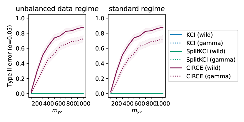
(b) Type II error.

Figure 6: Type I/II error comparison between the Gamma approximation and wild bootstrap methods of $p$-value estimation. Task 1 (Gaussian kernel) with the significance level $\alpha=0.05$.

B.2 GCM

The Generalised Covariance Measure (GCM, Shah and Peters, 2020) relies on estimates of the conditional mean

$$\widehat{f}(Z)\approx\mathbb{E}\left[X\,|\,Z\right]\,,\quad\widehat{g}(Z)\approx\mathbb{E}\left[Y\,|\,Z\right]\,.$$

For $n$ samples $x_{i}\in\mathbb{R}^{d_{x}}$ and $y_{i}\in\mathbb{R}^{d_{y}}$, define

$$R_{ikl}\, =(x_{i}-f(z_{i})))_{k}(y_{i}-g(z_{i}))_{l}\,,\quad\bar{R}_{kl}=\frac{1}{n}\sum_{i=1}^{n}R_{ikl}\,,\quad T_{kl}=\frac{\sqrt{n}\bar{R}_{kl}}{\sqrt{\frac{1}{n}\sum_{j=1}^{n}(R_{j})_{kl}^{2}-(\bar{R}_{kl})^{2}}}\,.$$

For 1-dimensional $X$ and $Y$ (and arbitrary $Z$), the $p$-value is computed as $p=2\,(1-\Phi(|T_{11}|))$ for the standard normal CDF $\Phi$.

For higher-dimensional $X$ and $Y$ (with $d_{x}d_{y}\geq 3$), the statistic becomes $S=\max_{k,l}|T_{kl}|$, and the $p$-value is computed by approximating the null distribution of $T_{kl}$ as a zero-mean Gaussian with the covariance matrix (for a $n$-dimensional vector $R^{kl}$ corresponding to all data points and dimensions $k,l$)

$$\Sigma_{kl,pd}=\frac{\frac{1}{n}\sum_{i=1}^{n}R_{ikl}R_{ipd}-\bar{R}_{kl}\bar{R}_{pd}}{\sqrt{\frac{1}{n}\sum_{i=1}^{n}R_{ikl}^{2}-\bar{R}_{kl}^{2}}\sqrt{\frac{1}{n}\sum_{i=1}^{n}R_{ipd}^{2}-\bar{R}_{pd}^{2}}}\,.$$

B.3 RBPT2

The Rao-Blackwellized Predictor Test (Polo et al., 2023; “2” stands for the test variant that doesn’t require approximation of $P(Y\,|\,Z)$) first trains a predictor $g(Y,Z)$ of $X$, e.g. by computing $g(Y,Z)\approx\mathbb{E}\left[X\,|\,Y,Z\right]$. (The original paper used a linear regression; we test this setup and also a CME with a Gaussian kernel.) Then, it builds a second predictor through CME as $h(Z)=\mathbb{E}\left[g(Y,Z)\,|\,Z\right]$ (the original paper used a polynomial kernel of degree two; we obtain similar results for a Gaussian kernel for linear $g$ and a set of Gaussian/polynomial kernels for a Gaussian $g$). Then, for a convex loss $l$, the test statistic $S$ is computed as

$$T_{i}=l(h(z_{i}),x_{i})-l(g(y_{i},z_{i}),x_{i})\,,\quad S=\frac{\sqrt{n}\sum_{i=1}^{n}T_{i}}{\sqrt{\sum_{i=1}^{n}T_{i}^{2}-(\sum_{i=1}^{n}T_{i})^{2}}}\,.$$

The $p$-value is then computed as $p=1-\Phi(S)$ (one-sided test); the basic intuition is that if $Y$ has no extra information about $X$ apart from the joint $Z$-dependence, the second predictor $h$ will perform as well as the first one $g$.

For Polo et al. (2023), the loss (for one-dimensional $X,Y$) was the mean squared error loss $l(g,x)=(g-x)^{2}$. For $d_{x}$-dimensional $x$, we also used the MSE loss $l(g,x)=\|g-x\|_{2}^{2}$ and found the test to consistently produce much lower Type I error than the nominal level $\alpha$ (Figure 7, black line), indicating that the statistic $S$ doesn’t follow a standard normal distribution. We argue that this happens due to the CME estimation error, and propose a debiased version of RBPT2 (which computes correct $p$-values; Figure 7, orange line):

Theorem 5.

For $g(Y,Z)$ approximated through CME, denote the approximation error as $\delta g$:

$$g(Y,Z)=\mathbb{E}\left[X\,|\,Y,Z\right]+\delta g(Y,Z)\,.$$

Assume that the second regression $h$ uses much more data (i.e. the unbalanced data regime in the main text) and so correctly estimates $h=\mathbb{E}\left[g(Y,Z)\,|\,Z\right]$, and that RBPT2 uses the MSE loss $l$.

Then, under $\mathrm{H}_{0}$, the unnormalized test statistic $T(X,Y,Z)=\|h(Z)-X\|_{2}^{2}-\|g(Y,Z)-X\|_{2}^{2}$ has a negative bias:

$$\mathbb{E}\left[T(X,Y,Z)\right]=_{\mathrm{H}_{0}}-\mathbb{E}\left[\|g(Y,Z)-h(Z)\|_{2}^{2}\right].$$

Proof.

Under $\mathrm{H}_{0}$, we have that

$$g(Y,Z)\, =\mu_{X\,|\,YZ}(Y,Z)+\delta g(Y,Z)=_{\mathrm{H}_{0}}\mu_{X\,|\,Z}(Z)+\delta g(Y,Z)\,,$$

$$\quad h(Z)\, =\mu_{X\,|\,Z}(Z)+\mathbb{E}\left[\delta g(Y,Z)\,|\,Z\right]=\mu_{X\,|\,Z}(Z)+\mu_{\delta g}(Z)\,.$$

We can therefore decompose the loss difference as

$$\|h(Z)-X\|_{2}^{2}-\|g(Y,Z)-X\|_{2}^{2}=_{\mathrm{H}_{0}}\|\mu_{X\,|\,Z}(Z)-X+\mu_{\delta g}(Z)\|_{2}^{2}-\|\mu_{X\,|\,Z}(Z)-X+\delta g(Y,Z)\|_{2}^{2}$$

$$\qquad=2\,(\mu_{X\,|\,Z}(Z)-X)^{\top}\mu_{\delta g}(Z)+\|\mu_{\delta g}(Z)\|_{2}^{2}-2\,(\mu_{X\,|\,Z}(Z)-X)^{\top}\delta g(Y,Z)-\|\delta g(Y,Z)\|_{2}^{2}\,.$$

We can take the expectation of this difference under $\mathrm{H}_{0}$, zeroing out the cross-product terms since $X\perp\!\!\!\perp Y\,|\,Z$:

$$\mathbb{E}\left[\|h(Z)-X\|_{2}^{2}-\|g(Y,Z)-X\|_{2}^{2}\right]\, =_{\mathrm{H}_{0}}-\mathbb{E}\left[\|\delta g(Y,Z)\|_{2}^{2}-\|\mu_{\delta g}(Z)\|_{2}^{2}\right]$$

$$=-\mathbb{E}\left[\|\delta g(Y,Z)-\mu_{\delta g}(Z)\|_{2}^{2}\right]=-\mathbb{E}\left[\|g(Y,Z)-h(Z)\|_{2}^{2}\right]\,.$$

∎

Conveniently, we can estimate this bias from the $g,h$ estimates, resulting in a bias-corrected RBPT2 (called RBPT2’ in the main text) with a test statistic

$$T_{i}=\|h(z_{i})-x_{i}\|_{2}^{2}-\|g(y_{i},z_{i})-x_{i}\|_{2}^{2}+\|g(y_{i},z_{i})-h(z_{i})\|_{2}^{2}\,.$$

While the derivation holds under the null, we note that adding a positive term to $T_{i}$ should decrease Type II errors since we’re testing for large positive deviations in $T_{i}$.

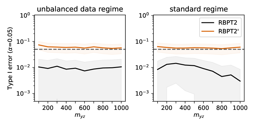
(a) Type I error, $n=100$.

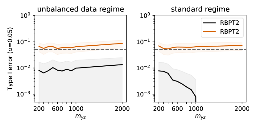
(b) Type I error, $n=200$.

Figure 7: Type I error, Task 1 (Gaussian kernel) with the significance level $\alpha=0.05$. Gray dashed line: $\alpha$. RBPT2 (black) vs its unbiased version RBPT2’ (orange). For both methods, Type II error remained at 0 (not shown).

Appendix C Experimental details and additional experiments

In all cases, we ran wild bootstrap 1000 times to estimate $p$-values. For kernel ridge regression, the $\lambda$ values were chosen (via leave-one-out) from $[10\,\delta,\dots,10^{7}\delta]$ (log scale) for SVD tolerance $\delta=\|K_{Z}\|_{2}\,\epsilon$ and machine precision $\epsilon$ (for float32 values).

For the experiments with artificial data with KCI, SplitKCI, and CIRCE, the kernels over $X$ and $Y$ were Gaussian $k(x,x^{\prime})=\exp(-\|x-x^{\prime}\|_{2}^{2}/\sigma^{2})$ (note that $\sigma^{2}$ is not multiplied by two in our implementation) with $\sigma^{2}=1$ (Tasks 1 and 3) or sample variance over the train set (Tasks 2 and 4; due to a different data scale in those tasks). The kernel over $Z$ for $\mu_{Y\,|\,Z}$ was always Gaussian, with $\sigma^{2}$ chosen (via leave-one-out) from $[0.5,1.0,2.0,5.0]$. For the experiments with the Gaussian kernel for $\mu_{X\,|\,Z}$, $\sigma^{2}$ was chosen from the same values. For the best kernel experiments, we also used LOO and additionally chose from polynomial kernels $k_{p}(z,z^{\prime})=(z^{\top}z^{\prime}+c)^{k}$ ($c$ from $[0.1,0.2,\dots,1.0]$, $k$ from $[1,2,\dots,6]$) and normalized polynomial kernels $k_{np}(z,z^{\prime})=(\alpha\,z^{\top}z^{\prime}/\|z\|_{2}\|z^{\prime}\|_{2}+1)^{k}/(1+\alpha)^{k}$ ($\alpha$ from $[0.0,0.2,\dots,1.0]$, $k$ from $[1,2,\dots,6]$; $\alpha=0$ would essentially avoid conditioning, and the CME estimator would be removed during centering with $H$). For GCM, we use the same setup for $\widehat{f}(Z)\approx\mathbb{E}\left[X\,|\,Z\right]\,,\widehat{g}(Z)\approx\mathbb{E}\left[Y\,|\,Z\right]$ (see the definitions in Section B.2). For RBPT2, in the experiments with the Gaussian kernel we used the linear kernel for $g(Y,Z)$ and the Gaussian kernel for $h(Z)$ with the same parameter choice (see the definitions in Section B.3). For the best kernel experiments, we used the Gaussian kernel with $\sigma^{2}=1$ for $g$ and the aforementioned list of three kernels for $h$. This was done to reflect the increased model flexibility in other measures; in the original experiments of Polo et al. (2023), $g$ was found through (non-ridge) regression and $h$ used a polynomial kernel of degree 2. We found this setup to be similar to our first setup in our preliminary experiments (not shown). For all runs, the $p$-values were computed with $n_{i}=100$ samples of the train set (indexed by $i$) and (for each train set) $n_{j}=100$ samples of the test set (indexed by $j$), and converted to accept/reject binary variables $p_{ij}$. We then plotted the mean value $\mu=\frac{1}{n_{i}n_{j}}\sum_{ij}p_{ij}$ (which is a standard mean estimate) and the sample variance through the law of total variance as $\sigma^{2}=\frac{1}{n_{i}}\sum_{i}\sigma_{i}^{2}+\frac{1}{n_{i}}(\mu_{i}-\mu)^{2}$ for sample mean $\mu_{i}$ and variance $\sigma^{2}_{i}$ estimators over train set $i$, since $p_{ij}$ depends on $i$ across $j$. As an estimate to standard error, we used $\sigma/\sqrt{n_{i}}$ in the plots (this would be exact for $n_{j}\rightarrow\infty$). We opted out for this method since the Type I error estimate remains unbiased, but re-evaluating the test statistic for new test data becomes computationally significantly cheaper.

For the car insurance data, we followed exactly the same procedure as Polo et al. (2023) for RBPT, RBPT2, RBPT2’ and GCM. For kernel-based measures and the simulated $\mathrm{H}_{0}$, the kernel over $X$ was Gaussian with $\sigma^{2}$ determined from sample variance over train data; the kernel over $Y$ was a simple $k_{y}(y,y^{\prime})=\mathbb{I}[y=y^{\prime}]$ since $Y$ is binary; the kernel over $Z$ was Gaussian with $\sigma^{2}$ chosen from $[0.5,1.0,2.0]\cdot\widehat{\sigma}^{2}$ for train sample variance $\widehat{\sigma}^{2}$. For the actual $p$-values, we split the train data in two randomly for independent $\mu_{X\,|\,Z}$ and $\mu_{Y\,|\,Z}$ regression (to avoid the high memory requirements of the full dataset). The rejection indicators $p_{ij}$ for seed $i$ for the simulated $\mathrm{H}_{0}$ task were computed for each company $j$ individually. As in Polo et al. (2023), we did not make the variance correction through the law of total variance, essentially estimating average rejection rate across companies, since the companies are fixed and not sampled randomly. Therefore, the standard errors are correct (for this quantity).

For KCI, CIRCE and SplitKCI with the Gamma approximation, we used the biased HSIC-like estimator in Equation 5 (note that the Gamma approximation is derived for the biased one). For wild bootstrap, we used the unbiased HSIC estimator (Song et al., 2007) (the biased one performed marginally worse; not shown) for kernel matrices $K,L$:

$$\frac{1}{m(m-3)}\left(\mathrm{Tr}\,\left(KL\right)+\frac{1^{\top}K11^{\top}L1}{(m-1)(m-2)}-\frac{2}{m-2}1^{T}KL1\right)\,.$$ (17)

C.1 Artificial data

For Task 1, CIRCE requires significantly more data than all other methods to achieve the desired Type 1 error rates, and also suffers from large Type 2 errors for both $n=100$ (Figures 8(a) and 8(b)) and $n=200$ (Figures 8(c) and 8(d)) test set sizes.

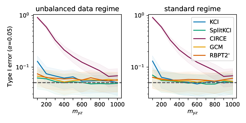
(a) Type I error, $n=100$.

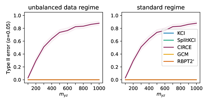
(b) Type II error, $n=100$.

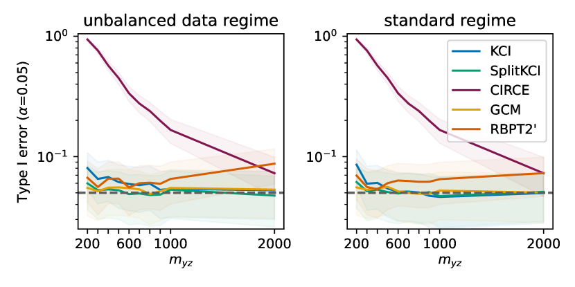
(c) Type I error, $n=200$.

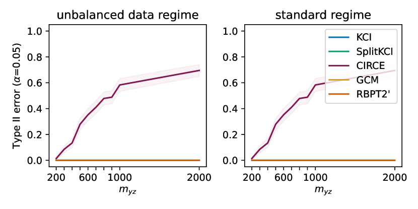
(d) Type II error, $n=200$.

Figure 8: Task 1 (Gaussian kernel) with the significance level $\alpha=0.05$. Gray dashed line: $\alpha$. Left panel: unbalanced data regime ($n=m_{xz}$, growing $m_{yz}$). Right panel: standard data regime (fixed $n$, growing $m_{xz}=m_{yz}$).

For Task 2, increasing the number of test data points improves Type II errors for KCI and SplitKCI (Figure 9(d)). In addition, increasing the pool of $Z$-kernels helps RBPT2’ achieve lower (albeit still higher than for KCI and SplitKCI) Type 2 errors (Figures 10(b) and 10(d)).

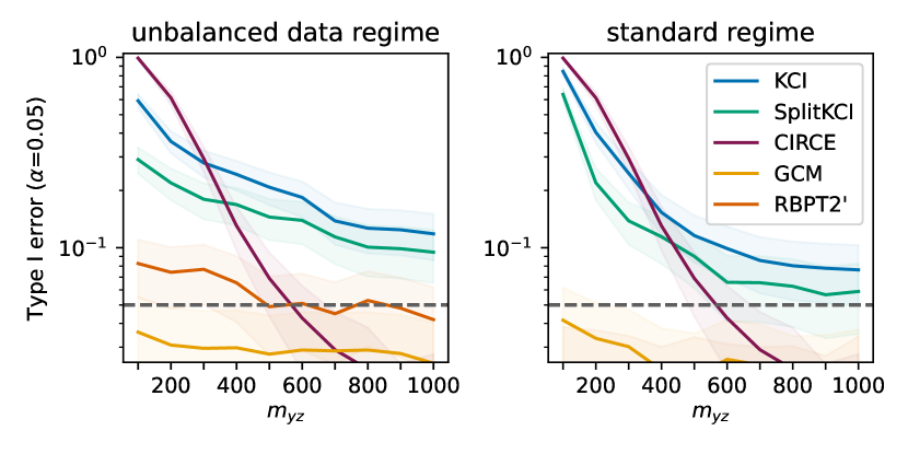
(a) Type I error, $n=100$.

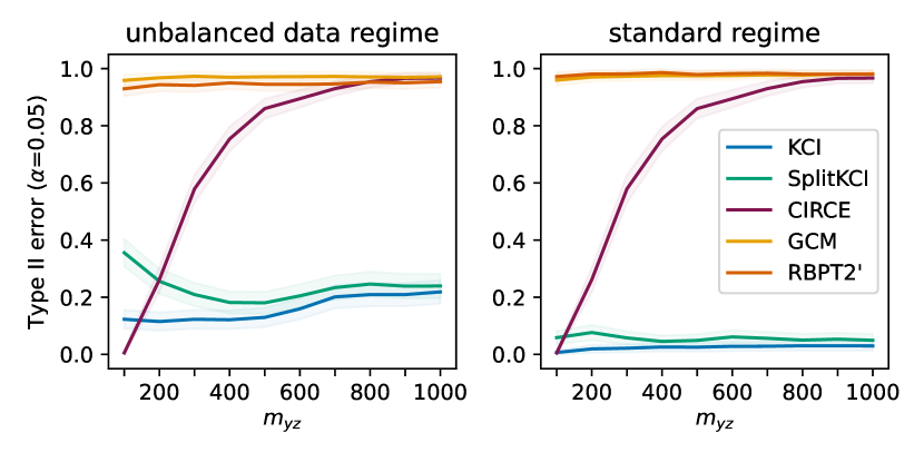
(b) Type II error, $n=100$.

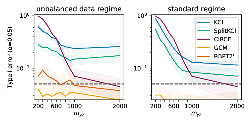
(c) Type I error, $n=200$.

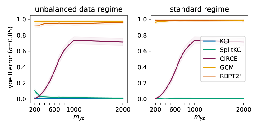
(d) Type II error, $n=200$.

Figure 9: Task 2 (Gaussian kernel) with the significance level $\alpha=0.05$. Gray dashed line: $\alpha$. Left panel: unbalanced data regime ($n=m_{xz}$, growing $m_{yz}$). Right panel: standard data regime (fixed $n$, growing $m_{xz}=m_{yz}$).

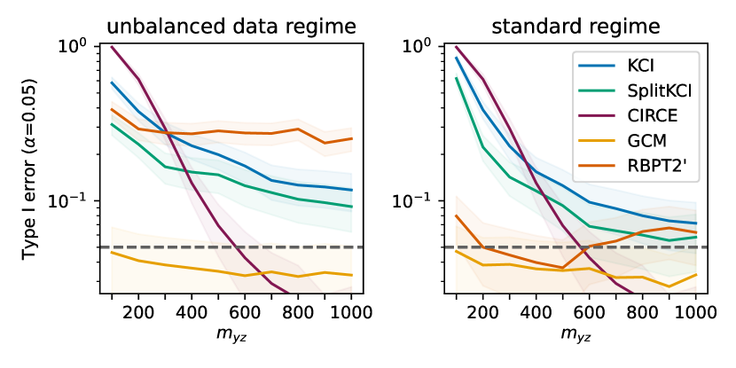
(a) Type I error, $n=100$.

(b) Type II error, $n=100$.

(c) Type I error, $n=200$.

(d) Type II error, $n=200$.

Figure 10: Task 2 (best $Z$-kernel for $X\,|\,Z$) with the significance level $\alpha=0.05$. Gray dashed line: $\alpha$. Left panel: unbalanced data regime ($n=m_{xz}$, growing $m_{yz}$). Right panel: standard data regime (fixed $n$, growing $m_{xz}=m_{yz}$).

Task 3 results for all setups follow the trend presented in the main text, and are summarized in Figures 11 and 12.

(a) Type I error, $n=100$.

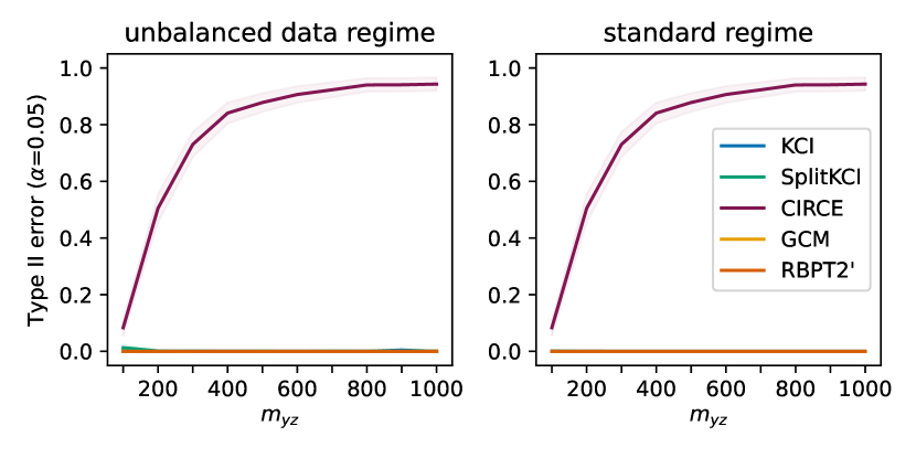
(b) Type II error, $n=100$.

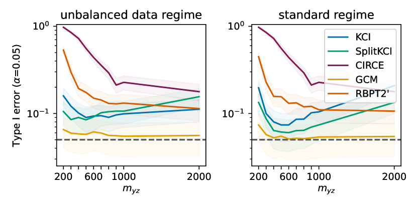
(c) Type I error, $n=200$.

(d) Type II error, $n=200$.

Figure 11: Task 3 (Gaussian kernel) with the significance level $\alpha=0.05$. Gray dashed line: $\alpha$. Left panel: unbalanced data regime ($n=m_{xz}$, growing $m_{yz}$). Right panel: standard data regime (fixed $n$, growing $m_{xz}=m_{yz}$).

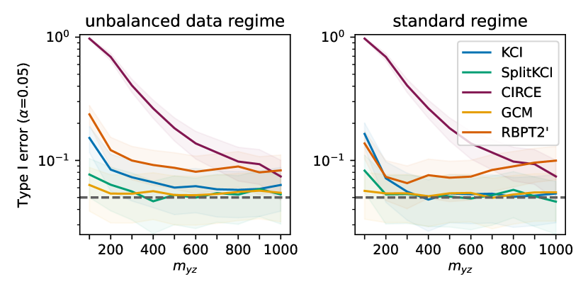
(a) Type I error, $n=100$.

(b) Type II error, $n=100$.

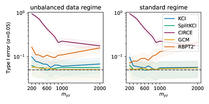
(c) Type I error, $n=200$.

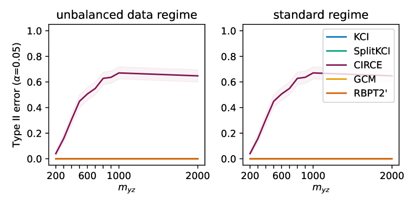
(d) Type II error, $n=200$.

Figure 12: Task 3 (best $Z$-kernel for $X\,|\,Z$) with the significance level $\alpha=0.05$. Gray dashed line: $\alpha$. Left panel: unbalanced data regime ($n=m_{xz}$, growing $m_{yz}$). Right panel: standard data regime (fixed $n$, growing $m_{xz}=m_{yz}$).

For Task 4, using a linear kernel for $g$ and Gaussian kernel for $h$ in RBPT2’ led to worse Type I errors (Figure 13(a)) compared to a Gaussian $g$/best of several kernel $h$ in the main text (Figure 4). Surprisingly, CIRCE performed the best overall, suggesting that the $X\,|\,Z$ regression is much harder than the $Y\,|\,Z$ one, leading to better results for CIRCE since it avoids the former completely.

C.2 Real data

For the car insurance data (full dataset, i.e. merged for all companies), we compute the $p$-values as in Polo et al. (2023). The train/test split of the dataset is done as 70/30%. For KCI and SplitKCI, we further split the train set in half for each $\mu_{X\,|\,Z}$ and $\mu_{Y\,|\,Z}$ regression due to increased memory requirements compared to other methods. The results are summarized in Figure 13(b), suggesting that most methods, apart from RBPT and RBPT2, reject the null at $\alpha=0.05$ for all states. CIRCE (not shown in the main text) performed similar to KCI/SplitKCI but produced less accurate Type 1 errors.

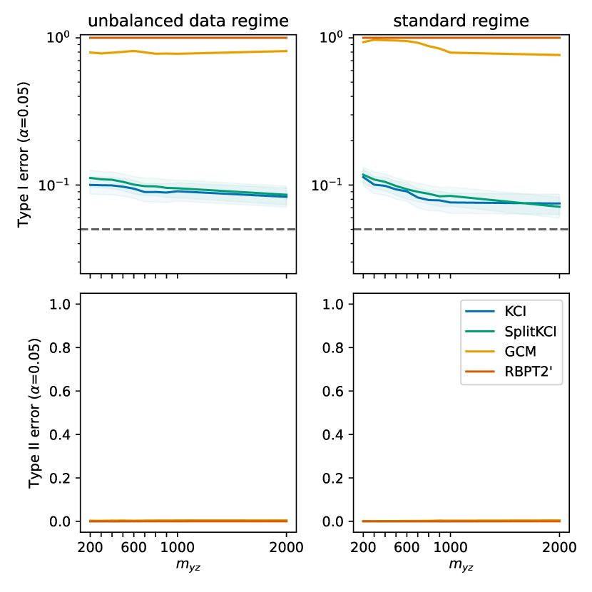
(a) Task 4, Type I error for $\alpha=0.05$ with $d=40$ and Gaussian $Z$-kernel.

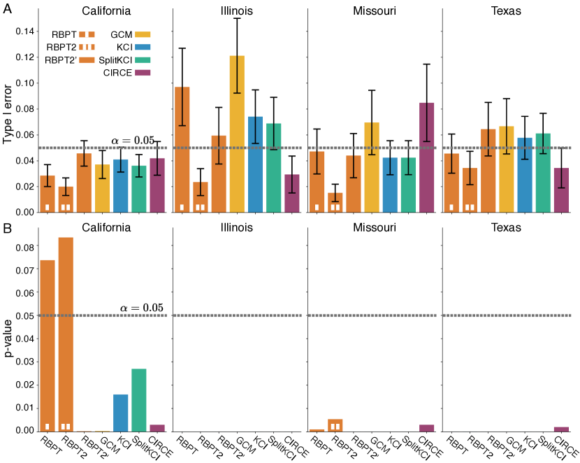
(b) Car insurance dataset; expanded from Polo et al. (2023). RBPT(2): Polo et al. (2023); GCM: Shah and Peters (2020); KCI: Zhang et al. (2011); CIRCE: Pogodin et al. (2022); SplitKCI: ours. A. Simulated null. B. Test performance on the full dataset.