Non-local time evolution equation with singular integral and its application to traffic flow model

Abstract

We consider an integro-differential equation model for traffic flow which is an extension of the Burgers equation model. To discuss the model, we first examine general settings for integrable integro-differential equations and find that they are obtained through a simple residue formula from integrable eqations in a complex domain. As demonstration of the efficiency of this approach, we list several integrable equations including a difference equation with double singular integral and an equation with elliptic singular integral. Then, we discuss the traffic model with singular integral and show that the model exhibits interaction between free flow region and congested region depending on the parameter of non-locality.

1 Introduction

In dynamics of natural or social phenomena, non-local effect often plays an important role and has to be represented adequately for mathematical modeling. Integro-differential equations are an effective tool for this purpose and have been used in fields such as fluid mechanics, electric circuits, and epidemiology. A notable example in fluid dynamics is the intermediate long wave (ILW) equation which describes long internal gravity waves in a stratified fluid with finite depth [Kubota][RIJoseph_1977]:

$$\begin{cases}&\displaystyle\partialderivative{u(x,t)}{t}+\frac{1}{\delta}\partialderivative{u(x,t)}{x}+2u(x,t)\partialderivative{u(x,t)}{x}+T\left(\partialderivative[2]{u(x,t)}{x}\right)=0,\\[3.0pt] &\displaystyle T\left(v(x,t))\right):=\frac{-1}{2\delta}\mathchoice{{\vbox{\hbox{$\textstyle-$}}\kern-4.86108pt}}{{\vbox{\hbox{$\scriptstyle-$}}\kern-3.25pt}}{{\vbox{\hbox{$\scriptscriptstyle-$}}\kern-2.29166pt}}{{\vbox{\hbox{$\scriptscriptstyle-$}}\kern-1.875pt}}\!\int_{-\infty}^{\infty}\coth{\frac{\pi}{2\delta}(x-x^{\prime})}v(x^{\prime},t)\,dx^{\prime}.\end{cases}$$ (1.1)

An important property of ILW eq. (1.1) is that it has $N$ soliton solutions, infinite number of conserved quantities, Bäcklund transformation, and that initial value problems can be solved by inverse scattering transform (IST)[RIJoseph_1977][Satsuma][Kodama1982]. Namely, it is a nonlinear integrable equation. In fact, by taking the limit $\delta\to 0$, (1.1) turns to the celebrated Korteweg deVries (KdV) equation and, by $\delta\to+\infty$, it turns to Benjamin-Ono equation[Benjamin1967][Ono1975].

To obtain the solutions and conserved quantities for (1.1), IST schemes were used and its associated spectral problems turned out to be the Riemann-Hilbert (RH) boundary value problem[Kodama1982]. Other RH problems have been introduced and integro-differential equations related to well-known integrable equations such as non-linear Schrödinger equation[ZakharovShabat1972], Modified Korteweg-deVries equation[Wadachi1972], sine-Gordon equation[Hirota1971] and Kadomtsev-Petiviashuvili equation[KadomtsevPetviashvili1970] have been constructed[DegasperisSantini1983]. The method is to obtain solutions of a RH boundary value problem, $\psi(z)$ ($z\in\mathbb{C}$) which satisfy a certain constraint such as $\psi(x)=-\psi(x+2\mathrm{i}\delta)$ $(x\in\mathbb{R})$, and consider evolution equations which preserve the constraint. Most of these integrable integro-differential equations are expressed with singular integral as in (1.1).

This approach with RH problems can be extended to an infinite series of integrable integro-differential equations, that is, integro-differential hierarchies of ILW, Sine-Gordon and AKNS equations [DegasperisSantini1983][DegasperisSantiniAblowitz1985][SantiniAblowitzFokas1987]. Another approach to construct the integro-differential analogue of ILW hierarchy and that of Intermediate nonlinear Schrödinger equation hierarchy was proposed [TutiyaSatsuma2003] on the basis of the theory of KP hierarchy[Sato]. In Ref. [TutiyaSatsuma2003], additional discrete flow in applied to the KP hierarchy and the compatibility condition of the two flows are proved to give these integro-differential hierarchies.

Recently, Satsuma and Tomoeda proposed an integro-differential equation which describes time evolution of traffic density $\rho(x,t)$ as

$$\frac{\partial\rho}{\partial t}=V_{\max}\left(\mathchoice{{\vbox{\hbox{$\textstyle-$}}\kern-4.86108pt}}{{\vbox{\hbox{$\scriptstyle-$}}\kern-3.25pt}}{{\vbox{\hbox{$\scriptscriptstyle-$}}\kern-2.29166pt}}{{\vbox{\hbox{$\scriptscriptstyle-$}}\kern-1.875pt}}\!\int_{-\infty}^{\infty}\coth\frac{\pi}{2\delta}(x-y)\frac{\partial\rho}{\partial y}(y)dy+I-\rho_{\max}\right)\frac{\partial\rho}{\partial x}+D\frac{\partial^{2}\rho}{\partial x^{2}}.$$ (1.2)

Here $V_{\max}$ is the maximum velocity of a car, $\rho_{\max}$ is the density of the deadlock phenomenon, $\rho(\pm\infty,t)$ are assumed to be constant in time $t$ and $I:=\rho(\infty,t)+\rho(-\infty,t)$. Equation (1.2) is an extension of the equation:

$$\frac{\partial\rho}{\partial t}=-V_{\max}\left(1-2\frac{\rho}{\rho_{\max}}\right)\frac{\partial\rho}{\partial x}+D\frac{\partial^{2}\rho}{\partial x^{2}}$$ (1.3)

which is a Burgers equation for a mathematical model of traffic flow based on fluid dynamics[Lighthill-Whitham][Whitham] In fact,

$$\lim_{\delta\to+0}\mathchoice{{\vbox{\hbox{$\textstyle-$}}\kern-4.86108pt}}{{\vbox{\hbox{$\scriptstyle-$}}\kern-3.25pt}}{{\vbox{\hbox{$\scriptscriptstyle-$}}\kern-2.29166pt}}{{\vbox{\hbox{$\scriptscriptstyle-$}}\kern-1.875pt}}\!\int_{-\infty}^{\infty}\coth\frac{\pi}{2\delta}(x-y)\frac{\partial\rho}{\partial y}(y)dy =\mathchoice{{\vbox{\hbox{$\textstyle-$}}\kern-4.86108pt}}{{\vbox{\hbox{$\scriptstyle-$}}\kern-3.25pt}}{{\vbox{\hbox{$\scriptscriptstyle-$}}\kern-2.29166pt}}{{\vbox{\hbox{$\scriptscriptstyle-$}}\kern-1.875pt}}\!\int_{-\infty}^{\infty}\mathrm{sgn}\,(x-y)\frac{\partial\rho}{\partial y}(y)dy$$

$$=2\rho(x)-\rho(\infty)-\rho(-\infty),$$

and (1.2) turns to (1.3). Equation (1.2) was first investigated in Ref.[Satsuma-Mimura] in an equivalent form as

$$\frac{\partial u}{\partial t}=-\frac{\partial}{\partial x}\left(T(u)\cdot u\right)+D\partialderivative[2]{u}{x},$$

where one soliton solution has been obtained by Hirota’s bilinear method and extension to periodic solutions have been discussed.

Motivated by the application of the singular integral equation to traffic flow problems, this paper firstly considers integrable integro-differential equations and their general solutions as reductions from the well-established equations. It is based on analytic properties of the solutions in a complex domain using fundamental residue formula. Although this approach is essentially equivalent to that with the RH problem, we need not consider the compatibility condition between the evolution equation and the constraint on the solutions appearing in the RH problem, because the solution of integrable differential or difference equations in the complex domain can be obtained directly, and it turns into a solution in the range of the real axis of the corresponding intego-differential equation. As a natural extension of our approach, we show that the singular integral $T\left(v(x,t))\right)$ can be generalized to that with elliptic function. Then, we apply the method to the traffic flow model (1.2) and discuss the interaction between free-flow and congested regions which depend on the parameter of non-locality. The structure of this paper is as follows: First, in Section 2, we discuss the integral representation of holomorphic functions and their relationship with boundary values. Using this correspondence, we clarify the connection between systems in a domain and those on the boundary, leading us to naturally observe the emergence of singular integrals. In Section 3, we tackle specific examples. We extend representative integrable systems, such as the KdV equation and the Toda equation, to equations that incorporate singular integrals, then, using these approach, we examine the traffic flow model in Section LABEL:sect:traffic_flow. In the final section, we offer concluding remarks.

2 Singular integral and residue formula

In this section, we apply residue formula to establish the relation between singular integral and difference operator for an analytic complex functions. Hereafter we often represent partial derivatives using subscripts and omit the dependent variables $(x,t)$. For instance, $\frac{\partial^{2}u}{\partial x^{2}}(x,t)$ is denoted as $u_{2x}$. As an example, let us consider the integro-differential equation

$$u_{t}+u_{3x}-6T(u_{x})u_{x}=0,$$ (2.1)

where $T$ denotes a singular integral operator, and it acts on a function $v$ as

$$Tv(x):=\frac{-1}{2\delta}\mathchoice{{\vbox{\hbox{$\textstyle-$}}\kern-4.86108pt}}{{\vbox{\hbox{$\scriptstyle-$}}\kern-3.25pt}}{{\vbox{\hbox{$\scriptscriptstyle-$}}\kern-2.29166pt}}{{\vbox{\hbox{$\scriptscriptstyle-$}}\kern-1.875pt}}\!\int_{-\infty}^{\infty}\coth{\frac{\pi}{2\delta}(x-x^{\prime})}v(x^{\prime})\,dx^{\prime}.$$ (2.2)

This equation is an extension of a nonlinear partial differential equation with a dispersion term to have nonlinear non-local effects, and can be obtained through Riemann-Hilbert problem related to potential KdV equation [Santini_review]. To show effectiveness of our approach, though it is simple, we examine (2.1) in some detail.

2.1 Equations obtained in the limit of the parameter $\delta$

We show that Eq. (2.1) reduces to the KdV equation in the limit $\delta\rightarrow+0$. Let us rescale $u$ as $\tilde{u}(x,t):=u(x,t)/\delta$. We denote $\tilde{u}$ as $u$ again, and impose the boundary condition $u\,\rightarrow\,0\quad\text{as}\quad|x|\rightarrow\infty$. By taking the limit $\delta\rightarrow+0$, the nonlinear term of (2.1) becomes

$$-6\delta(Tu_{x})u_{x} \rightarrow 3\left(\int_{-\infty}^{x}u_{x}(x^{\prime})\,dx^{\prime}-\int_{x}^{\infty}u(x^{\prime})_{x}\,dx^{\prime}\right)u_{x}$$

$$=3(u(x)-u(-\infty)-u(\infty)+u(x))u_{x}$$

$$=6uu_{x},$$

where we used the relation $\coth\frac{\pi}{2\delta}x\rightarrow\text{sgn}(x)$. Therefore, in the limit $\delta\rightarrow+0$, it reduces to the KdV equation. On the other hand, in the limit $\delta\rightarrow\infty$, we have

$$\frac{-1}{2\delta}\coth\frac{\pi}{2\delta}x =\frac{-1}{\pi}\frac{1+\mathcal{O}\left(\frac{1}{\delta^{2}}\right)}{x+\mathcal{O}\left(\frac{1}{\delta^{3}}\right)}$$ (2.3)

$$\rightarrow\frac{-1}{\pi}\frac{1}{x}.$$ (2.4)

Using the Hilbert transform defined by

$$\mathcal{H}v(x):=\frac{1}{\pi}\mathchoice{{\vbox{\hbox{$\textstyle-$}}\kern-4.86108pt}}{{\vbox{\hbox{$\scriptstyle-$}}\kern-3.25pt}}{{\vbox{\hbox{$\scriptscriptstyle-$}}\kern-2.29166pt}}{{\vbox{\hbox{$\scriptscriptstyle-$}}\kern-1.875pt}}\!\int_{-\infty}^{\infty}\frac{v(x^{\prime})\,dx^{\prime}}{x-x^{\prime}},$$ (2.5)

the equation reduces to

$$u_{t}+u_{3x}+6(\mathcal{H}u_{x})u_{x}=0.$$ (2.6)

Since both limits give integrable equations, we expect that (2.1) is also an integrable equation as the ILW equation (1.1). In fact, we shall see in the following subsections that it is obtained from the KdV equation on a complex plane by imposing a solution to be holomorphic in a stripe domain.

2.2 Holomorphic function in a complex domain and its boundary values

Proposition 2.1.

We consider the complex domain $D:=\{z|-\delta<\operatorname{Im}z<\delta\}$. Let $U$ be holomorphic function in $D$ and Hölder continuous on $\partial D$. We denote $z=x+\mathrm{i}y$ $(x,\,y\in\mathbb{R})$ and assume that

$$\lim_{{x\to\pm\infty}}U(x+\mathrm{i}y) =U_{\pm\infty}\quad(\forall y),$$ (2.7)

where $U_{\pm\infty}$ are constants. Then the following relation holds.

$$U(x+\mathrm{i}\delta)+U(x-\mathrm{i}\delta)-U_{\infty}-U_{-\infty} =-\frac{1}{\mathrm{i}}T\left(U(x+\mathrm{i}\delta)-U(x-\mathrm{i}\delta)\right)$$ (2.8)

Proof.

Let us consider the following complex integral:

$$\oint_{C}\frac{1}{2\delta}\tanh\left[\frac{\pi}{2\delta}(x-z)\right]\,f(z)\,dz$$ (2.9)

The integration path is shown in Figure 1.

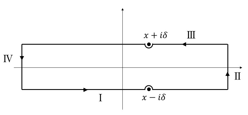
Figure 1: Integration path $C$

Let the constant $\delta>0$ and assume that $U(z)$ has no singularities on $\operatorname{Im}z=\pm\delta$ and the singularities inside the contour are only poles.

Given that

$$\tanh\frac{\pi}{2\delta}(x-y+\mathrm{i}\delta)=\coth\frac{\pi}{2\delta}(x-y)$$ (2.10)

and near $x-y\sim 0$, $\coth\frac{\pi}{2\delta}(x-y)\sim\frac{2\delta}{\pi(x-y)}$, we deduce

$$\int_{I} \rightarrow\mathchoice{{\vbox{\hbox{$\textstyle-$}}\kern-4.86108pt}}{{\vbox{\hbox{$\scriptstyle-$}}\kern-3.25pt}}{{\vbox{\hbox{$\scriptscriptstyle-$}}\kern-2.29166pt}}{{\vbox{\hbox{$\scriptscriptstyle-$}}\kern-1.875pt}}\!\int_{-\infty}^{\infty}\coth\left[\frac{\pi}{2\delta}(x-y)\right]\,U(y-\mathrm{i}\delta)\,dy+2\mathrm{i}\delta U(x-\mathrm{i}\delta)$$ (2.11)

$$\int_{I\!I\!I} \rightarrow-\mathchoice{{\vbox{\hbox{$\textstyle-$}}\kern-4.86108pt}}{{\vbox{\hbox{$\scriptstyle-$}}\kern-3.25pt}}{{\vbox{\hbox{$\scriptscriptstyle-$}}\kern-2.29166pt}}{{\vbox{\hbox{$\scriptscriptstyle-$}}\kern-1.875pt}}\!\int_{-\infty}^{\infty}\coth\left[\frac{\pi}{2\delta}(x-y)\right]\,U(y+\mathrm{i}\delta)\,dy+2\mathrm{i}\delta U(x+\mathrm{i}\delta)$$ (2.12)

From the assumption, we have

$$\int_{I\!I}\ \rightarrow\ -2\mathrm{i}\delta U_{\infty},\qquad\qquad\int_{I\!V}\ \rightarrow\ -2\mathrm{i}\delta U_{-\infty}$$ (2.13)

Thus, we obtain

$$\mathchoice{{\vbox{\hbox{$\textstyle-$}}\kern-4.86108pt}}{{\vbox{\hbox{$\scriptstyle-$}}\kern-3.25pt}}{{\vbox{\hbox{$\scriptscriptstyle-$}}\kern-2.29166pt}}{{\vbox{\hbox{$\scriptscriptstyle-$}}\kern-1.875pt}}\!\int_{-\infty}^{\infty}\coth\left[\frac{\pi}{2\delta}(x-y)\right]\,\left\{U(y-\mathrm{i}\delta)-U(y+\mathrm{i}\delta)\right\}\,dy$$

$$=-2\mathrm{i}\delta\left\{U(x+\mathrm{i}\delta)+U(x-\mathrm{i}\delta)-U_{\infty}-U_{-\infty}\right\}$$ (2.14)

which completes the proof. ∎

The following corollary immediately follows from prop 2.1.

Corollary 2.2.

When

$$U(x-\mathrm{i}\delta)=U^{*}(x+\mathrm{i}\delta)$$ (2.15)

$$U_{\infty}+U_{-\infty}=0$$ (2.16)

holds, writing $U(x+\mathrm{i}\delta)$ = : $w(x)+\mathrm{i}v(x)$, we have

$$w(x)=\mathchoice{{\vbox{\hbox{$\textstyle-$}}\kern-4.86108pt}}{{\vbox{\hbox{$\scriptstyle-$}}\kern-3.25pt}}{{\vbox{\hbox{$\scriptscriptstyle-$}}\kern-2.29166pt}}{{\vbox{\hbox{$\scriptscriptstyle-$}}\kern-1.875pt}}\!\int_{-\infty}^{\infty}\frac{-1}{2\delta}\coth\left[\frac{\pi}{2\delta}(x-y)\right]\,v(y)\,dy$$ (2.17)

2.3 Derivation of Eq. (2.1)

We show that Eq. (2.1) is derived from the complex KdV equation

$$U(z,t)_{t}+U(z,t)_{3z}+6U(z,t)U(z,t)_{z}=0.$$ (2.18)

on the domain $D$. Assume that $U(z,t)$ is a solution of the KdV equation on $D$ that satisfies the assumptions of corollary 2.2. Taking the limit of $U$ as $\operatorname{Im}z\rightarrow-\delta$ and using the real function $v(x,t)$, we have

$$U(x+\mathrm{i}\delta)=-Tv(x,t)+\mathrm{i}v(x,t)$$ (2.19)

which satisfies

$$(-Tv+\mathrm{i}v)_{t}+(-Tv+\mathrm{i}v)_{3x}+6(-Tv+\mathrm{i}v)(-Tv+\mathrm{i}v)_{x}=0.$$ (2.20)

Therefore, by extracting the imaginary part, we obtain

$$v_{t}+v_{3x}-6(vTv)_{x}=0.$$ (2.21)

By substituting $v=u_{x}$ and integrating once with respect to $x$, it yields (2.1).

2.4 Soliton solutions

Once the origin of the singular integral equation (2.1) is clarified as above, its properties such as general solutions, Lax pairs, and conserved quantities can be straightforwardly obtained from those of the KdV equation.

In this subsection, we discuss the solutions for (2.1). There are lots of established methods to construct the solutions of the KdV equation, such as inverse scattering methods, Hirota bilinear methods, reduction from the KP hierarchy. Here we consider $N$ soliton solutions using the tau function $\tau(z,t)$. The solution to the KdV equation is written using the tau function $\tau(z,t)$ as

$$U(z,t) =2\frac{\partial^{2}}{\partial z^{2}}\log\tau(z,t)$$ (2.22)

The $N$ soliton solutions are given as

$$\tau(z,t) =\sum_{\{\mu_{k}\}_{k=1}^{N}\in\{0,1\}^{N}}\exp{\sum_{i=1}^{N}\mu_{i}\eta_{i}+\sum_{1\leq i<j\leq N}\mu_{i}\mu_{j}A_{ij}},$$ (2.23)

where

$$\eta_{i} :=k_{i}z-k_{i}^{3}t-\theta_{i},\quad(i=1,2,...,N)$$

$$\mathrm{e}^{A_{ij}} :=\frac{(k_{i}-k_{j})^{2}}{(k_{i}+k_{j})^{2}}\quad(1\leq i<j\leq N),$$

for real parameters $k_{i}$ ($k_{i}\neq\pm k_{j}$ for $i\neq j$) and $\theta_{i}$. To ensure that the solution is holomorphic, it is sufficient to set $0<k_{j}\delta<\pi$ for any $j$.

Similar to the derivation of the equation, by taking a limit as $\operatorname{Im}z\rightarrow\delta$, taking its imaginary part, and integrating once with respect to $x$, the solution to (2.1) is expressed as

$$u =2\frac{\operatorname{Re}\tau(\operatorname{Im}\tau)_{x}-(\operatorname{Re}\tau)_{x}\operatorname{Im}\tau}{\operatorname{Re}\tau^{2}+\operatorname{Im}\tau^{2}}.$$ (2.24)

Specifically, we provide explicit expressions for the 1-soliton and 2-soliton solutions. For a 1-soliton, the $\tau$ function corresponding to $U$ is given by

$$\tau_{1}=1+\mathrm{e}^{kz-k^{3}t}$$ (2.25)

where $k\in\mathbb{R}$ and we set $\theta=0$. From the derived formula (2.24) we find that the solution is

$$u=\frac{k\sin{k\delta}}{\cosh{(kx-k^{3}t)}+\cos{k\delta}}.$$ (2.26)

Similarly, for a 2-soliton solution, the $\tau$ function that provides the solution $U$ is given by

$$\tau_{2}=1+\mathrm{e}^{k_{1}z-k_{1}^{3}t}+\mathrm{e}^{k_{2}z-k_{2}^{3}t}+\mathrm{e}^{(k_{1}+k_{2})z-(k_{1}^{3}+k_{2}^{3})t+A_{12}}$$ (2.27)

where $k_{1},k_{2}\in\mathbb{R}$ and $\mathrm{e}^{A_{12}}=\left(\frac{k_{1}-k_{2}}{k_{1}+k_{2}}\right)^{2}$. Instead of giving the concrete expression of the corresponding solution, let us discuss the asymptotic behavior of the solution corresponding to the 2-soliton solution as $t$ approaches $\pm\infty$. We assume $0<k_{1}<k_{2}$. Firstly let us consider a region $x-k_{1}^{2}t=const.$, that is, we consider a region where a soliton with wavelength $k_{1}$ exists. In this region, since $\mathrm{e}^{\eta_{2}}\gg\mathrm{e}^{\eta_{1}}$ as $t\to-\infty$, we have

$$\begin{cases}\operatorname{Re}\tau_{2}&\sim\mathrm{e}^{\eta_{2}}(\cos k_{2}\delta+a_{12}\mathrm{e}^{\eta_{1}}\cos(k_{1}+k_{2})\delta),\\ \operatorname{Im}\tau_{2}&\sim\mathrm{e}^{\eta_{2}}(\sin k_{2}\delta+a_{12}\mathrm{e}^{\eta_{1}}\sin(k_{1}+k_{2})\delta),\\ {\operatorname{Re}\tau_{2}}_{x}&\sim\mathrm{e}^{\eta_{2}}(k_{2}\cos k_{2}\delta+(k_{1}+k_{2})a_{12}\mathrm{e}^{\eta_{1}}\cos(k_{1}+k_{2})\delta),\\ {\operatorname{Im}\tau_{2}}_{x}&\sim\mathrm{e}^{\eta_{2}}(k_{2}\sin k_{2}\delta+(k_{1}+k_{2})a_{12}\mathrm{e}^{\eta_{1}}\sin(k_{1}+k_{2})\delta).\end{cases}$$ (2.28)

From (2.28), we obtain

$$u\sim\frac{k_{1}\sin k_{1}\delta}{\cosh(\eta_{1}+\alpha)+\cos k_{1}\delta},$$ (2.29)

where $\alpha:=2\log\frac{k_{2}-k_{1}}{k_{2}+k_{1}}$.

As $t\rightarrow\infty$, $\mathrm{e}^{\eta_{1}}\gg\mathrm{e}^{\eta_{2}}$ and $\mathrm{e}^{\eta_{2}}\rightarrow 0$, we find

$$\begin{cases}\operatorname{Re}\tau_{2}&\sim 1+\mathrm{e}^{\eta_{1}}\cos k_{1}\delta,\\ \operatorname{Im}\tau_{2}&\sim\mathrm{e}^{\eta_{1}}\sin k_{1}\delta,\\ {\operatorname{Re}\tau_{2}}_{x}&\sim k_{1}\mathrm{e}^{\eta_{1}}\cos k_{1}\delta,\\ {\operatorname{Im}\tau_{2}}_{x}&\sim k_{1}\mathrm{e}^{\eta_{1}}\sin k_{1}\delta.\end{cases}$$ (2.30)

From (2.30), we obtain

$$u\sim\frac{k_{1}\sin k_{1}\delta}{\cosh\eta_{1}+\cos k_{1}\delta}.$$ (2.31)

Similarly, in the region where a soliton with wavenumber $k_{2}$ exists, as $t\rightarrow-\infty$,

$$u\sim\frac{k_{2}\sin k_{2}\delta}{\cosh\eta_{2}+\cos k_{2}\delta}$$ (2.32)

and as $t\rightarrow\infty$,

$$u\sim\frac{-k_{2}\sin k_{2}\delta}{\cosh(\eta_{2}+\alpha)+\cos k_{2}\delta}.$$ (2.33)

Therefore, the asymptotic behavior of the 2 soliton solution is as follows:

$$\begin{cases}u\sim\dfrac{k_{1}\sin k_{1}\delta}{\cosh(\eta_{1}+\alpha)+\cos k_{1}\delta}+\dfrac{k_{2}\sin k_{2}\delta}{\cosh\eta_{2}+\cos k_{2}\delta}\quad(t\rightarrow-\infty),\\[10.0pt] u\sim\dfrac{k_{1}\sin k_{1}\delta}{\cosh\eta_{1}+\cos k_{1}\delta}+\dfrac{k_{2}\sin k_{2}\delta}{\cosh(\eta_{2}+\alpha)+\cos k_{2}\delta}\quad(t\rightarrow\infty).\end{cases}$$ (2.34)

2.5 Lax equation and conserved quantities

The Lax equation associated with the KdV equation is

$$\partialderivative{L}{t}=[B,L]$$ (2.35)

for

$$\begin{cases}L&=-\partial_{z}^{2}+U,\\ B&=-4\partial_{z}^{3}+6U\partial_{z}+3U_{z}.\end{cases}$$ (2.36)

It is obvious that the Lax equation for the singular integral equation (2.1) is equivalent to (2.35). Since $U(x+\mathrm{i}\delta,t)=-T(v)(x,t)+\mathrm{i}v(x,t)$, by considering the real and imaginary parts of the operator:

Definition 2.3.

$$\begin{cases}L_{R}&:=-\partial^{2}-T(v),\\ L_{I}&:=v,\end{cases}$$ (2.37)

and

$$\begin{cases}B_{R}&:=-4\partial^{3}-6T(v)\partial-3(T(v))_{x},\\ B_{I}&:=6v\partial+3v_{x},\end{cases}$$ (2.38)

we find

$$\partialderivative{t}L_{R} =[B_{R},L_{R}]-[B_{I},L_{I}],$$ (2.39)

$$\partialderivative{t}L_{I} =[B_{I},L_{R}]+[B_{R},L_{I}].$$ (2.40)

Computing (2.39) and (2.40) respectively, we get

$$(T(v))_{t}=-(T(v))_{3x}+3((T(v))^{2}+v^{2})_{x},$$ (2.41)

and

$$v_{t}=-v_{3x}+6((T(v))\cdot v)_{x}.$$ (2.42)

Clearly (2.42) is equivalent to (2.1). At a glance, the Lax representation for (2.1) consists of two simultaneous equations (2.39) and (2.40), because of holomorphic nature of the dependent variable $U$, it is shown that if one holds, the other also holds.

Proposition 2.4.

If either (2.41) or (2.42) holds, then the other also holds.

Proof.

We demonstrate that when (2.42) holds, (2.41) also holds. The converse can be proven in a similar manner.

Let $a:=\operatorname{Re}U(=-T(v))$ and $b:=\operatorname{Im}U(=v)$ for simplicity. By performing partial differentiation with respect to $y$ on both sides of equation (2.41) and substituting in the Cauchy-Riemann equations $a_{x}=b_{y}$ and $a_{y}=-b_{x}$, we obtain

$$a_{xt}=-a_{4x}-6(aa_{x}-bb_{x}).$$ (2.43)

By integrating once with respect to $x$, we obtain (2.41). ∎

Conserved quantities of (2.24) is also constructed from the KdV equation (2.18). By applying the generalized Gardiner transformation

$$U=-\{W+\varepsilon W_{z}+\varepsilon^{2}W^{2}\}$$ (2.44)

to (2.18), we get

$$U_{t}+U_{3z}+6UU_{z}=-\left(1+\varepsilon\partialderivative{z}+2\varepsilon^{2}W\right)\left(W_{t}-6(W+\varepsilon^{2}W^{2})W_{z}+W_{3z}\right).$$ (2.45)

This implies that if the condition

$$W_{t}-6(W+\varepsilon^{2}W^{2})W_{z}+W_{3z}=W_{t}+(-3W^{2}-2\varepsilon^{2}W^{3}+W_{2z})_{z}=0$$ (2.46)

holds, then $U$ is a solution to the KdV equation. Because a conserved quantity is a pair $(\rho,J)$, where both $\rho$ and $J$ are polynomials of $U$ and its partial derivatives of $z$, and satisfy

$$\rho_{t}+J_{z}=0,$$

or $\left(\int\rho\,dx\right)_{t}=0$ for $J(+\infty,t)-J(-\infty,t)=0$, (2.46) gives an infinite number of conserved quantities. We assume

$$W=W_{0}+\varepsilon W_{1}+\varepsilon^{2}W_{2}+\varepsilon^{3}W_{3}+\varepsilon^{4}W_{4}+\varepsilon^{5}W_{5}+\cdots$$ (2.47)

and solve (2.44) sequentially, we get

$$W_{0}=-U,\ W_{1}=U_{z},\ W_{2}=-U_{2z}-U^{2},$$

$$W_{3}=U_{3z}+4UU_{z},\ W_{4}=-U_{4z}-5U_{z}^{2}-6UU_{z}-2U^{3},\ \cdots.$$

From (2.46), $W$ is a conserved quantity, and since $\varepsilon$ is arbitrary, $W_{n}$ ($n=0,1,2,\ldots$) are also conserved quantities. Note that $W_{n}$ is a differential polynomial of $U$. Therefore, if $U$ is holomorphic, $W_{n}$ is also holomorphic. Furthermore, non-trivial conserved quantities exist for even $n$. Thus, for $W_{n}$, by taking the imaginary part as $\operatorname{Im}z\rightarrow\delta$, we find that the infinite number of conserved quantities $\{\rho_{k}\}_{k=0}^{\infty}$ are given as

$$\rho_{0}=u_{x},\quad\rho_{1}=u_{xx},\quad\rho_{2}=u_{3x}+2u_{x}Tu_{x},$$

$$\rho_{3}=u_{4x}-4(u_{x}Tu_{x})_{x},$$

$$\rho_{4}=-u_{5x}+10u_{xx}Tu_{xx}+6(u_{x}Tu_{x})_{x}-2(3(Tu_{x})^{2}u_{x}-u^{3}_{x}),\cdots.$$ (2.48)

2.6 Another example related to (2.1)

The above mentioned analytic reduction gives different equations which incorporate several integral terms. An example is

$$Tu_{t}+Tu_{3x}-3\left((Tu)^{2}+u^{2}\right)_{x}=0.$$ (2.49)

This equation and solutions are obtained from Eq.(2.18) and just the counterpart of (2.1). The solution is obtained from that of the complex KdV equation as

$$u(x,t)=\operatorname{Re}U(x+\mathrm{i}\delta,\mathrm{i}t).$$

A solution which corresponds to a 1-soliton solution is

$$u(x,t) =\operatorname{Re}\left[\frac{k^{2}}{(1+\mathrm{e}^{kx+x^{3}t+\mathrm{i}k\delta})(1+\mathrm{e}^{-kx-k^{3}t-\mathrm{i}k\delta})}\right],$$

$$=\frac{-k^{2}\{1+\cosh(kx+k^{3}t)\cos k\delta\}}{\cosh^{2}(kx+k^{3}t)+2\cosh(kx+k^{3}t)\cos k\delta+\cos^{2}k\delta},$$ (2.50)

where $k$ is a real constant.

3 Generalization of integrable integro-differential equations

In this section, we extend the construction of integrable integro-differential equations shown in the previous section, and obtain, hierarchies, difference-integral equations, elliptic singular integral equations.

3.1 Generalization to the KP hierarchy

Application of the settings in section 2 to the KP hierarchy is straight forward and gives a series of integrable integro-differential equations. In fact, what we have to consider is if the solutions are holomorphic in the given domain or not. Let us recall the construction of the KP hierarchy[Miwa-Jimbo-Datetextbook]. We consider the pseudo-differential operator which is sometimes called the dressing operator:

$$W(\partial^{-1}):=1+w_{1}(\boldsymbol{x})\partial^{-1}+w_{2}(\boldsymbol{x}\partial^{-2}+...,$$

where $\boldsymbol{x}:=(x_{1}\equiv z,x_{2},x_{3},...)$ denotes an infinite number of independent variables, $w_{k}(\boldsymbol{x})$ ($k=1,2,...$) are infinite number of dependent variables, $\partial\equiv\frac{\partial}{\partial z}$, and $\partial^{-1}$ is its formal inverse that satisfies

$$\partial^{-n}f=\sum_{k=1}^{\infty}\begin{pmatrix}-n\\ k\end{pmatrix}f^{(k)}\partial^{-n-k},\quad\begin{pmatrix}-n\\ k\end{pmatrix}=\frac{(-n)(-n-1)\cdots(-n-k+1)}{k!}.$$

. Then, denoting the differential part of a pseudo-differential operator $P$ by $(P)_{+}$,

$$L :=W\partial W^{-1},$$

$$B_{n} :=(W\partial^{n}W^{-1})_{+},$$

we obtain the KP hierarchy

$$(L)_{t_{n}}=\left[B_{n},L\right]\qquad(n=2,3,4,...)$$

and the Zakharov-Shabat equations for ${}^{\forall}k,\,l$:

$$\left(\partial_{k}\widehat{B}_{l}\right)-\left(\partial_{l}\widehat{B}_{k}\right)=\left[\widehat{B}_{k},\widehat{B}_{l}\right]\equiv\widehat{B}_{k}\widehat{B}_{l}-\widehat{B}_{l}\widehat{B}_{k}..$$ (3.1)

The solutions to the KP hierarchy and the Zakharov-Shabat equations are given by the tau function $\tau(\boldsymbol{x})$. For $w_{k}(\boldsymbol{x})=0$ ($k\geq n+1$), $\tau(\boldsymbol{x})$ is given by the Wronskii determinant

$$\tau(\boldsymbol{x}):=\matrixdeterminant{\begin{matrix}f_{1}&f_{2}&\cdots&f_{n}\\ (f_{1})_{z}&(f_{2})_{z}&\cdots&(f_{n})_{z}\\ \vdots&\vdots&\ddots&\vdots\\ (f_{1})_{(n-1)z}&(f_{2})_{(n-1)z}&\cdots&(f_{n})_{(n-1)z}\end{matrix}}.$$ (3.2)

Here $f_{i}(\boldsymbol{x})$ ($i=1,2,...,n$) are $n$ independent functions which satisfy simultaneous linear partial differential equations:

$$(f)_{x_{k}}=\partial^{k}f\qquad(k=2,3,4,...).$$

By putting

$$\widehat{W}:=W\partial^{n}=\partial^{n}+w_{1}(\boldsymbol{x})\partial^{n-1}+\ldots+w_{n},$$

$w_{k}(\boldsymbol{x})$ ($k=1,2,...,n$) are determined by

$$\widehat{W}f_{j}(\boldsymbol{x})=0\qquad(j=1,2,..,n)$$

and expressed by $\tau(\boldsymbol{x})$ and its derivatives with respect to $z$. For example $w_{1}(\boldsymbol{x})=(\log\tau(\boldsymbol{x}))_{z}$.

To obtain series of integro-differential equations, we suppose the constraint with $\partial^{*}\equiv\frac{\partial}{\partial z^{*}}$:

$$\left[\partial^{*},W(\partial^{-1})\right]=0,\qquad W(\partial^{-1})^{*}=W(\partial^{-1}).$$

in some domain $D\subseteq\mathbb{C}$. This means that

$$\partial^{*}w_{i}(\boldsymbol{x})=0\quad(i=1,2,...)\quad(z\in D).$$

Applying the residue formula (2.14) with appropriate boundary conditions,

$$\mathchoice{{\vbox{\hbox{$\textstyle-$}}\kern-4.86108pt}}{{\vbox{\hbox{$\scriptstyle-$}}\kern-3.25pt}}{{\vbox{\hbox{$\scriptscriptstyle-$}}\kern-2.29166pt}}{{\vbox{\hbox{$\scriptscriptstyle-$}}\kern-1.875pt}}\!\int_{-\infty}^{\infty}\coth\left[\frac{\pi}{2\delta}(x-y)\right]\,\left\{w_{i}(y-\mathrm{i}\delta)-w_{i}(y+\mathrm{i}\delta)\right\}\,dy$$

$$=-2\mathrm{i}\delta\left\{w_{i}(x+\mathrm{i}\delta)+w_{i}(x-\mathrm{i}\delta)\right\}\quad(i=1,2,...,n),$$

where $w_{i}(x+\mathrm{i}\delta)$ is an abbreviation of $w_{i}(x+\mathrm{i}\delta,x_{2},x_{3},...)$. If we further suppose that $w_{j}(\boldsymbol{x})$ is analytic with respect to $x_{k}$, we have similar relation and obtain singular integral equations for $x_{k}$.

As an example, let us consider the simplest Zakharov-Shabat equation for $k=2,\,l=3$. By putting $u(\boldsymbol{x}):=(w_{1}(\boldsymbol{x}))_{z}$ and $x_{1}=x,\,x_{2}=y,\,x_{3}=t$, we find an integro-differential equation of KP-type as

$$(4u_{t}+6(uT^{(\alpha)}u)_{x}-u_{3x})_{x}=3u_{yy}\quad(\alpha=x,\,y)$$ (3.3)

for $u=u(x,y,t)$. Here $T^{(x)}$ ($T^{(y)}$) is the singular integral operator (2.2) with respect to $x$ ($y$). To derive Eq. (3.3) and solutions of that we consider the following Kadomtsev-Petviashvili (KP) equation on $D=\{z|-\delta_{1}<\operatorname{Im}z<\delta_{1}\}\times\{w|-\delta_{2}<\operatorname{Im}w<\delta_{2}\}$ for $U=U(z,w,t)$:

$$(U_{t}-6UU_{z}-U_{3z})_{z}=3U_{ww}.$$ (3.4)

Let $U(z,w,t)$ be a holomorphic solution for (3.3) which means $U$ is holomorphic in each variable $z$ or $w$. Focusing on the boundary value as $\operatorname{Im}z\to-\delta_{1}$ or $\operatorname{Im}w\to-\delta_{2}$ gives

$$U(x+\mathrm{i}\delta_{1},y,t) =-T^{(x)}u(x,y,t)+\mathrm{i}u(x,y,t),$$

$$U(x,y+\mathrm{i}\delta_{2},t) =-T^{(y)}u(x,y,t)+\mathrm{i}u(x,y,t),$$

where $u(x,w,t)$ is a suitable real function. Inserting this into Eq.(3.4) and extracting the imaginary part yields Eq.(3.3). Furthermore, it becomes apparent that the solution is given by $u(x,y,t)=\operatorname{Im}U(x-\mathrm{i}\delta_{1},y,t)$ or $u(x,y,t)=\operatorname{Im}U(x,y-\mathrm{i}\delta_{2},t)$.
For example, to compute a solution corresponds to 1-soliton solution, we take

$$\tau(z,w,t)=1+\mathrm{e}^{kz+k^{2}w+k^{3}t},$$ (3.5)

where $k$ is real. Since a solution of Eq.(3.4) is given by

$$U(z,w,t)=2\partialderivative[2]{z}\log\tau(z,w,t),$$ (3.6)

we obtain

$$u(x,y,t)=-k^{2}\frac{\sinh(kx+k^{2}y+k^{3}t)\sin(k\delta_{1})}{\left(\cosh^{2}(kx+k^{2}y+k^{3}t)+\cos(k\delta_{1})\right)^{2}},$$ (3.7)

or

$$u(x,y,t)=-k^{2}\frac{\sinh(kx+k^{2}y+k^{3}t)\sin(k^{2}\delta_{2})}{\left(\cosh^{2}(kx+k^{2}y+k^{3}t)+\cos(k^{2}\delta_{2})\right)^{2}},$$ (3.8)

The sufficient condition on which $\tau$ is holomorphic is that the inequality

$$-\pi<k\delta_{1}<\pi,\ \mbox{or}\ -\pi<k^{2}\delta_{2}<\pi$$ (3.9)

holds.

3.2 ILW equation

Here, we briefly argue the long wave (ILW) equation (1.1). Using the identity (2.14), when $u(x)$ in (1.1) is expressed as

$$u(x)=-\frac{\mathrm{i}}{2}\left[U(x+\mathrm{i}\delta)-U(x-\mathrm{i}\delta)\right],\quad U_{\infty}+U_{-\infty}=0,$$ (3.10)

we have

$$(U^{+}-U^{-})_{t}+\frac{1}{\delta}(U^{+}-U^{-})_{x}-\mathrm{i}(U^{+}-U^{-})(U^{+}-U^{-})_{x}-\mathrm{i}(U^{+}+U^{-})_{xx}=0,$$ (3.11)

where $U^{+}:=U(t,x+\mathrm{i}\delta)$ and $U^{-}:=U(t,x-\mathrm{i}\delta)$. By substituting $U^{\pm}=(\log F^{\pm})_{z}$, we find

$$\left[D_{t}+\frac{1}{\delta}D_{x}+\mathrm{i}D_{x}^{2}+C(t)\right]F^{+}\cdot F^{-}=0,$$ (3.12)

where $D_{t}$ and $D_{x}$ are Hirota bilinear operators ($D_{x}^{m}a\cdot b=\lim_{x^{\prime}\to x}(\partial_{x}-\partial_{x^{\prime}})^{m}a(x)b(x^{\prime})$ etc.), and $C(t)$ is an arbitrary smooth function of $t$. Equation (3.12) is the lowest bilinear equation of the modified KdV hierarchy and its solutions and generalisation have been discussed in [TutiyaSatsuma2003] in detail.

3.3 Toda type equation

Next, we turn our attention to the Toda lattice, which stands as a paradigmatic integrable system. The current-voltage form of the Toda lattice for $I_{n}(t),V_{n}(t)$ is represented as:

(3.13)