Contractivity of neural ODEs: an eigenvalue optimization problem

Abstract.

We propose a novel methodology to solve a key eigenvalue optimization problem which arises in the contractivity analysis of neural ODEs. When looking at contractivity properties of a one layer weight-tied neural ODE $\dot{u}(t)=\sigma(Au(t)+b)$ (with $u,b\in\mathbb{R}^{n}$, $A$ is a given $n\times n$ matrix, $\sigma:\mathbb{R}\to\mathbb{R}^{+}$ denotes an activation function and for a vector $z\in\mathbb{R}^{n}$, $\sigma(z)\in\mathbb{R}^{n}$ has to be interpreted entry-wise), we are led to study the logarithmic norm of a set of products of type $DA$, where $D$ is a diagonal matrix such that ${\rm diag}(D)\in\sigma^{\prime}(\mathbb{R}^{n})$. Specifically, given a real number $c$ (usually $c=0$), the problem consists in finding the largest positive interval $\mathrm{I}\subseteq\mathbb{[}0,\infty)$ such that the logarithmic norm $\mu(DA)\leq c$ for all diagonal matrices $D$ with $D_{ii}\in\mathrm{I}$. We propose a two-level nested methodology: an inner level where, for a given $\mathrm{I}$, we compute an optimizer $D^{\star}(\mathrm{I})$ by a gradient system approach, and an outer level where we tune $\mathrm{I}$ so that the value $c$ is reached by $\mu(D^{\star}(\mathrm{I})A)$. We extend the proposed two-level approach to the general multilayer, and possibly time-dependent, case $\dot{u}(t)=\sigma(A_{k}(t)\ldots\sigma(A_{1}(t)u(t)+b_{1}(t))\ldots+b_{k}(t))$ and we propose several numerical examples to illustrate its behaviour, including its stabilizing performance on a one-layer neural ODE applied to the classification of the MNIST handwritten digits dataset.

Keywords: Neural ODEs, Eigenvalue optimization, Contractivity in the spectral norm, Logarithmic norm, Gradient systems, ResNet.

1. Introduction

Consider a ResNet [11], defined as the sequence of inner layers (for a given $u_{0}\in\mathbb{R}^{n}$)

(1) $$u_{k+1}=u_{k}+h\sigma\left(Au_{k}+b\right),\qquad k=0,\ldots,K-1,$$

where $u_{k},b\in\mathbb{R}^{n}$, $A\in\mathbb{R}^{n,n}$, $h$ is a (typically small) positive constant, and $\sigma$ is a suitable absolutely continuous and strictly monotonic activation function that acts entry-wise. It is immediate to see that (1) corresponds to the forward Euler discretization of the ordinary differential equation [7, 10, 5]

(2) $$\dot{u}(t)=\sigma\left(Au(t)+b\right),\qquad t\in[0,T],$$

with $u_{k}\approx u(t_{k})$. The robustness of (2) against adversarial attacks is one of the key topics of investigation of modern machine learning [2, 18, 15, 3, 4, 1] and is tightly related to the qualitative properties of the differential equation (2), see e.g. [5, 10, 6]. An important stability condition is that small perturbations in the input data do not lead to large differences in the output. More specifically, for any two solutions $u_{1}(t)$ and $u_{2}(t)$ to (2), one requires

(3) $$\|u_{1}(T)-u_{2}(T)\|\leq C\|u_{1}(0)-u_{2}(0)\|,$$

for a moderately sized constant $C$. This topic has received increasing attention in recent years since it has been shown that neural ODEs can significantly benefit in terms of both robustness and accuracy by this type of forward stability [13, 16, 12]. In particular, in the context of deep learning, that is when $h$ is small, it appears clear - at least in the non-stiff case - that the stability properties of (1) and (2) are strongly related. Let us consider the norm $\|\cdot\|=\langle\cdot,\cdot\rangle^{1/2}$ induced by the standard Euclidean inner product $\langle\cdot,\cdot\rangle$. With this choice, (3) is directly related to the notion of logarithmic norm. Let $f(t,u)=\sigma\left(Au+b\right)$ and let $\mu^{\star}\in\mathbb{R}$ be the smallest real number such that

(4) $$\langle f(t,u)-f(t,v),u-v\rangle\leq\mu^{\star}\|u-v\|^{2},$$

for all $u,v\in\mathbb{R}^{n}$ and $t\in[0,T]$. Then we have (3) with $C=\mathrm{e}^{\mu^{\star}T}$. By the Lagrange theorem, we get

$$\sigma\left(Au+b\right)-\sigma\left(Av+b\right)=\mbox{diag}\Bigl{(}\sigma^{\prime}\left(Aw+b\right)\Bigr{)}A(u-v),$$

with $w=su+\left(1-s\right)v$, for a certain $s\in(0,1)$, and it is immediate to see that the vector field $\sigma\left(Au+b\right)$ satisfies (4) for $\sigma$ absolutely continuous if

(5) $$\mu^{\star}=\sup\limits_{D\in\Omega}\sup\limits_{x\in\mathbb{R}^{n},\|x\|=1}\big{\langle}DAx,x\big{\rangle},$$

where $\Omega$ indicates the set of diagonal matrices $D$ whose entries belong to the image $\sigma^{\prime}(\mathbb{R})$, i.e. $D_{ii}\in\sigma^{\prime}(\mathbb{R})$ for all $i=1,\ldots,n$.

Let $\lambda_{\max}\left(X\right)$ denote the rightmost eigenvalue of $X$ and, for a given matrix $B$,

$$\mathrm{Sym}(B)=\frac{B+B^{\top}}{2}.$$

Then, the logarithmic $2$-norm of $B$ (see e.g. [17]) is defined as

$$\max\limits_{u\in\mathbb{R}^{n},\ \|u\|=1}\langle Bu,u\rangle=\lambda_{\max}\left(\mathrm{Sym}(B)\right)=:\mu_{2}(B).$$

In this way we can write (5) in terms of $\mu_{2}$ as

(6) $$\mu^{*}:=\sup\limits_{D\in\Omega}\mu_{2}\left(DA\right).$$

We say that the linear map associated to $B$ is contractive (or strictly contractive) in $L^{2}$ if $\mu_{2}(B)\leq 0$ (or $\mu_{2}(B)<0$, respectively). Note that, by continuity of eigenvalues and closedness of $\Omega$, the $\sup$ is a $\max$. The computation of $\mu^{\star}$ in (6) is a non-trivial eigenvalue optimization problem, which is also considered in [5]. Its computation provides a worst-case contractivity estimate for the neural ODE (2).

Remark 1.1.

Note that for an arbitrary activation function $\sigma$ we have $\sigma^{\prime}(\xi)\in[m_{\ell},m_{u}]\ \mbox{for}\ \xi\in\mathbb{R},$ with $0\leq m_{\ell}<m_{u}$. Moreover, by the positive homogeneity of logarithmic norms we have $\mu_{2}(DA)=m_{u}\mu_{2}\left(\frac{1}{m_{u}}DA\right)$. Thus, we can rescale the problem and consider (6) over the set $\Omega$ of diagonal matrices $D$ with entries in $[m,1]$, which we indicate by $\Omega_{m}$.

1.1. Our contribution

In this paper we introduce an algorithm for the efficient computation of $\mu^{*}$ and we then use it to address the following two related problems for either constant or time-dependent weight matrices $A=A(t)$:

• Given a matrix $A$, we aim to compute the smallest value $m^{\star}$ such that

  (7) $$\mu_{2}\left(DA\right)\leq 0\quad\mbox{for all}\ D,$$

  with $D\in\Omega_{m^{\star}}$. For the time-dependent case $A=A(t)$, our goal is to compute $m^{\star}(t)$ as a function of $t$. Relaxing the bound (7) to a moderate positive constant is also possible. This allows to identify switching functions for which the neural ODE is (uniformly) contractive.

• Given a matrix $A(t)$ and a given activation function $\sigma$, whose slope assumes values in $[m,1]$, we aim to approximate

  $$C=\exp\left(\int\limits_{0}^{T}\mu_{2}\left(\widetilde{D}(s)A(s)\right)ds\right),$$

  with

  $$\widetilde{D}(t)=\operatorname*{argmax}\limits_{D\in\Omega_{m}}\mu_{2}\left(DA(t)\right),$$

  which gives the uniform estimate $\|u_{1}(T)-u_{2}(T)\|\leq C\|u_{1}(0)-u_{2}(0)\|$.

While we focus on the single-layer case for the sake of simplicity, a variety of observations and results carries over to the multilayer setting as well, where the vector field in the neural ODE is explicitly modeled by several interconnected layers, with weight matrices $A_{i}$ and bias vectors $b_{i}$:

$$\dot{u}(t)=\sigma\biggl{(}A_{k}\,\sigma\Bigl{(}A_{k-1}\ldots\sigma\left(A_{1}\,u(t)+b_{1}\right)\ldots+b_{k-1}\Bigr{)}+b_{k}\biggr{)}.$$

We will provide details on how to extend to the multilayer case when appropriate throughout the paper.

1.2. Paper organization

The paper is organized as follows. Section 2 describes in detail Problem (P1). Section 3 outlines our solution strategy, which is a two-level nested approach and is dedicated to the derivation of the inner iteration, while Section 4 is devoted to the numerical solution of the external level. In Section 4.5, numerical examples on small matrices, for which the solution can be derived analytically, show that the numerical solution is a very reliable approximation of the analytical solution. Section 5 deals with a combinatorial relaxation of Problem (P1), and provides important insights on its solution. We then deal with Problem (P2) in Section 6. Finally, Section 7 shows how the proposed algorithm can be employed to train a real-life contractive neural ODE (used for image classification), which is more robust and stable against adversarial attacks than the original one. The last Section 8 outlines our conclusions.

2. A two-level nested iterative method for solving (P1)

Let us consider a matrix $A\in\mathbb{R}^{n,n}$ with negative logarithmic 2-norm $\mu_{2}(A)<0$. We let

$$\Omega_{m}=\{D\in\mathbb{D}^{n,n}\ :\ m\leq D_{ii}\leq 1\quad\forall i\},$$

where $\mathbb{D}^{n,n}$ denotes the set of real $n\times n$ diagonal matrices. Our goal is to compute

(8) $$m^{\star}=\operatorname*{argmin}\limits_{m\in[0,1]}\,\{m\ :\ \mu_{2}(DA)\leq 0\quad\text{for all $D\in\Omega_{m}$}\}.$$

Our approach consists of two levels.

• Inner problem: Given $m>0$, we aim to solve

  (9) $$\min\limits_{D\in\Omega_{m}}F_{m}(D)$$

  for the functional

  (10) $$F_{m}(D)=-\mu_{2}\left(DA\right)={}-\lambda_{\max}\left(\mathrm{Sym}\left(DA\right)\right),$$

  with $D\in\Omega_{m}$. We indicate the minimum $\min\limits_{D\in\Omega_{m}}F_{m}(D)=-\lambda[m]$.

• Outer problem: We compute the smallest positive value $m\leq 1$ such that

  $$\lambda[m]=0,$$

  and indicate it as $m^{\star}$.

It is obvious that $m^{\star}$ exists since $\Omega_{m}$ is compact and non empty.

Definition 2.1.

We call a matrix $D[m]\in\Omega_{m}$ an extremizer of $F_{m}$ if (at least locally)

$$D[m]=\arg\min\limits_{D\in\Omega_{m}}F_{m}(D).$$

Thus $\lambda_{\max}\left(\mathrm{Sym}\left(D[m]A\right)\right)=\lambda[m]$.

3. Inner problem: a gradient system approach

In order to minimize $F_{m}(D)=-\mu_{2}(DA)$ with respect to $D$ over the set $\Omega_{m}$, we let $\lambda$ the rightmost (i.e. largest) eigenvalue of $\mathrm{Sym}(DA)$ over the set $\Omega_{m}$. We let $D(\tau)$ be a smooth matrix-valued function of the independent variable $\tau$ and look for a gradient system for the rightmost eigenvalue of $\mathrm{Sym}\left(D(\tau)A\right)$. We propose to solve this problem by integrating a differential equation with trajectories that follow the gradient descent direction associated to the functional $F_{m}$ and satisfy further constraints. To develop such a method, we first recall a classical result (see e.g. [14]) for the derivative of a simple eigenvalue of a differentiable matrix valued function $C(\tau)$ with respect to $\tau$. Here we use the notation $\dot{C}(\tau):=\frac{d}{d\tau}C(\tau)$ to denote the derivative with respect to $\tau$. Moreover, for $A,B\in{\mathbb{R}}^{n,n}$, we denote (with $\mathrm{tr}$ standing for the trace)

$$\langle A,B\rangle=\mathrm{tr}(B^{\top}A)$$

the Frobenius inner product on ${\mathbb{R}}^{n,n}$.

Lemma 3.1.

[14, Section II.1.1] Consider a continuously differentiable matrix valued function $C(\tau):\mathbb{\mathbb{R}}\to\mathbb{\mathbb{R}}^{n,n}$, with $C(\tau)$ symmetric. Let $\lambda(\tau)$ be a simple eigenvalue of $C(\tau)$ for all $\tau$ and let $x(\tau)$ with $\|x(\tau)\|=1$ be the associated (right and left) eigenvector. Then $\lambda(\tau)$ is differentiable with

$$\dot{\lambda}(\tau)=x(\tau)^{\top}\dot{C}(\tau)x(\tau)=\Big{\langle}x(\tau)x(\tau)^{\top},\dot{C}(\tau)\Big{\rangle}.$$

Let us consider the symmetric part of $D(\tau)A$, with $D(\tau)$ arbitrary. Applying Lemma 3.1 to the rightmost eigenvalue $\lambda(\tau)$ of $\mathrm{Sym}(D(\tau)A)$ we obtain:

$$\frac{d}{d\tau}\lambda=\dot{\lambda} = \frac{1}{2}x^{\top}\left(\dot{D}A+A^{\top}\dot{D}\right)x$$

$$= \frac{1}{2}\Big{\langle}\dot{D},Axx^{\top}\Big{\rangle}+\frac{1}{2}\Big{\langle}\dot{D},xx^{\top}A^{\top}\Big{\rangle}$$

$$= \Big{\langle}\dot{D},\frac{zx^{\top}+xz^{\top}}{2}\Big{\rangle}=\Big{\langle}\dot{D},S\Big{\rangle},\qquad\mbox{with}\quad S=\mathrm{Sym}\left(zx^{\top}\right),$$

where $z=Ax$ and the dependence on $\tau$ is omitted for conciseness.

To comply with the constraint $D\in\mathbb{D}^{n,n}$, in view of Lemma 3.1 we are thus led to the following constrained optimization problem for the admissible direction of steepest descent. In the following, for a given matrix $B$, ${\rm diag}(B)$ denotes the diagonal matrix having diagonal entries equal to those of $B$.

Lemma 3.2.

Let $S\in\mathbb{R}^{n,n}$ a matrix with at least a nonzero diagonal entry. A solution of the optimization problem

$$Z_{\star} = \operatorname*{argmin}_{Z\in\mathbb{D}^{n,n},\ \|Z\|_{F}=1}\ \langle Z,S\rangle$$

(where the norm constraint $\|Z\|_{F}=1$ is only considered to get a unique solution) is given by

(11) $$\nu Z_{\star} =-{\rm diag}(S)$$

and $\nu$ is the Frobenius norm of the matrix on the right-hand side.

Proof.

The proof is obtained by simply noting that (11) represents the orthogonal projection – with respect to the Frobenius inner product – onto the set of diagonal matrices. ∎

Observing that for $S=\mathrm{Sym}\left(zx^{\top}\right)$, we have ${\rm diag}\left(\mathrm{Sym}\left(zx^{\top}\right)\right)={\rm diag}\left(zx^{\top}\right)$, using Lemma 3.2, we obtain the constrained gradient for the functional (10)

(12) $$G=-{\rm diag}\left(zx^{\top}\right).$$

Hence the constrained gradient system to minimize $F_{m}(D)$ is given by

(13) $$\dot{D}=-G={\rm diag}\left(zx^{\top}\right),$$

which holds until one of the entries of $D(\tau)$ equals $m$ or $1$, in which case inequality constraints should be considered. Note that the ODE system (13) can be conveniently rewritten componentwise. With $D={\rm diag}\left(d_{1},d_{2},\ldots,d_{n}\right)$, we get

$$\dot{d}_{i}=x_{i}z_{i},$$

with $(\lambda,x)$ the rightmost eigenpair of $\mathrm{Sym}\left(DA\right)$, and $z=Ax$.

3.1. Inequality constraints: admissible directions

To comply with the lower bound constraint of the diagonal matrix $D(\tau)$, we need to impose that $\dot{D}_{ii}(\tau)\geq 0$ for all $i$ such that $D_{ii}(\tau)=m$. For a diagonal matrix $D\in\Omega_{m}$ we set

$${\mathcal{E}}_{0}(D):=\{i:\,D_{ii}=m\},$$

and we define $P_{{\mathcal{E}}_{0}(D)}$ as follows:

$$\left(P_{{\mathcal{E}}_{0}(D)}Z\right)_{ii}=\left\{\begin{array}[]{lr}Z_{ii}&\mbox{if}\ D_{ii}>m\\[5.69054pt] \max\left(0,Z_{ii}\right)&\mbox{if}\ D_{ii}=m\end{array}\right.\,.$$

Similarly, we proceed to impose the upper bound constraint: we set

$${\mathcal{E}}_{1}(D):=\{i:\,D_{ii}=1\},$$

and we define $P_{{\mathcal{E}}_{1}(D)}$ as

$$\left(P_{{\mathcal{E}}_{1}(D)}Z\right)_{ii}=\left\{\begin{array}[]{lr}Z_{ii}&\mbox{if}\ D_{ii}<1\\[5.69054pt] \min\left(0,Z_{ii}\right)&\mbox{if}\ D_{ii}=1\end{array}\right.\,.$$

3.2. Constrained gradient system

To include constraints in the gradient system we make use of Karush-Kuhn-Tucker (KKT) conditions. Let us consider, for conciseness, only the inequality $D_{ii}\geq m$ for all $i$. The optimization problem to determine the constrained steepest descent direction is

(14) $$Z_{\star}=\operatorname*{argmin}_{Z\in\mathbb{D}^{n,n},\,\|Z\|_{F}=1,D\geq m}\ \langle S,Z\rangle.$$

Analogously to Lemma 3.2 we have that the solution of (14) satisfies the KKT conditions

(15a) $$Z=-\widehat{G},$$

(15b) $$\nu_{i}Z_{ii}=0\text{ for all }i\in\mathcal{E}_{0}(D),$$

(15c) $$\nu_{i}\geq 0\text{ for all }i\in\mathcal{E}_{0}(D)\,,$$

where

$$\upsilon\widehat{G}={\rm diag}(S)+\sum_{i\in{\mathcal{E}}_{0}(D)}\nu_{i}u_{i}u_{i}^{\top},$$

$u_{\ell}$ is the $\ell$-th canonical versor ($(u_{\ell})_{i}=1$ if $\ell=i$ and $(u_{\ell})_{i}=0$ otherwise), while $\{\nu_{i}\}$ are the Lagrange multipliers associated to the non-negativity constraints, and $\upsilon$ is the Frobenius norm of the matrix on the right-hand side. In a completely analogous way, we can treat the inequality $D_{ii}\leq 1$.

3.3. Structure of extremizers: a theoretical result

We state now an important theoretical result on the structure of extremizers (see Definition 2.1).

Theorem 3.1 (necessary condition to intermediate values for extremizers).

For a given matrix $A\in\mathbb{R}^{n,n}$ such that $\mu_{2}(A)<0$, assume that $D[m]$ is a local extremizer of the inner optimization Problem (9), and assume (generically) that the rightmost eigenvalue $\lambda$ of $B=\mathrm{Sym}(D[m]A)$ is simple. Let $x$ be the eigenvector associated to $\lambda$, $z=Ax$ and $x_{i}$ and $z_{i}$ are the $i$-th entries of the vectors $x$ and $z$, respectively.

Then the $i$-th diagonal entry of $D[m]$ either assumes values in $\{m,1\}$ (extremal ones) or - if $m<d_{ii}<1$ - the following condition has to hold true:

(16) $$x_{i}z_{i}=0.$$

Proof.

Assume that the $i$-th diagonal entry of the extremizer $D=D[m]$ is equal to $d$, with $m<d<1$. Now consider a small perturbation $\delta$ of such a diagonal element and consider the associated diagonal matrix

$$D(\delta)=D+\delta u_{i}u_{i}^{\top}\in\Omega_{m},$$

(with $u_{i}$ the $i$-th versor of the canonical basis of $\mathbb{R}^{n}$). Note that $D(\delta)\in\Omega_{m}$ is still admissible for $|\delta|$ sufficiently small.

We indicate by $\lambda=\lambda[m]$ the rightmost eigenvalue of $\mathrm{Sym}\left(DA\right)$ and by $\lambda(\delta)$ the perturbed rightmost eigenvalue of $\mathrm{Sym}\left(D(\delta)A\right)$. By applying the first order formula for eigenvalues we obtain, for $\lambda(\delta)$ the first order expansion:

$$\lambda(\delta)=\lambda+\frac{1}{2}\delta x^{\top}\left(u_{i}u_{i}^{\top}A+A^{\top}u_{i}u_{i}^{\top}\right)x+\mathcal{O}(\delta^{2})=\lambda+\delta x_{i}z_{i}+\mathcal{O}(\delta^{2}),$$

with $x_{i}$ the $i$-th component of the eigenvector $x$ and $z_{i}$ the $i$-th component of $z=Ax$. If $x_{i}z_{i}\neq 0$, suitably choosing the sign of $\delta$ would increase $\lambda(\delta)$ for $\delta$ sufficiently small, and thus would imply $\mu_{2}(D(\delta)A)>\mu_{2}(DA)$, that is a contradiction. ∎

We are also in the position to state the following results.

Lemma 3.3.

Assume that $D[m]\in\Omega_{m}$ is an extremizer s.t. $F_{m}\left(D[m]\right)>0$. Then $\min\limits_{1\leq i\leq n}D_{ii}=m$.

Proof.

Let $\lambda=\lambda[m]<0$ the rightmost eigenvalue of $\mathrm{Sym}\left(D[m]A\right)$. Assume that the statement is not true, that is

$$\min\limits_{1\leq i\leq n}D_{ii}=\widehat{m}>m.$$

Then, there exists a positive $\gamma<1$ such that $\widehat{D}=\gamma D[m]$ has still entries in $[m,1]$, and thus belongs to $\Omega_{m}$, i.e. it is admissible. This implies that $\mathrm{Sym}(\widehat{D}A)$ has the rightmost eigenvalue $\widehat{\lambda}=\gamma\lambda>\lambda$ (which here is negative), which contradicts extremality. ∎

Similarly we can prove the following analogous result.

Lemma 3.4.

Assume that $D[m]\in\Omega_{m}$ is an extremizer s.t. $F_{m}\left(D[m]\right)<0$. Then $\max\limits_{1\leq i\leq n}D_{ii}=1$.

Finally we can prove the following result.

Lemma 3.5.

Assume that $D[m]\in\Omega_{m}$ is an extremizer s.t. $F_{m}\left(D[m]\right)=0$ and assume (generically) that $D[m]$ (as a function of $m$) is continuous at $m$. Then $\max\limits_{1\leq i\leq n}D_{ii}=1$ and $\min\limits_{1\leq i\leq n}D_{ii}=m$.

Proof.

The proof combines Lemma 3.3 and 3.4 and continuity of eigenvalues. ∎

3.4. Numerical integration

In Algorithm 1 we provide a schematic description of the integration step. For simplicity, we make use of the Euler method, but considering other explicit methods would be similar. Classical error control is not necessary here since the goal is just that of diminishing the functional $F_{m}(D)$ (see lines 9 and 10 in Algorithm 1).

Data: $A,m,\theta>1,D_{k}\approx D(t_{k})$, $f_{k}=F_{m}(D_{k})$, $h_{k}$ (proposed step size)

Result: $D_{k+1}$, $h_{k+1}$

begin

      1 Initialize the step size by the proposed one, $h=h_{k}$

      2 Compute the eigenvector $x_{k}$ of $\mathrm{Sym}(D_{k}A)$ to the rightmost eigenvalue $\lambda_{k}$ such that $\|x_{k}\|=1$

      3 Compute $z_{k}=Ax_{k}$

      4 Compute the gradient $G_{k}$ according to (12)

      5 Compute $\dot{D}_{k}$ according to (13)

      6 If inequality constraints are active, suitably modify $\dot{D}_{k}$ as in 3.1

      7 Initialize $f(h)=f_{k}$

      8 Let $D(h)=D_{k}+h\dot{D}_{k}$

       while $f(h)\geq f_{k}$ do

            9 Compute rightmost eigenvalue $\lambda(h)$ of $\mathrm{Sym}(D(h)A)$ and let $f(h)=-\lambda(h)$

             if $f(h)\geq f_{k}$ then

                  Reduce the step size, $h:=h/\theta$

                  10 Set $\mathrm{reject=1}$

            

      if $\mathrm{reject=0}$ then

            Set $h_{\rm next}:=\theta h$

      else

            Set $h_{\rm next}:=h$

      11Set $h_{k+1}=h_{\rm next}$, $\lambda_{k+1}=\lambda(h)$, and the starting value for the next step as $D_{k+1}=D(h)$

       return

Algorithm 1 Integration step for the constrained gradient system (with $m$ fixed)

Also note that, in practice, it is not necessary to compute the Lagrange multipliers for the entries of $D$ that assume extremal values as in Section 3.2; the numerical procedure has just to check when one of the entries of the diagonal matrix $D$ reaches either the extreme value $m$ or the extreme value $1$ (by an event-detection algorithm) coupled with the numerical integrator. In the first case, as in Section 3.1, if $D_{ii}=m$, we have to check the steepest descent direction $-G$, and set $\dot{D}_{ii}=0$ if $-G_{ii}<0$ or let it unvaried otherwise. In the second case, if the entry $D_{ii}=1$, we have to set $\dot{D}_{ii}=0$ if $-G_{ii}>0$ and let it unvaried otherwise.

3.5. Multilayer networks

Let us examine now networks with several interconnected layers; for simplicity we consider time-independent $A_{i}$ and $b_{i}$:

$$\dot{u}(t)=\sigma\biggl{(}A_{k}\,\sigma\Bigl{(}A_{k-1}\ldots\sigma\left(A_{1}\,u(t)+b_{1}\right)\ldots+b_{k-1}\Bigr{)}+b_{k}\biggr{)}.$$

Making use of Lagrange theorem, we get

$$\sigma\biggl{(}A_{k}\,\sigma\Bigl{(}A_{k-1}\ldots\sigma\left(A_{1}\,u(t)+b_{1}\right)\ldots+b_{k-1}\Bigr{)}+b_{k}\biggr{)}$$

$$-\sigma\biggl{(}A_{k}\,\sigma\Bigl{(}A_{k-1}\ldots\sigma\left(A_{1}\,v(t)+b_{1}\right)\ldots+b_{k-1}\Bigr{)}+b_{k}\biggr{)}=$$

$$\mbox{diag}\Bigl{(}\sigma^{\prime}(y_{k})\Bigr{)}A_{k}\mbox{diag}\Bigl{(}\sigma^{\prime}(y_{k-1})\Bigr{)}A_{k-1}\cdots\mbox{diag}\Bigl{(}\sigma^{\prime}(y_{1})\Bigr{)}A_{1}(u-v),$$

for suitable vectors $y_{1},\ldots,y_{k-1},y_{k}$. The proposed methodology extends to the study of the logarithmic norm of matrices of the form

$$\mathrm{Sym}\left(D_{k}A_{k}D_{k-1}A_{k-1}\cdots D_{1}A_{1}\right).$$

Again the functional we aim to minimize is

$$F_{m}(D_{1},\ldots,D_{k})={}-\lambda_{\max}\left(\mathrm{Sym}\left(D_{k}A_{k}D_{k-1}A_{k-1}\cdots D_{1}A_{1}\right)\right),$$

for $D_{i}\in\Omega_{m}$ for $i=1,\ldots,k$. Letting

$$\left(D_{1}[m],\ldots,D_{k}[m]\right)=\operatorname*{argmin}\limits_{D_{1},\ldots,D_{k}\in\Omega_{m}}F_{m}(D_{1},\ldots,D_{k}),$$

we indicate by $\lambda[m]$ the rightmost eigenvalue of $\mathrm{Sym}\left(D_{k}A_{k}D_{k-1}A_{k-1}\cdots D_{1}A_{1}\right)$.

Optimizing with respect to $m$, our task is again to find the smallest solution of the scalar equation $\lambda[m]=0,$ which we still indicate as $m^{\star}$.

Inner iteration

In analogy to the single layer case, let us consider the symmetric part of $D_{k}(\tau)A_{k}\cdots D_{1}(\tau)A_{1}$, with $D_{i}(\tau)$ diagonal for $i=1,\ldots,k$. Applying Lemma 3.1 to the rightmost eigenvalue $\lambda(\tau)$ of $\mathrm{Sym}(D_{k}(\tau)A_{k}\cdots D_{1}(\tau)A_{1})$ we obtain (omitting the dependence on $\tau$):

$$\frac{d}{d\tau}\lambda=\dot{\lambda} = \frac{1}{2}x^{\top}\left(\mathrm{Sym}\left(\dot{D_{k}}A_{k}D_{k-1}A_{k-1}\cdots D_{1}A_{1}+\right.\right.$$

$$\left.\left.D_{k}A_{k}\dot{D}_{k-1}A_{k-1}\cdots D_{1}A_{1}+\cdots+D_{k}A_{k}D_{k-1}A_{k-1}\cdots\dot{D}_{1}A_{1}\right)\right)x$$

$$= \sum\limits_{i=1}^{k}\Big{\langle}\dot{D}_{i},\frac{z_{i}w_{i}^{\top}+w_{i}z_{i}^{\top}}{2}\Big{\rangle}=\sum\limits_{i=1}^{k}\Big{\langle}\dot{D}_{i},\mathrm{Sym}\left(z_{i}w_{i}^{\top}\right)\Big{\rangle},$$

with $z_{1}=A_{1}x$, …, $z_{k-1}=A_{k-1}\cdots D_{1}A_{1}x$, $z_{k}=A_{k}D_{k-1}A_{k-1}\cdots D_{1}A_{1}x$ and $w_{1}=A_{2}^{\top}D_{2}\cdots A_{k-1}^{\top}D_{k-1}A_{k}^{\top}D_{k}x$, …, $w_{k-1}=A_{k}^{\top}D_{k}x,\ldots,w_{k}=x$.

This allows us to get an expression for the free gradient analogous to the single layer case.

The associated constrained gradient system is given — in analogy to (13) — by

(17) $$\dot{D}_{i}={\rm diag}\left(z_{i}w_{i}^{\top}\right),\qquad i=1,\ldots,k.$$

Every ODE in (17) is integrated with no modifications until one of the entries of $D_{i}(\tau)$ equals $m$ or $1$, in which case inequality constraints should be considered.

4. Outer iteration: computing $m^{\star}$

In order to compute the smallest positive value $m^{\star}$ such that $\lambda[m^{*}]=0$ in the outer-level iteration, we have to face two issues:

• which initial value of $m$ to consider;

• how to tune $m$ until the desired approximation of $m^{\star}$.

In this section we discuss a number of results that will directly lead to a proposal for a possible way to address both these two issues. Before - in the next two subsections - we provide some insights into the problem.

4.1. The value $\mu_{2}(A)$ is strongly unspecific.

Unfortunately, the only information of $\mu_{2}(A)$ is very unspecific for the determination of $m^{\star}$ and the behavior of $\mathrm{Sym}(DA)$. Here is an illuminating example, just in dimension $2$. Let $a_{11},a_{22}<0$, $k>0$ and

$$A=\left(\begin{array}[]{cc}a_{11}&k\\ -k&a_{22}\\ \end{array}\right)\qquad\mbox{and}\qquad D={\rm diag}(1,m).$$

We have $\mathrm{Sym}(A)={\rm diag}\left(a_{11},a_{22}\right)$ and $\mu_{2}(A)=\max\{a_{11},a_{22}\}<0$; we get

$$\mathrm{Sym}(DA)=\frac{1}{2}\left(\begin{array}[]{cc}2a_{11}&k-km\\ k-km&2a_{22}m\\ \end{array}\right),$$

having eigenvalues

$$\lambda_{1,2} = \frac{1}{2}\left(\mp\sqrt{a_{11}^{2}-2a_{11}a_{22}m+a_{22}^{2}m^{2}+m^{2}k^{2}-2mk^{2}+k^{2}}+a_{11}+a_{22}m\right),$$

We indicate by $m^{\star}(k)$ the value of $m^{\star}$ as a function of $k$. Choosing $k=0$ ($A$ diagonal) we get $m^{\star}(0)=0$. Choosing instead $k\gg 1$, we get the first order expansion

$$\lambda_{1,2} = \pm\,\frac{1}{2}(1-m)k+\frac{1}{2}(a_{11}+a_{22}m)+\mathcal{O}\left(\frac{1}{k}\right).$$

This immediately implies that $\lim\limits_{k\rightarrow\infty}m^{\star}(k)=1$, which is consistent with Theorem 4.1, as $\|A\|_{2}=k+(a_{11}-a_{22})/2+\mathcal{O}(1/k).$

This shows that, in order to obtain a meaningful estimate of $m^{\star}$, we need more information on $A$ than the only logarithmic norm. For example, the non-normality or the matrix and the structure of the non-symmetric part of $A$.

4.2. A theoretical upper bound for $m^{\star}$

We have the following upper bound for $m^{\star}$, obtained for a general absolute norm by applying the Bauer–Fike theorem.

Recall that a general property of any logarithmic norm states that for any matrix $A$, it holds $-\|A\|\leq\mu(A)\leq\|A\|$.

Theorem 4.1 (Upper bound for $m^{\star}$).

For a given matrix $A\in\mathbb{R}^{n,n}$ such that $\mu(A)<0$, assume that $m^{\star}$ solves Problem (8). Let $\|\cdot\|$ be an absolute norm and

$$\beta(A)=\frac{\|A\|+\|A^{\top}\|}{2}.$$

Then, if $|\mu(A)|<\beta(A)$,

(18) $$m^{\star}\leq 1-\frac{|\mu(A)|}{\beta(A)}:=m^{\star}_{ub}<1.$$

If $\|\cdot\|$ is such that $\|A\|=\|A^{\top}\|$, then $|\mu(A)|<\|A\|$ and $\displaystyle m^{\star}\leq 1-\frac{|\mu(A)|}{\|A\|}.$

Proof.

Let $D=D[m^{\star}]\in\Omega_{m^{\star}}$ be an extremizer, and write $D=\mathrm{I}+E$. Then we have $\mu(DA)=0$ and

$$\mathrm{Sym}(DA)=\frac{1}{2}\left(DA+A^{\top}D\right)=\mathrm{Sym}(A)+\frac{1}{2}\left(EA+A^{\top}E\right).$$

Applying Bauer-Fike theorem and exploiting the normality of $\mathrm{Sym}(DA)$, we obtain

$$|\mu(A)|\leq\|\mathrm{Sym}(DA)-\mathrm{Sym}(A)\|=\frac{1}{2}\|EA+A^{\top}E\|\leq\frac{\|A\|+\|A^{\top}\|}{2}\|E\|=\beta(A)\|E\|.$$

Using Lemma 3.4 and the assumption that $\|\cdot\|$ is an absolute norm we get that, if the largest entry of $D$ equals $1$, $\|E\|=1-m^{\star}$, otherwise $\|E\|\leq 1-m^{\star}$. Consequently - since $\beta(A)\geq|\mu(A)|$ - we get

$$|\mu(A)|\leq\beta(A)(1-m^{\star}),$$

which concludes the proof.

∎

Corollary 4.1.

Under the assumptions of Theorem 4.1, if $A$ is symmetric and $\|\cdot\|=\|\cdot\|_{2}$, then

$$m^{\star}\leq 1-\kappa_{2}(A)^{-1},\qquad\mbox{where}\quad\kappa_{2}(A)=\bigg{|}\frac{\lambda_{\max}(A)}{\lambda_{\min}(A)}\bigg{|}$$

is the condition number of $A$ ($\lambda_{\max}(A)=\mu_{2}(A)$ denotes the smallest eigenvalue (in modulus) of $A$ and $\lambda_{\min}(A)=-\rho(A)$ the rightmost eigenvalue of $A$ (in modulus)).

Proof.

For a symmetric matrix $\|A\|_{2}=\rho(A)$; moreover by the contractivity assumption, $\mu_{2}(A)=\lambda_{\max}(A)$ and $\rho(A)=-\lambda_{\min}(A)$. ∎

4.3. Iterative computation of $m^{\star}$

We aim to compute $m^{\star}$, the smallest positive solution of the one-dimensional root-finding problem

(19) $$F_{m}(D[m])=0,$$

where $D[m]$ denotes a minimizer of $F_{m}(D)$. This can be solved by a variety of methods, such as bisection. Theorem 4.1 suggests to start applying the outer level step with an initial value $m\leq m^{\star}_{ub}$ (see (18)).

After computing an extremizer $D[m]$, which minimizes the functional $F_{m}(D)$ with respect to $D$, for fixed $m$, in the case when $|F_{m}(D[m])|$ is not below a certain tolerance, we have to further modify $m$, until we reach a value $\tilde{m}$ such that $F_{\tilde{m}}(D[\tilde{m}])=0$, which would approximate the searched value $m^{\star}=\tilde{m}$. We derive now a costless variational formula and a fast outer iteration to approximate $m^{\star}$. With such formula, we aim for a locally quadratically convergent Newton-type method, which can be justified under regularity assumptions that appear to be usually satisfied. If these assumptions are not met, we can always resort to bisection. The algorithm proposed in the following in fact uses a combined Newton-bisection approach.

Let $D=D[m]$ be an extremizer. We denote by $J=J[m]$ the diagonal matrix with binary entries (either $0$ or $1$), according to the following:

(20) $$J_{kk}=\left\{\begin{array}[]{rl}1&\mbox{if}\ D_{kk}=m,\\[5.69054pt] 0&\mbox{otherwise.}\end{array}\right.$$

Next we make an assumption, which we have always encountered in our experiments.

Assumption 4.1.

For $m$ sufficiently close to $m^{\star}$, we assume for the extremizer $D[m]$ that:

• the eigenvalue $\lambda[m]=\lambda_{\max}\left(\mathrm{Sym}(D[m]A)\right)$ is a simple eigenvalue;

• the map $m\mapsto D[m]$ is continuously differentiable;

• the matrix $J[m]$ is constant.

Under this assumption, the branch of eigenvalues $\lambda[m]$ and its corresponding eigenvectors $x[m]$ are also continuously differentiable functions of $m$ in a neighbourhood of $m^{\star}$. The following result gives us an explicit and easily computable expression for the derivative of $\phi[m]=F_{m}(D[m])=-\lambda[m]$ with respect to $m$ in simple terms. Its proof exploits Theorem 3.1.

Theorem 4.2 (Derivative of $\phi$).

Under Assumption 4.1, the function $\phi$ is continuously differentiable in a neighborhood of $m$ and its derivative is given as

$$\phi^{\prime}[m]=\frac{d\phi[m]}{dm}=-x[m]^{\top}J[m]z[m]<0,$$

where $x[m]$ is the eigenvector associated to the eigenvalue $\lambda[m]$ of $\mathrm{Sym}(D[m]A)$ and $z[m]=Ax[m]$.

Proof.

According to (20), we indicate by $J=J[m]$ the set of indices of entries of $D=D[m]$ that are equal to $m$. Under the given assumptions we have

$$D^{\prime}_{k}[m] = 1\qquad\qquad\mbox{if}\ D_{k}[m]=m,$$

$$D^{\prime}_{k}[m] = \beta^{\prime}[m]\qquad\,\mbox{if}\ D_{k}[m]=\beta[m]\in(m,1),$$

$$D^{\prime}_{k}[m] = 0\qquad\qquad\mbox{if}\ D_{k}[m]=1.$$

By Lemma 3.1 we have that

$$\phi^{\prime}[m] = -\lambda^{\prime}[m]=-x[m]^{\top}D^{\prime}[m]z[m]$$

$$= -\sum\limits_{k=1}^{n}x_{k}[m]D^{\prime}_{k}[m]z_{k}[m]=-\sum\limits_{k\in J}D^{\prime}_{k}[m]x_{k}[m]z_{k}[m].$$

If the index $k$ in the summation corresponds to a zero diagonal entry of $D^{\prime}[m]$ then it does not contribute to it; similarly if $k$ is such that $D_{k}[m]=\beta[m]\in(m,1)$, by Theorem 3.1, we have that $x_{k}[m]z_{k}[m]=0$, hence the index does not contribute too. In conclusion only indices corresponding to entries equal to $m$ enter into the summation with value $1$. This implies that

$$\phi^{\prime}[m]=-x[m]^{\top}D^{\prime}[m]z[m]=-x[m]^{\top}J[m]z[m],$$

which proves the statement. ∎

In view of Theorem 4.2, applying Newton’s method to the equation $\phi[m]=0$ yields the following iteration:

(21) $$m_{k+1}=m_{k}+\frac{\phi[m_{k}]}{x[m_{k}]^{\top}J[m_{k}]z[m_{k}]},$$

where the right-hand side can be computed knowing the extremizer $D[m_{k}]$ computed by the inner iteration in the $k$-th step. For this, we expect that with a few iterations (on average $5$ in our experiments), we are able to obtain an approximation $m_{k}\approx m^{\star}$.

4.4. Extension to multilayer networks

The following result extends to the multilayer case an explicit and easily computable expression for the derivative of

$$\phi[m]=F_{m}(D_{1}[m],\ldots,D_{k}[m])=-\lambda[m]$$

with respect to $m$.

For $D=D_{i}$, we also denote as $J^{(i)}=J^{(i)}[m]$ the diagonal matrix with binary entries (either $0$ or $1$), according to the following:

$$J^{(i)}_{kk}=\left\{\begin{array}[]{rl}1&\mbox{if}\ D_{kk}=m,\\[5.69054pt] 0&\mbox{otherwise}.\end{array}\right.$$

Similarly to Theorem 4.2, we have the following result which gives us a formula to implement the cheap Newton-type iteration discussed in Section 4.3.

Theorem 4.3 (Derivative of $\phi$).

Under Assumption 4.1 for all matrices $D_{i}[m]$, in a neighbourhood of $m^{\star}$, the function $\phi$ is continuously differentiable in a neighbourhood of $m$ and its derivative is given as

$$\phi^{\prime}[m]=\frac{d\phi[m]}{dm}=-\sum\limits_{i=1}^{k}w_{i}[m]^{\top}J^{(i)}[m]z_{i}[m]<0,$$

where $w_{i}[m],z_{i}[m]$ are defined according to Section 3.5.

Strict contractivity

In order to impose strict contractivity one can replace equation (19) with $F_{m}(D[m])=-c$, $c>0$. In this case, we can extend the previous results easily. In particular, the upper bound for $m^{\star}$ in Theorem 4.1 becomes

$$m^{\star}\leq 1-\frac{|\mu(A)+c|}{\beta(A)},$$

and the Newton iteration step (21) takes the form

$$m_{k+1}=m_{k}+\frac{\phi[m_{k}]+c}{x[m_{k}]^{\top}J[m_{k}]z[m_{k}]}.$$

Everything else remains exactly the same.

4.5. Illustrative numerical examples

We consider first the simple $2\times 2$ matrix

$$A=\left(\begin{array}[]{rr}-2&1\\ 2&-3\end{array}\right),$$

whose logarithmic $2$-norm is $\mu_{2}(A)=\lambda_{\max}\left(A+A^{\top}\right)/2=-0.9189\ldots$ Applying Theorem 4.1 and choosing the $2$-norm we get

$$m^{\star}\leq m^{\star}_{ub}=0.7776\ldots$$

Indeed, the exact value can be computed exactly considering the extremal matrices

$$D_{1}=\left(\begin{array}[]{rr}1&0\\ 0&m\end{array}\right),\qquad D_{2}=\left(\begin{array}[]{rr}m&0\\ 0&1\end{array}\right),$$

and it turns out to be $m^{\star}=10-4\sqrt{6}=0.202041\ldots$ Applying the proposed numerical method, with a $4$-digit accuracy, we get indeed the extremizer $D_{1}$ with $m^{\star}\approx 0.2021,$ which agrees very well with the exact value.

Next consider the $3\times 3$ example,

(22) $$A=\left(\begin{array}[]{rrr}-2&1&2\\ -1&-3&1\\ 0&4&-3\end{array}\right),$$

whose logarithmic $2$-norm is $\mu_{2}(A)=\lambda_{\max}\left(A+A^{\top}\right)/2=-0.2058\ldots$. Applying the proposed numerical method we get $m^{\star}\approx 0.8023,$ which is obtained for the extremal diagonal matrix

$$D=\left(\begin{array}[]{rrr}1.0000&0&0\\ 0&0.8023&0\\ 0&0&1.0000\end{array}\right),$$

where we observe that all entries assume extremal values in the interval $[m^{\star},1]$.

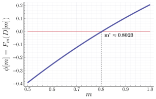
Figure 1. The function $\phi[m]$ for the example matrix (22).

Let us apply Newton’s method to compute $m^{\star}$, using the costless derivative formula in Theorem 4.2. The results are shown in Table 1, which show quadratic convergence.

$k$	$m$	$\phi[m]$	$\phi^{\prime}[m]$
$0$	$0.9$	$\ \ \,0.106308075414147$	$1.041560098368530$
$1$	$0.797933805662616$	$-0.005021877535631$	$1.140880961822965$
$2$	$0.802335559836519$	$-9.673874699522855\cdot 10^{-6}$	$1.136487060632446$
$3$	$0.{\bf 8023440719}21729$	$-3.612360410798487\cdot 10^{-11}$	$1.136478572827426$

Table 1. Example 22: quadratic convergence of Newton’s method.

5. A combinatorial relaxation

The numerical integration of (9) is certainly a demanding step in terms of CPU time. However, when slightly modifying the value $m$ (or considering a smooth function $A(t)$), in order to solve (9) for the new data, we propose an alternative strategy to the reintegration of (9), which is based on Theorem 3.1.

5.1. On the necessary condition (16) of Theorem 3.1

Theorem 3.1 provides an analytic condition to identify intermediate entries. Equation (16) is a codimension-$1$ condition. It means that for having entries of the extremizer $D[m]$ assuming intermediate values, either the $i$-th component of the eigenvector $x$ associated to the rightmost eigenvalue of $\mathrm{Sym}\left(D[m]A\right)$, or the $i$-th component of the vector $z=Ax$ have to vanish.

In the $2\times 2$ case it is direct to prove that extremizers are either

$${\rm diag}(1,m^{\star})\qquad\mbox{or}\qquad{\rm diag}(m^{\star},1),$$

and cannot assume intermediate values, as one expects. We omit the proof for sake of conciseness.

In the general $n$-dimensional case, assume that we know an extremizer $D[m]$, whose diagonal entries only assume the extremal values $m$ and $1$ and that the eigenvector $x$ of $\mathrm{Sym}(D[m]A)$ and the vector $z=Ax$ have entries suitably bounded away from zero. If we slightly perturb $m$ (or even the matrix $A$), then by continuity arguments we expect generically that the new extremizer has the same entry-pattern of $D[m]$, which means that the new vectors $\widetilde{x}$ and $\widetilde{z}$ remain close to $x$ and $z$ and thus have still non-zero entries. This remains true also for moderate changes of $m$. As an example, for the matrix (22) we get, using the proposed inner-outer scheme:

$$\left(x,x^{\star}\right)=\left(\begin{array}[]{rr}0.3836&0.3595\\ 0.6158&0.6664\\ 0.6882&0.6532\end{array}\right)\qquad\mbox{and}\qquad\left(z,z^{\star}\right)=\left(\begin{array}[]{rr}1.2251&1.2537\\ -1.5427&-1.7055\\ 0.3984&0.7059\\ \end{array}\right),$$

where $x$ indicates the rightmost eigenvector of $\mathrm{Sym}(A)$ and $z=Ax$, $x^{\star}$ the rightmost eigenvector of $\mathrm{Sym}(D_{m^{\star}}A)$ and $z^{\star}=Ax^{\star}$. This illustrates the slight change between the above starting vectors and those in the extremizer.

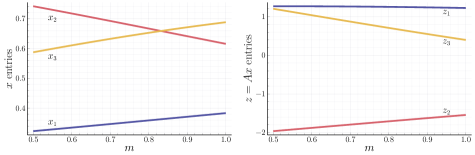
Figure 2. The behavior of the $3$ entries of $x$ (left) and $z=Ax$ (right) for extremizers for problem (22) as a function of $m$.

The plot (as a function of $m\in[m^{\star},1]$) of the entries of $x$ and of $z$ is shown in Figure 2.

Remark 5.1.

Extremizers in general are not unique. Consider for example the following matrix $A$ and $m=0.2$

$$A=\left(\begin{array}[]{ccc}-3&1&{3}/{2}\\ -1&-1&3\\ -1&-3&0\\ \end{array}\right),\qquad\mathrm{Sym}(A)=\left(\begin{array}[]{ccc}-3&0&{1}/{4}\\ 0&-1&0\\ {1}/{4}&0&0\\ \end{array}\right).$$

Then $D_{1}={\rm diag}\left(m,m,1\right)$, $D_{2}={\rm diag}\left(1,1,m\right)$ and $D_{3}={\rm diag}\left(m,1,m\right)$ are local extremizers, with $F_{m}(D_{1})=-1.1427$, $F_{m}(D_{2})=-0.8764$, $F_{m}(D_{3})=-0.8237$, so that $D_{1}$ is the global minimizer. Instead for the matrix $A$ in (22) with $m=0.8$ the extremizer $D={\rm diag}\left(1,m,1\right)$ turns out to be unique.

5.2. A greedy combinatorial algorithm

An algorithm to check possible extremizers only assuming extremal values is the following. Compute all possible diagonal matrices with combinatorial structure (which are $2^{n}$) and compute the gradient $G$ for each of them. Looking at the sign of the vector $G$ we can assert whether a certain matrix $D$ is a local extremizer.

Remark 5.2 (Efficient combinatorics).

The combinatorial algorithm is very expensive when $n$ increases. However, starting from the knowledge of an extremizer $D[m]$, the problem of minimizing $F_{m^{\prime}}$ for $m^{\prime}$ close to $m$, might be efficiently tackled by maintaining as an initial guess the extremizer $D[m]$, just replacing its entries equal to $m$ with the value $m^{\prime}$, and then checking the sign of the gradient. Similarly one could tackle the problem where the matrix $A$ instead of $m$ is slightly changed, as we will see in the next section. This would allow to avoid the numerical integration of the system of ODEs to minimize $F_{m^{\prime}}$ and is somehow reminiscent of an approach based on interior point methods as opposed to simplex methods in linear programming problems.

For example (22), this gives only the detected matrix (for all $m\leq m^{\star}$)

$$D[m]=\left(\begin{array}[]{rrr}1&0&0\\ 0&m&0\\ 0&0&1\end{array}\right).$$

For example, still considering Example (22), for the starting non-optimal diagonal matrix

$$D={\rm diag}\left(m,m,1\right),$$

with $m=0.9$, we get $\lambda=-0.1523$ and

$$G={\rm diag}\left(\mathbf{0.0700},-0.1602,0.0580\right),$$

which indicates that the optimality condition for the first entry is violated. Changing the value of the first entry to the opposite extremal value and modifying to

(23) $$\hat{D}[m]={\rm diag}\left(1,m,1\right),$$

allows us to find the optimal solution for the problem. At this point, it is sufficient to tune $m$ through the scalar equation

$$\mbox{find}\ m\ :\>\lambda_{\max}\left(\mathrm{Sym}(\hat{D}[m]A)\right)=0,$$

where $\hat{D}[m]$ has the structure in (23). to obtain the optimal value $m^{\star}\approx 0.8023$.

6. Time-dependent case: problems (P1) and (P2)

We are now interested to consider the more general time-varying problem setting where $A=A(t)$, for which we assume

$$\mu_{2}\left(A(t)\right)<0.$$

The problem now would be that of computing the function of $t$

(24) $$m^{\star}(t)=\operatorname*{argmin}\limits_{m\in[0,1]}\,\{m\ :\ \mu_{2}\left(DA(t)\right)\leq 0\quad\mbox{for all matrices $D\in\Omega_{m}$}\}.$$

We denote by $D[m](t)$ an associated extremizer, that is such that $\mu_{2}\left(D[m](t)A(t)\right)=0$, and by $m^{\star}(t)$ its smallest entry. To a given diagonal matrix $D\in\Omega_{m}$, we associate the structured matrix

$$S(D)=\{I_{1},I_{2},I_{3}\},$$

with

$$I_{1} = \{i\in\{1,\ldots,n\}:D_{ii}=1\},$$

(25) $$I_{2} = \{i\in\{1,\ldots,n\}:D_{ii}=m\},$$

$$I_{3} = \{i\in\{1,\ldots,n\}:D_{ii}=\beta_{i}\in(m,1)\}.$$

By continuity arguments, we have generically that the structure of $S(D[m](t))$ is piecewise constant along $[0,T]$, that means that indexes of the entries equal to $1$ and to $m(t)$, as well as those assuming intermediate values, remain so within certain intervals.

Let us consider the symmetric part of $D[m](t)A(t)$. Applying Lemma 3.1 to the rightmost eigenvalue of $\mathrm{Sym}(D[m](t)A(t))$, under smoothness assumptions we obtain (where time dependence is omitted for conciseness):

$$0\equiv\frac{d}{dt}\lambda=\dot{\lambda} = \frac{1}{2}x^{\top}\left(\dot{D}A+A^{\top}\dot{D}+D\dot{A}+\dot{A}^{\top}D\right)x$$

$$= \frac{1}{2}x^{\top}\left(\dot{D}A+A^{\top}\dot{D}\right)x+\gamma=x^{\top}\dot{D}z+\gamma,$$

with $z=Ax$ and

$$\gamma=x^{\top}\left(D\dot{A}+\dot{A}^{\top}D\right)x.$$

Then we have (exploiting Theorem 3.1)

$$\sum\limits_{i=1}^{n}x_{i}\dot{D}_{ii}z_{i}=\sum\limits_{i\in I_{2}}x_{i}\dot{D}_{ii}z_{i}=\left(\sum\limits_{i\in I_{2}}x_{i}z_{i}\right)\dot{m}^{\star}(t).$$

Consequently, we obtain the following scalar ODE for $m^{\star}(t)$,

(26) $$\dot{m}^{\star}(t)=-\frac{\gamma(t)}{\zeta(t)},\qquad\zeta(t)=\sum\limits_{i\in I_{2}}x_{i}(t)z_{i}(t).$$

This shows that from the sign of the r.h.s. of (26) we obtain the growth/decrease of $m^{\star}(t)$. The resulting algorithm for the time-varying case is discussed in the next subsection.

6.1. Algorithm for the time varying problem

On a uniform time grid $\{t_{k}\}_{k\geq 0}$ ($t_{k+1}=t_{k}+\Delta t$), given an extremizer $D(t_{k})$ with minimal entry $m^{\star}(t_{k})=m^{\star}_{k}$, we first approximate $m^{\star}(t_{k+1})$ by an Euler step (where we denote as $A^{(k)}=A(t_{k})$ and $\dot{A}^{(k)}=\dot{A}(t_{k})$):

$$m_{k+1}=m^{\star}_{k}-\Delta t\frac{\gamma_{k}}{\zeta_{k}},$$

with

$$\gamma_{k}=(x^{(k)})^{\top}\left(D^{(k)}\dot{A}^{(k)}+(\dot{A}^{(k)})^{\top}D^{(k)}\right)x^{(k)},\qquad\zeta_{k}=\sum\limits_{i\in I_{2}}x^{(k)}_{i}(t)z^{(k)}_{i}(t),$$

with $x^{(k)}$ eigenvector of $\mathrm{Sym}\left(D^{(k)}A^{(k)}\right)$ associated to the rightmost eigenvalue and $z^{(k)}=Ax^{(k)}$. Next, we update $D(t_{k+1})$ by setting its minimal entries as $m_{k+1}$ and compute $x^{(k+1)}$, i.e. the eigenvector of $\mathrm{Sym}\left(D^{(k+1)}A(t_{k+1})\right)$ associated to its rightmost eigenvalue, and set $z^{(k+1)}=Ax^{(k+1)}$. Then, in order to obtain a more accurate approximation of $m^{\star}_{k+1}$, we apply a single Newton step, as described in Section 4.3. Finally we verify that the resultant matrix $D^{(k+1)}=D[m^{\star}_{k+1}]$ is an extremizer by checking (see (25)

(27) $$x^{(k+1)}_{i}z^{(k+1)}_{i}>0\quad\mbox{for}\ i\in I_{1}\qquad\mbox{and}\qquad x^{(k+1)}_{i}z^{(k+1)}_{i}<0\quad\mbox{for}\ i\in I_{2}.$$

If, for at least one index $i$, one of the previous conditions (27) is violated, then an optimizer with a new structure is searched by running the whole Algorithm described in Section 4 for the matrix $A=A(t_{k+1})$.

6.2. Illustrative examples

Consider next the matrix

(28) $$A(t)=\left(\begin{array}[]{rr}-2-\sin(t)&\cos(t)\\ 2&-2-\cos(t)\end{array}\right),\qquad t\in[0,T],\ T=\pi,$$

which for $t=0$ coincides to Example (4.5). Figure 3(a) illustrates the behavior of $m^{\star}(t)$.

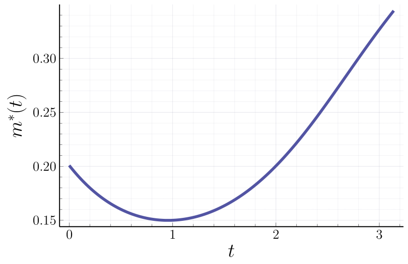
(a) $A(t)$ as in example (28).

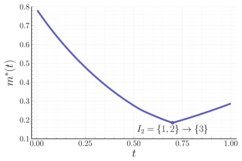
(b) $A(t)$ as in example (29).

Figure 3. Behaviour of $m^{\star}$ as a function of $t$, for two different matrix-valued functions $A(t)$.

Next, consider the matrix

(29) $$A(t)=\left(\begin{array}[]{ccc}-t-1&1&\frac{t}{2}+\frac{1}{2}\\ -1&t-3&t+1\\ 3-2t&1-2t&2t-4\\ \end{array}\right),\qquad t\in[0,T],\ T=1.$$

Figure 3(b) shows the sudden change of extremizer at $t\approx 0.7$. The set $I_{2}=\{1,2\}$ switches to $I_{2}=\{3\}$, when $t$ crosses the discontinuity point for $(m^{\star})^{\prime}(t)$.

6.3. Remarks

Applying the proposed method we obtain an accurate approximation of the extremizers $D[m](t)$ for the considered problem (24) for $t=t_{k},\ k=0,1,\ldots$ To have a uniform choice which guarantees contractivity we have to choose

$$m^{\star}=\max\limits_{k}\,m^{\star}_{k},$$

which might be too restrictive. Another possibility would be that of changing the slope $m=m(t)$ in the function $\sigma(t)$. Finally, relaxing the bound

$$\lambda_{\max}\left(\mathrm{Sym}\left(D[m](t)A(t)\right)\right)\leq 0\qquad\mbox{to}\qquad\lambda_{\max}\left(\mathrm{Sym}\left(D[m](t)A(t)\right)\right)\leq\alpha$$

for some moderate $\alpha>0$, would allow maintaining control on the growth of the solution (the constant $C$ in (3) would be $C\leq\mathrm{e}^{\alpha T}$), without restricting the range of $\sigma^{\prime}$.

6.4. A different outlook. Problem (P2): stability bound for fixed $m$

Assume that $m$ is fixed and we want to compute a bound for the growth of the error in the solution of Problem (P2), that is to get a worst-case estimate of the type (3). We write the solution to the differential equation ${\displaystyle{\dot{u}}=D(t)A(t)u}$, $u(t_{0})=u_{0}$ (with $D(t)$ unknown a priori), as

$$u(t)=\Phi(t,t_{0})u_{0}.$$

By Grönwall Lemma, it can be shown that a bound for the norm of the state transition matrix ${\displaystyle\Phi(t,t_{0})}$ is given by

$$\|\Phi(t,t_{0})\|\leq\exp\left(\int\limits_{t_{0}}^{t}\mu_{2}\left(D(s)A(s)\right)ds\right),$$

for all $t\geq t_{0}$. This means that if we compute the worst case quantity $\mu_{2}(s)=\mu_{2}(D(s)A(s))$ for $D(s)\in\Omega_{m}$, by applying a quadrature formula we get an upper bound for the constant $C$, that is

(30) $$C\leq\exp\left(\int\limits_{0}^{T}\mu_{2}\left(\widetilde{D}(s)A(s)\right)ds\right)\approx\exp\left(Q\left[\mu_{2}\left(\widetilde{D}(s)A(s)\right)\right]\right):=\widetilde{C},$$

with $\widetilde{D}(t)=\operatorname*{argmax}\limits_{D\in\Omega_{m}}\mu_{2}\left(DA(t)\right)$ and $Q[\cdot]$ a suitable quadrature formula, e.g. the trapezoidal rule.

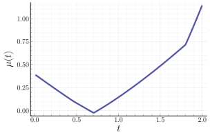
Figure 4. The behavior (for fixed $m$) of $\mu_{2}(t)$ (see (31)) for the matrix-valued function (29) as a function of $t$.

Figure 4 illustrates the behavior of

(31) $$\mu_{2}(t):=\mu_{2}\left(\widetilde{D}(t)A(t)\right)$$

for the matrix-valued function $A(t)$ of example (29), where for the quadrature we have used trapezoidal rule.

Remark 6.1.

It is not guaranteed that there exists a trajectory $u(t)$ of the dynamical system (2) to which corresponds the critical matrix sequence $\widetilde{D}(t)$. However, if such a trajectory exists, then the bound (30) is sharp.

6.5. Illustrative example

Let us consider the Cauchy problem (2) with $T=2$ and the example matrix (29). Note that, for $m=0.5$, the problem is strictly contractive in the spectral norm. We compute the upper bound (30) for several values of $m$. The results are illustrated in Table 2.

$m$	$\min\limits_{t}\mu_{2}(t)$	$Q[\mu_{2}(t)]$	$\widetilde{C}$
$0.01$	$0.2890$	$1.2467$	$3.4787$
$0.05$	$0.2202$	$1.1170$	$3.0556$
$0.1$	$0.1379$	$0.9605$	$2.6129$
$0.2$	$-0.0216$	$0.6610$	$1.9368$
$0.5$	$-0.4076$	$-0.1414$	$0.8681$

Table 2. The upper bound $\widetilde{C}$ for Example (29).

7. An application: a neural network for digits classification

To conclude, we apply the theory developed in the previous sections to increase the robustness of a neural ODE image classifier. To this end, we consider MNIST handwritten digits dataset [8] perturbed via the Fast Gradient Sign Method (FGSM) adversarial attack [9].

Let us recall that MNIST consists of 70000 $28\times 28$ grayscale images (60000 training images and 10000 testing images), that is vectors of length 784 after vectorization. We consider a neural network made up of the following blocks:

1. a downsampling affine layer that reduces the dimension of the input from 784 to 64, i.e. a simple transformation of the kind $y=A_{1}x+b_{1}$, where $x\in\mathbb{R}^{784}$ is the input, $y\in\mathbb{R}^{64}$ is the output, and $A_{1}\in\mathbb{R}^{64,784}$ and $b_{1}\in\mathbb{R}^{64}$ are the parameters;

2. a neural ODE block that models the feature propagation,

   $$\begin{cases}\dot{x}(t)=\sigma\left(Ax(t)+b\right),\qquad t\in[0,1],\\ x(0)=y,\end{cases}$$

   whose initial value is the output of the previous layer, where $x(t):[0,1]\to\mathbb{R}^{64}$ is the feature vector evolution function, $A\in\mathbb{R}^{64,64}$ and $b\in\mathbb{R}^{64}$ are the parameters, and $\sigma$ is a custom activation function, defined as

   $$\sigma(x)=\begin{cases}x,\qquad&\mbox{if }x\geq 0,\\ \tanh{x},\qquad&\mbox{if }-\bar{x}\leq x<0,\\ \alpha x,\qquad&\mbox{otherwise},\end{cases}$$

   where $\bar{x}>0$ is such that $\tanh^{\prime}{(\pm\bar{x})}=\alpha=0.1$ (see Figure 5);

   

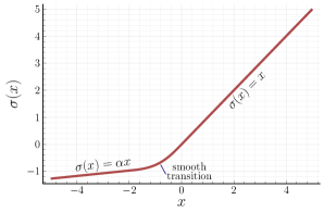
   Figure 5. Custom activation function: a smoothed Leaky Rectified Linear Unit (LeakyReLU) with minimal slope $\alpha=0.1$.

3. a final classification layer that reduces the dimension of the input from 64 to 10, followed by the softmax activation function

   $$x_{out}=\mbox{softmax}\left(A_{2}x(1)+b_{2}\right),$$

   where $x(1)\in\mathbb{R}^{64}$ is the output of the neural ODE block, $A_{2}\in\mathbb{R}^{10,64}$ and $b_{2}\in\mathbb{R}^{10}$ are the parameters, and $x_{out}$ is the output vector whose component $i$ is the probability that the input $x$ belongs to the class $i$. Recall that softmax is a vector-valued function that maps the vector $x$ into the vector $\mbox{softmax}(x)=e^{x}\|e^{x}\|_{1}^{-1}$, where exponentiation is done entrywise.

We require the neural ODE block to be contractive, so that small perturbations added to the input, such as adversarial attacks, are not amplified.

Making use of the proposed algorithm, we compute the smallest value $m^{\star}$ that the entries of the diagonal matrix $D$ can assume, such that

(32) $$\sup\left\{\mu_{2}(DA),\ \forall D\in\mathbb{D}^{64,64}\mbox{ such that }D_{ii}\in[m^{\star},1]\right\}=0,$$

If the value $m^{\star}$ computed by the algorithm in Section 4.3 is larger than $\alpha$, we set $\delta>0$ a small positive constant and replace the matrix $A$ by the shifted matrix

$$\widehat{A}=A-\ell\delta I,$$

where $\ell$ is the smallest positive integer such that (32) holds for $\widehat{A}$ in place of $A$.

Note that shifting the matrix $A$, and thus its entire spectrum, to get $m^{\star}$ below the specified threshold $\alpha$, is a greedy algorithm that allows us to obtain (32). Other strategies may be used here, including computing the nearest matrix in some suitable metric, such that $m^{\star}\leq\alpha$ to $A$.

We add these additional steps to the standard training methodology via adjoint method [7] after parameter initialization and after each step of gradient descent. Then, we train a first copy of the above-mentioned neural network according to standard training, and we train a second copy of the same neural network employing the proposed modification to the standard training. The networks are trained for 70 epochs. We eventually compare in Table 3 the test accuracy (the percentage of correctly classified testing images) of the two models (the standard one and the stabilized one, obtained imposing contractivity) as a function of $\epsilon>0$, the size in the $L^{\infty}$-norm of the FGSM perturbation to each testing image, i.e. if $x_{i}$ is a testing image, $x_{i}+\varepsilon\delta_{i}$ is the perturbed testing image, with $\delta_{i}$ the FGSM attack to $x_{i}$, $\|\delta_{i}\|_{\infty}=1$. Incorporating the tuning and shifting strategy proposed here, we observe a clear improvement in robustness against the FGSM attack.

$\varepsilon$	0	0.01	0.02	0.03	0.04	0.05	0.06
Standard NN	97.29%	94.49%	89.07%	77.73%	61.95%	46.61%	34.14%
Proposed NN	97.27%	95.30%	92.08%	86.88%	77.81%	63.56%	48.86%

Table 3. Comparison of test accuracy as a function of $\varepsilon$.

8. Conclusions and future works

In this article we have proposed a novel methodology to solve numerically a class of eigenvalue optimization problems arising when analyzing contractivity of neural ODEs. Solving such problems is essential in order to make a neural ODE stable (contractive) with respect to perturbations of initial data, and thus preventing the output of the neural ODE to be sensitive to small input perturbations, such those induced by adversarial attacks.

The proposed method consists of a two-level nested algorithm, consisting of an inner iteration for the solution of an inner eigenvalue optimization problem by a gradient system approach, and in an outer iteration tuning a parameter of the problem until a certain scalar equation is verified.

The proposed algorithm appears to be fast and its behaviour has been analyzed through several numerical examples, showing its effectiveness and reliability. A real application of a neural ODE to digits classification shows how this algorithm can be easily embedded in the contractive training of a neural ODE, making it robust and stable against adversarial attacks.

Acknowledgments

N.G. acknowledges that his research was supported by funds from the Italian MUR (Ministero dell’Università e della Ricerca) within the PRIN 2022 Project “Advanced numerical methods for time dependent parametric partial differential equations with applications” and the Pro3 joint project entitled “Calcolo scientifico per le scienze naturali, sociali e applicazioni: sviluppo metodologico e tecnologico”. N.G. and F.T. acknowledge support from MUR-PRO3 grant STANDS and PRIN-PNRR grant FIN4GEO.

The authors are members of the INdAM-GNCS (Gruppo Nazionale di Calcolo Scientifico).

References

- [1] R. Caldelli, F. Carrara, and F. Falchi, Tuning Neural ODE Networks to Increase Adversarial Robustness in Image Forensics, 2022 IEEE International Conference on Image Processing (ICIP), IEEE, 2022, pp. 1496–1500.
- [2] F. Carrara, R. Caldelli, F. Falchi, and G. Amato, On the Robustness to Adversarial Examples of Neural ODE Image Classifiers, 2019 IEEE International Workshop on Information Forensics and Security (WIFS), IEEE, 2019, pp. 1–6.
- [3] by same author, Defending Neural ODE Image Classifiers from Adversarial Attacks with Tolerance Randomization, International Conference on Pattern Recognition, Springer, 2021, pp. 425–438.
- [4] by same author, Improving the Adversarial Robustness of Neural ODE Image Classifiers by Tuning the Tolerance Parameter, Information 13 (2022), no. 12, 555.
- [5] E. Celledoni, M. J. Ehrhardt, C. Etmann, R. I. Mclachlan, B. Owren, C.-B. Schonlieb, and F. Sherry, Structure-Preserving Deep Learning, European J. Appl. Math. 32 (2021), no. 5, 888–936. MR 4308177
- [6] B. Chang, L. Meng, E. Haber, L. Ruthotto, D. Begert, and E. Holtham, Reversible Architectures for Arbitrarily Deep Residual Neural Networks, Proceedings of the AAAI Conference on Artificial Intelligence, vol. 32, 2018.
- [7] R. T. Q. Chen, Y. Rubanova, J. Bettencourt, and D. K. Duvenaud, Neural Ordinary Differential Equations, Advances in Neural Information Processing Systems 31 (2018).
- [8] L. Deng, The MNIST Database of Handwritten Digit Images for Machine Learning Research, IEEE Signal Processing Magazine 29 (2012), no. 6, 141–142.
- [9] I. J. Goodfellow, J. Shlens, and C. Szegedy, Explaining and Harnessing Adversarial Examples, arXiv preprint arXiv:1412.6572 (2014).
- [10] E. Haber and L. Ruthotto, Stable Architectures for Deep Neural Networks, Inverse Problems 34 (2018), no. 1, 014004, 22. MR 3742361
- [11] K. He, X. Zhang, S. Ren, and J. Sun, Deep Residual Learning for Image Recognition, Proceedings of the IEEE Conference on Computer Vision and Pattern Recognition, 2016, pp. 770–778.
- [12] Y. Huang, Y. Yu, H. Zhang, Y. Ma, and Y. Yao, Adversarial Robustness of Stabilized Neural ODE Might Be From Obfuscated Gradients, Mathematical and Scientific Machine Learning, PMLR, 2022, pp. 497–515.
- [13] Q. Kang, Y. Song, Q. Ding, and W.P. Tay, Stable Neural ODE with Lyapunov-Stable Equilibrium Points for Defending against Adversarial Attacks, Advances in Neural Information Processing Systems 34 (2021), 14925–14937.
- [14] T. Kato, Perturbation Theory for Linear Operators, vol. 132, Springer Science & Business Media, 2013.
- [15] M. Li, L. He, and Z. Lin, Implicit Euler Skip Connections: Enhancing Adversarial Robustness via Numerical Stability, International Conference on Machine Learning, PMLR, 2020, pp. 5874–5883.
- [16] X. Li, Z. Xin, and W. Liu, Defending Against Adversarial Attacks via Neural Dynamic System, Advances in Neural Information Processing Systems 35 (2022), 6372–6383.
- [17] Gustaf Söderlind, The logarithmic norm. History and modern theory, BIT 46 (2006), no. 3, 631–652.
- [18] H. Yan, J. Du, V.Y.F. Tan, and J. Feng, On Robustness of Neural Ordinary Differential Equations, arXiv preprint arXiv:1910.05513 (2019).