Gravitational Wave Signal Extraction Against Non-Stationary Instrumental Noises with Deep Neural Network
Abstract
Sapce-borne gravitational wave antennas, such as LISA and LISA-like mission (Taiji and Tianqin), will offer novel perspectives for exploring our Universe while introduce new challenges, especially in data analysis. Aside from the known challenges like high parameter space dimension, superposition of large number of signals and etc., gravitational wave detections in space would be more seriously affected by anomalies or non-stationarities in the science measurements. Considering the three types of foreseeable non-stationarities including data gaps, transients (glitches), and time-varying noise auto-correlations, which may come from routine maintenance or unexpected disturbances during science operations, we developed a deep learning model for accurate signal extractions confronted with such anomalous scenarios. Our model exhibits the same performance as the current state-of-the-art models do for the ideal and anomaly free scenario, while shows remarkable adaptability in extractions of coalescing massive black hole binary signal against all three types of non-stationarities and even their mixtures. This also provide new explorations into the robustness studies of deep learning models for data processing in space-borne gravitational wave missions.
I INTRODUCTION
Since the first landmark event GW150914 captured by Adv-LIGO [1], today nearly a hundred Gravitational Wave (GW) signals from mergers of stellar mass compact binaries had been observed by the LIGO-VRIGO collaboration, which lead to numerous accomplishments in astrophysics and fundamental physics [2, 3, 4, 5, 6, 7, 8, 9, 10, 11, 12, 13, 14]. However, limited by seismic noises, ground-based GW detectors are typically sensitive to signals at frequencies higher than 10 Hz [15, 16, 17]. To enclose the exciting sources of larger and heavier astrophysical systems, one needs to explore the low frequency band of the GW spectrum with detectors of much longer baselines. The first generation space-borne antennas, including LISA (Laser Interferometer Space Antenna) [18, 19] and the LISA-like missions Taiji [20, 21] and Tianqin [22], would be launched in the 2030s and cover the mHz band. Offering novel perspectives for exploring the Universe, such space-borne antennas will also introduce new challenges [19], especially in data analysis [23, 24, 25].
Space antennas are supposed to response to a large amount of superimposed GW signals, including coalescing (super) Massive Black Hole Binaries (MBHB), extreme-mass-ratio-inspirals, galactic compact binaries, evolving topological defects, primordial GW background, and also un-modeled sources. To gain considerable Signal-to-Noise Ratios (SNR) against the overwhelming noises, one generally needs to accumulate data for rather long periods, even for years, which largely increases the computational costs in data processing. The high parameter space dimension of each type of sources adds more complexities and challenges. Many works have been done to address those issues [26, 27, 28]. As lessons learned from the LIGO-VIRGO observatories [29] and precedent missions like GRACE/GFO [30], LISA PathFinder (LPF) [31] and also Taiji-1 [32], new issues in data analysis for space-borne GW detections begin to draw more attentions [33, 34, 35, 36, 25]. As mentioned, to precisely measure the related parameters and infer the physical properties of the sources, continues measurements without disruptions in the data are normally demanded, which however imposes hard challenges on the long-term stability and robustness of both the payloads and satellite platforms. GW detection in space would be more seriously affected by anomalies or non-stationarities in the science measurements, including instrument transients or noise bursts, data gaps, slowly varying noise auto-correlations, trends and etc, as the detailed knowledge of instrumental noises is crucial to GW signals extraction and parameter estimations. According to the designs of the LISA and Taiji missions, the foreseeable anomalies or non-stationarities in science measurements may come from the routine maintenance of the satellites or the onboard payloads and unexpected environment disturbances or instrumental anomalies, which will be the main subjects of this work. Cyclostationary properties also exist mainly due to the orbital modulations of the stochastic GW foreground from compact binaries, which are not within the scope of this work and will be left for future studies.
Routine maintenance, such as antenna re-orientations, payloads calibrations and etc., could cause important and even continuous disturbances of satellite platforms and affect heavily the performances of the key payloads, therefore result into varying noise auto-correlations and even data loss or gaps. For example, the scheduled re-orientations of the transmission antennas would lead to data gaps about 3.5 hours per week or 7 hours every two-weeks [33, 37]. In addition, unforeseen anomalies or failures due to hardware problems would take place and produce random unscheduled data gaps. Based on the experiences from LPF [38, 34, 24, 36], GRACE/GFO [39, 40] and also Taiji-1 [41], instrumental transients may also contaminate the science data, such as the acceleration glitches in gravitational reference sensor (GRS) systems, phase jumps in interferometers, and etc. Early studies on data processing algorithms against such possible anomalies can be found in [33, 35, 36]. Recently, Dey et al. [23] have used Bayesian analysis techniques to assess the impact of data gaps and concluded that the effects of unscheduled gaps were often more significant, and Spadaro et al. [42] used a joint parameter estimation approach to evaluate the influences of GRS glitches demonstrating that it is possible to accurately identify glitches in the absence of overlapping GW signals. These studies treated the above non-stationarities independently, and, for instrumental transients, prior knowledge of transient models are required. In this work, given the potentials and capacities of deep neural networks, we seek to develop an anomaly-model-independent signal extraction method for space GW antennas that can thoroughly treat and overcome the impacts of the above three types of data non-stationarities or anomalies.
Deep learning methods have already achieved considerable success in data processing of GW detections [43, 44, 45, 46, 47, 48, 49, 50, 51, 52, 53, 54]. Compared to traditional algorithms, such as matched filtering [55, 56, 57], which generally require a vast template bank and thus consume substantial computational resources, deep learning methods are well known for their fast processing speed and excellent generalization ability, making it possible to achieve rapid and anomaly-model-independent signal extraction. For GW detection in space, Conv-TasNet [54] has demonstrated its performance in various scenarios, claiming an extraction speed improvement of up to times compared to traditional methods, however, robustness tests under anomalous conditions are overlooked. In this work, focusing on the three types of possible non-stationarities for LISA or LISA-like missions, including gaps, transients (glitches), and time varying noise auto-correlations, we developed a deep learning model for accurate extractions of coalescing MBHB signals confronted with such anomalous scenarios. This also provide new explorations into the robustness studies of deep learning models for data processing in space-borne GW missions. Our model exhibits the same performance as the Conv-TasNet model [54] does for the ideal and anomaly free scenario, while shows remarkable adaptability in signal extractions against all three types of non-stationarities and even their mixtures.
II Dense-LSTM model
Autoencoders, commonly employed as denoising architectures, are extensively applied in fields like image denoising [58, 59, 60, 61], signal extractions [62, 63, 64, 65], and speech enhancements, et al. [66, 67, 68, 69]. Autoencoder models include an encoder and a decoder. The encoder is designed to extract feature mappings from the input data, while the decoder is to generate reconstructed data from these mappings. For GW signal extractions in LIGO-VIRGO data analysis, the CNN-LSTM denoising autoencoder model has been used [70] and shown superior performance.
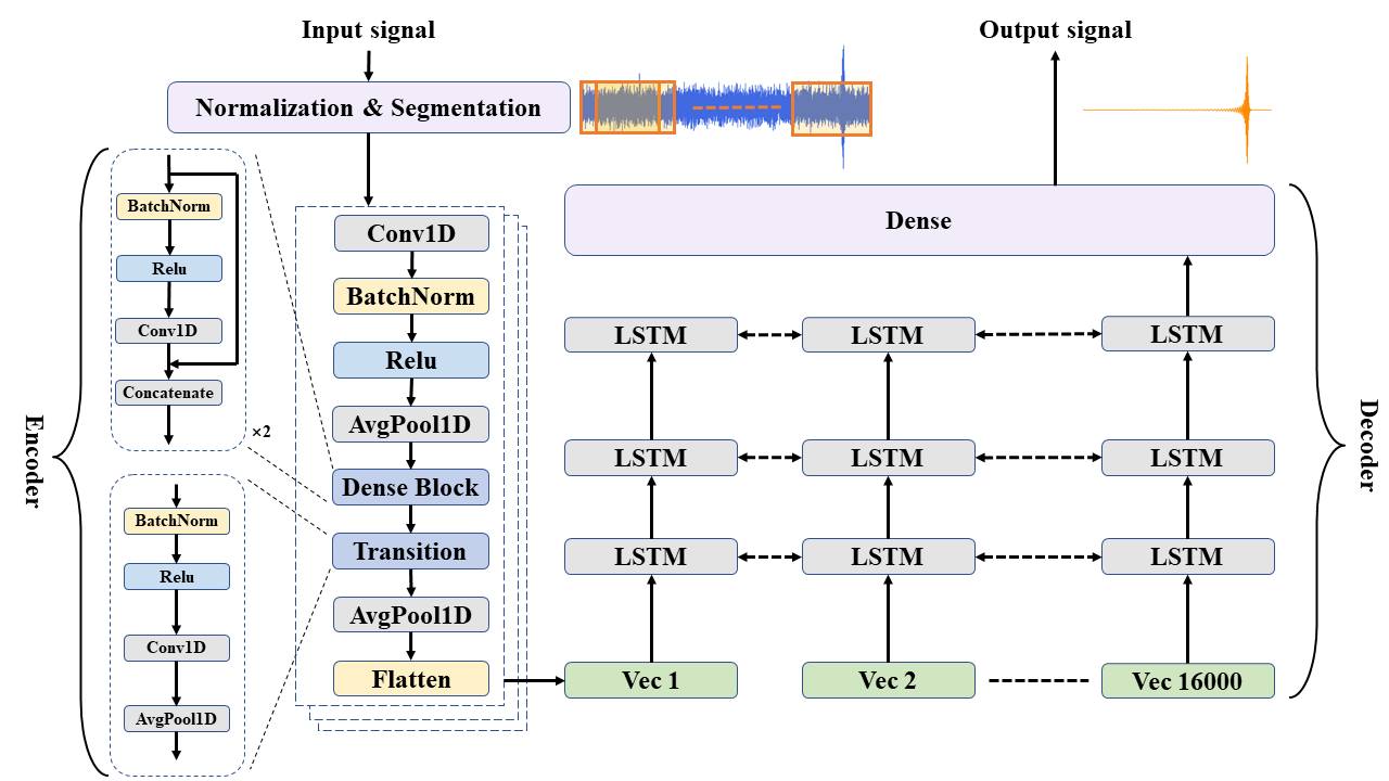
As discussed in Sec. I, the long periods and consequently the much more complicated data anomalies for science measurements of LISA and LISA-like missions have driven us to develop models capable of uncovering deeper mappings within the signals and thereby reducing the loss and alteration of the crucial information under significant anomalous conditions. Simple CNN architectures fall short in meeting these demands. In this work, we choose to use a deeper CNN network different from the CNN-LSTM denoising autoencoder suggested by Chatterjee et al. [70]. The DenseNet is chosen as the encoder for its advantage in reducing computational overhead while maintaining comparable accuracy compared with other deep CNN networks [71, 72, 73, 74] and at the same time ensuring faster feature extraction. More importantly, DenseNet thoroughly implements the concept of feature reuse, with each layer directly connected to all preceding layers. This enables the comprehensive utilization of low-complexity shallow features, facilitating the derivation of a smoother and more robust decision function. Such a design ensures considerable extraction capabilities even when confronted with data strongly contaminated by the possible non-stationarities or anomalies for space-borne GW detections. For the decoder, we retain the bidirectional LSTM network due to its superiority in capturing long-term dependencies within sequences.
The structure of our model is depicted in Fig 1. The input GW data for the model have a sampling frequency of 0.1Hz and a duration of 160,000 seconds, amounting to 16,000 data points. The detailed data preparations can be found in Sec III. All data are normalized between -1 and 1, followed by segmentation into 16,000 overlapping subsequences of length 4. Each subsequence is then fed into the decoder network for feature extraction. The feature vector of each subsequence is processed through three bidirectional LSTM layers for predicting the output of the subsequent time step. Finally, a complete waveform output is obtained through a dense layer.
III Data preparations
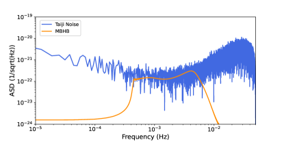
For LISA and LISA-like missions, laser frequency instability noise is dominant in the science measurements, and a post-processing technology called Time Delay Interferometry (TDI) [75, 76, 17] is employed to efficiently suppress such noise. Next important noises including clock noises, tilt-to-length noises and etc. could also be resolved within the TDI framework [77, 78], and the noise floor of the output data from certain TDI channel is in principle determined by combinations of GRS residual acceleration noises and optical readout noises . Following this, our data is generated through the first generation noise orthogonal TDI channels and , see [75] for details. The total noise Power Spectral Density (PSD) of the , channels are the combinations of the PSDs of the two noise components and , see Ref [79, 80, 81] for their specific combination forms, and according to the designs of LISA [19] and Taiji [82] we assume the nominal values
| (1) |
| (2) |
The transformed signals from incident GWs through the and channels reads
| (3) |
where is the transfer function combining antenna responses and TDI transformations, and is the polarized wave-train of the coalescing MBHB GW signal. The PyCBC package[83] and the waveform model SEOBNRv4 [84] are employed to generate the coalescing MBHB GW templates.
We established the parameter space for coalescing MBHBs as in Table 1, and employed a uniform grid to generate the diverse waveforms. Parameters such as times and phases at coalescence, sky locations, polarization angles, as well as inclinations are drawn from uniform distributions. The luminosity distances are used as a normalization factor to adjust the SNRs of signals.
| Parameter | Lower bound | Upper bound |
|---|---|---|
| 111Total mass of the system. | ||
| 222Mass ratio of the objects in the binary system. | 0.01 | 1 |
| 333Dimensionless spin parameter for the primary object. | -0.99 | 0.99 |
| 444Dimensionless spin parameter for the secondary object. | -0.99 | 0.99 |
We inject the signal with specific SNR
| (4) |
where represents the signal template through channel , the inner product is defined as,
| (5) |
here Hz and Hz. The tilde symbol represents the Fourier transform and the complex conjugation. We set the SNR level for the training dataset as 50, and generate 10,000 samples. All samples are subjected to whitening processing, and a Tukey window with is adopted. The overlap between the output signal from our model and a template waveform can be evaluated in terms of the overlap function
| (6) |
where and are the normalized ones, and and are the instantaneous time and phase corresponding to the maximum overlap between and .
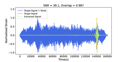
Following the same routine, we produce 2,000 test samples, see Fig 2 for illustration. In order to assess the model’s performance for signals extractions with different levels of SNRs, these samples were generated with SNRs ranging from 30 to 70.
IV Training strategy
For denoising autoencoders, the Mean Squared Error (MSE) is a prevalent loss function employed to quantify the discrepancy between the network’s predictions and the true values. However, given that the GW signals fed into the network have undergone normalization, the contributions to the overall MSE from the earlier stages of the coalescing signals are rather weak compared to those from the merger phases. This can hinder the model from achieving optimal refinements. To address this, the loss function defined in [70] is adopted which is the difference of the MSE and the fractal Tanimoto similarity coefficient [85] terms
| (7) |
the first term on the right hand side is the MSE term and the fractal Tanimoto similarity coefficient is defined as
| (8) |
The MSE is used for the optimizations of individual data points, while the fractal Tanimoto similarity coefficient is for the optimizations of the overall data. Tanimoto coefficient is commonly used to measure the similarity between two vectors, and the fractal coefficient, as an enhanced version, introduces a parameter to facilitate deeper levels of optimizations. This approach ensures that the extracted data achieves good amplitude and phase agreements with the template data on a global level.
Another worth-noting modification is that, unlike in the original work [70] where the weight is set to , we set equal to 1 in our approach. This is because, the long observation time in space borne GW detection will give rise to large number of data points that having amplitudes close to zero in the generated templates, the high weights, such as , of these data points will consequently prevent the network from converging. For the parameter , which is used to adjust the depth of optimization in similarity, is initially set to 0. As the training converges, grows gradually to facilitate deeper levels of optimization.
To summarize, at the beginning of the training, we set the learning rate to and to 0. As the model approaches convergence, we set and reduce the learning rate by a factor of 10. We have chosen the learning rate as , , and with corresponding taking values as 0, 5, and 10 for case studies, and trained for 200 epochs for each case.
V Results
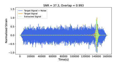
We first tested the extraction performance of our model for the ideal case without data non-stationarities or anomalies, see illustrations in Fig 3. More than 99% of the signals extracted by the model achieve an overlap 0.9 with the corresponding template, and each signal could be extracted in less than seconds. This demonstrates a similar performance of our model compared to the current state-of-the-art models [54]. In the followings, we conduct various tests of our model against the possible non-stationarities or anomalies known to the literature, including data gaps, time-varying noise auto-correlations, glitches, and even their mixtures. We expect that at least 80% of the signals extracted by the model should attain an overlap 0.9 with the template signals, which we will use as the criterion for assessing the limits of the model’s performance. The physical meanings of a more realistic criterion or threshold should come from more detailed studies on false positive, uncertainties in parameters estimations and so on, which will be left for future studies.
V.1 Data gaps
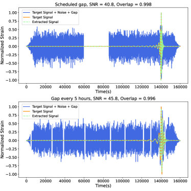
Following the discussions in [23], we use window functions to generate data gaps (see Ref [23] for the specific forms), which, as discussed in Sec. I can be classified into two types, that the scheduled prolonged gaps and unscheduled random but short gaps. For the scheduled gaps, we emulate an extreme situation, resulting into a data loss of 7 hours during the inspiral phases. For unscheduled gaps, we set each gap to cause 5 to 8 minutes of data loss, and progressively increase the frequency of occurrences of such randomly happened gaps to a threshold at which our model can hardly tolerate. Moreover, the unscheduled gaps are allowed to break out at any place of our data, while a prolonged data gap during the merger phase is ignored for obvious reason. Our extraction results are presented in Fig 4. Our model can proficiently extract the signals despite facing these two types of data gaps.
We delved further into the threshold performance of our model, as detailed in Fig 5. The model exhibits minimal accuracy loss in scenarios with scheduled gaps before mergers. When confronted with the random unscheduled gaps, the model’s results gradually worsen as the frequency of occurrences increases. As expected, signals with lower SNRs are more susceptible to data gaps. In Tab 2, we present more detailed results under different conditions. According to the predetermined criterion, our model can maintain robustness even when the frequency of unscheduled gaps reaches once per 5-hours.
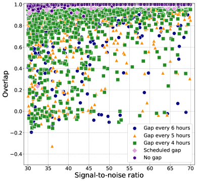
| Type of gap | Overlaps 0.9 |
|---|---|
| No gap | 99% |
| Scheduled gap | 99% |
| Gap every 6 hours | 86% |
| Gap every 5 hours | 83% |
| Gap every 4 hours | 77% |
V.2 Time-varying noise auto-correlations
We simulated non-stationary noises with time-varying auto-correlations or PSDs by altering the magnitudes of and of the two noise components, with the modified noise segment lasting for 80,000 seconds. In Fig 6, we present one of our extraction samples. The limits of our model’s performance against such non-stationary noise is investigated and shown in Fig 7. As expected, data with lower SNRs will be more significantly affected by time-varying noise PSDs, and the detailed results are presented in Tab 3. Our model can successfully extract the signal without being affected by such variations in total noise PSDs.
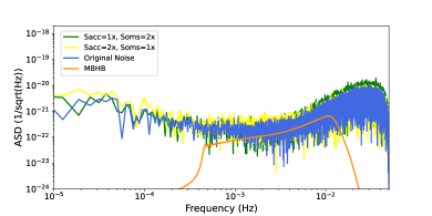
While, given the predefined criterion, one finds that noises originating from the optical metrology system has a more significant impact on the final outcomes. Further investigation shows that this is because that, increasing the optical readout noise (concentrated in the relatively high frequency band) will significantly reduce the SNR of coalescing MBHB signals due to the specific forms of the PSDs of the total noise and expected signal, see Fig 8 for illustrations. This, but not the variations in noise PSDs, will make it more difficult for the model to extract signals and produce the results shown Fig 7. and Tab 3.
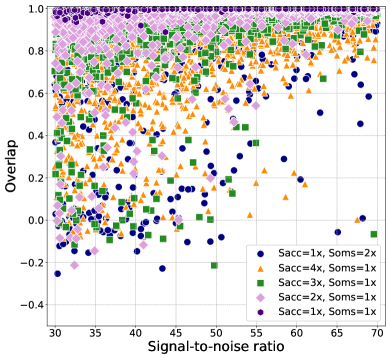
| Overlaps 0.9 | ||
|---|---|---|
| 1x | 1x | 99% |
| 1x | 2x | 92% |
| 1x | 3x | 81% |
| 1x | 4x | 54% |
| 2x | 1x | 77% |
V.3 Glitches
For instrumental transients, we consider the legacy model from LISA Pathfinder for GRS glitches as representatives [36]
| (9) |
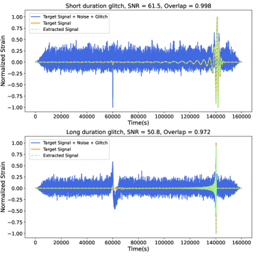
where is the time of glitch injection, is the impulse transferred by the glitch (i.e., the gain of test mass velocity caused by the glitch), are time scales, and denotes the Heaviside step function. Glitches are simulated and injected to one of the test mass interferometer measurement. The detailed transfer functions of glitches to the TDI outputs can be found in Ref. [35]. We considered two types of glitches according to Ref. [36], that the short-duration glitches lasting approximately 70 seconds and long-duration glitches for about 3 hours. To facilitate our evaluation, we have set the initial amplitude of both types of glitches to . Our model proficiently extracts the coalescing MBHB signals given such instrumental transients. Fig 9 shows an example of the model’s extraction result.
| Duration | Peak value(ms-2) | Overlaps 0.9 |
|---|---|---|
| None | None | 99% |
| Short | 99% | |
| Short | 99% | |
| Short | 95% | |
| Short | 72% | |
| Long | 99% | |
| Long | 71% |
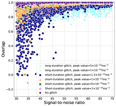
The limits of our model’s performance against glitches is shown in Fig 10. The results indicate that the performance deteriorates as the duration of the glitch increases, and detailed results are presented in Tab 4. Specifically, for short-duration glitches, the maximum tolerable magnitude of the glitch is about , while for long-duration glitches, the maximum tolerable magnitude is about .
V.4 Mixing three types of non-stationarities
| Data gaps | Non-stationary Gaussian noise | Glitches | Overlaps 0.9 | |||
|---|---|---|---|---|---|---|
| Scheduled gap | Unscheduled gap | Duration | Peak value (ms-2) | |||
| 1x | 3x | Short | 83% | |||
| 1x | 3x | Long | 81% | |||
| Gap every 10 hours | 1x | 2x | Short | 81% | ||
| Gap every 10 hours | 1x | 2x | Long | 81% | ||
At last but not least, we conducted tests by mixing three types of non-stationarities and have listed in Tab 5 the results achieved by our model under different conditions. When all these combine, our model still exhibits considerable extraction capability. When long-term scheduled gap exists, our model can tolerate with time-varying noise PSDs together with short-duration glitches of maximum peak value or long-duration glitches . When the occurrence frequency of unscheduled gaps reaches about once every 10 hours, our model can tolerate with relative weaker changes in noise (residual acceleration noise) PSDs combined with short-duration glitches of maximum peak value or long-duration glitches . These tests give typically the possible extreme cases in real science operations and measurements of space-borne GW antennas, and our model have shown high robustness and feasibility in typical signal extractions. It can be observed that high-frequency unscheduled gaps may have important impacts, which is predominantly due to substantial loss of spectral information and further compounded by additional anomalies that significantly obfuscate the model’s signal extraction capabilities. In future works, we will try to improve the model’s ability to tolerate these mixed situations in order to improve performance in more extreme situations, and we will focus on unscheduled gaps, improving the model’s tolerance for this situation and mitigating its impact on other anomalies.
VI Concluding remarks
In this work, we developed a deep learning model for accurate GW extractions against possible data anomalies or non-stationarities for space-borne GW antennas, such as LISA and LISA-like missions, which also provide robustness studies of deep learning models in data processing of space-borne GW missions. Our research focuses on the three types of non-stationarities, including gaps, glitches, and time varying noise auto-correlations. Compared with the current state-of-the-art models, our model exhibits the same performance for the ideal and anomaly free cases in signal extractions. While, confronted with the three types of non-stationarities and even their mixtures in some extreme cases, our model still shows considerable adaptability. It is worth noting that when all anomalies occur at the same time, the model’s tolerance for these anomalies would degrade compared with each stand-alone situation, and among these the unscheduled gap turns out to be a more important factors.
Deep learning has provided a method for the rapid detection of space-borne GW missions, and robustness research is key to ensuring that deep learning models are applicable in real detection scenarios. It is planned to process longer datasets in future works and to incorporate a greater variety of realistic simulation scenarios, including various levels of SNR and types of anomalies. Additionally, we will focus on unscheduled gaps, seeking new improvements to mitigate the substantial impact of such anomalies on model performance.
Acknowledgements.
This work is supported by the National Key Research and Development Program of China No. 2021YFC2201901, No. 2021YFC2201903, No. 2020YFC2200601 and No. 2020YFC2200901.References
- Abbott et al. [2016a] B. P. Abbott, R. Abbott, T. Abbott, M. Abernathy, F. Acernese, K. Ackley, C. Adams, T. Adams, P. Addesso, R. Adhikari, et al., Gw150914: The advanced ligo detectors in the era of first discoveries, Physical review letters 116, 131103 (2016a).
- Abbott et al. [2016b] B. P. Abbott, R. Abbott, T. Abbott, M. Abernathy, F. Acernese, K. Ackley, C. Adams, T. Adams, P. Addesso, R. Adhikari, et al., Observation of gravitational waves from a binary black hole merger, Physical review letters 116, 061102 (2016b).
- Abbott et al. [2016c] B. P. Abbott, R. Abbott, T. Abbott, M. Abernathy, F. Acernese, K. Ackley, C. Adams, T. Adams, P. Addesso, R. Adhikari, et al., Gw151226: observation of gravitational waves from a 22-solar-mass binary black hole coalescence, Physical review letters 116, 241103 (2016c).
- Abbott et al. [2016d] B. P. Abbott, R. Abbott, T. Abbott, M. Abernathy, F. Acernese, K. Ackley, C. Adams, T. Adams, P. Addesso, R. Adhikari, et al., Binary black hole mergers in the first advanced ligo observing run, Physical Review X 6, 041015 (2016d).
- Scientific et al. [2017] L. Scientific, B. P. Abbott, R. Abbott, T. Abbott, F. Acernese, K. Ackley, C. Adams, T. Adams, P. Addesso, R. Adhikari, et al., Gw170104: observation of a 50-solar-mass binary black hole coalescence at redshift 0.2, Physical review letters 118, 221101 (2017).
- Abbott et al. [2017a] B. P. Abbott, R. Abbott, T. Abbott, F. Acernese, K. Ackley, C. Adams, T. Adams, P. Addesso, R. Adhikari, V. Adya, et al., Gw170608: observation of a 19 solar-mass binary black hole coalescence, The Astrophysical Journal Letters 851, L35 (2017a).
- Abbott et al. [2017b] B. P. Abbott, R. Abbott, T. Abbott, F. Acernese, K. Ackley, C. Adams, T. Adams, P. Addesso, R. X. Adhikari, V. B. Adya, et al., Gw170814: a three-detector observation of gravitational waves from a binary black hole coalescence, Physical review letters 119, 141101 (2017b).
- Abbott et al. [2017c] B. P. Abbott, R. Abbott, T. Abbott, F. Acernese, K. Ackley, C. Adams, T. Adams, P. Addesso, R. Adhikari, V. B. Adya, et al., Gw170817: observation of gravitational waves from a binary neutron star inspiral, Physical review letters 119, 161101 (2017c).
- Abbott et al. [2020a] B. Abbott, R. Abbott, T. Abbott, S. Abraham, F. Acernese, K. Ackley, C. Adams, R. Adhikari, V. Adya, C. Affeldt, et al., Gw190425: Observation of a compact binary coalescence with total mass 3.4 m, The Astrophysical Journal 892, L3 (2020a).
- Abbott et al. [2020b] R. Abbott, T. Abbott, S. Abraham, F. Acernese, K. Ackley, C. Adams, R. X. Adhikari, V. Adya, C. Affeldt, M. Agathos, et al., Gw190412: Observation of a binary-black-hole coalescence with asymmetric masses, Physical Review D 102, 043015 (2020b).
- Abbott et al. [2020c] R. Abbott, T. Abbott, S. Abraham, F. Acernese, K. Ackley, C. Adams, R. Adhikari, V. Adya, C. Affeldt, M. Agathos, et al., Gw190521: a binary black hole merger with a total mass of 150 m, Physical review letters 125, 101102 (2020c).
- Abbott et al. [2021] R. Abbott, T. Abbott, S. Abraham, F. Acernese, K. Ackley, A. Adams, C. Adams, R. X. Adhikari, V. Adya, C. Affeldt, et al., Tests of general relativity with binary black holes from the second ligo-virgo gravitational-wave transient catalog, Physical review D 103, 122002 (2021).
- Ezquiaga [2021] J. M. Ezquiaga, Hearing gravity from the cosmos: Gwtc-2 probes general relativity at cosmological scales, Physics Letters B 822, 136665 (2021).
- Bozzola and Paschalidis [2021] G. Bozzola and V. Paschalidis, General relativistic simulations of the quasicircular inspiral and merger of charged black holes: Gw150914 and fundamental physics implications, Physical Review Letters 126, 041103 (2021).
- Abbott et al. [2019] B. Abbott, R. Abbott, T. Abbott, S. Abraham, F. Acernese, K. Ackley, C. Adams, R. Adhikari, V. Adya, C. Affeldt, et al., Gwtc-1: a gravitational-wave transient catalog of compact binary mergers observed by ligo and virgo during the first and second observing runs, Physical Review X 9, 031040 (2019).
- Abbott et al. [2020d] B. P. Abbott, R. Abbott, T. Abbott, S. Abraham, F. Acernese, K. Ackley, C. Adams, V. Adya, C. Affeldt, M. Agathos, et al., Prospects for observing and localizing gravitational-wave transients with advanced ligo, advanced virgo and kagra, Living reviews in relativity 23, 1 (2020d).
- Freise and Strain [2010] A. Freise and K. Strain, Interferometer techniques for gravitational-wave detection, Living Reviews in Relativity 13, 1 (2010).
- Amaro-Seoane et al. [2017] P. Amaro-Seoane, H. Audley, S. Babak, J. Baker, E. Barausse, P. Bender, E. Berti, P. Binetruy, M. Born, D. Bortoluzzi, et al., Laser interferometer space antenna, arXiv preprint arXiv:1702.00786 (2017).
- Baker et al. [2019] J. Baker, J. Bellovary, P. L. Bender, E. Berti, R. Caldwell, J. Camp, J. W. Conklin, N. Cornish, C. Cutler, R. DeRosa, et al., The laser interferometer space antenna: unveiling the millihertz gravitational wave sky, arXiv preprint arXiv:1907.06482 (2019).
- Gong et al. [2011] X. Gong, S. Xu, S. Bai, Z. Cao, G. Chen, Y. Chen, X. He, G. Heinzel, Y.-K. Lau, C. Liu, et al., A scientific case study of an advanced lisa mission, Classical and Quantum Gravity 28, 094012 (2011).
- Hu and Wu [2017] W.-R. Hu and Y.-L. Wu, The taiji program in space for gravitational wave physics and the nature of gravity (2017).
- Luo et al. [2016] J. Luo, L.-S. Chen, H.-Z. Duan, Y.-G. Gong, S. Hu, J. Ji, Q. Liu, J. Mei, V. Milyukov, M. Sazhin, et al., Tianqin: a space-borne gravitational wave detector, Classical and Quantum Gravity 33, 035010 (2016).
- Dey et al. [2021] K. Dey, N. Karnesis, A. Toubiana, E. Barausse, N. Korsakova, Q. Baghi, and S. Basak, Effect of data gaps on the detectability and parameter estimation of massive black hole binaries with lisa, Physical Review D 104, 044035 (2021).
- Baghi et al. [2022] Q. Baghi, N. Korsakova, J. Slutsky, E. Castelli, N. Karnesis, and J.-B. Bayle, Detection and characterization of instrumental transients in lisa pathfinder and their projection to lisa, Physical Review D 105, 042002 (2022).
- Edwards et al. [2020] M. C. Edwards, P. Maturana-Russel, R. Meyer, J. Gair, N. Korsakova, and N. Christensen, Identifying and addressing nonstationary lisa noise, Physical Review D 102, 084062 (2020).
- Force et al. [2006] M. L. D. C. T. Force, K. A. Arnaud, S. Babak, J. G. Baker, M. J. Benacquista, N. J. Cornish, C. Cutler, S. L. Larson, B. Sathyaprakash, M. Vallisneri, et al., An overview of the mock lisa data challenges, in AIP Conference Proceedings, Vol. 873 (American Institute of Physics, 2006) pp. 619–624.
- Katz [2022] M. L. Katz, Fully automated end-to-end pipeline for massive black hole binary signal extraction from lisa data, Physical Review D 105, 044055 (2022).
- Vallisneri [2005] M. Vallisneri, Synthetic lisa: Simulating time delay interferometry in a model lisa, Physical Review D 71, 022001 (2005).
- De Luca et al. [2020] V. De Luca, G. Franciolini, P. Pani, and A. Riotto, Primordial black holes confront ligo/virgo data: current situation, Journal of Cosmology and Astroparticle Physics 2020 (06), 044.
- Chen et al. [2022] J. Chen, A. Cazenave, C. Dahle, W. Llovel, I. Panet, J. Pfeffer, and L. Moreira, Applications and challenges of grace and grace follow-on satellite gravimetry, Surveys in Geophysics , 1 (2022).
- Armano et al. [2009] M. Armano, M. Benedetti, J. Bogenstahl, D. Bortoluzzi, P. Bosetti, N. Brandt, A. Cavalleri, G. Ciani, I. Cristofolini, A. Cruise, et al., Lisa pathfinder: the experiment and the route to lisa, Classical and Quantum Gravity 26, 094001 (2009).
- Collaboration et al. [2021] T. S. Collaboration, Y.-L. Wu, Z.-R. Luo, J.-Y. Wang, M. Bai, W. Bian, H.-W. Cai, R.-G. Cai, Z.-M. Cai, J. Cao, et al., Taiji program in space for gravitational universe with the first run key technologies test in taiji-1 (2021).
- Baghi et al. [2019] Q. Baghi, J. I. Thorpe, J. Slutsky, J. Baker, T. Dal Canton, N. Korsakova, and N. Karnesis, Gravitational-wave parameter estimation with gaps in lisa: a bayesian data augmentation method, Physical Review D 100, 022003 (2019).
- Armano et al. [2018] M. Armano, H. Audley, J. Baird, P. Binetruy, M. Born, D. Bortoluzzi, E. Castelli, A. Cavalleri, A. Cesarini, A. Cruise, et al., Beyond the required lisa free-fall performance: new lisa pathfinder results down to 20 hz, Physical review letters 120, 061101 (2018).
- Robson and Cornish [2019] T. Robson and N. J. Cornish, Detecting gravitational wave bursts with lisa in the presence of instrumental glitches, Physical Review D 99, 024019 (2019).
- Armano et al. [2022] M. Armano, H. Audley, J. Baird, P. Binetruy, M. Born, D. Bortoluzzi, E. Castelli, A. Cavalleri, A. Cesarini, V. Chiavegato, et al., Transient acceleration events in lisa pathfinder data: Properties and possible physical origin, Physical Review D 106, 062001 (2022).
- Carré and Porter [2010] J. Carré and E. K. Porter, The effect of data gaps on lisa galactic binary parameter estimation, arXiv preprint arXiv:1010.1641 (2010).
- Armano et al. [2016] M. Armano, H. Audley, G. Auger, J. T. Baird, M. Bassan, P. Binetruy, M. Born, D. Bortoluzzi, N. Brandt, M. Caleno, et al., Sub-femto-g free fall for space-based gravitational wave observatories: Lisa pathfinder results, Physical review letters 116, 231101 (2016).
- Frommknecht [2007] B. Frommknecht, Integrated sensor analysis of the GRACE mission, Ph.D. thesis, Technische Universität München (2007).
- Sheard et al. [2012] B. Sheard, G. Heinzel, K. Danzmann, D. Shaddock, W. Klipstein, and W. Folkner, Intersatellite laser ranging instrument for the grace follow-on mission, Journal of Geodesy 86, 1083 (2012).
- tai [2021] China’s first step towards probing the expanding universe and the nature of gravity using a space borne gravitational wave antenna, Communications Physics 4, 34 (2021).
- Spadaro et al. [2023] A. Spadaro, R. Buscicchio, D. Vetrugno, A. Klein, D. Gerosa, S. Vitale, R. Dolesi, W. J. Weber, and M. Colpi, Glitch systematics on the observation of massive black-hole binaries with lisa, arXiv preprint arXiv:2306.03923 (2023).
- George and Huerta [2018] D. George and E. Huerta, Deep neural networks to enable real-time multimessenger astrophysics, Physical Review D 97, 044039 (2018).
- Gabbard et al. [2018] H. Gabbard, M. Williams, F. Hayes, and C. Messenger, Matching matched filtering with deep networks for gravitational-wave astronomy, Physical review letters 120, 141103 (2018).
- Wang et al. [2020a] H. Wang, S. Wu, Z. Cao, X. Liu, and J.-Y. Zhu, Gravitational-wave signal recognition of ligo data by deep learning, Physical Review D 101, 104003 (2020a).
- Gabbard et al. [2022] H. Gabbard, C. Messenger, I. S. Heng, F. Tonolini, and R. Murray-Smith, Bayesian parameter estimation using conditional variational autoencoders for gravitational-wave astronomy, Nature Physics 18, 112 (2022).
- Dax et al. [2021] M. Dax, S. R. Green, J. Gair, J. H. Macke, A. Buonanno, and B. Schölkopf, Real-time gravitational wave science with neural posterior estimation, Physical review letters 127, 241103 (2021).
- Colgan et al. [2020] R. E. Colgan, K. R. Corley, Y. Lau, I. Bartos, J. N. Wright, Z. Márka, and S. Márka, Efficient gravitational-wave glitch identification from environmental data through machine learning, Physical Review D 101, 102003 (2020).
- Cavaglia et al. [2019] M. Cavaglia, K. Staats, and T. Gill, Finding the origin of noise transients in ligo data with machine learning, Communications in Computational Physics 25 (2019).
- Razzano and Cuoco [2018] M. Razzano and E. Cuoco, Image-based deep learning for classification of noise transients in gravitational wave detectors, Classical and Quantum Gravity 35, 095016 (2018).
- Ormiston et al. [2020] R. Ormiston, T. Nguyen, M. Coughlin, R. X. Adhikari, and E. Katsavounidis, Noise reduction in gravitational-wave data via deep learning, Physical Review Research 2, 033066 (2020).
- Torres-Forne et al. [2016] A. Torres-Forne, A. Marquina, J. A. Font, and J. M. Ibanez, Denoising of gravitational wave signals via dictionary learning algorithms, Physical Review D 94, 124040 (2016).
- Wei and Huerta [2020] W. Wei and E. Huerta, Gravitational wave denoising of binary black hole mergers with deep learning, Physics Letters B 800, 135081 (2020).
- Zhao et al. [2023] T. Zhao, R. Lyu, H. Wang, Z. Cao, and Z. Ren, Space-based gravitational wave signal detection and extraction with deep neural network, Communications Physics 6, 212 (2023).
- Finn [1992] L. S. Finn, Detection, measurement, and gravitational radiation, Physical Review D 46, 5236 (1992).
- Usman et al. [2016] S. A. Usman, A. H. Nitz, I. W. Harry, C. M. Biwer, D. A. Brown, M. Cabero, C. D. Capano, T. Dal Canton, T. Dent, S. Fairhurst, et al., The pycbc search for gravitational waves from compact binary coalescence, Classical and Quantum Gravity 33, 215004 (2016).
- Cannon et al. [2021] K. Cannon, S. Caudill, C. Chan, B. Cousins, J. D. Creighton, B. Ewing, H. Fong, P. Godwin, C. Hanna, S. Hooper, et al., Gstlal: A software framework for gravitational wave discovery, SoftwareX 14, 100680 (2021).
- Gondara [2016] L. Gondara, Medical image denoising using convolutional denoising autoencoders, in 2016 IEEE 16th international conference on data mining workshops (ICDMW) (IEEE, 2016) pp. 241–246.
- Xie et al. [2012] J. Xie, L. Xu, and E. Chen, Image denoising and inpainting with deep neural networks, Advances in neural information processing systems 25 (2012).
- Vincent et al. [2010] P. Vincent, H. Larochelle, I. Lajoie, Y. Bengio, P.-A. Manzagol, and L. Bottou, Stacked denoising autoencoders: Learning useful representations in a deep network with a local denoising criterion., Journal of machine learning research 11 (2010).
- Creswell and Bharath [2018] A. Creswell and A. A. Bharath, Denoising adversarial autoencoders, IEEE transactions on neural networks and learning systems 30, 968 (2018).
- Chiang et al. [2019] H.-T. Chiang, Y.-Y. Hsieh, S.-W. Fu, K.-H. Hung, Y. Tsao, and S.-Y. Chien, Noise reduction in ecg signals using fully convolutional denoising autoencoders, Ieee Access 7, 60806 (2019).
- Saad and Chen [2020] O. M. Saad and Y. Chen, Deep denoising autoencoder for seismic random noise attenuation, Geophysics 85, V367 (2020).
- Xia et al. [2017] M. Xia, T. Li, L. Liu, L. Xu, and C. W. de Silva, Intelligent fault diagnosis approach with unsupervised feature learning by stacked denoising autoencoder, IET Science, Measurement & Technology 11, 687 (2017).
- Dasan and Panneerselvam [2021] E. Dasan and I. Panneerselvam, A novel dimensionality reduction approach for ecg signal via convolutional denoising autoencoder with lstm, Biomedical Signal Processing and Control 63, 102225 (2021).
- Araki et al. [2015] S. Araki, T. Hayashi, M. Delcroix, M. Fujimoto, K. Takeda, and T. Nakatani, Exploring multi-channel features for denoising-autoencoder-based speech enhancement, in 2015 IEEE International Conference on Acoustics, Speech and Signal Processing (ICASSP) (IEEE, 2015) pp. 116–120.
- Lai et al. [2016] Y.-H. Lai, F. Chen, S.-S. Wang, X. Lu, Y. Tsao, and C.-H. Lee, A deep denoising autoencoder approach to improving the intelligibility of vocoded speech in cochlear implant simulation, IEEE Transactions on Biomedical Engineering 64, 1568 (2016).
- Feng et al. [2014] X. Feng, Y. Zhang, and J. Glass, Speech feature denoising and dereverberation via deep autoencoders for noisy reverberant speech recognition, in 2014 IEEE international conference on acoustics, speech and signal processing (ICASSP) (IEEE, 2014) pp. 1759–1763.
- Lu et al. [2013] X. Lu, Y. Tsao, S. Matsuda, and C. Hori, Speech enhancement based on deep denoising autoencoder., in Interspeech, Vol. 2013 (2013) pp. 436–440.
- Chatterjee et al. [2021] C. Chatterjee, L. Wen, F. Diakogiannis, and K. Vinsen, Extraction of binary black hole gravitational wave signals from detector data using deep learning, Physical Review D 104, 064046 (2021).
- Krizhevsky et al. [2012] A. Krizhevsky, I. Sutskever, and G. E. Hinton, Imagenet classification with deep convolutional neural networks, Advances in neural information processing systems 25 (2012).
- Simonyan and Zisserman [2014] K. Simonyan and A. Zisserman, Very deep convolutional networks for large-scale image recognition, arXiv preprint arXiv:1409.1556 (2014).
- He et al. [2016] K. He, X. Zhang, S. Ren, and J. Sun, Deep residual learning for image recognition, in Proceedings of the IEEE conference on computer vision and pattern recognition (2016) pp. 770–778.
- LeCun et al. [2015] Y. LeCun, Y. Bengio, and G. Hinton, Deep learning, nature 521, 436 (2015).
- Vallisneri and Galley [2012] M. Vallisneri and C. R. Galley, Non-sky-averaged sensitivity curves for space-based gravitational-wave observatories, Classical and Quantum Gravity 29, 124015 (2012).
- Armstrong et al. [1999] J. Armstrong, F. Estabrook, and M. Tinto, Time-delay interferometry for space-based gravitational wave searches, The Astrophysical Journal 527, 814 (1999).
- Otto et al. [2012] M. Otto, G. Heinzel, and K. Danzmann, Tdi and clock noise removal for the split interferometry configuration of lisa, Classical and Quantum Gravity 29, 205003 (2012).
- Bose et al. [2016] S. Bose, B. Hall, N. Mazumder, S. Dhurandhar, A. Gupta, and A. Lundgren, Tackling excess noise from bilinear and nonlinear couplings in gravitational-wave interferometers, in Journal of Physics: Conference Series, Vol. 716 (IOP Publishing, 2016) p. 012007.
- Vallisneri et al. [2008] M. Vallisneri, J. Crowder, and M. Tinto, Sensitivity and parameter-estimation precision for alternate lisa configurations, Classical and Quantum Gravity 25, 065005 (2008).
- Wang et al. [2020b] G. Wang, W.-T. Ni, W.-B. Han, S.-C. Yang, and X.-Y. Zhong, Numerical simulation of sky localization for lisa-taiji joint observation, Physical Review D 102, 024089 (2020b).
- Wang and Ni [2023] G. Wang and W.-T. Ni, Revisiting time delay interferometry for unequal-arm lisa and taiji, Physica Scripta 98, 075005 (2023).
- Luo et al. [2020] Z. Luo, Z. Guo, G. Jin, Y. Wu, and W. Hu, A brief analysis to taiji: Science and technology, Results in Physics 16, 102918 (2020).
- Nitz et al. [2022] A. Nitz, I. Harry, D. Brown, C. M. Biwer, J. Willis, T. Dal Canton, C. Capano, T. Dent, L. Pekowsky, A. R. Williamson, et al., gwastro/pycbc: v2. 0.2 release of pycbc, Zenodo (2022).
- Bohé et al. [2017] A. Bohé, L. Shao, A. Taracchini, A. Buonanno, S. Babak, I. W. Harry, I. Hinder, S. Ossokine, M. Pürrer, V. Raymond, et al., Improved effective-one-body model of spinning, nonprecessing binary black holes for the era of gravitational-wave astrophysics with advanced detectors, Physical Review D 95, 044028 (2017).
- Diakogiannis et al. [2020] F. I. Diakogiannis, F. Waldner, and P. Caccetta, Looking for change? roll the dice and demand attention, arXiv preprint arXiv:2009.02062 (2020).