Comparison of Conventional Hybrid and CTC/Attention Decoders for Continuous Visual Speech Recognition

Abstract

Thanks to the rise of deep learning and the availability of large-scale audio-visual databases, recent advances have been achieved in Visual Speech Recognition (VSR). Similar to other speech processing tasks, these end-to-end VSR systems are usually based on encoder-decoder architectures. While encoders are somewhat general, multiple decoding approaches have been explored, such as the conventional hybrid model based on Deep Neural Networks combined with Hidden Markov Models (DNN-HMM) or the Connectionist Temporal Classification (CTC) paradigm. However, there are languages and tasks in which data is scarce, and in this situation, there is not a clear comparison between different types of decoders. Therefore, we focused our study on how the conventional DNN-HMM decoder and its state-of-the-art CTC/Attention counterpart behave depending on the amount of data used for their estimation. We also analyzed to what extent our visual speech features were able to adapt to scenarios for which they were not explicitly trained, either considering a similar dataset or another collected for a different language. Results showed that the conventional paradigm reached recognition rates that improve the CTC/Attention model in data-scarcity scenarios along with a reduced training time and fewer parameters.

Keywords: visual speech recognition, comparative study, decoding speech, cross-language analysis

languageresourceLanguage Resources

1.   Introduction

Inspired by different studies that have shown the relevance of visual cues during our speech perception process [McGurk and MacDonald, 1976, Besle et al., 2004], several authors explored the task of Automatic Speech Recognition (ASR) from an audio-visual perspective [Potamianos et al., 2003, Afouras et al., 2018a, Ma et al., 2021b]. These works supported that auditory and visual cues complement each other, leading to more robust systems, especially in adverse scenarios such as a noisy environment [Juang, 1991].

Nonetheless, in the last few decades, there has been an increasing interest in Visual Speech Recognition (VSR) [Fernandez-Lopez and Sukno, 2018], a challenging task that aims to interpret speech solely by reading the speaker’s lips. Recognizing speech without the need for the auditory sense can offer a wide range of applications, e.g., silent visual passwords [Ezz et al., 2020], active speaker detection [Kim et al., 2021, Tao et al., 2021], visual keyword spotting [Stafylakis and Tzimiropoulos, 2018, Prajwal et al., 2021], or the development of silent speech interfaces that would be able to improve the lives of people who experience difficulties in producing speech [Denby et al., 2010, Gonzalez-Lopez et al., 2020].

Although unprecedented results have recently been achieved in the field [Ma et al., 2022, Shi et al., 2022, Prajwal et al., 2022], VSR remains an open research problem, where different factors must be considered, e.g., visual ambiguities [Bear et al., 2014b, Fernández-López and Sukno, 2017], the complex modeling of silence [Thangthai, 2018], the inter-personal variability among speakers [Cox et al., 2008], and different lighting conditions, as well as more technical aspects such as frame rate and image resolution [Bear and Harvey, 2016, Bear et al., 2014a, Dungan et al., 2018].

Motivated by these challenges, one of the main research purposes in the field of VSR has been exploring diverse approaches to extract powerful visual speech representations [Fernandez-Lopez and Sukno, 2018]. Traditional techniques, either based on Principal Component Analysis (PCA), Discrete Cosine Transform (DCT), or Active Shape Models (AAM), were the object of study for decades [Bregler and Konig, 1994, Matthews et al., 2002, Potamianos et al., 2003, Gimeno-Gómez and Martínez-Hinarejos, 2021]. Nowadays, the most common approach is the design of end-to-end architectures [Ma et al., 2022, Shi et al., 2022, Prajwal et al., 2022], models capable of automatically learning these visual speech representations in a data-driven manner. However, to the best of our knowledge, there is no systematic analysis of how robust these data-driven features are to domain- and language-mismatch scenarios.

Regarding visual speech decoders, different approaches have been explored in the literature. From the systems based on Hidden Markov Models combined with Gaussian Mixture Models (GMM-HMM) [Juang and Rabiner, 1991, Gales and Young, 2008], the use of Deep Neural Networks (DNNs) to model emission probabilities provided the so-called hybrid DNN-HMM model [Hinton et al., 2012]. However, these conventional systems present limitations [Watanabe et al., 2017] because of the need for forced alignments, a pre-defined lexicon, independent module optimizations, and the use of pre-defined, non-adaptive visual speech representations. Hence, research shifted towards end-to-end architectures based on Deep Learning techniques [Wang et al., 2019]. Early works, either based on Recurrent Neural Networks (RNNs) [Chan et al., 2016] or on the Connectionist Temporal Classification (CTC) paradigm [Graves et al., 2006, Graves and Jaitly, 2014] demonstrated what these novel architectures were capable of. Thereafter, based on advances in neural machine translation [Vaswani et al., 2017], remarkable results were obtained thanks to the use of powerful attention-based mechanisms [Dong et al., 2018]. Nowadays, the hybrid CTC/Attention decoder, which combines the properties of both paradigms, is considered the current state of the art in speech processing [Watanabe et al., 2017, Ma et al., 2021b].

Most comparative studies on decoding paradigms were conducted for auditory-based ASR [Lüscher et al., 2019, Karita et al., 2019, Afouras et al., 2018a]. However, albeit different speech decoders were explored in VSR [Thangthai and Harvey, 2017, Son Chung et al., 2017, Afouras et al., 2018a, Ma et al., 2022], it is not easy to compare all these approaches due to the use of different databases or the design of different experimental setups [Fernandez-Lopez and Sukno, 2018].

These were the main reasons that motivated our research, where our key contributions are:

• A comprehensive comparison of conventional hybrid DNN-HMM decoders and their state-of-the-art CTC/Attention counterpart for the continuous VSR task.

• We systematically studied how these different decoding paradigms behave based on the amount of data available for their estimation, showing that conventional HMM-based systems significantly outperformed state-of-the-art architectures in data-scarcity scenarios.

• We discussed different deployment aspects, such as training time, number of parameters, or real-time factor, supporting a more appropriate model selection where not only performance is considered.

• We analyzed to what extent our pre-trained data-driven visual speech features were able to adapt to scenarios for which they were not explicitly trained by considering databases covering a different domain or language.

2.   Related Work

Visual Speech Features. Unlike auditory-based ASR, there was no consensus on the most suitable visual speech representation for decades [Fernandez-Lopez and Sukno, 2018]. In the past, diverse traditional techniques were widely explored [Bregler and Konig, 1994, Matthews et al., 2002, Potamianos et al., 2003, Gimeno-Gómez and Martínez-Hinarejos, 2021]. Nowadays, the design of end-to-end architectures, capable of automatically learning these speech representations in a data-driven manner during their training process, has led to unprecedented advances in the field [Ma et al., 2022, Shi et al., 2022, Prajwal et al., 2022]. Most of these approaches rely on convolutional neural networks, such as the so-called ResNet [He et al., 2016], to obtain a latent visual representation, and then, attention-based mechanisms [Vaswani et al., 2017] are used to model temporal relationships. In addition, self-supervised methods, complemented with acoustic cues during their estimation, have also been explored [Ma et al., 2021a, Shi et al., 2022]. However, there are no studies on how these data-driven features can adapt or transfer their knowledge when dealing with different domains or languages which they were not explicitly trained for.

Visual Speech Recognition. Albeit conventional paradigms were explored for VSR [Thangthai and Harvey, 2017, Gimeno-Gómez and Martínez-Hinarejos, 2022], the current state of the art is dominated by end-to-end approaches based on powerful attention-mechanisms [Ma et al., 2022, Shi et al., 2022, Prajwal et al., 2022]. On average, results of around 25-30% Word Error Rate (WER) were achieved for the English corpora LRS2-BBC [Afouras et al., 2018a] and LRS3-TED [Afouras et al., 2018b]. However, by the use of large-scale pseudo-label [Ma et al., 2023] or synthetic data [Liu et al., 2023], recent works have reached a new state of the art around 15% WER.

Besides, interest in VSR for languages other than English has recently increased [Ma et al., 2022, Gimeno-Gómez and Martínez-Hinarejos, 2022]. A remarkable work in this regard is the one carried out by ?), where 8 non-English languages were explored presenting a new multi-lingual benchmark. However, the authors focused on audio-visual speech recognition/translation and did not report results for lipreading. Regarding Spanish VSR (a language also considered in our work), ?) reached recognition rates of around 50% WER for different Spanish corpora, using an end-to-end architecture, while ?) presented the challenging LIP-RTVE database, reporting baseline results (roughly 95% WER) using traditional visual speech features and a GMM-HMM model. Subsequently, although results around 60% WER were achieved for the LIP-RTVE corpus, the same authors focused their study on speaker-dependent scenarios [Gimeno-Gómez and Martínez-Hinarejos, 2023].

Due to the use of different databases, model architectures, and experimental setups, it is not easy to adequately compare all approaches explored in the literature [Fernandez-Lopez and Sukno, 2018, Nemani et al., 2023].

Speech Decoders: Multiple studies in model comparison for auditory-based ASR have been developed. ?) presented a comparison between a conventional DNN-HMM model and an end-to-end RNN-based architecture. Their results showed that the DNN-HMM paradigm outperformed the end-to-end recognizer. ?) carried out a thorough comparative study focused on RNN- and Transformed-based end-to-end models, including HMM-based models in the comparison. Although their findings showed that Transformer-based models outperformed RNNs, they also demonstrated that a DNN-HMM model could reach state-of-the-art recognition rates.

Regarding VSR, to the best of our knowledge, [Afouras et al., 2018a] is the only work that includes a systems comparison. Specifically, it compared the CTC paradigm to the attention-based one, showing that, albeit each one offers different valuable properties, the attention-based approach performed better, probably due to its powerful context modeling. However, although databases of different natures and multiple architectures were explored in the literature, none of the previous works conducted a systematic study on how these different decoding paradigms behave for VSR, depending on the data available for training.

Present Work. Motivated by all these aspects, we present a comprehensive comparison of conventional hybrid DNN-HMM decoders and their state-of-the-art CTC/Attention counterpart for the continuous VSR task. We not only systematically compared both approaches based on the amount of data available for their estimation, but we also took into account different deployment aspects. In addition, by considering three benchmarking VSR datasets, we evaluated how robust our pre-trained data-driven visual speech features could be to domain- and language-mismatch scenarios.

3.   Method

3.1.   Databases

LRS2-BBC [Afouras et al., 2018a] is a large-scale English database composed of around 224 hours collected from BBC TV programs. It consists of a pre-training set with 96,318 samples (195 hours), a training set with 45,839 samples (28 hours), a validation set with 1,082 samples (0.6 hours), and a test set with 1,243 samples (0.5 hours). It offers more than 2 million running words with a vocabulary size of around 40k different words. This corpus represents our ideal scenario, since our visual speech encoder was explicitly trained for this task.

LRS3-TED [Afouras et al., 2018b] is the largest publicly audio-visual English database offering around 438 hours. It was collected from TED talks, consisting of a ‘pre-train’ set with 118,516 samples (407 hours), a ‘train-val’ set with 31,982 samples (30 hours), and a test set with 1,321 samples (0.9 hours). It comprises more than 4 million running words with a vocabulary size of around 50k different words. This corpus represents our domain-mismatch scenario.

LIP-RTVE [Gimeno-Gómez and Martínez-Hinarejos, 2022] is a challenging Spanish database collected from TV newscast programs, providing around 13 hours of data. Its speaker-independent partition consists of a training set with 7,142 samples (9 hours), a validation set with 1638 samples (2 hours), and a test set with 1572 samples (2 hours). It provides more than 100k running words with a vocabulary size of around 10k different words. This corpus represents our language-mismatch scenario.

3.2.   Visual Speech Encoder

A pre-trained encoder is used to extract our 256-dimensional visual speech features. As reflected in Figure 1, the encoder is based on the state-of-the-art architecture designed by ?), where two different blocks are distinguished.

Visual Frontend. A 3D convolutional layer with a kernel size of 7x7 pixels and a receptive field of 5 frames is used to deal with spatial relationships. Once the video stream data is flattened along the temporal dimension, a 2D ResNet-18 [He et al., 2016] focuses on capturing local visual patterns. The Swish activation function [Ramachandran et al., 2017] was used. This visual frontend comprises about 11 million parameters.

Temporal Encoder. A 12-layer Conformer encoder [Gulati et al., 2020] is defined to capture both global and local speech interactions across time from the previous visual latent representation. Each layer is composed of four modules, namely two feed forward networks in a macaron style, a multi-head self-attention module, and a convolution module. Layer normalization precedes each module, while a residual connection and a final dropout are applied over its output. The main difference w.r.t. the original Transformer encoder architecture [Vaswani et al., 2017] is the convolution module, which is able to model local temporal speech patterns by using point- and depth-wise convolutions. This temporal encoder comprises about 32 million parameters.

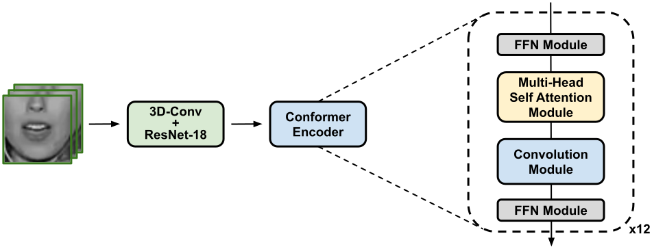
Figure 1: The overall architecture of our visual speech encoder. For simplicity, the initial layer normalization, the residual connection, and the final dropout of each module that compose the conformer encoder are omitted. Conv and FFN refer to Convolutional layer and Feed Forward Network, respectively.

3.3.   Conventional Hybrid Decoder

Morphological Model. The design of our conventional DNN-HMM decoder was based on the Wall Street Journal recipe provided by the Kaldi toolkit [Povey et al., 2011]. First of all, we estimated a preliminary GMM-HMM to obtain temporal alignments. Then, we applied the so-called HiLDA technique [Potamianos et al., 2001], reducing our visual speech features to a 40-dimensional latent representation.

Regarding our best DNN-HMM architecture, it consisted of two hidden layers of 1024 units, each followed by a Sigmoid activation function. We defined as input an 11-frame context window over the previous HiLDA features. The output layer dimension depended on the number of HMM-state labels defined by the preliminary GMM-HMM. Concretely: 3624, 3304, and 1968 HMM-state labels were defined for the LRS2-BBC, LRS3-TED, and LIP-RTVE corpora, respectively. Then, we estimated our DNN-HMM system based on a frame cross-entropy training [Hinton et al., 2012]. In average terms, each DNN-HMM decoder comprised around 4 million parameters.

Another important aspect was the HMM’s topology. Due to the lower sample rate presented by visual cues compared to acoustic signals, our first experiments focused on the optimal HMM’s topology. By adding transitions and/or reducing the number of states, we found that, in all cases, a 3-state left-to-right topology with skip transitions to the final state was the best approach to fit the temporary nature of our visual data.

Lexicon Model. For LRS2-BBC and LRS3-TED, we processed their corresponding training transcriptions with a phonemizer based on the CMU pronunciation dictionary. Similarly, for LIP-RTVE, we considered a phonemizer based on Spanish phonetic rules [Quilis, 1997]. However, the amount of training data of LIP-RTVE is not comparable to its English counterparts. For this reason, we used the text provided by the LIP-RTVE’s authors for the estimation of a language model, which offers around 80k phrases collected from different but contemporary TV newscasts. Thus, a set of 39 and 24 phonemes were defined for English and Spanish, respectively. In both cases, the default silence phones of Kaldi were then included.

Language Model. We used a 6-layer character-level Language Model (LM) based on the Transformer architecture [Vaswani et al., 2017]. A more detailed description about this Transformer-based LM can be found in Subsection 4.2.

However, for this conventional paradigm, we applied an approach based on a combination of one-pass decoding and lattice re-scoring [Lüscher et al., 2019]. Consequently, we used an auxiliary n-gram language model for decoding before re-scoring with the Transformed-based LM. Hence, a 3-gram word-level LM was also estimated. For each English database, we used the transcriptions included in its corresponding training set, while for LIP-RTVE, we considered the aforementioned 80k phrases. The estimated n-gram LMs offered 100.5, 112.8, and 113.4 test perplexities, with 25, 16, and 193 out-of-vocabulary words, for LRS2-BBC, LRS3-TED, and LIP-RTVE, respectively.

Decoding. The decoder is defined as a weighted finite-state transducer integrating the morphological, lexicon, and language models. Readers are referred to ?) for more details.

3.4.   CTC/Attention Decoder

Morphological Model. This state-of-the-art approach was implemented using the ESPNet toolkit [Watanabe et al., 2018]. Specifically, the decoder was composed of a 6-layer Transformer decoder [Vaswani et al., 2017] and a fully connected layer as the CTC-based decoding branch [Graves et al., 2006]. By combining both paradigms, the model is able to adopt both the Markov assumptions of CTC (an aspect in harmony with the speech nature) and the flexibility of the non-sequential alignments provided by the attention-based decoder. As proposed by ?), the loss function is defined as follows:

$$\mathcal{L}=\alpha\log p_{ctc}(\textbf{y}|\textbf{x})+(1-\alpha)\log p_{attn}(\textbf{y}|\textbf{x})$$ (1)

where $p_{ctc}$ and $p_{attn}$ denote the CTC and Attention posteriors, respectively. In both terms, x and y refer to the input visual stream and its corresponding character-level target, respectively. The $\alpha$ weight balances the relative influence of each decoder.

It should be noted that this end-to-end approach is based on a character-level speech recognition. For LRS2-BBC and LRS3-TED, we considered a set of 41 characters, while for LIP-RTVE we used a set of 37 characters. In both cases, special characters were included, such as the ‘space’ and the ‘blank’ symbols. On average, each CTC/Attention decoder comprised around 9.5 million parameters.

Language Model. We used a 6-layer character-level LM based on the Transformer architecture [Vaswani et al., 2017]. More details about how it was estimated are found in Subsection 4.2.

Decoding. The decoder integrates the attention- and CTC-based branches and the Transformer-based LM in a beam search process. Albeit it is the attention-based branch that leads this decoding process until predicting the end-of-sentence token, the rest of the components influence the search in a shallow fusion manner, as reflected in:

$$S=\lambda S_{ctc}+(1-\lambda)S_{attn}+\beta S_{lm}$$ (2)

where $S_{ctc}$ and $S_{attn}$ are the scores of the CTC and the Attention decoder, respectively, $\lambda$ is their corresponding relative weight, and $\beta$ and $S_{lm}$ refer to the LM influence weight and the LM score, respectively. Readers are referred to ?) for a more detailed description.

4.   Experimental Setup

Figure 2: Comparison in terms of performance (% WER) of the DNN-HMM and the CTC/Attention decoders based on the number of hours used to estimate both paradigms. The 9, 223, and 437 hours refers to the entire training set of the LIP-RTVE, LRS2-BBC, and LRS3-TED databases, respectively.

Experiments were conducted on a 12-core 3.50GHz Intel i7-7800X CPU and a GeForce RTX 2080 GPU with 8GB memory.

4.1.   Visual Speech Encoder

In most of our experiments, the visual speech encoder used the weights publicly released by ?) for the LRS2-BBC database, where more than 1000 hours of data from different databases (including the LRS3-TED corpus) were considered. Only in the case of the LIP-RTVE database, due to language mismatch, the encoder was fine-tuned by assembling the LRS2-BBC encoder and its corresponding CTC/Attention decoder pre-trained with the weights publicly released by ?) for the Spanish language. In order to represent the situation in a data-scarcity scenario, we only used 1 hour of data from the LIP-RTVE training set. Implementation details about this encoder fine-tuning process can be found in Subsection 4.3.

4.2.   Transformer Language Model

In our experiments, our Transformer-based LM (used both for the DNN-HMM lattice re-scoring and the CTC/Attention decoder) was pre-trained using the weights publicly released by Ma et al. [Ma et al., 2022] for both the English and Spanish language. Each of them was estimated using millions of characters collected from different databases corresponding to the language addressed. Nonetheless, it should be noted that, for the English LM, the transcriptions from the training sets of the LRS2-BBC and LRS3-TED databases were also considered. Therefore, to conduct a fair comparison, we fine-tuned the Spanish LM to the LIP-RTVE database using the 80k phrases provided by the original authors [Gimeno-Gómez and Martínez-Hinarejos, 2022]. Details on this LM fine-tuning process are described in Subsection 4.3. Considering the same character vocabularies described in Subsection 3.4, our LMs presented a character-level perplexity of around 3.0 for the corresponding test set of all the proposed databases. Each LM comprises around 50 million parameters.

4.3.   Training Process

Data Sets: the official splits were kept, with slight variations for the English corpora. For the LRS2-BBC, the pre-training and training sets were condensed into one training set, comprising a total of 223 hours. Similarly, the ‘pre-train’ and ‘train-val’ sets from the LRS3-TED were used as a 437-hours training set. In both cases, utterances with more than 600 frames were excluded, as considered by ?; ?).

Conventional Hybrid Decoder. Although we explored different training setups, the toolkit’s default settings specified in Karel’s DNN-HMM implementation provided the best recognition rates.

CTC/Attention Decoder. In all our experiments, we considered the settings specified by ?). Concretely, we used the Adam optimizer [Kingma and Ba, 2014] and the Noam scheduler [Vaswani et al., 2017] with 25,000 warmup steps during 50 epochs with a batch size of 16 samples, yielding a peak learning rate of 4$\times$10^-4. Regarding the CTC/Attention balance, we set the $\alpha$ weight of Equation 1 to 0.1.

Fine-Tuning Settings. The LM and the visual speech encoder were fine-tuned when addressing the LIP-RTVE database. In both cases, the AdamW optimizer [I.Loshchilov and Hutter, 2019] and a linear one-cycle scheduler [Smith and Topin, 2019] were used during 5 epochs, yielding a peak learning rate of 5$\times$10^-5. Due to our memory limitations, the batch size was set to 1 sample. We explored the accumulating gradient strategy [Ott et al., 2018], but no significant differences were found, possibly because the normalization layers were still affected by the actual reduced batch size.

4.4.   Inference Process

Conventional Hybrid Decoder. As considered by ?), we applied an approach based on a combination of one-pass decoding and lattice re-scoring. First of all, with a beam size of 18, we explored word insertion penalties from -5.0 to 5.0 and LM scales from 1 to 20. Once the best setting was determined, a lattice composed of the best 100 hypothesis for each test sample was obtained using the 3-gram word-level LM. Afterwards, the lattice was re-scored using the Transformer-based LM. In all the cases, the visual speech decoder was scaled by a factor of 0.1.

CTC/Attention Decoder. As considered by ?), we incorporated the Transformer-based LM in a shallow fusion manner. According to Equation 2, we set the $\beta$ weight to 0.6 and 0.4 for English and Spanish, respectively. For English, we set a word insertion penalty of 0.5 and a beam size of 40, while for Spanish, we set the word insertion penalty and the beam size to 0.0 and 30, respectively. Regarding the CTC/Attention balance, we set the $\lambda$ weight of Equation 2 to 0.1. It should be noted that we used the model averaged over the last 10 training epochs.

Evaluation Metric: Experiment results were reported in terms of the well-known Word Error Rate (WER) with 95% confidence intervals using the method described by ?).

5.   Results & Discussion

Training Hours DNN-HMM CTC/Attention % WER Time % WER Time 1 38.4$\pm$1.5 3.9 100.0$\pm$0.0 3.3 2 35.3$\pm$1.4 6.3 87.2$\pm$1.3 5.8 5 31.9$\pm$1.5 9.4 35.1$\pm$1.6 15.8 10 31.5$\pm$1.5 15.9 31.7$\pm$1.6 30.8 20 31.5$\pm$1.5 25.9 30.7$\pm$1.5 61.7 50 31.1$\pm$1.5 58.4 29.3$\pm$1.5 151.7 100 30.2$\pm$1.4 114.0 28.7$\pm$1.4 306.7 223 29.8$\pm$1.5 221.7 28.0$\pm$1.5 634.2

Table 1: Comparison of the DNN-HMM and the CTC/Attention decoders for the LRS2-BBC database based on the number of hours used to estimate both paradigms. System performance (% WER) and training time (Time) expressed in minutes are reported. The 223 training hours refer to the entire training set.

LRS2-BBC. Using the LRS2-BBC database is the ideal scenario, where the proposed encoder extracts the visual speech features for which it was explicitly trained. Table 1 reflects how the conventional paradigm is not only capable of obtaining state-of-the-art results, but also of significantly outperforming the CTC/Attention model in data-scarcity scenarios. Only when at least 10 hours of data were available, both approaches provided similar recognition rates. Besides, it should be mentioned that both paradigms presented a real time factor of around 0.75. However, despite offering a slightly better performance, the CTC/Attention estimation took more than twice the hybrid system training time.

Training Hours DNN-HMM CTC/Attention % WER Time % WER Time 1 70.7$\pm$1.1 4.4 100.0$\pm$0.0 2.5 2 67.1$\pm$1.2 7.0 100.0$\pm$0.0 5.0 5 59.4$\pm$1.3 9.4 98.0$\pm$1.8 13.3 10 57.4$\pm$1.4 15.5 67.2$\pm$1.7 25.8 20 55.7$\pm$1.5 26.6 58.8$\pm$1.7 52.5 50 54.8$\pm$1.4 60.6 53.1$\pm$1.8 130.8 100 54.6$\pm$1.4 115.5 50.9$\pm$1.8 261.7 200 53.7$\pm$1.4 229.0 50.3$\pm$1.7 524.2 437 53.5$\pm$1.5 358.2 50.0$\pm$1.7 820.0

Table 2: Comparison of the DNN-HMM and the CTC/Attention decoders for the LRS3-TED database based on the number of hours used to estimate both paradigms. System performance (% WER) and training time (Time) expressed in minutes are reported. The 437 training hours refer to the entire training set.

LRS3-TED. It is considered our domain-mismatch scenario. First, it should be noted that this corpus was used during the pre-training stage of the visual speech encoder. However, due to the data-driven nature of the encoder and the fact that it was later fine-tuned to the LRS2-BBC database, the resulting features were expected to be worse than those extracted for the aforementioned corpus. Nonetheless, it allowed us to study whether the consequences of this deterioration in the quality of visual speech features could be mitigated when a larger amount of data is available.

As Table 2 reflects, results comparable to state of the art (25-30% WER) were not achieved. Moreover, 20 hours were now necessary for both paradigms to offer a similar performance. The real time factor was around 0.82 and 0.75 for the DNN-HMM and CTC/Attention paradigm, respectively. Nonetheless, we can observe an analogous behaviour to that described for the LRS2-BBC database regarding data-scarcity scenarios, where the DNN-HMM would still be the best approach. Conversely, from 100 hours of data, the CTC/Attention showed significant differences w.r.t the conventional paradigm. It suggests that the state-of-the-art decoder could be more adaptable to poorer-quality speech representations.

However, the DNN-HMM and CTC/Attention decoders converge when the availability of more data does not imply any improvement in terms of performance (with 20 and 50 hours of training data, respectively, differences are not significant w.r.t. using all available data). This fact would demonstrate that the quality of the visual speech encoder is a real limitation whose consequences are not mitigated by decoders despite having larger amounts of data.

Training Hours DNN-HMM CTC/Attention % WER Time % WER Time 1 78.1$\pm$0.9 3.5 $>$100.0^$\dagger$ 2.5 2 77.5$\pm$1.0 5.5 $>$100.0^$\dagger$ 5.0 5 67.8$\pm$1.1 9.9 $>$100.0^$\dagger$ 12.5 9 66.2$\pm$1.1 16.6 89.0$\pm$1.2 23.3

• due to a peculiarity of the WER metric

Table 3: Comparison of the DNN-HMM and the CTC/Attention decoders for the LIP-RTVE database based on the number of hours used to estimate both paradigms. System performance (% WER) and training time (Time) in minutes are reported. The 9 training hours refer to the entire training set.

LIP-RTVE. In the case of the LIP-RTVE database, we were not only faced with a data-scarcity scenario, but also with a mismatch in terms of language. These could be the reasons why our first results were not acceptable. Therefore, we decided to adapt the visual speech encoder as if we were in the worst possible scenario of our experiments: when only 1 hour of data was available. As described in Subsection 3.2, we fine-tuned the encoder in an end-to-end manner, obtaining a baseline model capable of reaching results around 88.6% WER.

Results in Table 3 show that, as in the rest of the studied scenarios, the conventional DNN-HMM decoder outperforms its CTC/Attention counterpart. Using around 10 hours of data w.r.t. only 1 hour enhances around 15% WER in relative terms for the DNN-HMM system, which is in harmony with the roughly 18% relative improvement observed for the LRS2-BBC and LRS3-TED corpora. Furthermore, we argue that one of the reasons that could be behind the success of the DNN-HMM paradigm was the word-level LM influence.

We also investigated fine-tuning the entire end-to-end architecture using the whole training set of the LIP-RTVE database. Recognition rates of around 60% WER were obtained, which significantly improves the best performance obtained for the LIP-RTVE database to date. However, it should be noted that their estimate assumes more than six times the training time w.r.t the DNN-HMM model.

Overall Analysis. Figure 2 reflects how system performance degrades as visual speech features deteriorate from the ideal scenario (LRS2-BBC) to the language-mismatch (LIP-RTVE) scenario. This trend is not only an aspect we could expect, but it is also supported by Tseng et al. [Tseng et al., 2023], whose study demonstrated the lack of generalization of different audio-visual self-supervised speech representations in multiple tasks. However, the interesting finding is that the conventional DNN-HMM, compared to its state-of-the-art counterpart, offers a significantly more robust approach when the quality of our visual speech features is not optimal. If, for instance, we analyze the scenario with 5 hours of training data, we can observe how the performance gap between the DNN-HMM and CTC/Attention paradigms in the language- and domain-mismatch scenario is significantly greater than in ideal settings, making the DNN-HMM paradigm a more suitable option when addressing the task in data-scarcity scenarios and non-optimal visual speech features.

Findings. According to the findings of our case study, different aspects might be helpful for future researchers and developers focused on designing VSR systems in data-scarcity scenarios with limited computational resources. One of the main aspects is that, even in ideal scenarios with any type of limitation, DNN-HMM decoders not only reach state-of-the-art performance rates but also offer significantly lower training time costs. Furthermore, the fewer number of parameters composing it would facilitate the deployment of this type of system. Similarly, when we suffer from data scarcity and/or lack of optimal self-supervised speech representations for our specific conditions, the state-of-the-art CTC/Attention architecture would not be a recommendable option.

6.   Conclusions & Future Work

In this work, we presented, to the best of our knowledge, the first thorough comparative study on the conventional DNN-HMM decoder and its state-of-the-art CTC/Attention counterpart for the visual speech recognition task. Unlike those comparative studies focused on auditory-based ASR, we also systematically investigated how these different decoding paradigms behave based on the amount of data available for their estimation. As reflected in Figure 2, our results showed that the conventional approach achieved recognition rates comparable to the state of the art, significantly outperforming the CTC/Attention model in data-scarcity scenarios. In addition, the DNN-HMM approach offered valuable properties, such as reduced training time and fewer parameters. Finally, by exploring databases of different natures, experiments suggest that further research should still focus on improving the robustness of visual speech representations for data scarcity, as well as domain- and language-mismatch scenarios.

For this reason, one of our future lines of research is not only studying how state-of-the-art visual speech features can generalize to other tasks and domains, but also extending our work toward estimating and evaluating robust multi-lingual visual speech representations using the MuAViC benchmark [Anwar et al., 2023].

7.   Acknowledgements

This work was partially supported by Grant CIACIF/2021/295 funded by Generalitat Valenciana and by Grant PID2021-124719OB-I00 under project LLEER (PID2021-124719OB-100) funded by MCIN/AEI/10.13039/501100011033/ and by ERDF, EU A way of making Europe.

8.   Bibliographical References

References

- Afouras et al., 2018a Afouras, T., Chung, J. S., Senior, A., Vinyals, O., and Zisserman, A. (2018a). Deep audio-visual speech recognition. IEEE Transactions on PAMI, 44(12):8717–8727.
- Afouras et al., 2018b Afouras, T., Chung, J.-S., and Zisserman, A. (2018b). LRS3-TED: a large-scale dataset for visual speech recognition. arXiv preprint arXiv:1809.00496.
- Anwar et al., 2023 Anwar, M., Shi, B., Goswami, V., Hsu, W.-N., Pino, J., and Wang, C. (2023). MuAViC: A Multilingual Audio-Visual Corpus for Robust Speech Recognition and Robust Speech-to-Text Translation. In Proc. InterSpeech, pages 4064–4068.
- Bear and Harvey, 2016 Bear, H. and Harvey, R. (2016). Decoding visemes: Improving machine lip-reading. In ICASSP, pages 2009–2013. IEEE.
- Bear et al., 2014a Bear, H., Harvey, R., Theobald, B., and Lan, Y. (2014a). Resolution limits on visual speech recognition. In ICIP, pages 1371–1375. IEEE.
- Bear et al., 2014b Bear, H., Harvey, R., Theobald, B., and Lan, Y. (2014b). Which phoneme-to-viseme maps best improve visual-only computer lip-reading? In International Symposium on Visual Computing, pages 230–239. Springer.
- Besle et al., 2004 Besle, J., Fort, A., Delpuech, C., and Giard, M.-H. (2004). Bimodal speech: early suppressive visual effects in human auditory cortex. European journal of Neuroscience, 20(8):2225–2234.
- Bisani and Ney, 2004 Bisani, M. and Ney, H. (2004). Bootstrap estimates for confidence intervals in asr performance evaluation. In ICASSP, volume 1, pages 409–412.
- Bregler and Konig, 1994 Bregler, C. and Konig, Y. (1994). ”eigenlips” for robust speech recognition. ICASSP, ii:II/669–II/672.
- Chan et al., 2016 Chan, W., Jaitly, N., Le, Q., and Vinyals, O. (2016). Listen, attend and spell: A neural network for large vocabulary conversational speech recognition. In ICASSP, pages 4960–4964.
- Cox et al., 2008 Cox, S. J., Harvey, R. W., Lan, Y., Newman, J. L., and Theobald, B.-J. (2008). The challenge of multispeaker lip-reading. In AVSP, pages 179–184.
- Denby et al., 2010 Denby, B., Schultz, T., Honda, K., Hueber, T., Gilbert, J. M., and Brumberg, J. S. (2010). Silent speech interfaces. Speech Communication, 52(4):270–287.
- Dong et al., 2018 Dong, L., Xu, S., and Xu, B. (2018). Speech-transformer: A no-recurrence sequence-to-sequence model for speech recognition. In ICASSP, pages 5884–5888.
- Dungan et al., 2018 Dungan, L., Karaali, A., and Harte, N. (2018). The impact of reduced video quality on visual speech recognition. In ICIP, pages 2560–2564.
- Ezz et al., 2020 Ezz, M., Mostafa, A. M., and Nasr, A. A. (2020). A silent password recognition framework based on lip analysis. IEEE Access, 8:55354–55371.
- Fernandez-Lopez and Sukno, 2018 Fernandez-Lopez, A. and Sukno, F. M. (2018). Survey on automatic lip-reading in the era of deep learning. Image and Vision Computing, 78:53–72.
- Fernández-López and Sukno, 2017 Fernández-López, A. and Sukno, F. (2017). Optimizing phoneme-to-viseme mapping for continuous lip-reading in spanish. In International Joint Conference on Computer Vision, Imaging and Computer Graphics, pages 305–328. Springer.
- Gales and Young, 2008 Gales, M. and Young, S. (2008). The application of hidden Markov models in speech recognition. Now Publishers Inc.
- Gimeno-Gómez and Martínez-Hinarejos, 2021 Gimeno-Gómez, D. and Martínez-Hinarejos, C.-D. (2021). Analysis of Visual Features for Continuous Lipreading in Spanish. In Proc. IberSPEECH, pages 220–224.
- Gimeno-Gómez and Martínez-Hinarejos, 2022 Gimeno-Gómez, D. and Martínez-Hinarejos, C.-D. (2022). LIP-RTVE: An Audiovisual Database for Continuous Spanish in the Wild. In Proceedings of LREC, pages 2750–2758, June.
- Gimeno-Gómez and Martínez-Hinarejos, 2023 Gimeno-Gómez, D. and Martínez-Hinarejos, C.-D. (2023). Comparing speaker adaptation methods for visual speech recognition for continuous spanish. Applied Sciences, 13(11).
- Gonzalez-Lopez et al., 2020 Gonzalez-Lopez, J. A., Gomez-Alanis, A., Martín Doñas, J. M., Pérez-Córdoba, J. L., and Gomez, A. M. (2020). Silent speech interfaces for speech restoration: A review. IEEE Access, 8:177995–178021.
- Graves and Jaitly, 2014 Graves, A. and Jaitly, N. (2014). Towards end-to-end speech recognition with recurrent neural networks. In ICML, pages 1764–1772.
- Graves et al., 2006 Graves, A., Fernández, S., Gomez, F., and Schmidhuber, J. (2006). Connectionist temporal classification: labelling unsegmented sequence data with recurrent neural networks. In Proceedings of the 23rd ICML, pages 369–376.
- Gulati et al., 2020 Gulati, A., Qin, J., Chiu, C. C., Parmar, N., Zhang, Y., Yu, J., Han, W., Wang, S., Zhang, Z., Wu, Y., and Pang, R. (2020). Conformer: Convolution-augmented Transformer for Speech Recognition. In Proc. Interspeech, pages 5036–5040.
- He et al., 2016 He, K., Zhang, X., Ren, S., and Sun, J. (2016). Deep residual learning for image recognition. In CVPR, pages 770–778.
- Hinton et al., 2012 Hinton, G., Deng, L., Yu, D., Dahl, G. E., Mohamed, A., Jaitly, N., Senior, A., Vanhoucke, V., Nguyen, P., Sainath, T. N., and Kingsbury, B. (2012). Deep neural networks for acoustic modeling in speech recognition: The shared views of four research groups. Signal Processing Magazine, 29(6):82–97.
- I.Loshchilov and Hutter, 2019 I.Loshchilov and Hutter, F. (2019). Decoupled weight decay regularization. In ICLR.
- Juang and Rabiner, 1991 Juang, B. H. and Rabiner, L. R. (1991). Hidden markov models for speech recognition. Technometrics, 33(3):251–272.
- Juang, 1991 Juang, B. (1991). Speech recognition in adverse environments. Computer Speech & Language, 5(3):275–294.
- Karita et al., 2019 Karita, S., Chen, N., Hayashi, T., Hori, T., Inaguma, H., Jiang, Z., Someki, M., Soplin, N., Yamamoto, R., Wang, X., Watanabe, S., Yoshimura, T., and Zhang, W. (2019). A comparative study on transformer vs rnn in speech applications. In ASRU, pages 449–456.
- Kim et al., 2021 Kim, Y. J., Heo, H.-S., Choe, S., Chung, S.-W., Kwon, Y., Lee, B.-J., Kwon, Y., and Chung, J. S. (2021). Look Who’s Talking: Active Speaker Detection in the Wild. In Proc. Interspeech, pages 3675–3679.
- Kingma and Ba, 2014 Kingma, D. and Ba, J. (2014). Adam: A method for stochastic optimization. In Proc. of the 2nd ICLR.
- Liu et al., 2023 Liu, X., Lakomkin, E., Vougioukas, K., Ma, P., Chen, H., Xie, R., Doulaty, M., Moritz, N., Kolar, J., Petridis, S., Pantic, M., and Fuegen, C. (2023). Synthvsr: Scaling up visual speech recognition with synthetic supervision. In CVPR, pages 18806–18815.
- Lüscher et al., 2019 Lüscher, C., Beck, E., Irie, K., Kitza, M., Michel, W., Zeyer, A., Schlüter, R., and Ney, H. (2019). RWTH ASR Systems for LibriSpeech: Hybrid vs Attention. In Proc. Interspeech, pages 231–235.
- Ma et al., 2021a Ma, P., Mira, R., Petridis, S., Schuller, B., and Pantic, M. (2021a). LiRA: Learning Visual Speech Representations from Audio Through Self-Supervision. In Proc. Interspeech, pages 3011–3015.
- Ma et al., 2021b Ma, P., Petridis, S., and Pantic, M. (2021b). End-to-end audio-visual speech recognition with conformers. In ICASSP, pages 7613–7617.
- Ma et al., 2022 Ma, P., Petridis, S., and Pantic, M. (2022). Visual speech recognition for multiple languages in the wild. Nature Machine Intelligence, 4(11):930–939.
- Ma et al., 2023 Ma, P., Haliassos, A., Fernandez-Lopez, A., Chen, H., Petridis, S., and Pantic, M. (2023). Auto-avsr: Audio-visual speech recognition with automatic labels. In ICASSP, pages 1–5.
- Matthews et al., 2002 Matthews, I., Cootes, T. F., Bangham, J. A., Cox, S., and Harvey, R. (2002). Extraction of visual features for lipreading. IEEE Transactions on PAMI, 24(2):198–213.
- McGurk and MacDonald, 1976 McGurk, H. and MacDonald, J. (1976). Hearing lips and seeing voices. Nature, 264(5588):746–748.
- Mohri et al., 2008 Mohri, M., Pereira, F., and Riley, M. (2008). Speech recognition with weighted finite-state transducers. In Springer Handbook of Speech Processing, pages 559–584. Springer.
- Nemani et al., 2023 Nemani, P., Krishna, G. S., Supriya, K., and Kumar, S. (2023). Speaker independent vsr: A systematic review and futuristic applications. Image and Vision Computing, 138:104787.
- Ott et al., 2018 Ott, M., Edunov, S., Grangier, D., and Auli, M. (2018). Scaling neural machine translation. In Proc. of the 3rd Conference on Machine Translation, pages 1–9. ACL.
- Potamianos et al., 2001 Potamianos, G., Luettin, J., and Neti, C. (2001). Hierarchical discriminant features for audio-visual lvcsr. In ICASSP, volume 1, pages 165–168.
- Potamianos et al., 2003 Potamianos, G., Neti, C., Gravier, G., Garg, A., and Senior, A. W. (2003). Recent advances in the automatic recognition of audiovisual speech. Proc. of the IEEE, 91(9):1306–1326.
- Povey et al., 2011 Povey, D., Ghoshal, A., Boulianne, G., Burget, L., Glembek, O., Goel, N., Hannemann, M., Motlicek, P., Qian, Y., Schwarz, P., Silovsky, J., Stemmer, G., and Vesely, K. (2011). The kaldi speech recognition toolkit. In ASRU, number EPFL-CONF-192584.
- Prajwal et al., 2021 Prajwal, K., Momeni, L., Afouras, T., and Zisserman, A. (2021). Visual keyword spotting with attention. In British Machine Vision Conference (BMVC).
- Prajwal et al., 2022 Prajwal, K. R., Afouras, T., and Zisserman, A. (2022). Sub-word level lip reading with visual attention. In CVPR, pages 5162–5172.
- Quilis, 1997 Quilis, A. (1997). Principios de fonología y fonética españolas, volume 43 of Cuadernos de lengua española. Arco libros.
- Ramachandran et al., 2017 Ramachandran, P., Zoph, B., and Le, Q. V. (2017). Searching for activation functions. arXiv preprint arXiv:1710.05941.
- Shi et al., 2022 Shi, B., Hsu, W. N., Lakhotia, K., and Mohamed, A. (2022). Learning audio-visual speech representation by masked multimodal cluster prediction. arXiv preprint arXiv:2201.02184.
- Smith and Topin, 2019 Smith, L. N. and Topin, N. (2019). Super-convergence: very fast training of neural networks using large learning rates. In AI and ML for Multi-Domain Operations Applications, volume 11006, pages 369–386. SPIE.
- Son Chung et al., 2017 Son Chung, J., Senior, A., Vinyals, O., and Zisserman, A. (2017). Lip reading sentences in the wild. In Proc. of the CVPR, pages 6447–6456.
- Stafylakis and Tzimiropoulos, 2018 Stafylakis, T. and Tzimiropoulos, G. (2018). Zero-shot keyword spotting for visual speech recognition in-the-wild. In Proc. of the ECCV, pages 513–529.
- Tao et al., 2021 Tao, R., Pan, Z., Das, R., Qian, X., Shou, M., and Li, h. (2021). Is someone speaking? exploring long-term temporal features for audio-visual active speaker detection. In Proc. of the 29th ACM International Conference on Multimedia, page 3927–3935. Association for Computing Machinery.
- Thangthai and Harvey, 2017 Thangthai, K. and Harvey, R. (2017). Improving computer lipreading via dnn sequence discriminative training techniques. In Proc. Interspeech, pages 3657–3661.
- Thangthai, 2018 Thangthai, K. (2018). Computer lipreading via hybrid deep neural network hidden Markov models. Ph.D. thesis, University of East Anglia.
- Tseng et al., 2023 Tseng, Y., Berry, L., Chen, Y.-T., Chiu, I., Lin, H.-H., Liu, M., Peng, P., Shih, Y.-J., Wang, H.-Y., Wu, H., Huang, P.-Y., Lai, C.-M., Li, S.-W., Harwath, D., Tsao, Y., Watanabe, S., Mohamed, A., Feng, C.-L., and Lee, H.-Y. (2023). Av-superb: A multi-task evaluation benchmark for audio-visual representation models. arXiv preprint arXiv:2309.10787.
- Vaswani et al., 2017 Vaswani, A., Shazeer, N., Parmar, N., Uszkoreit, J., Jones, L., Gomez, A. N., Kaiser, L., and Polosukhin, I. (2017). Attention is all you need. NeurIPS, 30:6000–6010.
- Wang et al., 2019 Wang, D., Wang, X., and Lv, S. (2019). An overview of end-to-end automatic speech recognition. Symmetry, 11(8).
- Watanabe et al., 2017 Watanabe, S., Hori, T., Kim, S., Hershey, J. R., and Hayashi, T. (2017). Hybrid ctc/attention architecture for end-to-end speech recognition. IEEE JSTSP, 11(8):1240–1253.
- Watanabe et al., 2018 Watanabe, S., Hori, T., Karita, S., Hayashi, T., Nishitoba, J., Unno, Y., E. Y. Soplin, N., Heymann, J., Wiesner, M., Chen, N., Renduchintala, A., and Ochiai, T. (2018). ESPnet: End-to-End Speech Processing Toolkit. In Proc. Interspeech, pages 2207–2211.