Federated Multi-Task Learning on Non-IID Data Silos: An Experimental Study

Abstract.

The innovative Federated Multi-Task Learning (FMTL) approach consolidates the benefits of Federated Learning (FL) and Multi-Task Learning (MTL), enabling collaborative model training on multi-task learning datasets. However, a comprehensive evaluation method, integrating the unique features of both FL and MTL, is currently absent in the field. This paper fills this void by introducing a novel framework, FMTL-Bench, for systematic evaluation of the FMTL paradigm. This benchmark covers various aspects at the data, model, and optimization algorithm levels, and comprises seven sets of comparative experiments, encapsulating a wide array of non-independent and identically distributed (Non-IID) data partitioning scenarios. We propose a systematic process for comparing baselines of diverse indicators and conduct a case study on communication expenditure, time, and energy consumption. Through our exhaustive experiments, we aim to provide valuable insights into the strengths and limitations of existing baseline methods, contributing to the ongoing discourse on optimal FMTL application in practical scenarios. The source code will be made available for results replication.

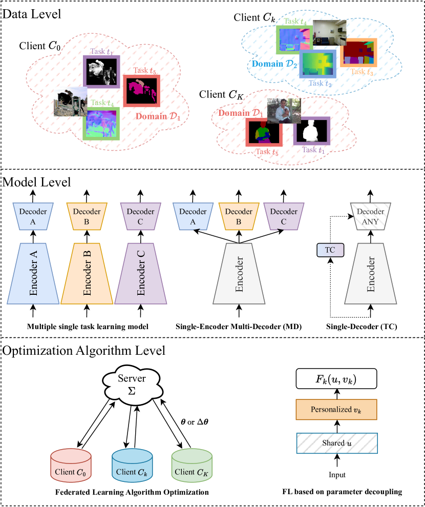
Figure 1. Design of Comparative Experimental Scenarios in FMTL-Bench. Refer to (Sec. 3.2) for detailed information.

Data Level: We design seven sets of experiments to cover main data partitioning scenarios in FMTL. These scenarios consider the different numbers and types of MTL tasks from various domains that a client may train. For more details, refer to Fig. 2. Model Level: We examine numerous single-task learning models and MTL models, the latter based on either multi-decoder (MD) or single-decoder architectures contingent on task conditions (TC). Experiments are conducted using network backbones of different sizes. The shaded sections in the figure represent task-agnostic parameters. Optimization Algorithm Level: We discuss nine baseline algorithms encompassing local training, FL, MTL, and FMTL algorithms. These algorithms leverage optimization based on either model parameters or accumulated gradients. Some baselines employ a parameter decoupling strategy and use model encoder as feature extractor during the FL process.

1. Introduction

Federated Multi-Task Learning (FMTL) (Zhuang et al., 2023; Lu et al., 2023), a burgeoning machine learning paradigm, facilitates collaborative model training on multi-task learning datasets of diverse sample sizes, domains, and task types while ensuring data locality. It marries the advantages of Federated Learning (FL) (Konečný et al., 2015; McMahan et al., 2017) and Multi-Task Learning (MTL) (Caruana, 1997), both extensively employed in sectors like medical imaging (Han et al., 2020; Kaissis et al., 2021, 2020; Bercea et al., 2022; Bai et al., 2021; Qi et al., 2023; Karargyris and otherss, 2023; Feng et al., 2024; Jin et al., 2021; Eyuboglu et al., 2021), healthcare (Warnat-Herresthal et al., 2021; Zhang et al., 2022; Dayan et al., 2021; Wu et al., 2023), and personalized recommendations (Wu et al., 2022a, b; Kalra et al., 2023). FMTL enables a single model to learn multiple tasks in a privacy-preserving, distributed machine learning environment, thereby inheriting and amplifying the challenges of both FL (Yang et al., 2019; Kairouz et al., 2021) and MTL (Vandenhende et al., 2021; Ruder, 2017; Crawshaw, 2020).

Early research (Mills et al., 2021; Liu et al., 2022; He et al., 2022; Smith et al., 2017; Marfoq et al., 2021) predominantly adopted MTL’s optimization strategy for personalized federated learning (PFL) (Tan et al., 2022) contexts. In non-independent and identically distributed (Non-IID or NIID) scenarios, each client’s personalized optimization objective function was treated as an individual task, with MTL optimization methods managing task heterogeneity arising from diverse client data. Classic machine learning tasks like image classification were commonly employed. A handful of studies (Park et al., 2021; Cai et al., 2023; Chen et al., 2023) have started probing more complex scenarios, aiming to allow clients to concurrently train different task types via FL. In some industrial contexts, such as autonomous driving (Janai et al., 2020), a single model must learn multiple distinct dense prediction tasks (Chen et al., 2018; Ranftl et al., 2021; Wang et al., 2021) (e.g., semantic segmentation, depth estimation, and surface normal estimation) simultaneously. The final scenario (Zhuang et al., 2023; Lu et al., 2023) involves learning an MTL model within a single client, which is the focus of this article.

However, the current research landscape of the FMTL paradigm is still in its infancy and has not fully integrated the characteristics of both FL and MTL to establish suitable scenarios and evaluation methods. The currently employed FL and MTL optimization algorithms and models are relatively simple, and there is a scarcity of experimental research to systematically comprehend FMTL task scenarios and baselines. Given growing interest in this technology, we introduce the FMTL-Bench to systematically evaluate the FMTL paradigm. Drawing from previous work on FL and MTL evaluation benchmarks (Li et al., 2022; Karargyris and otherss, 2023; Zhuang et al., 2023; Qiu et al., 2023; Vandenhende et al., 2021; Pieri et al., 2024; Hu et al., 2022), we integrated the strengths of these works to establish a comprehensive benchmark in the FMTL field, addressing data, model, and optimization algorithm levels for the first time. Contributions of our paper include:

• We meticulously consider the data, model, and optimization algorithm to design seven sets of comparative experiments.

• We amalgamate the characteristics of the two fields of multi-task learning and federated learning, conduct a case study, and extensively utilize a variety of evaluation methods to assess the performance of each baseline.

• We glean insights from comparative experiments and case analyses, and provide application suggestions for FMTL scenarios.

2. Methodology Overview

Suppose we have $K$ clients in total, Federated Learning (FL) (McMahan et al., 2017) is an optimization process that aims to minimize a global objective function. This function is defined by model parameters $\theta_{k}$, local objective function $\mathcal{L}_{k}$, and client weights $p_{k}$. In the Federated Multi-Task Learning (FMTL) scenario, each client manages a set of tasks $\mathcal{T}_{k}$ associated with a local dataset. The global function seeks to optimize personalized models for each client as expressed in Equation 1:

(1) $$\min_{\{\theta_{k}\}}\sum_{k\in[K]}p_{k}\mathcal{L}_{k}(\theta_{k}),\ \text{where\;}$$

$$\mathcal{L}_{k}(\theta_{k})=\frac{1}{\sum_{t\in\mathcal{T}_{k}}q_{k,t}}\sum_{t\in\mathcal{T}_{k}}q_{k,t}\ell_{k,t}(\theta_{k}).$$

In this equation, $\mathcal{L}_{k}$ is the local objective function. Weight $p_{k}$ of client $C_{k}$ in aggregation defaults to $\frac{1}{K}$, where $K$ is the total number of clients. Each task loss function $\ell_{k,t}(\theta_{k})$ is computed over the local dataset $\mathbb{D}_{k}$ of client $C_{k}$ for task $t$ in $\mathcal{T}_{k}$. The weights $q_{k,t}$ for each task $t$ default to $\frac{1}{|\mathcal{T}_{k}|}$, where $|\mathcal{T}_{k}|$ is the number of local tasks.

Multi-Task Learning (MTL) model level architecture design. To reduce the number of model parameters in MTL, a “single-encoder multi-decoder” (MD) architecture (Vandenhende et al., 2021) is often employed.

(2) $$\mathbf{y}_{n}=F_{k}^{\texttt{MD}}(\mathbf{x}_{n};\theta_{k}^{E},\sum_{t\in\mathcal{T}_{k}}\theta_{k,t}^{D}).$$

Here, $\mathbf{x}_{n}$ denotes the $n$-th input data, $\mathbf{y}_{n}$ is the corresponding output, $\theta_{k}^{E}$ denotes the encoder parameters of the $k$-th client model, and $\theta_{k,t}^{D}$ represents the decoder parameters for task $t$.

To further reduce the number of parameters, a “single-decoder based on task conditions” (TC) architecture (Maninis et al., 2019; Sun et al., 2021) is utilized.

(3) $$\mathbf{y}_{n,t}=F_{k}^{\texttt{TC}}(\mathbf{x}_{n};\theta_{k}^{E},\theta_{k}^{D},\theta_{k,t}^{T}),\quad\forall t\in\mathcal{T}_{k}.$$

In this equation, $\theta_{k}^{E}$ and $\theta_{k}^{D}$ are encoder and decoder parameters shared among all tasks $\mathcal{T}_{k}$, and $\theta_{k,t}^{T}$ are the task-specific parameters for task $t$ used in the conditioning strategy. In addition to architecture design, MTL also requires a lot of optimization work from the perspective of parameters and gradients (Vandenhende et al., 2021).

Federated learning (FL) algorithm optimization level. Parameter decoupling strategies are also frequently used in FL and FMTL scenarios to reduce communication expenses, manage with model task heterogeneity, and improve optimization performance. These strategies divide the model parameters into shared parameters $u$ and personalized parameters $v_{k}$ for client $k$.

(4) $$\min_{u,\{v_{k}\}}\sum_{k\in[K]}p_{k}\mathcal{L}_{k}(u,v_{k}).$$

In FL scenarios, sharing feature extractors between clients (Collins et al., 2021) is common, while in FMTL scenarios, the encoder serves as a default feature extractor (Chen et al., 2023; Cai et al., 2023). In addition to parameter decoupling strategy, we also verified the effects of various FL, PFL, MTL, and FMTL algorithms in subsequent experiments (see Sec. 3.2.3). We have introduced the core methodology, and due to space limitations, we will not discuss in detail the nine algorithms used in this article.

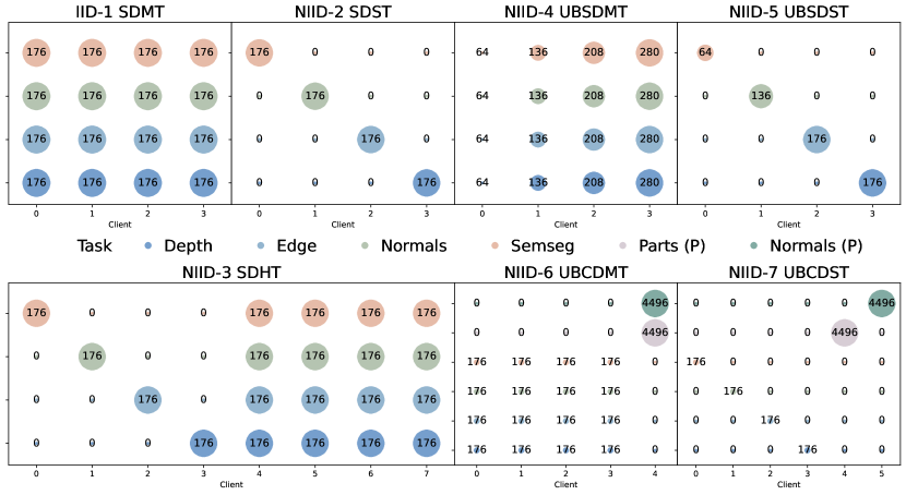
Figure 2. Data Level: Relationship diagram and Data Distribution of Comparative Experiments in Federated Multi-Task Learning.

This figure presents two levels of detail regarding our comparative experiments in federated multi-task learning. ‘MT’ represents Multi-Task, ‘ST’ stands for Single-Task, and ‘HT’ denotes Hybrid-Task. ‘SD’ signifies a single domain, while ‘CD’ refers to cross-domain. ‘UB’ is an abbreviation for unbalanced quantity. Left-hand side: an overview of the relationships between seven groups of comparative experiments is provided. This relationship diagram encapsulates the main scenarios of independent and identically distributed (IID) and non-independent and identically distributed (NIID) federated multi-task learning. Right-hand side: a visualization of the training data distribution for these seven sets of comparative experiments is displayed. Each subfigure corresponds to a different comparative experiment. The horizontal axis denotes the client ID, while the vertical axis, differentiated by color, represents various types of tasks. Task types include depth estimation (‘Depth’), edge detection (‘Edge’), surface normal estimation (‘Normals’), semantic segmentation (‘SemSeg’), and human parts segmentation (‘Parts’). Dataset comes from NYUD-v2 by default, and (P) represents using the PASCAL-Context. The relative size of the scatter points signifies the number of task samples, and the center of each point corresponds to the specific number of samples. For a detailed view, please zoom in.

3. Experiment Evaluation

This research aims to establish a comprehensive benchmark, referred to as FMTL-Bench, in the field of federated multi-task learning. We have designed a robust experimental setup with three key components: comparative experiment, case study, and suggestion.

3.1. Experimental Setup

Our experiments are conducted using the PyTorch framework (Paszke et al., 2019). The hardware setup comprises a server equipped with eight NVIDIA RTX2080Ti GPUs, while memory-intensive experiments are executed on two NVIDIA RTX4080 GPUs. The design of our experimental configurations is guided by previous studies (Maninis et al., 2019; Kanakis et al., 2020; Ye and Xu, 2022; Cai et al., 2023; Chen et al., 2023; Zhuang et al., 2023).

Optimization. Model optimization is achieved using the AdamW optimizer (Loshchilov and Hutter, 2019), with an initial learning rate and weight decay rate of 1e-4. The batch size is set to 8. A cosine decay learning rate scheduler (Loshchilov and Hutter, 2017) is employed with a warm-up phase of 5 rounds. Loss functions are chosen based on the task; cross-entropy loss for semantic segmentation and human parts segmentation, and $\mathcal{L}_{1}$ loss for surface normal estimation and depth estimation. Weighted binary cross-entropy loss for edge detection and the weights for positive and negative pixels are set to 0.8 and 0.2 for the NYUD-v2 dataset, and 0.95 and 0.05 for the PASCAL-Context dataset.

We adhere to the default settings for FL, PFL, MTL, and FMTL baselines (see Sec. 3.2.3) as recommended in the original papers or source codes. The number of local training epochs is set to 4 for the NYUD-v2 dataset and 1 for the PASCAL-Context dataset, based on dataset size. Maximum number of communication rounds is capped at 100. Source code will be made available to reproduce the results.

Datasets. Our experiments utilize the PASCAL-Context (Mottaghi et al., 2014) and NYUD-v2 (Silberman et al., 2012) datasets, both of which are widely recognized in FMTL research (Cai et al., 2023; Chen et al., 2023). For single-domain experiments, we employ the NYUD-v2 dataset, which includes 795 training and 654 testing images of indoor scenes. The dataset provides labels for depth estimation (‘Depth’), edge detection (‘Edge’), surface normal estimation (‘Normals’), and semantic segmentation (‘SemSeg’) tasks. In cross-domain experiments, we introduce the PASCAL-Context dataset, from which we obtain the same type of normal task (‘Normals’) as NYUD-v2 and a different type of human parts segmentation (‘Parts’). The PASCAL-Context dataset contains 4998 training images and 5105 testing images for edge detection, semantic segmentation, human parts segmentation, surface normal estimation, and saliency detection tasks. The original training set is randomly divided into each client according to the specified method. The local dataset obtained by the client is re-divided into a local training set and a test set at a ratio of 9:1. Global evaluation G-FL and local evaluation P-FL (Chen and Chao, 2022; Shi et al., 2023) are conducted on the original test set and each client’s dataset, respectively. Following (Maninis et al., 2019; Kanakis et al., 2020; Ye and Xu, 2022), we employ diverse data augmentation techniques such as random scaling, cropping, horizontal flipping, and color jittering to augment training dataset. Both training and evaluation stages incorporate image normalization.

3.2. Comparative Experiments

Our comparative experiments comprehensively consider data, model, and optimization algorithms levels, among others.

3.2.1. Data Level

We begin with the IID-1 SDMT (Single-Domain Multi-Task) experiment, an independent and identically distributed (IID) setup involving four clients, each possessing a non-overlapping dataset from the same domain for identical tasks. Motivated by the pathological partition scenario in federated learning (McMahan et al., 2017), we devised the NIID-2 SDST (Single-Domain Single-Task) scenario. In this setup, each client is responsible for a distinct task, representing an extreme case of federated multi-task learning. To examine the influence of the number of tasks within a client on the outcomes, we amalgamated the clients from the IID-1 and NIID-2 scenarios, leading to the NIID-3 SDHT (Single-Domain Hybrid-Task) scenario.

To investigate the impact of imbalanced data volume, we established the NIID-4 UBSDMT (Unbalanced Single-Domain Multi-Task) and NIID-5 UBSDST (Unbalanced Single-Domain Single-Task) scenarios, derived from the IID-1 and NIID-2 scenarios, respectively. For a comprehensive understanding of federated multi-task learning in cross-domain situations, we introduced the NIID-6 UBCDMT (Unbalanced Cross-Domain Multi-Task) and NIID-7 UBCDST (Unbalanced Cross-Domain Single-Task) scenarios. These scenarios involve clients from diverse fields, utilizing cross-domain data with unbalanced sample sizes, and exhibiting heterogeneous tasks and models. Refer to Fig. 2 for relationship diagram and visualization of training data distribution across comparative experiment groups.

Table 1. Enumeration of multi-task learning model parameters and computational complexity (FLOPs) for clients in IID-1 Single-Domain Multi-Task (SDMT) scenario from Tab. 2.

Ar	BN	Parameters (M)					FLOPs (G)
		Encoder	Decoder	TC module	Total	Encoder/Total	Per task	Total
MD	resnet	11.18	26.21	/	37.39	29.89%	-	272.14
TC	resnet	11.18	7.09	0.12	18.39	60.79%	75.47	301.88
MD	swin-t	27.52	52.28	/	79.80	34.49%	-	211.13
TC	swin-t	27.52	13.76	0.12	41.40	66.48%	71.01	284.04

3.2.2. Model Level

In alignment with the conventional practice of implementing an “encoder-decoder” model architecture in multi-task learning, our experimental design subscribes to this paradigm. We bifurcate the client model into the encoder and decoder.

In multi-task learning, the network typically shares a single encoder across multiple tasks. For this shared encoder, we employ a lightweight structure grounded on the pre-trained ResNet-18 (He et al., 2016). Additionally, we include pre-trained Swin-T (Liu et al., 2021a) in our experiments for comparative analysis. This backbone network is paired with a Fully Convolutional Network and the task-specific header.

The decoder component, on the other hand, can vary based on the architecture (Vandenhende et al., 2021). While the conventional “multi-decoder” (MD) architecture as Eq. 2 assigns a separate decoder to each task, we introduce an innovative “single-decoder based on task conditions” (TC) architecture (Maninis et al., 2019; Sun et al., 2021) as Eq. 3. This novel approach, applied in the context of FMTL, employs a single decoder that adjusts according to the specific conditions of each task.

3.2.3. Optimization Algorithm Level

Our experimental setup deploys a suite of nine optimization algorithms, covering gradient- and parameter-based strategies for MTL optimization, along with personalization and parameter decoupling strategies for FL. The baseline algorithms are categorized as follows: Firstly, the Local method, which solely operates on local dataset training, refraining from involvement in the federated learning process. Secondly, the Federated Learning Method, exemplified by FedAvg (McMahan et al., 2017). Thirdly, the category of Personalized Federated Learning Algorithms, encompassing FedProx (Li et al., 2020), FedAMP (Huang et al., 2021), and FedRep (Collins et al., 2021). Fourthly, Multi-Task Learning Algorithms, which includes PCGrad (Yu et al., 2020) and CAGrad (Liu et al., 2021b), both underpinned by gradient optimization techniques. Finally, the Federated Multi-Task Learning Algorithms, comprising the FMTL methods MaT-FL (Cai et al., 2023) and FedMTL (Smith et al., 2017).

It is noteworthy that PCAGrad (Yu et al., 2020) and CAGrad (Liu et al., 2021b) are adapted for multi-task optimization using accumulated gradients transmitted by clients during FL communication rounds. Besides, FedRep (Collins et al., 2021) and MaT-FL (Cai et al., 2023) employ a parameter decoupling strategy as Eq. 4 for optimization. By default, the model’s encoder serves as a feature extractor, and only this portion of the parameters is transmitted during the FL process. Furthermore, in the NIID-6 UBCDMT scenario from Tab. 7, due to the diversity in the number and types of tasks among different clients, the model based on the MD architecture exhibits heterogeneity. Consequently, for this scenario, FedProx, FedAMP, PCGrad, CAGrad, and the FedMTL algorithms are modified using parameter decoupling strategy. This implies that algorithms with the “-E” flag only transmit and utilize the parameters or accumulated gradient of model encoder for FL optimization.

3.2.4. Evaluation Criteria

In our comparative studies, we devise evaluative indicators that comprehensively reflect the unique attributes of individual tasks, the holistic performance of multi-task learning, and the diversity of test set origins.

Task-Specific Metrics: Each task type is evaluated using its appropriate metric. For example, depth estimation is assessed using the Root Mean Square Error (RMSE), while the test Loss is used for edge detection. The mean error (mErr) is utilized for surface normal estimation, and the mean Intersection over Union (mIoU) is applied for both semantic segmentation and human parts segmentation.

Comprehensive Multi-Task Performance: To provide a holistic evaluation of various algorithms, we compute weighted average per-task performance improvement (Maninis et al., 2019), relative to the target local training baseline without any aggregation. The calculation is now adjusted to incorporate individual task weights:

(5) $$\Delta\%=\frac{1}{\sum_{i=1}^{N}w_{i}}\sum_{i=1}^{N}(-1)^{l_{i}}w_{i}\frac{M_{\texttt{Fed},i}-M_{\texttt{Target},i}}{M_{\texttt{Target},i}}\times 100\%.$$

In this formula, $N$ signifies the task count, and $M_{\texttt{Fed},i}$ and $M_{\texttt{Target},i}$ denote the performance of task $i$ under federated learning techniques and the target local baseline, respectively. The variable $l_{i}$ equals 1 when a lower metric value is desirable for task $i$, and 0 otherwise. The weight assigned to task $i$, represented by $w_{i}$, denotes the importance or priority of each task within the FMTL framework. By default, all tasks are assigned equal weight, i.e., $w_{i}=1/N,\forall i$.

Table 2. Comparative Experiments: Single-Domain Multi-Task (SDMT) and Single-Domain Hybrid-Task (SDHT) Scenarios.  

Above: SDMT (IID-1) with four Multi-Task (MT) clients using NYUD-v2. Below: SDHT (NIID-3) with four MT and four single-task clients using NYUD-v2. Notations: ‘BN’ denotes Backbone Network, ‘Algo’ represents Optimization Algorithm, ‘Ar’ signifies Architecture, and ‘OOM’ is Out of Memory. G-FL and P-FL refer to evaluations using global and local test sets, respectively. ‘$\uparrow$’ indicates higher is better, ‘$\downarrow$’ implies lower is better. An asterisk (*) means actual results to be multiplied by $1E-2$. Values before and after ‘±’ represent the average and standard deviation of performance indicators from multiple clients. Light blue shading indicates a baseline for comparison. ‘$\Delta\%$’ denotes average per-task performance improvement relative to the target baseline. Unless otherwise noted, subsequent tables share these notations. Please refer to Fig. 2 for relationship diagrams and training data distribution visualizations across comparative experiments.

G-FL

P-FL

Depth

Edge

Normals

Semseg

Depth

Edge

Normals

Semseg

Scenario

BN

Algo

Ar

RSME*↓

Loss*↓

mErr↓

mIoU↑

${\Delta_{\textsc{G}}\%\uparrow}$

RSME*↓

Loss*↓

mErr↓

mIoU↑

${\Delta_{\textsc{P}}\%\uparrow}$

MD

81.41±1.95

4.76±0.01

26.44±0.23

23.36±0.54

0.00

91.28±12.93

4.79±0.07

26.35±1.39

24.74±0.91

0.00

Local

TC

81.34±1.47

4.80±0.01

26.72±0.34

22.14±0.27

-1.76

89.90±10.42

4.84±0.07

26.35±1.10

22.06±0.99

-2.59

MD

71.10±0.13

4.77±0.00

22.96±0.01

30.01±0.08

13.52

75.76±16.96

4.80±0.07

22.69±1.23

31.67±0.92

14.67

FedAvg

TC

70.23±0.35

4.83±0.01

22.19±0.05

30.90±0.30

15.15

73.80±13.00

4.86±0.07

22.02±0.96

31.13±2.60

14.99

MD

70.92±1.27

4.77±0.00

22.95±0.12

29.98±0.38

13.55

75.66±13.53

4.80±0.07

22.80±1.32

31.71±1.94

14.64

FedProx

TC

72.04±0.21

4.80±0.00

22.55±0.04

32.99±0.19

16.65

77.82±11.43

4.83±0.08

22.31±1.00

31.80±1.46

14.44

MD

81.30±2.58

4.75±0.00

26.47±0.24

23.49±0.45

0.20

92.24±13.78

4.79±0.07

26.41±1.25

23.55±1.39

-1.52

FedAMP

TC

79.88±2.04

4.78±0.00

26.20±0.31

22.78±0.45

-0.03

85.18±11.53

4.82±0.07

25.86±1.43

23.12±2.08

0.34

MD

79.22±0.99

4.75±0.00

25.89±0.15

23.73±0.50

1.64

88.55±13.90

4.79±0.07

25.55±1.30

24.37±1.74

1.13

MaT-FL

TC

75.85±4.83

4.78±0.00

24.85±0.55

25.06±1.45

4.93

85.78±11.97

4.82±0.07

24.89±1.54

26.14±2.82

4.15

MD

83.64±0.85

4.77±0.00

28.87±0.20

20.02±0.27

-6.61

90.49±12.06

4.81±0.07

28.10±1.93

20.58±1.15

-5.75

PCGrad

TC

120.74±5.01

4.99±0.03

31.31±0.64

17.83±0.84

-23.81

122.00±9.23

5.02±0.09

31.05±0.85

17.50±0.85

-21.39

MD

77.48±1.50

4.75±0.00

25.24±0.09

24.16±0.37

3.25

85.35±15.28

4.78±0.07

25.06±1.26

25.18±1.87

3.34

CAGrad

TC

77.13±0.80

4.84±0.01

24.16±0.17

24.60±0.36

4.38

82.00±12.09

4.88±0.08

24.11±0.94

24.69±1.71

4.15

MD

78.01±1.52

4.75±0.00

25.39±0.13

24.21±0.38

3.00

86.96±14.58

4.79±0.07

25.37±1.25

25.00±1.97

2.38

FedRep

TC

74.03±1.03

4.78±0.01

24.18±0.17

26.09±0.19

7.22

79.22±15.16

4.81±0.07

24.11±1.20

26.63±2.35

7.23

MD

81.19±1.80

4.76±0.00

26.43±0.11

23.35±0.38

0.07

91.60±13.28

4.79±0.07

26.06±1.02

24.18±1.99

-0.38

resnet

FedMTL

TC

80.99±0.85

4.78±0.01

26.35±0.27

22.72±0.61

-0.58

81.99±2.39

4.78±0.01

26.50±0.21

22.63±0.58

0.32

MD

72.56±0.75

4.73±0.00

24.51±0.13

33.89±0.53

15.97

79.29±13.61

4.76±0.07

24.58±1.03

33.33±3.24

13.80

Local

TC

77.54±2.18

4.75±0.00

25.19±0.26

29.55±0.52

9.05

84.64±11.69

4.78±0.07

25.19±0.92

30.03±2.00

8.32

MD

61.96±0.00

4.73±0.00

21.24±0.00

44.61±0.00

33.79

66.41±14.28

4.76±0.07

21.35±1.13

44.64±3.37

31.82

FedAvg

TC

65.82±0.15

4.76±0.00

21.14±0.01

41.94±0.05

29.68

69.09±12.07

4.78±0.07

21.17±1.06

43.33±3.25

29.83

MD

62.42±0.00

4.73±0.00

21.22±0.00

44.51±0.00

33.56

65.94±13.85

4.76±0.07

21.29±1.03

43.65±2.31

31.01

FedProx

TC

65.63±0.32

4.75±0.00

21.14±0.01

41.95±0.04

29.80

67.97±10.79

4.79±0.07

21.23±1.09

42.76±3.62

29.45

MD

72.25±0.95

4.73±0.00

24.49±0.14

33.92±0.34

16.12

80.04±11.34

4.76±0.07

24.39±1.17

33.37±4.09

13.82

FedAMP

TC

77.40±1.41

4.74±0.00

25.24±0.27

29.98±0.72

9.56

83.54±10.86

4.77±0.07

25.38±1.22

30.60±2.08

9.07

MD

70.29±0.51

4.73±0.01

23.99±0.09

34.74±0.28

18.07

77.41±12.33

4.76±0.07

23.82±1.01

34.01±4.06

15.72

MaT-FL

TC

74.43±3.58

4.74±0.00

24.22±0.47

32.37±1.81

13.99

81.65±12.53

4.78±0.07

24.13±0.78

31.31±2.95

11.43

MD

109.92±2.54

4.84±0.00

26.09±0.21

28.67±0.87

-3.16

109.76±14.45

4.88±0.07

26.14±0.84

29.40±2.71

-0.62

PCGrad

TC

93.46±7.97

4.88±0.02

26.03±0.16

31.78±0.67

5.07

100.31±17.26

4.92±0.07

26.00±0.70

30.17±2.31

2.67

MD

67.89±0.89

4.75±0.00

22.54±0.09

37.18±0.52

22.68

74.53±14.31

4.78±0.07

22.61±1.18

36.11±3.10

19.68

CAGrad

TC

74.67±4.00

4.78±0.00

22.23±0.05

35.07±0.58

18.48

79.42±13.01

4.81±0.07

22.32±0.88

35.46±2.94

17.80

MD

69.79±0.59

4.73±0.01

23.80±0.07

35.24±0.19

18.94

76.98±12.73

4.76±0.07

23.97±0.99

34.92±3.25

16.62

FedRep

TC

72.12±1.66

4.74±0.00

23.73±0.11

33.80±0.37

16.69

77.11±11.24

4.77±0.07

23.74±1.03

33.23±3.88

15.04

MD

OOM

OOM

OOM

OOM

OOM

OOM

OOM

OOM

OOM

OOM

IID-1 SDMT

swin-t

FedMTL

TC

77.34±1.51

4.75±0.00

25.17±0.18

30.03±0.41

9.64

81.42±11.29

4.78±0.07

25.17±0.96

30.11±1.40

9.30

Local

73.20±7.92

4.74±0.00

24.53±2.09

30.04±5.37

11.58

66.90±2.04

4.72±0.00

25.15±2.5

32.36±8.50

0.00

FedRep

71.63±4.33

4.74±0.00

24.02±1.15

30.36±3.95

12.89

56.94±0.25

4.74±0.03

22.80±1.12

33.24±5.44

6.63

MaT-FL

MD

73.14±7.28

4.75±0.00

24.71±2.30

30.01±5.78

11.34

63.67±5.69

4.74±0.03

25.29±3.06

30.33±8.04

-0.61

Local

72.45±7.57

4.76±0.01

24.18±2.38

29.16±5.13

11.10

65.19±2.64

4.74±0.03

24.59±2.72

33.35±9.74

1.85

FedAvg

70.32±0.14

4.80±0.00

21.94±0.01

33.26±0.04

18.05

50.89±8.28

4.78±0.05

19.57±0.98

42.26±3.78

18.86

FedRep

68.37±1.18

4.77±0.02

22.98±1.08

31.71±4.05

16.16

53.34±5.36

4.76±0.06

22.11±0.97

34.68±4.34

9.67

resnet

MaT-FL

TC

72.68±6.50

4.76±0.01

24.62±2.36

29.34±5.71

10.80

64.82±5.90

4.76±0.04

25.13±3.09

29.37±7.39

-1.72

Local

66.69±6.30

4.71±0.01

22.66±1.53

39.73±3.27

25.88

61.09±3.21

4.68±0.00

23.11±2.03

40.99±8.96

11.08

FedRep

64.71±3.77

4.72±0.00

22.59±1.14

40.78±2.40

27.62

54.25±1.92

4.71±0.03

21.95±1.35

43.08±7.32

16.24

MaT-FL

MD

66.81±6.57

4.72±0.00

21.74±0.75

39.64±3.99

26.56

59.90±6.68

4.71±0.03

19.74±0.02

39.80±8.19

13.79

Local

66.96±4.86

4.73±0.00

22.99±1.54

36.84±1.11

22.28

62.06±2.22

4.71±0.01

23.41±2.32

38.85±7.13

8.61

FedAvg

67.37±0.27

4.76±0.00

21.05±0.04

42.40±0.05

29.78

51.23±6.61

4.71±0.06

17.26±1.55

58.70±4.15

34.10

FedRep

65.95±2.63

4.73±0.01

22.61±1.02

39.68±3.07

25.99

56.37±1.25

4.72±0.05

21.58±0.74

42.41±5.66

15.25

NIID-3 SDHT

swin-t

MaT-FL

TC

67.82±2.75

4.73±0.01

23.48±1.96

36.47±2.25

21.16

61.71±1.96

4.73±0.05

23.71±2.74

36.87±6.31

6.80

Table 3. Comparative Experiment: NIID-2 Single-Domain Single-Task (SDST) scenario. In this scenario, each client holds data pertaining to distinct task types. Refer to Table 2 for notation definitions and comparison baseline.

			G-FL					P-FL
			Depth	Edge	Normals	Semseg		Depth	Edge	Normals	Semseg
BN	Algo	Ar	RSME*↓	Loss*↓	mErr↓	mIoU↑	${\Delta_{\textsc{G}}\%\uparrow}$	RSME*↓	Loss*↓	mErr↓	mIoU↑	${\Delta_{\textsc{P}}\%\uparrow}$
		SD	81.13	4.75	26.61	24.68	1.39	68.93	4.71	27.64	23.85	4.42
	Local	TC	80.02	4.75	26.55	24.03	1.09	67.82	4.71	27.31	23.61	4.79
		SD	114.71	4.80	31.84	13.89	-25.68	107.56	4.77	33.77	12.14	-24.13
	FedAvg	TC	79.34	4.77	26.85	23.27	0.10	72.17	4.73	27.97	23.50	2.76
		SD	114.95	4.81	31.65	13.97	-25.54	106.66	4.78	33.69	11.62	-24.38
	FedProx	TC	79.29	4.78	26.86	23.02	-0.22	75.87	4.74	28.01	21.92	0.06
		SD	79.90	4.74	26.64	24.85	1.97	69.39	4.70	27.47	23.46	4.11
	FedAMP	TC	79.52	4.75	26.77	24.10	1.11	69.86	4.71	27.82	23.35	3.48
		SD	81.10	4.74	27.02	24.46	0.83	69.81	4.71	28.40	22.67	2.26
	MaT-FL	TC	78.71	4.74	27.57	24.03	0.58	69.20	4.71	28.86	23.26	2.59
		SD	109.75	4.83	32.89	11.52	-27.84	102.94	4.80	34.06	10.51	-24.94
	PCGrad	TC	138.12	4.77	32.34	15.45	-31.51	130.30	4.73	33.93	14.64	-27.77
		SD	114.64	4.80	32.02	13.55	-26.19	108.57	4.77	33.99	12.50	-24.25
	CAGrad	TC	80.55	4.79	27.28	22.80	-1.29	75.44	4.75	28.14	19.97	-1.97
		SD	80.47	4.74	27.06	23.91	0.40	72.79	4.71	28.64	21.54	0.08
	FedRep	TC	79.09	4.74	27.40	23.87	0.46	73.76	4.71	28.91	23.64	1.68
		SD	79.89	4.75	26.49	25.16	2.40	67.72	4.71	27.54	22.75	3.73
resnet	FedMTL	TC	78.70	4.75	26.67	24.07	1.43	72.92	4.71	27.98	22.26	1.39
		SD	73.00	4.72	24.18	36.46	18.95	64.29	4.68	25.15	32.03	16.47
	Local	TC	71.81	4.73	24.52	35.73	18.16	64.27	4.69	25.72	31.72	15.57
		SD	106.96	4.76	28.80	24.25	-9.13	96.45	4.73	29.64	22.72	-6.27
	FedAvg	TC	71.61	4.74	24.93	34.49	16.45	67.61	4.70	25.90	31.26	13.97
		SD	108.05	4.76	28.47	25.46	-7.85	99.37	4.72	29.65	23.95	-5.78
	FedProx	TC	71.77	4.74	24.95	34.76	16.67	67.50	4.70	25.86	31.41	14.19
		SD	72.65	4.72	24.20	36.89	19.50	64.99	4.68	25.72	31.71	15.42
	FedAMP	TC	73.23	4.73	24.44	35.21	17.24	65.01	4.69	25.66	32.36	16.07
		SD	74.92	4.72	24.83	38.70	20.14	64.17	4.68	26.12	31.85	15.40
	MaT-FL	TC	75.07	4.73	25.08	36.23	17.16	70.06	4.68	26.44	31.88	13.52
		SD	113.43	4.78	29.32	26.79	-8.99	106.03	4.75	30.36	23.37	-9.02
	PCGrad	TC	146.54	4.77	28.47	31.94	-12.79	139.00	4.74	29.97	27.00	-13.96
		SD	105.23	4.77	28.00	24.60	-7.52	95.27	4.73	28.39	25.36	-2.09
	CAGrad	TC	72.12	4.75	24.73	34.94	16.92	70.28	4.71	26.24	29.94	11.53
		SD	71.90	4.72	25.09	35.93	17.86	63.53	4.68	26.34	30.53	14.03
	FedRep	TC	70.30	4.72	25.62	34.22	16.02	65.59	4.68	26.77	28.85	11.36
		SD	73.40	4.72	24.25	36.62	18.93	63.58	4.68	25.45	30.99	15.33
swin-t	FedMTL	TC	72.10	4.73	24.40	35.90	18.37	61.46	4.69	25.83	32.43	16.95

Table 4. Comparative Experiment: NIID-5 Unbalanced Single-Domain Single-Task (UBSDST) with ResNet backbone. Each client holds distinct task types and variable sample numbers. Notations and the target baseline are as defined in Tab. 2.

		G-FL					P-FL
		Depth	Edge	Normals	Semseg		Depth	Edge	Normals	Semseg
Algo	Ar	RSME*↓	Loss*↓	mErr↓	mIoU↑	${\Delta_{\textsc{G}}\%\uparrow}$	RSME*↓	Loss*↓	mErr↓	mIoU↑	${\Delta_{\textsc{P}}\%\uparrow}$
	SD	75.48	4.75	27.06	16.89	-5.64	66.87	4.68	27.93	13.14	-5.96
Local	TC	74.83	4.75	27.08	16.45	-5.93	64.11	4.68	27.78	13.83	-4.37
	SD	104.07	4.81	31.53	7.26	-29.26	96.73	4.75	32.40	7.82	-24.12
FedAvg	TC	75.98	4.78	27.61	15.41	-8.05	67.79	4.71	27.75	12.23	-7.12
	SD	105.09	4.81	31.70	7.20	-29.80	97.95	4.75	32.46	7.62	-24.71
FedProx	TC	76.94	4.78	27.49	14.72	-8.97	67.46	4.71	27.95	11.60	-7.85
	SD	75.34	4.74	27.03	16.89	-5.51	65.61	4.67	27.43	13.90	-4.32
FedAMP	TC	75.21	4.75	27.11	16.86	-5.63	67.18	4.68	28.07	14.16	-5.15
	SD	76.17	4.75	27.76	16.64	-6.78	64.14	4.68	28.78	12.54	-6.63
MaT-FL	TC	74.75	4.75	27.96	16.34	-6.85	63.11	4.67	28.99	14.60	-4.41
	SD	112.07	4.83	33.19	6.95	-33.73	110.01	4.77	33.81	7.10	-29.93
PCGrad	TC	122.28	4.90	31.72	12.07	-30.36	124.20	4.84	32.98	9.60	-30.87
	SD	107.69	4.82	31.76	7.38	-30.52	101.75	4.75	32.54	7.98	-25.47
CAGrad	TC	76.05	4.80	28.12	15.68	-8.37	68.97	4.72	28.73	12.77	-7.88
	SD	75.23	4.75	27.41	16.74	-6.05	68.96	4.68	27.92	14.36	-5.29
FedRep	TC	73.53	4.75	27.82	16.45	-6.23	70.33	4.69	28.99	13.54	-7.56
	SD	75.36	4.75	27.05	16.81	-5.68	64.54	4.68	27.58	12.89	-5.24
FedMTL	TC	74.35	4.75	27.16	16.65	-5.64	65.58	4.68	27.96	14.14	-4.63

Table 5. Comparative Experiment: NIID-7 Unbalanced Cross-Domain Single-Task (UBCDST) with ResNet backbone.

Symbols (P) represent PASCAL-Context dataset. The configuration for first four clients mirrors that of NIID-2 scenario detailed in Tab. 3. In addition, Clients 4 and 5 incorporate larger datasets from a different domain. Client 4 introduces a new task, human parts segmentation, while Client 5 undertakes surface normal estimation as Client 1. Light blue shading indicates baseline for comparison. Refer to Tab. 2 for other notations.

			Depth	Edge	Normals	Semseg	Parts(P)	Normals(P)
Eval	Algo	Ar	RSME*↓	Loss*↓	mErr↓	mIoU↑	mIoU↑	mErr↓	${\Delta\%\uparrow}$
		SD	80.38	4.75	26.55	24.64	55.01	14.57	0.00
	Local	TC	79.27	4.75	26.62	24.62	54.80	14.59	0.09
		SD	111.71	4.85	30.18	10.63	39.25	17.92	-27.21
	FedAvg	TC	81.30	4.81	25.96	22.57	50.38	15.65	-4.07
		SD	111.66	4.85	29.98	10.99	40.03	17.69	-26.33
	FedProx	TC	80.04	4.81	25.95	22.55	50.45	15.63	-3.77
		SD	80.42	4.75	26.55	24.77	55.07	14.58	0.09
	FedAMP	TC	79.60	4.75	26.61	24.19	54.78	14.60	-0.28
		SD	80.79	4.75	26.59	23.49	52.47	15.00	-2.15
	MaT-FL	TC	80.97	4.75	26.56	23.27	52.94	14.91	-2.07
		SD	113.39	4.86	31.13	8.49	34.67	19.07	-32.34
	PCGrad	TC	117.70	4.85	30.69	15.57	39.24	18.34	-25.91
		SD	111.52	4.84	29.85	10.82	39.71	17.99	-26.74
	CAGrad	TC	80.72	4.82	26.63	22.16	49.37	16.03	-5.42
		SD	80.44	4.75	26.62	23.60	52.36	15.02	-2.08
	FedRep	TC	78.17	4.75	26.77	23.54	52.52	14.99	-1.66
		SD	80.54	4.74	26.56	24.74	54.97	14.59	0.03
G-FL	FedMTL	TC	80.03	4.75	26.61	23.89	54.68	14.60	-0.61
		SD	69.08	4.71	27.14	22.44	54.28	14.24	0.00
	Local	TC	75.83	4.71	27.21	22.90	55.62	14.17	-0.84
		SD	103.69	4.82	31.81	9.43	38.11	17.45	-29.99
	FedAvg	TC	74.99	4.77	27.12	20.67	51.12	15.33	-5.19
		SD	102.58	4.83	31.71	10.07	38.50	17.30	-28.93
	FedProx	TC	73.09	4.77	27.17	19.61	49.88	15.33	-5.93
		SD	71.89	4.71	27.82	24.44	55.65	14.14	0.93
	FedAMP	TC	69.65	4.70	27.28	22.40	55.16	14.15	0.16
		SD	71.26	4.71	27.79	20.16	53.21	14.62	-3.39
	MaT-FL	TC	77.87	4.70	28.17	20.75	52.95	14.50	-4.69
		SD	107.86	4.83	32.36	8.84	34.36	18.91	-34.67
	PCGrad	TC	105.01	4.80	32.40	14.79	37.20	18.03	-27.58
		SD	102.67	4.81	32.04	10.01	37.76	17.51	-29.60
	CAGrad	TC	69.89	4.78	28.03	19.23	48.88	15.67	-6.71
		SD	71.55	4.71	28.01	21.04	52.51	14.65	-3.19
	FedRep	TC	74.10	4.71	28.34	22.58	53.08	14.54	-2.56
		SD	67.38	4.71	27.29	22.35	54.50	14.18	0.39
P-FL	FedMTL	TC	69.90	4.72	27.54	22.71	54.55	14.12	-0.05

Table 6. Comparative Experiment: NIID-4 Unbalanced Single-Domain Multi-Task (UBSDMT) scenario. This scenario mirrors the IID-1 as detailed in Tab. 2, with the sole distinction being an unbalanced distribution of total samples across different clients.

		G-FL					P-FL
		Depth	Edge	Normals	Semseg		Depth	Edge	Normals	Semseg
Algo	Ar	RSME*↓	Loss*↓	mErr↓	mIoU↑	${\Delta_{\textsc{G}}\%\uparrow}$	RSME*↓	Loss*↓	mErr↓	mIoU↑	${\Delta_{\textsc{P}}\%\uparrow}$
	MD	84.82±9.99	4.77±0.03	26.82±1.68	22.16±4.48	-2.74	91.08±20.63	4.81±0.11	26.70±2.52	22.32±6.16	-2.83
Local	TC	82.36±7.60	4.78±0.00	26.72±1.68	22.04±4.66	-2.07	87.42±18.66	4.82±0.10	26.67±2.54	22.48±6.57	-1.69
	MD	71.55±0.07	4.77±0.00	22.96±0.01	29.98±0.10	13.35	68.15±4.99	4.80±0.10	22.69±0.56	29.15±4.67	14.21
FedAvg	TC	74.57±1.25	4.82±0.02	22.57±0.02	30.48±0.45	13.06	69.68±4.83	4.85±0.10	22.16±0.47	26.76±4.00	11.62
	MD	71.55±0.12	4.77±0.00	22.95±0.02	29.79±0.09	13.16	67.39±4.93	4.80±0.10	22.50±0.46	28.45±3.87	13.89
FedProx	TC	72.68±1.18	4.82±0.02	22.56±0.02	30.23±0.45	13.39	70.78±7.83	4.85±0.10	22.34±0.48	26.94±3.07	11.33
	MD	84.86±10.09	4.77±0.03	26.85±1.68	22.00±4.41	-2.96	91.62±22.57	4.81±0.11	26.38±2.62	22.62±6.60	-2.37
FedAMP	TC	83.11±7.45	4.78±0.01	26.83±1.76	21.92±4.24	-2.54	85.32±14.26	4.81±0.10	26.78±2.70	21.78±5.42	-1.87
	MD	82.68±8.21	4.77±0.02	26.02±1.02	22.61±3.58	-0.85	86.93±18.93	4.80±0.11	25.70±1.66	23.31±5.86	0.31
MaT-FL	TC	78.31±4.16	4.78±0.01	25.62±0.89	23.94±3.62	2.24	82.91±13.85	4.82±0.11	25.28±1.42	23.25±5.28	1.65
	MD	141.20±11.51	4.86±0.01	29.04±0.88	14.55±1.27	-30.77	146.40±18.90	4.89±0.10	28.25±1.09	14.81±2.01	-27.46
PCGrad	TC	105.72±15.51	4.95±0.04	32.33±0.59	17.24±2.54	-20.58	107.12±17.75	4.99±0.09	32.43±1.37	16.53±3.74	-19.45
	MD	84.53±6.03	4.81±0.01	25.33±0.87	19.66±2.36	-4.13	86.12±15.21	4.85±0.10	25.14±1.24	20.51±3.80	-2.03
CAGrad	TC	79.71±3.73	4.86±0.01	24.48±0.82	23.59±3.29	2.10	78.93±6.44	4.89±0.10	24.20±1.20	23.18±5.55	3.32
	MD	81.55±8.21	4.77±0.02	25.62±1.08	23.03±3.63	0.33	84.27±17.17	4.80±0.11	25.50±1.81	23.11±5.93	1.03
FedRep	TC	77.41±5.02	4.78±0.01	24.93±0.95	24.67±4.05	3.95	75.64±10.29	4.82±0.10	24.54±1.63	24.00±5.49	5.10
	MD	85.10±9.98	4.77±0.02	26.85±1.66	21.92±4.32	-3.11	90.05±19.50	4.80±0.11	26.46±2.49	23.29±5.93	-1.28
FedMTL	TC	83.21±7.25	4.78±0.01	26.76±1.82	22.22±4.40	-2.18	86.52±16.15	4.82±0.10	26.22±2.22	21.77±6.11	-1.73

Table 7. Comparative Experiment: NIID-6 Unbalanced Cross-Domain Multi-Task (UBCDMT) with global evaluation G-FL.

The setup for the first four clients mirrors that of the IID-1 scenario as detailed in Table 2. Client 4 incorporates a larger dataset from a different domain, introducing a new task of human parts segmentation while also performing the same surface normal estimation task as Client 1. ‘NULL’ indicates the absence of such a baseline. The ‘-E’ flag is used when only the parameters of the model encoder or the accumulated gradient are transmitted and utilized for federated learning optimization. For additional notation definitions, please refer to Table 2 and Table 5.

			Depth	Edge	Normals	Semseg	Parts(P)	Normals(P)
BN	Algo	Ar	RSME*↓	Loss*↓	mErr↓	mIoU↑	mIoU↑	mErr↓	${\Delta_{\textsc{G}}\%\uparrow}$
	Local	MD	81.82±2.09	4.76±0.00	26.49±0.13	23.37±0.64	54.12	13.86	0.00
	Local	TC	80.44±1.86	4.78±0.01	26.43±0.17	22.72±0.40	52.54	13.78	-0.61
	FedAvg	MD	NULL	NULL	NULL	NULL	NULL	NULL	NULL
	FedAvg	TC	75.27±0.20	4.82±0.00	22.15±0.04	30.50±0.19	50.59	14.89	6.61
	FedProx-E	MD	78.55±1.17	4.76±0.00	25.14±0.20	23.61±0.55	54.08	14.11	1.37
	FedProx	TC	73.76±0.20	4.82±0.00	22.23±0.04	30.06±0.19	50.22	14.88	6.46
	FedAMP-E	MD	81.33±1.74	4.76±0.00	26.50±0.13	23.16±0.37	54.2	13.87	-0.04
	FedAMP	TC	80.49±1.58	4.78±0.01	26.47±0.16	22.48±0.54	53.05	13.84	-0.73
	MaT-FL	MD	79.33±0.92	4.76±0.00	25.48±0.48	23.24±0.51	54.21	14.06	0.84
	MaT-FL	TC	78.44±3.28	4.79±0.01	25.24±0.77	23.78±0.72	53.19	14.01	1.20
	PCGrad-E	MD	88.96±1.27	4.79±0.00	30.43±0.28	16.32±0.40	46.73	18.67	-17.13
	PCGrad	TC	96.21±1.95	4.94±0.02	32.90±0.43	16.86±0.47	43.75	24.84	-28.63
	CAGrad-E	MD	78.22±1.21	4.75±0.00	25.02±0.16	24.07±0.68	53.78	14.16	1.73
	CAGrad	TC	78.71±1.80	4.86±0.01	23.81±0.04	23.95±0.39	49.77	14.99	-0.32
	FedRep	MD	78.86±1.43	4.76±0.00	25.16±0.13	23.66±0.53	54.17	14.08	1.40
	FedRep	TC	75.41±1.38	4.78±0.01	24.52±0.09	24.94±0.48	52.87	14.05	2.98
	FedMTL-E	MD	82.02±1.96	4.76±0.00	26.50±0.12	23.14±0.30	53.84	13.86	-0.30
resnet	FedMTL	TC	80.61±1.38	4.78±0.01	26.43±0.18	22.88±0.61	52.69	13.81	-0.52
	Local	MD	72.34±1.14	4.73±0.01	24.4±0.13	33.83±0.38	54.42	13.67	11.13
	Local	TC	77.50±2.22	4.75±0.00	25.19±0.20	29.98±0.59	52.35	13.65	6.15
	FedAvg	MD	NULL	NULL	NULL	NULL	NULL	NULL	NULL
	FedAvg	TC	70.15±0.17	4.78±0.00	20.96±0.02	40.65±0.03	52.32	14.61	16.65
	FedProx-E	MD	70.89±1.19	4.73±0.00	23.92±0.05	33.91±0.37	55.22	14.13	11.48
	FedProx	TC	70.12±0.18	4.78±0.00	20.99±0.02	40.51±0.03	52.32	14.62	16.53
	FedAMP-E	MD	OOM	OOM	OOM	OOM	OOM	OOM	OOM
	FedAMP	TC	77.77±1.53	4.75±0.00	25.25±0.15	29.95±0.99	52.33	13.7	5.97
	MaT-FL	MD	71.48±0.59	4.73±0.00	23.96±0.19	33.41±0.85	55.42	14.05	11.14
	MaT-FL	TC	72.08±1.33	4.74±0.00	23.80±0.07	33.69±0.23	52.09	13.62	10.77
	PCGrad-E	MD	79.38±2.37	4.73±0.00	26.16±0.05	33.25±0.34	52.93	15.38	5.66
	PCGrad	TC	85.99±14.50	4.90±0.02	28.31±0.22	34.98±0.49	50.84	19.68	-2.21
	CAGrad-E	MD	69.90±0.82	4.73±0.01	23.67±0.06	34.57±0.33	55	14.21	12.14
	CAGrad	TC	75.34±8.49	4.81±0.01	21.97±0.02	34.15±0.86	51.1	14.69	9.75
	FedRep	MD	70.78±1.18	4.73±0.00	23.89±0.04	33.90±0.43	55.32	14.13	11.54
	FedRep	TC	72.93±1.22	4.75±0.00	23.91±0.07	31.54±0.58	53.01	14.2	8.55
	FedMTL-E	MD	OOM	OOM	OOM	OOM	OOM	OOM	OOM
swin-t	FedMTL	TC	77.30±2.03	4.75±0.00	25.23±0.17	29.70±0.54	52.32	13.64	5.97

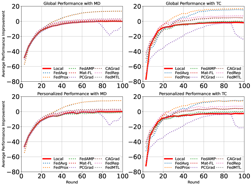
Figure 3. Case Study: Average task performance improvement (${\Delta\%\uparrow}$) versus communication rounds for baselines in IID-1 SDMT scenario from Tab. 2. Please zoom in for details.

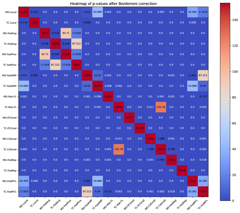
Figure 4. Case Study: Adjusted $p$-value heatmap for pairwise comparisons of baselines in IID-1 SDMT scenario from Tab. 2.

Heatmap displays adjusted $p$-values from pairwise comparisons, utilizing Wilcoxon signed-rank test with Bonferroni correction for multiple comparisons. Each cell corresponds to $p$-value from comparing the row and column baselines. $p$-values below 0.05, marked in white, signify a statistically significant performance difference between the pair of baselines. Please zoom in for details.

3.3. Case Study

Taking advantage of the unique characteristics of both multi-task learning and federated learning, we perform a case study using a variety of evaluation methods to assess baseline performances. These evaluation methods serve as a robust means for comparing the effectiveness of various algorithms and techniques. The case study complements the comparative experiments as an essential supplement (see Sec. 3.2.4).

3.3.1. Additional Evaluation Criteria in the Case Study

We have selected the IID-1 SDMT scenario in Tab. 2 as the primary focus of our case study. To meet the practical requirements of FMTL, we have structured our case study as follows:

Performance Improvement Over Time: Initially, we generate a curve that represents the evolution of the average per-task performance improvement, as defined by Eq. (5), as the number of federated learning communication rounds varies. This curve serves as a foundation for discussing the necessary number of rounds to achieve a specific target (see Fig. 3).

Metrics Recording and Analysis: We record key metrics such as communication overhead, energy consumption, and carbon emissions for each algorithm baseline. We then analyze these metrics in relation to the convergence speed of the algorithms (see Tab. 8).

Baseline Comparisons: Acknowledging the unique attributes of different MTL indicators, we first conduct a comparison of baselines using the average per-task performance improvement, a normalized singular metric. We also employ statistical methods, such as the Critical Difference (CD) Diagram (Demsar, 2006) with the Nemenyi post-hoc test (Sachs, 2013) (see Fig. 5) for comparing baselines across multiple metrics.

Influence of Pre-Training Strategy and Scalability: We include experiments where the model is trained from scratch. We also conduct experiments with varying numbers of clients, ranging from 2 to 8 (see Tab. 9).

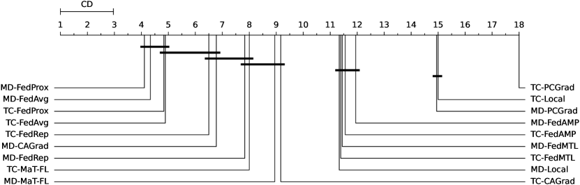
Figure 5. Case Study: the Critical Difference (CD) Diagram for baselines in IID-1 SDMT scenario from Table 2.

The CD Diagram (Demsar, 2006) illustrates the performance-based ranking of various baselines. Sorted from left (best) to right, baselines that are not significantly different according to Nemenyi post-hoc test (Sachs, 2013) are connected by horizontal lines. Please zoom in for details.

Table 8. Case Study: Comparison of communication costs (GB), energy consumption (kWh), training duration (min), and carbon dioxide emissions (g) for each baseline in the IID-1 Single-Domain Multi-Task (SDMT) scenario from Table 2.

$P$ is equipment running average power (W). $C_{r}$ and $T_{r}$ are communication overhead and running time (s) for each round respectively. $R_{30}$, $E_{30}$, $C_{30}$, and $T_{30}$ are respectively the number of communication rounds, energy consumption, communication costs, and time when the average task improvement reaches -30%, while $R_{10}$, $E_{10}$, $C_{10}$, and $T_{10}$ are for -10% improvement. $\texttt{CO}_{2}e$ refers to carbon dioxide emissions during training at -10% improvement. We refer to previous works (Zhuang et al., 2023; Qiu et al., 2023), and use the tool (Anthony et al., 2020) to record power, time, and carbon dioxide emissions on a server equipped with two NVIDIA RTX2080Ti GPUs and two Intel E5-2680V4 CPUs

Algo	Ar	$P$ (w)	$C_{r}$	$T_{r}$ (s)	$R_{30}$	$E_{30}$	$C_{30}$	$T_{30}$	$R_{10}$	$E_{10}$	$C_{10}$	$T_{10}$	$\texttt{CO}_{2}e$	${\Delta_{\textsc{G}}\%\uparrow}$
	MD	738.36	0.00	186.5	11	0.42	0.00	34	23	0.88	0.00	71	476.25	0.00
Local	TC	699.72	0.00	209.3	11	0.45	0.00	38	19	0.77	0.00	66	418.31	-1.76
	MD	745.99	1.17	189.0	11	0.43	12.85	35	23	0.90	26.87	72	487.62	13.52
FedAvg	TC	705.58	0.57	210.3	15	0.62	8.62	53	23	0.95	13.22	81	513.06	15.15
	MD	720.21	1.17	196.0	11	0.43	12.85	36	23	0.90	26.87	75	488.21	13.55
FedProx	TC	683.44	0.57	232.8	11	0.49	6.32	43	19	0.84	10.92	74	454.47	16.65
	MD	713.05	1.17	189.9	11	0.41	12.85	35	27	1.02	31.55	85	549.73	0.20
FedAMP	TC	710.36	0.57	215.3	7	0.30	4.02	25	27	1.15	15.52	97	620.80	-0.03
	MD	736.19	0.35	190.0	11	0.43	3.84	35	27	1.05	9.43	86	567.89	1.64
MaT-FL	TC	699.51	0.35	212.0	7	0.29	2.45	25	15	0.62	5.24	53	334.49	4.93
	MD	736.81	1.17	194.8	11	0.44	12.85	36	27	1.08	31.55	88	582.58	-6.61
PCGrad	TC	694.33	0.57	211.5	27	1.10	15.52	95	55	2.24	31.61	194	1214.51	-23.81
	MD	736.23	1.17	191.8	11	0.43	12.85	35	23	0.90	26.87	74	488.25	3.25
CAGrad	TC	703.17	0.57	212.0	11	0.46	6.32	39	23	0.95	13.22	81	515.57	4.38
	MD	738.90	0.35	188.0	11	0.42	3.84	34	23	0.89	8.04	72	480.43	3.00
FedRep	TC	706.55	0.35	208.8	7	0.29	2.45	24	19	0.78	6.64	66	421.39	7.22
	MD	692.65	4.67	202.6	11	0.43	51.41	37	23	0.90	107.50	78	485.35	0.07
FedMTL	TC	694.80	2.30	225.5	11	0.48	25.29	41	23	1.00	52.87	86	541.87	-0.58

Table 9. Case Study: Influence of client size and scratch training strategy on model performance.

SN denotes the scenario, while 2C-8C represent training sets evenly distributed among 2 to 8 clients. ATI refers to Average Task Performance Improvement (${\Delta\%\uparrow}$). The blue shading indicates the target baseline from IID-1 SDMT scenario in Tab. 2. Different bar colors and lengths in the upper table denote relative improvements of baselines across scenarios. In the lower table, ‘*’ indicates the use of scratch training strategy, with color brightness representing relative improvement. Refer to Tab. 2 for details.

3.4. Results and Suggestions

Our experimental findings provide valuable insights and recommendations for future studies and applications in the FMTL.

3.4.1. General Evaluation

In accordance with the “No Free Lunch” principle, our results from seven comparative experiments demonstrate that no single “algorithm-model” baseline consistently outperforms others across all experiments. In fact, the PCGard algorithm, designed to resolve gradient conflict issues, generally underperforms. We advise selecting a baseline method based on the specific requirements of the scenario.

Different types of tasks have distinct indicators, and the relative ratios of their standard deviations also vary considerably. This suggests that the difficulty of learning varies across tasks. Although we treated each task equally in our work, as per Eq. 5, we posit that in real-world FMTL scenarios, the value of labels for different tasks can vary. Consequently, data holders should select high-value labels based on their actual requirements.

3.4.2. Data Level Analysis

In the IID-1 scenario (Tab. 2, Fig. 3, Fig. 5), FedAvg and FedProx significantly outperform others.

Comparing the Local baseline of IID-1 in Tab. 2 and NIID-2 in Tab. 3, we observe that in a scenario where the number of labels for each task is balanced: multiple single-task learning models (each model only learns one task) can achieve better performance than a multi-task learning model. Furthermore, in three sets of pathological partition scenarios (NIID-2, NIID-5 in Tab. 4, NIID-7 in Tab. 5) where each client has only one task, the combination of FedAvg, FedProx and CAGrad with the SD (single-task MD) has extremely poor performance. FedAMP and FedMTL can achieve a slight G-FL improvement compared to the Local algorithm. The TC architecture suffers less performance loss than the SD architecture.

In the NIID-3 from Tab. 2 mixed task number scenario, all baselines, excluding MaT-FL, benefit from the addition of clients in terms of G-FL. The combination of FedAvg and FedProx algorithms with the TC architecture significantly improves the P-FL.

Compared with IID-1 in Tab. 2, the average task improvement indicator of NIID-4 in Tab. 6 for algorithms other than FedAvg and FedProx all decreased by 1 to 2 percentage points, suggesting that these two algorithms are relatively robust.

Two sets of cross-domain tasks (NIID-6 Tab. 7 and NIID-7 Tab. 5) are jointly trained with the larger PASCAL dataset. Compared with the original IID-1 scenario in Tab. 2, all baselines perform significantly worse in most tasks when evaluated using each task’s metrics. This indicates cross-domain tasks pose a challenge for FMTL, thereby necessitating design of additional optimization strategies.

3.4.3. Model Level Analysis

Model Architecture. As per Tab. 1, compared to the widely studied MD architecture (Vandenhende et al., 2021; Zhuang et al., 2023), the TC architecture (Maninis et al., 2019; Sun et al., 2021) trades time and computation for space. The MD architecture learns all task labels simultaneously during training, while the TC learns different task labels sequentially. Hence, the TC architecture utilizes fewer model parameters but significantly increases the computational load and training time (see Tab. 8). It also does not require a balanced number of task labels, making it more flexible. For FMTL scenarios, the computing and communication capabilities of the participants and the characteristics of their datasets are crucial considerations, and the two architectures offer different selection biases. Backbone Network. It’s noteworthy that using a larger backbone significantly improves model performance across all comparative experiments. Provided that device computing capability and inter-client communication bandwidth are sufficient, we recommend using a larger backbone network in FMTL scenarios to handle complex tasks.

3.4.4. Optimization Algorithm Level Analysis

As can be seen from NIID-6 Tab. 7, the parameter decoupling strategy can aid the MD architecture in performing FL in heterogeneous model scenarios. Simultaneously, it can resist optimization direction conflicts from the MTL process and reduce model performance losses. Also, as observed from the Tab. 8 experiment, it can significantly reduce communication expenses when the same accuracy is achieved.

3.4.5. Case Study

As illustrated in Tab. 9, Pre-training Strategy. Initiating training with a pre-trained model, rather than starting from scratch, can markedly improve the model’s training efficacy. This strategy can significantly decrease communication overhead, training time, and energy consumption. Scale Impact. When client data diminishes and number of clients escalates, the performance of all algorithms, excluding FedAvg and FedProx, declines significantly. These two algorithms exhibit notable performance improvements compared to Local baseline (especially when combined with TC). This suggests that in IID scenarios, FedAvg and FedProx are highly effective, and TC can also be a primary consideration.

FMTL encompasses numerous model performance evaluation metrics, with each task having separate indicators. In addition to the average task improvement as in Eq. 5, we introduce a statistical method in Fig. 5 to evaluate the ranking of different baselines across multiple indicators, thereby gaining a clear understanding of the strengths, weaknesses, and statistical differences among baselines.

FMTL also needs to consider real-world deployment issues. The average task improvement as a function of communication rounds was obtained in Fig. 3 and used in Tab. 8. In the latter, we comprehensively assess the energy consumption, carbon emissions, communication volume, and time consumption of all baselines. Different baselines utilize the federated learning system differently, and the resources used to achieve specified goals also vary. In the IID-1 scenario from Tab. 2, when reaching a -10% average task improvement, except for the outlier “PCGrad-TC”, the time, energy consumption, and carbon emissions of all other baselines are relatively close. The parameter decoupling strategy significantly reduces the communication cost. Future research could incorporate communication expenditure, energy consumption, and time as optimization objectives in real-life FMTL deployment. Due to paper length constraints, we have not listed all conclusions from other experiments. These will be discussed in detail in subsequent work.

4. Conclusion

The emerging paradigm of federated multi-task learning (FMTL) enables data owners to collaboratively train cross-domain multi-task learning (MTL) models without the need for transferring data from its original domain. To facilitate this, we have developed a benchmark, FMTL-Bench, which covers a wide range of settings at data, model, and optimization algorithm levels. We carried out seven sets of comparative experiments to encompass a broad spectrum of data partitioning scenarios. To cater to the practical implementation needs of federated learning (FL) scenarios and the multi-task evaluation requirements of MTL, we utilized a diverse array of evaluation methodologies in our case studies. Through comprehensive experimentation, we have outlined the strengths and weaknesses of existing baseline methods, providing valuable insights for future method selection.

- (1)
- Anthony et al. (2020) Lasse F. Wolff Anthony et al. 2020. Carbontracker: Tracking and Predicting the Carbon Footprint of Training Deep Learning Models. ICML Workshop on Challenges in Deploying and monitoring Machine Learning Systems.
- Bai et al. (2021) Xiang Bai et al. 2021. Advancing COVID-19 Diagnosis with Privacy-Preserving Collaboration in Artificial Intelligence. Nature Machine Intelligence 3, 12 (2021), 1081–1089.
- Bercea et al. (2022) Cosmin I. Bercea et al. 2022. Federated Disentangled Representation Learning for Unsupervised Brain Anomaly Detection. Nature Machine Intelligence 4, 8 (2022), 685–695.
- Cai et al. (2023) Ruisi Cai, Xiaohan Chen, Shiwei Liu, Jayanth Srinivasa, Myungjin Lee, Ramana Kompella, and Zhangyang Wang. 2023. Many-Task Federated Learning: A New Problem Setting and A Simple Baseline. In CVPR. 5037–5045.
- Caruana (1997) Rich Caruana. 1997. Multitask learning. Machine learning 28, 1 (1997), 41–75.
- Chen and Chao (2022) Hong-You Chen and Wei-Lun Chao. 2022. On Bridging Generic and Personalized Federated Learning for Image Classification. In ICLR.
- Chen et al. (2018) Liang-Chieh Chen et al. 2018. Encoder-decoder with atrous separable convolution for semantic image segmentation. In ECCV. 801–818.
- Chen et al. (2023) Yiqiang Chen, Teng Zhang, Xinlong Jiang, Qian Chen, Chenlong Gao, and Wuliang Huang. 2023. FedBone: Towards Large-Scale Federated Multi-Task Learning. CoRR abs/2306.17465 (2023).
- Collins et al. (2021) Liam Collins, Hamed Hassani, et al. 2021. Exploiting shared representations for personalized federated learning. In ICML. 2089–2099.
- Crawshaw (2020) Michael Crawshaw. 2020. Multi-task learning with deep neural networks: A survey. CoRR abs/2009.09796 (2020).
- Dayan et al. (2021) Ittai Dayan et al. 2021. Federated Learning for Predicting Clinical Outcomes in Patients with COVID-19. Nature Medicine 27, 10 (2021), 1735–1743.
- Demsar (2006) Janez Demsar. 2006. Statistical Comparisons of Classifiers over Multiple Data Sets. J. Mach. Learn. Res. 7 (2006), 1–30.
- Eyuboglu et al. (2021) Sabri Eyuboglu et al. 2021. Multi-task weak supervision enables anatomically-resolved abnormality detection in whole-body FDG-PET/CT. Nat Commun 12 (2021), 1880.
- Feng et al. (2024) Bao Feng, Jiangfeng Shi, et al. 2024. Robustly federated learning model for identifying high-risk patients with postoperative gastric cancer recurrence. Nat Commun 15 (2024), 742.
- Han et al. (2020) Tianyu Han et al. 2020. Breaking Medical Data Sharing Boundaries by Using Synthesized Radiographs. Science Advances 6, 49 (2020), eabb7973.
- He et al. (2022) Chaoyang He, Emir Ceyani, Keshav Balasubramanian, Murali Annavaram, and Salman Avestimehr. 2022. Spreadgnn: Decentralized multi-task federated learning for graph neural networks on molecular data. In AAAI, Vol. 36. 6865–6873.
- He et al. (2016) Kaiming He, Xiangyu Zhang, Shaoqing Ren, and Jian Sun. 2016. Deep residual learning for image recognition. In CVPR. 770–778.
- Hu et al. (2022) Sixu Hu, Yuan Li, Xu Liu, Qinbin Li, Zhaomin Wu, and Bingsheng He. 2022. The oarf benchmark suite: Characterization and implications for federated learning systems. ACM Transactions on Intelligent Systems and Technology 13 (2022), 1–32.
- Huang et al. (2021) Yutao Huang, Lingyang Chu, et al. 2021. Personalized cross-silo federated learning on non-iid data. In AAAI, Vol. 35. 7865–7873.
- Janai et al. (2020) Joel Janai et al. 2020. Computer vision for autonomous vehicles: Problems, datasets and state of the art. Foundations and Trends® in Computer Graphics and Vision 12, 1–3 (2020), 1–308.
- Jin et al. (2021) Cheng Jin et al. 2021. Predicting treatment response from longitudinal images using multi-task deep learning. Nat Commun 12 (2021), 1851.
- Kairouz et al. (2021) Peter Kairouz, H. Brendan McMahan, et al. 2021. Advances and Open Problems in Federated Learning. Found. Trends Mach. Learn. 14, 1-2 (2021), 1–210.
- Kaissis et al. (2021) Georgios Kaissis et al. 2021. End-to-End Privacy Preserving Deep Learning on Multi-Institutional Medical Imaging. Nature Machine Intelligence 3, 6 (2021), 473–484.
- Kaissis et al. (2020) Georgios A. Kaissis et al. 2020. Secure, Privacy-Preserving and Federated Machine Learning in Medical Imaging. Nature Machine Intelligence 2, 6 (2020), 305–311.
- Kalra et al. (2023) Shivam Kalra et al. 2023. Decentralized federated learning through proxy model sharing. Nat Commun 14 (2023), 2899.
- Kanakis et al. (2020) Menelaos Kanakis, David Bruggemann, Suman Saha, Stamatios Georgoulis, Anton Obukhov, and Luc Van Gool. 2020. Reparameterizing convolutions for incremental multi-task learning without task interference. In ECCV. 689–707.
- Karargyris and otherss (2023) Alexandros Karargyris and otherss. 2023. Federated benchmarking of medical artificial intelligence with MedPerf. Nat Mach Intell 5, 7 (2023), 799–810.
- Konečný et al. (2015) Jakub Konečný et al. 2015. Federated Optimization: Distributed Optimization Beyond the Datacenter. CoRR abs/1511.03575 (2015).
- Li et al. (2022) Qinbin Li, Yiqun Diao, Quan Chen, and Bingsheng He. 2022. Federated learning on non-iid data silos: An experimental study. In 2022 IEEE 38th International Conference on Data Engineering (ICDE). IEEE, 965–978.
- Li et al. (2020) Tian Li, Anit Kumar Sahu, Manzil Zaheer, Maziar Sanjabi, et al. 2020. Federated Optimization in Heterogeneous Networks. In MLSys.
- Liu et al. (2021b) Bo Liu, Xingchao Liu, Xiaojie Jin, Peter Stone, and Qiang Liu. 2021b. Conflict-Averse Gradient Descent for Multi-task learning. In NeurIPS. 18878–18890.
- Liu et al. (2022) Ken Liu, Shengyuan Hu, Steven Z Wu, and Virginia Smith. 2022. On privacy and personalization in cross-silo federated learning. NeurIPS 35 (2022), 5925–5940.
- Liu et al. (2021a) Ze Liu, Yutong Lin, Yue Cao, Han Hu, Yixuan Wei, Zheng Zhang, Stephen Lin, and Baining Guo. 2021a. Swin transformer: Hierarchical vision transformer using shifted windows. In ICCV. 10012–10022.
- Loshchilov and Hutter (2017) Ilya Loshchilov and Frank Hutter. 2017. Sgdr: Stochastic gradient descent with warm restarts. In ICLR.
- Loshchilov and Hutter (2019) Ilya Loshchilov and Frank Hutter. 2019. Decoupled Weight Decay Regularization. In ICLR.
- Lu et al. (2023) Yuxiang Lu, Suizhi Huang, Yuwen Yang, Shalayiding Sirejiding, Yue Ding, and Hongtao Lu. 2023. Towards Hetero-Client Federated Multi-Task Learning. CoRR abs/2311.13250 (2023).
- Maninis et al. (2019) Kevis-Kokitsi Maninis, Ilija Radosavovic, and Iasonas Kokkinos. 2019. Attentive single-tasking of multiple tasks. In CVPR. 1851–1860.
- Marfoq et al. (2021) Othmane Marfoq, Giovanni Neglia, Aurélien Bellet, Laetitia Kameni, and Richard Vidal. 2021. Federated Multi-Task Learning under a Mixture of Distributions. In NeurIPS. 15434–15447.
- McMahan et al. (2017) Brendan McMahan et al. 2017. Communication-Efficient Learning of Deep Networks from Decentralized Data. In AISTATS, Vol. 54. 1273–1282.
- Mills et al. (2021) Jed Mills et al. 2021. Multi-task federated learning for personalised deep neural networks in edge computing. TPDS 33, 3 (2021), 630–641.
- Mottaghi et al. (2014) Roozbeh Mottaghi et al. 2014. The role of context for object detection and semantic segmentation in the wild. In CVPR. 891–898.
- Park et al. (2021) Sangjoon Park et al. 2021. Federated Split Task-Agnostic Vision Transformer for COVID-19 CXR Diagnosis. In NeurIPS.
- Paszke et al. (2019) Adam Paszke et al. 2019. Pytorch: An imperative style, high-performance deep learning library. NeurIPS 32 (2019).
- Pieri et al. (2024) Sara Pieri, Jose Restom, Samuel Horvath, and Hisham Cholakkal. 2024. Handling Data Heterogeneity via Architectural Design for Federated Visual Recognition. NeurIPS 36 (2024).
- Qi et al. (2023) Tao Qi et al. 2023. Differentially private knowledge transfer for federated learning. Nat Commun 14 (2023), 3785.
- Qiu et al. (2023) Xinchi Qiu, Titouan Parcollet, Javier Fernández-Marqués, Pedro P. B. de Gusmao, Yan Gao, Daniel J. Beutel, Taner Topal, Akhil Mathur, and Nicholas D. Lane. 2023. A First Look into the Carbon Footprint of Federated Learning. J. Mach. Learn. Res. 24 (2023), 129:1–129:23.
- Ranftl et al. (2021) René Ranftl, Alexey Bochkovskiy, and Vladlen Koltun. 2021. Vision transformers for dense prediction. In ICCV. 12179–12188.
- Ruder (2017) Sebastian Ruder. 2017. An overview of multi-task learning in deep neural networks. CoRR abs/1706.05098 (2017).
- Sachs (2013) Lothar Sachs. 2013. Angewandte Statistik: Statistische Methoden und ihre Anwendungen. Springer-Verlag.
- Shi et al. (2023) Mingjia Shi et al. 2023. PRIOR: Personalized Prior for Reactivating the Information Overlooked in Federated Learning.. In NeurIPS.
- Silberman et al. (2012) Nathan Silberman et al. 2012. Indoor segmentation and support inference from rgbd images. In ECCV. 746–760.
- Smith et al. (2017) Virginia Smith, Chao-Kai Chiang, Maziar Sanjabi, and Ameet Talwalkar. 2017. Federated Multi-Task Learning. In NeurIPS. 4424–4434.
- Sun et al. (2021) Guolei Sun, Thomas Probst, Danda Pani Paudel, Nikola Popović, Menelaos Kanakis, Jagruti Patel, Dengxin Dai, and Luc Van Gool. 2021. Task switching network for multi-task learning. In ICCV. 8291–8300.
- Tan et al. (2022) Alysa Ziying Tan, Han Yu, Lizhen Cui, and Qiang Yang. 2022. Towards Personalized Federated Learning. IEEE Transactions on Neural Networks and Learning Systems (2022), 1–17.
- Vandenhende et al. (2021) Simon Vandenhende et al. 2021. Multi-task learning for dense prediction tasks: A survey. IEEE TPAMI 44, 7 (2021), 3614–3633.
- Wang et al. (2021) Wenhai Wang et al. 2021. Pyramid vision transformer: A versatile backbone for dense prediction without convolutions. In ICCV. 568–578.
- Warnat-Herresthal et al. (2021) Stefanie Warnat-Herresthal et al. 2021. Swarm Learning for Decentralized and Confidential Clinical Machine Learning. Nature 594, 7862 (2021), 265–270.
- Wu et al. (2022a) Chuhan Wu et al. 2022a. Communication-Efficient Federated Learning via Knowledge Distillation. Nature Communications 13, 1 (2022), 2032.
- Wu et al. (2022b) Chuhan Wu et al. 2022b. A Federated Graph Neural Network Framework for Privacy-Preserving Personalization. Nature Communications 13 (2022), 3091.
- Wu et al. (2023) Xiaosong Wu et al. 2023. Wearable in-sensor reservoir computing using optoelectronic polymers with through-space charge-transport characteristics for multi-task learning. Nat Commun 14 (2023), 468.
- Yang et al. (2019) Qiang Yang, Yang Liu, Tianjian Chen, and Yongxin Tong. 2019. Federated Machine Learning: Concept and Applications. ACM Trans. Intell. Syst. Technol. 10, 2 (2019), 12:1–12:19.
- Ye and Xu (2022) Hanrong Ye and Dan Xu. 2022. Inverted pyramid multi-task transformer for dense scene understanding. In ECCV. 514–530.
- Yu et al. (2020) Tianhe Yu, Saurabh Kumar, Abhishek Gupta, Sergey Levine, Karol Hausman, and Chelsea Finn. 2020. Gradient Surgery for Multi-Task Learning. In NeurIPS.
- Zhang et al. (2022) Angela Zhang et al. 2022. Shifting Machine Learning for Healthcare from Development to Deployment and from Models to Data. Nature Biomedical Engineering (2022), 1–16.
- Zhuang et al. (2023) Weiming Zhuang, Yonggang Wen, Lingjuan Lyu, and Shuai Zhang. 2023. MAS: Towards Resource-Efficient Federated Multiple-Task Learning. In ICCV. 23414–23424.