\textblockorigin

0mm0mm

Chain of Thought Empowers Transformers to Solve Inherently Serial Problems

Zhiyuan Li Stanford University Toyota Technological Institute at Chicago Hong Liu Stanford University Denny Zhou Google Tengyu Ma Stanford University
Abstract

Instructing the model to generate a sequence of intermediate steps, a.k.a., a chain of thought (CoT), is a highly effective method to improve the accuracy of large language models (LLMs) on arithmetics and symbolic reasoning tasks. However, the mechanism behind CoT remains unclear. This work provides a theoretical understanding of the power of CoT for decoder-only transformers through the lens of expressiveness. Conceptually, CoT empowers the model with the ability to perform inherently serial computation, which is otherwise lacking in transformers, especially when depth is low. Given input length $n$, previous works have shown that constant-depth transformers with finite precision $\mathsf{poly}(n)$ embedding size can only solve problems in $\mathsf{TC}^{0}$ without CoT. We first show an even tighter expressiveness upper bound for constant-depth transformers with constant-bit precision, which can only solve problems in ๐– ๐–ข0superscript๐– ๐–ข0\mathsf{AC}^{0}, a proper subset of $\mathsf{TC}^{0}$. However, with $T$ steps of CoT, constant-depth transformers using constant-bit precision and $O(\log n)$ embedding size can solve any problem solvable by boolean circuits of size $T$. Empirically, enabling CoT dramatically improves the accuracy for tasks that are hard for parallel computation, including the composition of permutation groups, iterated squaring, and circuit value problems, especially for low-depth transformers.

1 Introduction

Chain-of-Thought (CoT) reasoning, the technique of including intermediate steps besides the final answers, through promptingย (Wei etย al., 2022; Chowdhery etย al., 2022; Lampinen etย al., 2022; Kojima etย al., 2022; Zhou etย al., 2023) or finetuning (Cobbe etย al., 2021; Nye etย al., 2021; Chung etย al., 2022; Huang etย al., 2022), dramatically enhances the performance of large language models (LLMs) on various reasoning benchmarksย (Wang etย al., 2023; Lewkowycz etย al., 2022; Suzgun etย al., 2022; Shi etย al., 2023; Yao etย al., 2022; Drozdov etย al., 2022; OpenAI, 2023; Google, 2023). The success of CoT has even been extended to multi-modal QAย (Zhang etย al., 2023; Yang etย al., 2023) and code generationย (Chen etย al., 2022; Gao etย al., 2022). However, despite the evident empirical success, the fundamental mechanism of CoT remains largely elusive (Wang etย al., 2022a).

A natural potential explanation is the intermediate steps provide extra information to the LLMs about the tasks and the most efficient approach to solving the tasks, so that LLMs can imitate those steps and solve the tasks more effectively. However, intriguingly, the efficacy of generating thought steps extends to zero-shot CoT promptingย (Kojima etย al., 2022), where the LLMs are only simply instructed with the prompt โ€œletโ€™s think step by stepโ€, and to even using incorrect reasoning steps in the few-shot examplesย (Wang etย al., 2022a; Madaan & Yazdanbakhsh, 2022).

These observations suggest that in the original few-shot CoT settings, the form of CoT is as important as (if not more important than) the contents in them, because merely instructing the LLMs to generate the intermediate steps helps.

This paper aims to study why the form of CoT improves the reasoning capability of LLMs. Our hypothesis is that CoT allows for performing more serial computations that a vanilla transformer cannot do without CoT. We formulate and analyze this hypothesis through the lens of expressiveness with and without CoT. We adopt the language of circuit complexity to discuss the capability of transformers. Previous worksย (Liu etย al., 2022b; Merrill & Sabharwal, 2023b) have shown standard decoder-only transformers (that output answers directly) are efficient parallel computers and can only express functions computable in an $O(1)$-parallel run-time with threshold circuits, $\TC^{0}$, a computational model that allows the ๐– ๐–ญ๐–ฃ๐– ๐–ญ๐–ฃ\mathsf{AND}, $\mathsf{OR}$, $\mathsf{NOT}$ and ๐–ฌ๐– ๐–ฉ๐–ฎ๐–ฑ๐–จ๐–ณ๐–ธ๐–ฌ๐– ๐–ฉ๐–ฎ๐–ฑ๐–จ๐–ณ๐–ธ\mathsf{MAJORITY} function with multiple inputs to be computed efficiently in parallel. We first show a tighter upper bound (Theoremย 3.1) for expressiveness of constant-precision transformer โ€“ it can only express a proper subset class of $\TC^{0}$, $\AC^{0}$, where ๐–ฌ๐– ๐–ฉ๐–ฎ๐–ฑ๐–จ๐–ณ๐–ธ๐–ฌ๐– ๐–ฉ๐–ฎ๐–ฑ๐–จ๐–ณ๐–ธ\mathsf{MAJORITY} gates are not allowed. Our upper bound is also more realistic because it handles the rounding issue or iterative addition of floating point numbers, while most previous results essentially only work for fixed-point number addition.

We then show that transformers equipped with CoTโ€”allowing the transformer to auto-regressively generate a sequence of intermediate tokens before answering the questionsโ€”can solve complex problems that inherently require serial computations (assuming well-known conjectures in complexity theory). Intuitively, without CoT, the number of serial computations conducted by the transformer is bounded by the depth (which is considered as a fixed constant for this work), whereas with $T$ intermediate steps, the number of serial computations possible is boosted to $T$. Note that $T$ can easily increase as the sequence length increases where the depth is a fixed number that depends on the architecture.

Concretely, we prove that a constant-precision transformer with $T$ intermediate steps and embedding dimension logarithmic in the sequence length can express any functions computable by a circuit of size $T$ in Theoremย 3.3. Taking $T$ to be polynomial in the sequence length, the result suggests that transformers with polynomially many intermediate steps are capable of computing all circuits in with polynomial size, $\Ppoly$, a superclass of P. Theoremย 3.3 also implies that transformers with linearly many intermediate steps can compute all regular languages, including composition of non-solvable groups, like permutation group over five elements, $S_{5}$, which does not belong to $\AC^{0}$ and is also widely conjectured to be out of $\TC^{0}$. As such, CoT makes transformers with bounded depth and precision strictly more powerful.

To corroborate our theoretical analysis, we empirically evaluate the capability of transformers in solving four core problems: modular addition, permutation composition, iterated squaring, and circuit value problem. We learn transformers to solve these tasks with a large amount of synthetic data, with and without CoT, or with additional hint but not CoT. The modular addition belongs to $\TC^{0}$, meaning it can be easily solved in parallel. Liu etย al. (2022a) shows it is solvable by constant-depth transformers with log-precision and, indeed empirically depth 1 is sufficient for the parity problem (Modulo 2 addition). The other three tasks are all conjectured to require inherently serial computations. As expected, the vanilla transformer either requires a huge depth to solve these tasks (because the depth is the upper bound on the number of serial computation by transformers), or cannot solve the tasks at all. On the other hand, CoT can solve these tasks as long as the depth exceeds a small threshold. These experiments demonstrate CoT can provide more serial computations to solve complex reasoning tasks.

2 Notations and Preliminaries

We use $\mathbb{N}$ and $\mathbb{R}$ to denote the set of natural numbers and real numbers respectively. For any $n\in\mathbb{N}^{+}$, we define $[n]\triangleq\{1,2,\ldots,n\}$. We define $\mathsf{relu}(x)\triangleq\max(x,0)$. For vector $x$, we use $x_{a:b}$ to denote the vector containing coordinates of $x$ from position $a$ to position $b$. For matrix $M$, we define $M_{a_{1}:b_{1},a_{2}:b_{2}}$ to denote the submatrix by selecting rows from $a_{1}$ to $b_{1}$, columns from $a_{2}$ to $b_{2}$. We also use $a_{1}:$ to denote the subset of indices from $a_{1}$ to the end, $:b_{1}$ to denote the subset of indices from the beginning (1) to $b_{1}$ and $:$ to denote all indices. Given two non-negative functions $f,g$, we say $f(n)=O(g(n))$ (resp. $f(n)=\Omega(g(n))$) iff there exists $C>0$, such that for all $n\geq 0$, $f(n)\leq Cg(n)$ (resp. $f(n)\geq Cg(n)$). We use $\poly(n)\triangleq\{T:\mathbb{N}\to\mathbb{N}\mid\exists k>0,T(n)=O(n^{k})\}$ to denote the set of functions with at most polynomial growth rate.

We use $\phi(x)=\sum_{i=1}^{|x|}2^{|x|-i}x_{i}$ to denote the value of binary number represented by binary string $x$. We use $\mathsf{bin}_{k}(x)$ to denote the usual binary encoding of natural number $x$ using $k$ binary bits in the sense that $\phi(\mathsf{bin}_{k}(x))=x$ and $\mathsf{sbin}_{k}(x)$ to denote the signed binary encoding, which is $2\mathsf{bin}_{k}(x)-(1,\ldots,1)$. For any $n\in\mathbb{N}^{+}$, we define $\mathrm{softmax}:\mathbb{R}^{n}\to\mathbb{R}^{n}$ as $(\mathrm{softmax}(x))_{i}=\exp(x_{i})/\sum_{i=1}^{n}\exp(x_{i})$ for any $x\in\mathbb{R}^{n}$ and $i\in[n]$. We use $\odot$ to denote the element-wise product of two vectors. We use $a\|b$ or $(a,b)$ to denote the concatenation of two vectors $a$ and $b$.

2.1 Decoder-only Transformers

Given a vocabulary ${\mathcal{V}}$ , a decoder-only transformer with parameter $\theta$ and maximal input length $n_{\max}$ maps a sequence of input tokens $(x_{1},\ldots,x_{n})\in{\mathcal{V}}^{n}$ to a probability distribution over ${\mathcal{V}}$ for all $n\leq n_{\max}$, denoted by $p_{\theta}(\cdot\mid x_{1},\ldots,x_{n})$. We also define function $\mathsf{TF}_{\theta}(x)$ by the token in ${\mathcal{V}}$ that maximizes $p_{\theta}(\cdot\mid x_{1},\ldots,x_{n})$, that is, $\mathsf{TF}_{\theta}(x)\triangleq\operatorname*{arg\,max}_{x\in{\mathcal{V}}}p_{\theta}(x\mid x_{1},\ldots,x_{n})$.

Next-token Generator:

Given a vocabulary ${\mathcal{V}}$, a next-token generator with parameter $\theta$ and maximal input length $n_{\max}$ is a mapping from $\cup_{n=1}^{n_{\max}}{\mathcal{V}}^{n}$ to ${\mathcal{V}}$. The main next-token generator we are interested in this work is decoder-only transformers, $\mathsf{TF}_{\theta}(x_{1},\ldots,x_{n})$ where $x_{i}\in{\mathcal{V}}$ for all $i\in[n]$. We also recursively define $\mathsf{TF}^{i}_{\theta}(x_{1},\ldots,x_{n})\triangleq\mathsf{TF}^{i-1}_{\theta}(x_{1},\ldots,x_{n},\mathsf{TF}_{\theta}(x_{1},\ldots,x_{n}))$, for every positive integer $i$ and $n$ satisfying that $i+n\leq n_{\max}-1$ with the base case that $\mathsf{TF}^{1}_{\theta}(x_{1},\ldots,x_{n})\triangleq\mathsf{TF}_{\theta}(x_{1},\ldots,x_{n})$. In other words, for all $0\leq i\leq n_{\max}-n-1$, the output with $i$ steps of CoT is $x_{n+i+1}=\mathsf{TF}^{i+1}_{\theta}(x_{1},\ldots,x_{n})=\mathsf{TF}_{\theta}(x_{1},\ldots,x_{n},x_{n+1},\ldots,x_{n+i})$.

Transformer Architecture Overview:

The decoder-only transformer model we consider in this paper is very similar to GPT style architecturesย (Radford etย al., 2019) and consists of four parts: a token embedding layer ($\mathsf{TE}$), a position encoding layer ($\mathsf{PE}$), an output linear layer ($\mathsf{OUTPUT}$), and a stack of $L$ identical layers serving as the โ€œdecoderโ€ where $L$ is also called the depth of the model. Each decoder layer has two sub-layers: a multi-head self-attention layer (๐– ๐–ณ๐–ณ๐–ญ๐– ๐–ณ๐–ณ๐–ญ\mathsf{ATTN}) and a position-wise fully-connected feed-forward network ($\mathsf{FF}$). Each layer mentioned above has its own trainable parameters and is indexed by the layer name and the depth for attention and feedforward layers. 111We ignore the LayerNormย (Ba etย al., 2016) in the usual transformer architecture for simplicity. Our expressiveness analysis can extend to the transformers with LayerNorm with more careful treatment. See Sectionย F.1 for discussion. That is we can split the model parameter $\theta$ in the following way: ฮธ=(ฮธ๐–ฏ๐–ค,ฮธ๐–ณ๐–ค,ฮธ๐–ฎ๐–ด๐–ณ๐–ฏ๐–ด๐–ณ,{ฮธ๐– ๐–ณ๐–ณ๐–ญ(l),ฮธ๐–ฅ๐–ฅ(l)}l=0Lโˆ’1)๐œƒsubscript๐œƒ๐–ฏ๐–คsubscript๐œƒ๐–ณ๐–คsubscript๐œƒ๐–ฎ๐–ด๐–ณ๐–ฏ๐–ด๐–ณsuperscriptsubscriptsubscriptsuperscript๐œƒ๐‘™๐– ๐–ณ๐–ณ๐–ญsubscriptsuperscript๐œƒ๐‘™๐–ฅ๐–ฅ๐‘™0๐ฟ1\theta=(\theta_{\mathsf{PE}},\theta_{\mathsf{TE}},\theta_{\mathsf{OUTPUT}},\{\theta^{(l)}_{\mathsf{ATTN}},\theta^{(l)}_{\mathsf{FF}}\}_{l=0}^{L-1}), which are all trainable. (See formal definition in Algorithmย 2). Throughout this paper, we use $d$ to denote the embedding size of a transformer.

Self-Attention Mechanism:

Given attention parameter ฮธ๐– ๐–ณ๐–ณ๐–ญ=(WQ,WK,WV,WO)โˆˆโ„dร—dร—โ„dร—dร—โ„dร—dร—โ„dร—dsubscript๐œƒ๐– ๐–ณ๐–ณ๐–ญsubscript๐‘Š๐‘„subscript๐‘Š๐พsubscript๐‘Š๐‘‰subscript๐‘Š๐‘‚superscriptโ„๐‘‘๐‘‘superscriptโ„๐‘‘๐‘‘superscriptโ„๐‘‘๐‘‘superscriptโ„๐‘‘๐‘‘\theta_{\mathsf{ATTN}}=(W_{Q},W_{K},W_{V},W_{O})\in\mathbb{R}^{d\times d}\times\mathbb{R}^{d\times d}\times\mathbb{R}^{d\times d}\times\mathbb{R}^{d\times d}, we define the Attention layer with mask for decoder-only transformer in Algorithmย 3. Note allowing multi-head attention will not change the class of problems solvable by constant layer decoder-only transformers as we can simulate 1 multi-head attention layer with any constantly many heads with multiple single-head attention layers. Thus for simplicity of presentation, we do not include multi-head attention in the definition below.

Algorithm 1 Causal Self-Attention, ๐– ๐–ณ๐–ณ๐–ญ๐– ๐–ณ๐–ณ๐–ญ\mathsf{ATTN}
1:Parameter ฮธ๐– ๐–ณ๐–ณ๐–ญ=(WQ,WK,WV,WO)subscript๐œƒ๐– ๐–ณ๐–ณ๐–ญsubscript๐‘Š๐‘„subscript๐‘Š๐พsubscript๐‘Š๐‘‰subscript๐‘Š๐‘‚\theta_{\mathsf{ATTN}}=(W_{Q},W_{K},W_{V},W_{O}), Input embedding $h=(h_{1},\ldots,h_{n})\in\mathbb{R}^{nd}$.
2:Output embedding hโ€ฒ=(h1โ€ฒ,โ€ฆ,hnโ€ฒ)โ‰œ๐– ๐–ณ๐–ณ๐–ญฮธ๐– ๐–ณ๐–ณ๐–ญโ€‹(h1,โ€ฆ,hn)superscriptโ„Žโ€ฒsubscriptsuperscriptโ„Žโ€ฒ1โ€ฆsubscriptsuperscriptโ„Žโ€ฒ๐‘›โ‰œsubscript๐– ๐–ณ๐–ณ๐–ญsubscript๐œƒ๐– ๐–ณ๐–ณ๐–ญsubscriptโ„Ž1โ€ฆsubscriptโ„Ž๐‘›h^{\prime}=(h^{\prime}_{1},\ldots,h^{\prime}_{n})\triangleq\mathsf{ATTN}_{\theta_{\mathsf{ATTN}}}(h_{1},\ldots,h_{n}).
3:$q_{i}\triangleq W_{Q}h_{i},k_{i}\triangleq W_{K}h_{i},v_{i}\triangleq W_{V}h_{i},\forall i\in[n]$
4:siโ‰œsoftmaxโ€‹(โŸจqi,k1โŸฉ,โ€ฆ,โŸจqi,kiโŸฉ)โˆฅ(0,โ€ฆ,0)โ‰œsubscript๐‘ ๐‘–conditionalsoftmaxsubscript๐‘ž๐‘–subscript๐‘˜1โ€ฆsubscript๐‘ž๐‘–subscript๐‘˜๐‘–0โ€ฆ0s_{i}\triangleq\mathrm{softmax}(\left\langle q_{i},k_{1}\right\rangle,\ldots,\left\langle q_{i},k_{i}\right\rangle)\|(0,\ldots,0).
5:hiโ€ฒโ‰œWOโ€‹โˆ‘j=1n(si)jโ€‹vjโ‰œsubscriptsuperscriptโ„Žโ€ฒ๐‘–subscript๐‘Š๐‘‚superscriptsubscript๐‘—1๐‘›subscriptsubscript๐‘ ๐‘–๐‘—subscript๐‘ฃ๐‘—h^{\prime}_{i}\triangleq W_{O}\sum_{j=1}^{n}(s_{i})_{j}v_{j}.

Feed-Forward Network:

Given the parameter of fully-connected feedforward network layer $\theta_{\mathsf{FF}}=(W_{1},b_{1},W_{2},b_{2})\in\mathbb{R}^{d\times d}\times\mathbb{R}^{d}\times\mathbb{R}^{d\times d}\times\mathbb{R}^{d}$, we define the fully-connected feedforward layer $\mathsf{FF}_{\theta_{\mathsf{FF}}}:\mathbb{R}^{d}\to\mathbb{R}^{d}$ as $\mathsf{FF}_{\theta_{\mathsf{FF}}}(h)\triangleq W_{2}\mathsf{relu}(W_{1}h+b_{1})+b_{2}$.

Token Embedding:

Given the parameter of token embedding layer $\theta_{\mathsf{TE}}\in\mathbb{R}^{d\times|{\mathcal{V}}|}$, we define the token embedding layer by viewing $\theta_{\mathsf{TE}}$ as a mapping from ${\mathcal{V}}$ to $\mathbb{R}^{d}$, that is, for all $x\in{\mathcal{V}}$, the token embedding is $\theta_{\mathsf{TE}}(x)$.

Position Encoding:

Given the parameter of position encoding layer $\theta_{\mathsf{PE}}\in\mathbb{R}^{d\times n_{\max}}$, we define the token embedding layer by viewing $\theta_{\mathsf{PE}}$ as a mapping from $[n_{\max}]$ to $\mathbb{R}^{d}$ that is, for all $n\in[n_{\max}]$, the position embedding is as $\theta_{\mathsf{PE}}(n)$.

Output Layer:

Given the parameter of output layer $\theta_{\mathsf{OUTPUT}}\in\mathbb{R}^{|{\mathcal{V}}|\times d}$, we define the output layer $\mathsf{OUTPUT}_{\theta_{\mathsf{OUTPUT}}}:\mathbb{R}^{d}\to{\mathcal{V}}$ as $\mathsf{OUTPUT}_{\theta_{\mathsf{OUTPUT}}}(h)\triangleq\mathrm{softmax}(\theta_{\mathsf{OUTPUT}}h)$ for all $h\in\mathbb{R}^{d}$.

Algorithm 2 Decoder-only Transformer, $\mathsf{TF}_{\theta}$ and $p_{\theta}$
1:Transformer parameter ฮธ=(ฮธ๐–ฏ๐–ค,ฮธ๐–ณ๐–ค,ฮธ๐–ฎ๐–ด๐–ณ๐–ฏ๐–ด๐–ณ,{ฮธ๐– ๐–ณ๐–ณ๐–ญ(l),ฮธ๐–ฅ๐–ฅ(l)}l=0Lโˆ’1)๐œƒsubscript๐œƒ๐–ฏ๐–คsubscript๐œƒ๐–ณ๐–คsubscript๐œƒ๐–ฎ๐–ด๐–ณ๐–ฏ๐–ด๐–ณsuperscriptsubscriptsubscriptsuperscript๐œƒ๐‘™๐– ๐–ณ๐–ณ๐–ญsubscriptsuperscript๐œƒ๐‘™๐–ฅ๐–ฅ๐‘™0๐ฟ1\theta=(\theta_{\mathsf{PE}},\theta_{\mathsf{TE}},\theta_{\mathsf{OUTPUT}},\{\theta^{(l)}_{\mathsf{ATTN}},\theta^{(l)}_{\mathsf{FF}}\}_{l=0}^{L-1}) and input tokens $x=(x_{1},\ldots,x_{n})\in{\mathcal{V}}^{n}$.
2:Output distribution $p_{\theta}(\cdot\mid x_{1},\ldots,x_{i})$ for all $i\in[n]$ and output token $\mathsf{TF}_{\theta}(x)$.
3:$h^{(0)}_{i}\leftarrow\theta_{\mathsf{TE}}(x_{i})+\theta_{\mathsf{PE}}(i),\forall i\in[n]$
4:forย l=0,โ€ฆ,Lโˆ’1๐‘™0โ€ฆ๐ฟ1l=0,\ldots,L-1ย do
5:ย ย ย ย ย (h1(l+0.5),โ€ฆ,hn(l+0.5))โ†(h1(l),โ€ฆ,hn(l))+๐– ๐–ณ๐–ณ๐–ญฮธ๐– ๐–ณ๐–ณ๐–ญ(l)โ€‹(h1(l),โ€ฆ,hn(l))โ†subscriptsuperscriptโ„Ž๐‘™0.51โ€ฆsubscriptsuperscriptโ„Ž๐‘™0.5๐‘›subscriptsuperscriptโ„Ž๐‘™1โ€ฆsubscriptsuperscriptโ„Ž๐‘™๐‘›subscript๐– ๐–ณ๐–ณ๐–ญsubscriptsuperscript๐œƒ๐‘™๐– ๐–ณ๐–ณ๐–ญsubscriptsuperscriptโ„Ž๐‘™1โ€ฆsubscriptsuperscriptโ„Ž๐‘™๐‘›(h^{(l+0.5)}_{1},\ldots,h^{(l+0.5)}_{n})\leftarrow(h^{(l)}_{1},\ldots,h^{(l)}_{n})+\mathsf{ATTN}_{\theta^{(l)}_{\mathsf{ATTN}}}(h^{(l)}_{1},\ldots,h^{(l)}_{n})
6:ย ย ย ย ย hi(l+1)โ†hi(l+0.5)+๐–ฅ๐–ฅฮธ๐–ฅ๐–ฅ(l)โ€‹(hi(l+0.5))โ†subscriptsuperscriptโ„Ž๐‘™1๐‘–subscriptsuperscriptโ„Ž๐‘™0.5๐‘–subscript๐–ฅ๐–ฅsubscriptsuperscript๐œƒ๐‘™๐–ฅ๐–ฅsubscriptsuperscriptโ„Ž๐‘™0.5๐‘–h^{(l+1)}_{i}\leftarrow h^{(l+0.5)}_{i}+\mathsf{FF}_{\theta^{(l)}_{\mathsf{FF}}}(h^{(l+0.5)}_{i}), $\forall i\in[n]$
7:endย for
8:$p_{\theta}(\cdot\mid x_{1},\ldots,x_{i})\leftarrow\mathsf{OUTPUT}_{\theta_{\mathsf{OUTPUT}}}(h^{(L)}_{i}),\forall i\in[n]$
9:$\mathsf{TF}_{\theta}(x)\leftarrow\operatorname*{arg\,max}_{x}p_{\theta}(x\mid x_{1},\ldots,x_{n})$.

2.2 Circuit Complexity

Problem.

In this paper we consider the following notion of problems: given a sequence of input tokens, output a token as the answer. Mathematically, given a vocabulary ${\mathcal{V}}$, we call a mapping ${\mathcal{L}}:\cup_{k\in\mathbb{N}^{+}}{\mathcal{V}}^{k}\to{\mathcal{V}}$ a problem. If the correct answer is always 00 or $1$, we call ${\mathcal{L}}$ a decision problem. In circuit complexity, such ${\mathcal{L}}$ is also called a language.

Though the standard definition of circuit complexity only deals with binary strings, given any finite vocabulary ${\mathcal{V}}$, we can always replace each token in ${\mathcal{V}}$ by its binary representation, and the length of the input only blows up by a constant factor. Therefore we can extend existing complexity classes listed to arbitrary finite vocabulary naturally.

$\mathsf{P}$.

The class $\mathsf{P}$ contains all problems solvable by a deterministic Turing machine in polynomial time.

Boolean Circuit.

A Boolean circuit over $n$ variables is a directed acyclic graph where nodes are ๐– ๐–ญ๐–ฃ๐– ๐–ญ๐–ฃ\mathsf{AND}, $\mathsf{OR}$, or $\mathsf{NOT}$ gates. The gates with in-degree 0 are the inputs, which are assigned one of the $n$ boolean variables. Given the inputs, the circuit computes the value of each non-input gate based on the value of the incoming gates and outputs a number at the output gate.

$\SIZE[T(n)]$.

Given any function $T$, $\SIZE[T(n)]$ denotes the class of problems that can be solved by boolean circuits with $O(T(n))$ gates when the input length is $n$. Formally, a problem ${\mathcal{L}}$ is in $\SIZE[T(n)]$ if and only if there exists a sequence of circuits $\{C_{n}\}$ such that each circuit $C_{n}$ has $n$ inputs and 1 output, the size of each circuit $C_{n}$ is at most $O(T(n))$, and for all strings $x$, $x$ is in $L$ if and only if $C_{|x|}(x)=1$.

$\Ppoly$.

We define the class $\Ppoly$ as the set of problems that can be solved by a family of polynomial-size circuits, that is, $\Ppoly\triangleq\cup_{k\in\mathbb{N}^{+}}\SIZE[n^{k}]$. Since any Turing Machine with time bound $T(n)$ can be simulated by a circuit of size $T(n)\log T(n)$ย (Pippenger & Fischer, 1979), we know that $\mathsf{P}\subseteq\Ppoly$.

$\NC,\AC$, and $\TC$.

The class $\NC$ contains all problems that can be solved in a small parallel runtimeโ€”polylogarithmic in input lengthโ€”and with a polynomial number of processors. Formally, for a positive integer $k$, a problem ${\mathcal{L}}$ is in $\NC^{k}$ if and only if there exists a polynomial $p(n)$ and a family of circuits $\{C_{n}\}$ such that each circuit $C_{n}$ has $n$ inputs and 1 output, the fan-in of the gates is at most $2$, the size of each circuit $C_{n}$ is at most $p(n)$, the depth of each circuit $C_{n}$ is $O((\log n)^{k})$, and for all strings $x$, $x$ is in $\L$ if and only if $C_{|x|}(x)=1$. Finally we define $\NC=\cup_{k\in\mathbb{N}}\NC^{k}$. The class $\AC^{k}$ is defined almost the same as $\NC^{k}$ for each $k\in\mathbb{N}^{+}$, except the ๐– ๐–ญ๐–ฃ๐– ๐–ญ๐–ฃ\mathsf{AND} and $\mathsf{OR}$ gates in $\AC^{k}$ allow unbounded fan-in. The class $\TC^{k}$ allows a more powerful type of gate, ๐–ฌ๐– ๐–ฉ๐–ฎ๐–ฑ๐–จ๐–ณ๐–ธ๐–ฌ๐– ๐–ฉ๐–ฎ๐–ฑ๐–จ๐–ณ๐–ธ\mathsf{MAJORITY}, compared to $\AC^{k}$. ๐–ฌ๐– ๐–ฉ๐–ฎ๐–ฑ๐–จ๐–ณ๐–ธ๐–ฌ๐– ๐–ฉ๐–ฎ๐–ฑ๐–จ๐–ณ๐–ธ\mathsf{MAJORITY} gate can have unbounded fan-in and is defined as ๐–ฌ๐– ๐–ฉ๐–ฎ๐–ฑ๐–จ๐–ณ๐–ธโ€‹(x1,โ€ฆ,xn)=โŒŠ12+(โˆ‘i=1nxi)โˆ’1/2nโŒ‹๐–ฌ๐– ๐–ฉ๐–ฎ๐–ฑ๐–จ๐–ณ๐–ธsubscript๐‘ฅ1โ€ฆsubscript๐‘ฅ๐‘›12superscriptsubscript๐‘–1๐‘›subscript๐‘ฅ๐‘–12๐‘›\mathsf{MAJORITY}\left(x_{1},\dots,x_{n}\right)=\lfloor{\frac{1}{2}}+{\frac{\left(\sum_{i=1}^{n}x_{i}\right)-1/2}{n}}\rfloor.

It holds that $\NC^{i}\subseteq\AC^{i}\subseteq\TC^{i}\subseteq\NC^{i+1}$ for all natural number $i$. Therefore $\NC=\AC=\TC$, which all stands for the problem class that can be solved in polylogarithmic time with polynomial parallel processors.

3 Expressiveness Theory for Transformers with Chain of Thought(CoT)

In this section, we study the expressiveness of transformers with CoT from a theoretical perspective.

3.1 Finite Precision Modeling

In practice, training and inference of transformers are typically done with 16- or 32-bit floating point numbers. Thus in this paper, we mainly focus on the computation model of constant-precision transformers, where the output of each arithmetic operation is rounded to the closest floating point number representable by a fixed number of digits following IEEE 754 standard (Definitionย 3.2), thus avoiding the unrealistic infinite precision assumption made by prior worksย (Pรฉrez etย al., 2019; Dehghani etย al., 2018).

Below we give a formal definition of the floating-point number and rounding operation. Recall $\phi(a)=\sum_{i=1}^{k}2^{k-i}a_{i}$ denote the value of binary number represented by $a\in\{0,1\}^{k}$ for any $k\in\mathbb{N}^{+}$.

Definition 3.1 (Floating-point Representation).

Let $e$ be the number of bits for exponents and s๐‘ s be the number of bits for significand. A (e+2โ€‹s+1)๐‘’2๐‘ 1(e+2s+1)-bit binary string a=(a1,a2,โ€ฆโ€‹ae+2โ€‹s+1)โˆˆ{0,1}e+2โ€‹s+1๐‘Žsubscript๐‘Ž1subscript๐‘Ž2โ€ฆsubscript๐‘Ž๐‘’2๐‘ 1superscript01๐‘’2๐‘ 1a=(a_{1},a_{2},\ldots a_{e+2s+1})\in\{0,1\}^{e+2s+1} is a floating-point binary representation of number ฯ•e,sโ€‹(a)โ‰œsign(a)โ‹…2exponentโ€‹(a)โ‹…significandโ€‹(a)โ‰œsubscriptitalic-ฯ•๐‘’๐‘ ๐‘Žโ‹…sign๐‘Žsuperscript2exponent๐‘Žsignificand๐‘Ž\phi_{e,s}(a)\triangleq\operatorname*{sign}(a)\cdot 2^{\mathrm{exponent}(a)}\cdot\mathrm{significand}(a) with $e$-bit exponent and 2โ€‹s2๐‘ 2s-precision, where the sign is $\operatorname*{sign}(a)\triangleq 2a_{1}-1$, the significand is significandโ€‹(a)โ‰œ2โˆ’sโ€‹ฯ•โ€‹(a2:2โ€‹s+1)โ‰œsignificand๐‘Žsuperscript2๐‘ italic-ฯ•subscript๐‘Ž:22๐‘ 1\mathrm{significand}(a)\triangleq 2^{-s}\phi(a_{2:2s+1}), and the exponent is exponentโ€‹(a)โ‰œฯ•โ€‹(a2โ€‹s+2:2โ€‹s+e+1)โˆ’2maxโก(0,eโˆ’1)โ‰œexponent๐‘Žitalic-ฯ•subscript๐‘Ž:2๐‘ 22๐‘ ๐‘’1superscript20๐‘’1\mathrm{exponent}(a)\triangleq\phi(a_{2s+2:2s+e+1})-2^{\max(0,e-1)}. We further use ๐”ฝe,ssubscript๐”ฝ๐‘’๐‘ \mathbb{F}_{e,s} to denote all the floating numbers representable using $e$-bit exponent and 2โ€‹s2๐‘ 2s-bit precision (significand), that is, ๐”ฝe,sโ‰œ{Sโ‹…2โˆ’s+Eโˆฃโˆ’22โ€‹s+1โ‰คSโ‰ค22โ€‹sโˆ’1,โˆ’2maxโก(0,eโˆ’1)โ‰คEโ‰ค2eโˆ’1โˆ’2maxโก(0,eโˆ’1),E,Sโˆˆโ„•}โ‰œsubscript๐”ฝ๐‘’๐‘ conditional-setโ‹…๐‘†superscript2๐‘ ๐ธformulae-sequencesuperscript22๐‘ 1๐‘†superscript22๐‘ 1superscript20๐‘’1๐ธsuperscript2๐‘’1superscript20๐‘’1๐ธ๐‘†โ„•\mathbb{F}_{e,s}\triangleq\{S\cdot 2^{-s+E}\mid-2^{2s}+1\leq S\leq 2^{2s}-1,-2^{\max(0,e-1)}\leq E\leq 2^{e}-1-2^{\max(0,e-1)},E,S\in\mathbb{N}\}. We define Be,sโ‰œmaxโก๐”ฝe,sโ‰œsubscript๐ต๐‘’๐‘ subscript๐”ฝ๐‘’๐‘ B_{e,s}\triangleq\max\mathbb{F}_{e,s}.

We also use ฯˆe,s:๐”ฝe,sโ†’{0,1}e+2โ€‹s+1:subscript๐œ“๐‘’๐‘ โ†’subscript๐”ฝ๐‘’๐‘ superscript01๐‘’2๐‘ 1\psi_{e,s}:\mathbb{F}_{e,s}\to\{0,1\}^{e+2s+1} to denote the inverse of ฯ•e,ssubscriptitalic-ฯ•๐‘’๐‘ \phi_{e,s}. We note that when the number of exponent bits is larger than 00, there are multiple ways to represent a number in ๐”ฝe,ssubscript๐”ฝ๐‘’๐‘ \mathbb{F}_{e,s} by a binary string and we assign ฯˆe,sโ€‹(x)subscript๐œ“๐‘’๐‘ ๐‘ฅ\psi_{e,s}(x) as the string aโˆˆ{0,1}e+2โ€‹s+1๐‘Žsuperscript01๐‘’2๐‘ 1a\in\{0,1\}^{e+2s+1} with the smallest $\left|\mathrm{exponent}(a)\right|$, which is unique for all non-zero numbers. For 00 we additionally set sign(ฯˆe,sโ€‹(0))=1signsubscript๐œ“๐‘’๐‘ 01\operatorname*{sign}(\psi_{e,s}(0))=1.

Definition 3.2 (Correct Rounding).

For any $x\in\mathbb{R}$ and any closed subset of $\mathbb{R}$ containing 00, $\mathbb{F}$, we define correct rounding $\mathsf{round}(x,\mathbb{F})$ as the closest number to $x$ in $\mathbb{F}$. We break the tie by picking the one with a smaller absolute value.

In particular, we denote the rounding operation with $e$-bit exponent, 2โ€‹s2๐‘ 2s-bit precision by ๐—‹๐—ˆ๐—Ž๐—‡๐–ฝe,sโ€‹(โ‹…)โ‰œ๐—‹๐—ˆ๐—Ž๐—‡๐–ฝโ€‹(โ‹…,๐”ฝe,s)โ‰œsubscript๐—‹๐—ˆ๐—Ž๐—‡๐–ฝ๐‘’๐‘ โ‹…๐—‹๐—ˆ๐—Ž๐—‡๐–ฝโ‹…subscript๐”ฝ๐‘’๐‘ \mathsf{round}_{e,s}(\cdot)\triangleq\mathsf{round}(\cdot,\mathbb{F}_{e,s}), which is also denoted by [โ‹…]e,ssubscriptdelimited-[]โ‹…๐‘’๐‘ \left[\cdot\right]_{e,s} for convenience. We extend the definition of $\mathsf{round}$ and ๐—‹๐—ˆ๐—Ž๐—‡๐–ฝe,ssubscript๐—‹๐—ˆ๐—Ž๐—‡๐–ฝ๐‘’๐‘ \mathsf{round}_{e,s} to vector inputs by rounding coordinate-wisely.

Our notion of floating-point number simplifies the IEEE 754 Standard for Floating-point Arithmeticย (IEEE, 2008) by removing $\infty$ and $-\infty$. When overflow happens, we always round the output to the (negative) largest representable number in ๐”ฝe,ssubscript๐”ฝ๐‘’๐‘ \mathbb{F}_{e,s}. For unary functions like $\exp(\cdot)$ and binary functions including addition, subtraction, multiplication, and division, we simply define their rounded version by rounding their outputs. Whenever division by 00 happens, we treat it as the model outputs the wrong result.

Next, we define finite-precision summation over more two numbers by decomposing it as a chain of rounded binary addition in a fixed order. 222Technically speaking, instead of a chain, the summation could also proceed like a tree. This is a more complicated case and we leave it for future work.

Definition 3.3 (Summation with Iterative Rounding).

For any s,nโˆˆโ„•+๐‘ ๐‘›superscriptโ„•s,n\in\mathbb{N}^{+} and vector $x\in\mathbb{R}^{n}$, we define summation with iterative rounding to 2โ€‹s2๐‘ 2s-bit precision as ๐—Œ๐—Ž๐—†e,s:โˆชnโˆˆโ„•+(๐”ฝe,s)nโ†’๐”ฝe,s:subscript๐—Œ๐—Ž๐—†๐‘’๐‘ โ†’subscript๐‘›superscriptโ„•superscriptsubscript๐”ฝ๐‘’๐‘ ๐‘›subscript๐”ฝ๐‘’๐‘ \mathsf{sum}_{e,s}:\cup_{n\in\mathbb{N}^{+}}(\mathbb{F}_{e,s})^{n}\to\mathbb{F}_{e,s}ย , where for any $n\in\mathbb{N}^{+}$ and $x\in\mathbb{R}^{n}$, ๐—Œ๐—Ž๐—†e,sโ€‹(x)โ‰œ[[[[x1+x2]e,s+x3]e,s+โ‹ฏโ€‹xnโˆ’1]e,s+xn]e,sโ‰œsubscript๐—Œ๐—Ž๐—†๐‘’๐‘ ๐‘ฅsubscriptdelimited-[]subscriptdelimited-[]subscriptdelimited-[]subscriptdelimited-[]subscript๐‘ฅ1subscript๐‘ฅ2๐‘’๐‘ subscript๐‘ฅ3๐‘’๐‘ โ‹ฏsubscript๐‘ฅ๐‘›1๐‘’๐‘ subscript๐‘ฅ๐‘›๐‘’๐‘ \mathsf{sum}_{e,s}(x)\triangleq\left[\left[\left[\left[x_{1}+x_{2}\right]_{e,s}+x_{3}\right]_{e,s}+\cdots x_{n-1}\right]_{e,s}+x_{n}\right]_{e,s}.

We further define the following operations:

  • โ€ข

    Finite-precision inner product: โŸจx,yโŸฉe,sโ‰œ๐—Œ๐—Ž๐—†e,sโ€‹(xโŠ™y)โ‰œsubscript๐‘ฅ๐‘ฆ๐‘’๐‘ subscript๐—Œ๐—Ž๐—†๐‘’๐‘ direct-product๐‘ฅ๐‘ฆ\left\langle x,y\right\rangle_{e,s}\triangleq\mathsf{sum}_{e,s}(x\odot y);

  • โ€ข

    Finite-precision matrix product: (Aร—e,sB)i,jโ‰œโŸจ(Ai,:)โŠค,B:,jโŸฉe,sโ‰œsubscriptsubscript๐‘’๐‘ ๐ด๐ต๐‘–๐‘—subscriptsuperscriptsubscript๐ด๐‘–:topsubscript๐ต:๐‘—๐‘’๐‘ (A\times_{e,s}B)_{i,j}\triangleq\left\langle(A_{i,:})^{\top},B_{:,j}\right\rangle_{e,s}ย ;

  • โ€ข

    Finite-precision softmax: softmaxe,sโ€‹(x)โ‰œ[[expโก(x)]e,s/๐—Œ๐—Ž๐—†e,sโ€‹([expโก(x)]e,s)]e,sโ‰œsubscriptsoftmax๐‘’๐‘ ๐‘ฅsubscriptdelimited-[]subscriptdelimited-[]๐‘ฅ๐‘’๐‘ subscript๐—Œ๐—Ž๐—†๐‘’๐‘ subscriptdelimited-[]๐‘ฅ๐‘’๐‘ ๐‘’๐‘ \mathrm{softmax}_{e,s}(x)\triangleq\left[\left[\exp(x)\right]_{e,s}/\mathsf{sum}_{e,s}(\left[\exp(x)\right]_{e,s})\right]_{e,s}ย .

Finally, a finite-precision transformer can be defined by replacing all the infinite-precision operations by their finite-precision counterparts listed above. (See details in Algorithmย 4). We postpone the details of the finite-precision version of individual transformer layers into Appendixย B.

3.2 $\mathsf{CoT}$: Complexity Class for Constant-depth Transformers with CoT

In this subsection, we define the complexity class consisting of all the problems that can be solved by some decoder-only transformers with $\mathsf{CoT}$ with finite precision.

Definition 3.4 ($\mathsf{CoT}$).

Given a finite vocabulary ${\mathcal{V}}$ and four functions Tโ€‹(n),dโ€‹(n),sโ€‹(n),eโ€‹(n)๐‘‡๐‘›๐‘‘๐‘›๐‘ ๐‘›๐‘’๐‘›T(n),d(n),s(n),e(n), informally, ๐–ข๐—ˆ๐–ณโ€‹[Tโ€‹(n),dโ€‹(n),sโ€‹(n),eโ€‹(n)]๐–ข๐—ˆ๐–ณ๐‘‡๐‘›๐‘‘๐‘›๐‘ ๐‘›๐‘’๐‘›\mathsf{CoT}[T(n),d(n),s(n),e(n)] is the family of problems solvable by a transformer with a constant depth, sโ€‹(n)๐‘ ๐‘›s(n) bits of precision, $e(n)$ bits of exponent, embedding size $d(n)$ and $T(n)$ steps of CoT. Formally, we say a problem ${\mathcal{L}}:\cup_{n\in\mathbb{N}^{+}}{\mathcal{V}}^{n}\to\{0,1\}$ is in ๐–ข๐—ˆ๐–ณโ€‹[Tโ€‹(n),dโ€‹(n),sโ€‹(n),eโ€‹(n)]๐–ข๐—ˆ๐–ณ๐‘‡๐‘›๐‘‘๐‘›๐‘ ๐‘›๐‘’๐‘›\mathsf{CoT}[T(n),d(n),s(n),e(n)] iff there is an integer $L$ and three functions Tโ€ฒโ€‹(n)=Oโ€‹(Tโ€‹(n)),dโ€ฒโ€‹(n)=Oโ€‹(dโ€‹(n)),sโ€ฒโ€‹(n)=Oโ€‹(sโ€‹(n))formulae-sequencesuperscript๐‘‡โ€ฒ๐‘›๐‘‚๐‘‡๐‘›formulae-sequencesuperscript๐‘‘โ€ฒ๐‘›๐‘‚๐‘‘๐‘›superscript๐‘ โ€ฒ๐‘›๐‘‚๐‘ ๐‘›T^{\prime}(n)=O(T(n)),d^{\prime}(n)=O(d(n)),s^{\prime}(n)=O(s(n)), $e^{\prime}(n)=O(e(n))$, such that for every positive integer $n$, there is a $L$-layer decoder-only transformer, denoted by $\mathsf{TF}_{\theta_{n}}$ with embedding size $d^{\prime}(n)$, 2โ€‹sโ€ฒโ€‹(n)2superscript๐‘ โ€ฒ๐‘›2s^{\prime}(n) bits of precision, and $e^{\prime}(n)$ bits of exponent, that can output ${\mathcal{L}}(x)$ given any input $x$ in ${\mathcal{V}}^{n}$, using $T^{\prime}(n)$ steps of chain of thought. Mathematically, it means

$\displaystyle\mathsf{TF}_{\theta_{n}}^{1+T^{\prime}(n)}(x)={\mathcal{L}}(x),\quad\forall x\in{\mathcal{V}}^{n}.$ (1)

We also extend the definition of $\mathsf{CoT}$ to a class of function instead of a single function. For example, ๐–ข๐—ˆ๐–ณโ€‹[Tโ€‹(n),\polyโ€‹(n),sโ€‹(n),eโ€‹(n)]โ‰œโˆชkโˆˆโ„•+๐–ข๐—ˆ๐–ณโ€‹[Tโ€‹(n),nk,sโ€‹(n),eโ€‹(n)]โ‰œ๐–ข๐—ˆ๐–ณ๐‘‡๐‘›\poly๐‘›๐‘ ๐‘›๐‘’๐‘›subscript๐‘˜superscriptโ„•๐–ข๐—ˆ๐–ณ๐‘‡๐‘›superscript๐‘›๐‘˜๐‘ ๐‘›๐‘’๐‘›\mathsf{CoT}[T(n),\poly(n),s(n),e(n)]\triangleq\cup_{k\in\mathbb{N}^{+}}\mathsf{CoT}[T(n),n^{k},s(n),e(n)].

Definition 3.5 ($\mathsf{T}$).

We define ๐–ณโ€‹[dโ€‹(n),sโ€‹(n)]โ‰œ๐–ข๐—ˆ๐–ณโ€‹[0,dโ€‹(n),sโ€‹(n)]โ‰œ๐–ณ๐‘‘๐‘›๐‘ ๐‘›๐–ข๐—ˆ๐–ณ0๐‘‘๐‘›๐‘ ๐‘›\mathsf{T}[d(n),s(n)]\triangleq\mathsf{CoT}[0,d(n),s(n)] as the problems that a constant-depth, constant-precision decoder-only transformer can solve with Oโ€‹(sโ€‹(n))๐‘‚๐‘ ๐‘›O(s(n)) bits of precision, $O(d(n))$ embedding size and without CoT (or with only 00 step of CoT).

By definition, ๐–ข๐—ˆ๐–ณโ€‹[Tโ€‹(n),dโ€‹(n),sโ€‹(n),eโ€‹(n)]๐–ข๐—ˆ๐–ณ๐‘‡๐‘›๐‘‘๐‘›๐‘ ๐‘›๐‘’๐‘›\mathsf{CoT}[T(n),d(n),s(n),e(n)] is monotone in all Tโ€‹(n),dโ€‹(n),sโ€‹(n),eโ€‹(n)๐‘‡๐‘›๐‘‘๐‘›๐‘ ๐‘›๐‘’๐‘›T(n),d(n),s(n),e(n), e.g., ๐–ข๐—ˆ๐–ณโ€‹[Tโ€ฒโ€‹(n),dโ€‹(n),sโ€‹(n),eโ€‹(n)]โІ๐–ข๐—ˆ๐–ณโ€‹[Tโ€‹(n),dโ€‹(n),sโ€‹(n),eโ€‹(n)]๐–ข๐—ˆ๐–ณsuperscript๐‘‡โ€ฒ๐‘›๐‘‘๐‘›๐‘ ๐‘›๐‘’๐‘›๐–ข๐—ˆ๐–ณ๐‘‡๐‘›๐‘‘๐‘›๐‘ ๐‘›๐‘’๐‘›\mathsf{CoT}[T^{\prime}(n),d(n),s(n),e(n)]\subseteq\mathsf{CoT}[T(n),d(n),s(n),e(n)] if $T^{\prime}(n)\leq T(n)$ for all $n\in\mathbb{N}$. In particular, we have ๐–ณโ€‹[dโ€‹(n),sโ€‹(n)]โ‰œ๐–ข๐—ˆ๐–ณโ€‹[0,dโ€‹(n),sโ€‹(n)]โІ๐–ข๐—ˆ๐–ณโ€‹[Tโ€‹(n),dโ€‹(n),sโ€‹(n)]โ‰œ๐–ณ๐‘‘๐‘›๐‘ ๐‘›๐–ข๐—ˆ๐–ณ0๐‘‘๐‘›๐‘ ๐‘›๐–ข๐—ˆ๐–ณ๐‘‡๐‘›๐‘‘๐‘›๐‘ ๐‘›\mathsf{T}[d(n),s(n)]\triangleq\mathsf{CoT}[0,d(n),s(n)]\subseteq\mathsf{CoT}[T(n),d(n),s(n)].

Note the above-defined complexity class $\mathsf{CoT}$ is non-uniform, that is, it allows a different program for every input size. This is in contrast to previous worksย (Pรฉrez etย al., 2019, 2021; Yao etย al., 2021; Weiss etย al., 2021; Chiang etย al., 2023; Hao etย al., 2022; Merrill & Sabharwal, 2023a; Merrill etย al., 2022) which focus on the uniform transformer classes. Please refer to Appendixย G for a discussion.

3.3 Tighter Upper Bounds on Transformer Expressiveness

Existing worksย (Merrill & Sabharwal, 2023b; Liu etย al., 2022a) have shown that constant depth, polynomial width, and log precision transformers can be simulated in a small parallel time, i.e., using $\TC^{0}$ circuits. These results are built on the fact that multiplication and division of $n$-bits binary numbersย (Hesse, 2001), as well as the iterated addition over $n$ different $n$-bit binary integers are in $\TC^{0}$.

However, such $\TC^{0}$ expressiveness upper bounds may be unrealistic for transformers operating with floating point numbers. (Merrill & Sabharwal, 2023b; Liu etย al., 2022a) implicitly assumes when adding more than one floating-point number, the algorithm first computes the exact answer without rounding using arbitrarily more precision and only performs rounding in the end. However, in practice rounding happens after each addition between two numbers and it is open if such $\TC^{0}$ upper bounds still holds. Immediate rounding makes iterated addition over floating point numbers no longer associativeย (Goldberg, 1991), for example, ๐—‹๐—ˆ๐—Ž๐—‡๐–ฝ(a+๐—‹๐—ˆ๐—Ž๐—‡๐–ฝ(b+c))โ‰ ๐—‹๐—ˆ๐—Ž๐—‡๐–ฝ(๐—‹๐—ˆ๐—Ž๐—‡๐–ฝ(a+b)+c))\mathsf{round}(a+\mathsf{round}(b+c))\neq\mathsf{round}(\mathsf{round}(a+b)+c)). The associativity of integer addition plays a crucial role in the fact that the iterated addition over $n$ different $n$-bit binary integers are in $\TC^{0}$.

In this section, we present two novel expressiveness upper bounds for transformers which rounds the immediate result after step of the arithmetic operation. First, we show a strictly tighter upper bound than $\TC^{0}$, which is $\AC^{0}$, for constant-depth transformers with both constant bits of precision and exponents. (Theoremย 3.1) This suggests when input length is sufficiently long, constant-precision transformers cannot count eventually, even in the sense of modular. For example, it is well known that no $\AC^{0}$ circuits can decide the parity of a binary string.

Theorem 3.1.

$\mathsf{T}[\poly(n),1,1]\subseteq\mathsf{CoT}[1,\poly(n),1,1]\subseteq\AC^{0}$.

Our second result, Theoremย 3.2, shows that when the number of bits for exponent is 00 (i.e. fixed-point numbers), $\TC^{0}$ upper bounds for expressiveness of constant-depth, log-precision transformers still holds, even with the correct rounding defined in Definitionย 3.2.

Theorem 3.2.

$\mathsf{T}[\poly(n),\log(n),0]\subseteq\mathsf{CoT}[1,\poly(n),\log(n),0]\subseteq\TC^{0}$.

The main technical difficulties in above two results are showing ๐—Œ๐—Ž๐—†e,s:(๐”ฝe,s)nโ†’๐”ฝe,s:subscript๐—Œ๐—Ž๐—†๐‘’๐‘ โ†’superscriptsubscript๐”ฝ๐‘’๐‘ ๐‘›subscript๐”ฝ๐‘’๐‘ \mathsf{sum}_{e,s}:(\mathbb{F}_{e,s})^{n}\to\mathbb{F}_{e,s} has $\AC^{0}$ (resp. $\TC^{0}$) circuits when e,s๐‘’๐‘ e,s are both constants (resp. $e=0$, s=Oโ€‹(logโก(n))๐‘ ๐‘‚๐‘›s=O(\log(n))). We view iterated addition with rounding over ๐”ฝe,ssubscript๐”ฝ๐‘’๐‘ \mathbb{F}_{e,s} as an automaton with both state space and vocabulary being ๐”ฝe,ssubscript๐”ฝ๐‘’๐‘ \mathbb{F}_{e,s}. The first result are due to a novel application of classical Krhon-Rhodes decomposition theorem for automata (Theoremย C.2), where we use the property of rounded addition that for all x,xโ€ฒโˆˆ๐”ฝe,s,yโˆˆ๐”ฝe,sformulae-sequence๐‘ฅsuperscript๐‘ฅโ€ฒsubscript๐”ฝ๐‘’๐‘ ๐‘ฆsubscript๐”ฝ๐‘’๐‘ x,x^{\prime}\in\mathbb{F}_{e,s},y\in\mathbb{F}_{e,s}, xโ‰ฅxโ€ฒโŸน[x+y]e,sโ‰ฅ[xโ€ฒ+y]e,s๐‘ฅsuperscript๐‘ฅโ€ฒsubscriptdelimited-[]๐‘ฅ๐‘ฆ๐‘’๐‘ subscriptdelimited-[]superscript๐‘ฅโ€ฒ๐‘ฆ๐‘’๐‘ x\geq x^{\prime}\implies\left[x+y\right]_{e,s}\geq\left[x^{\prime}+y\right]_{e,s}. We formalize this property in Definitionย D.2 as ordered automata and show all ordered automata are counter-freeย Theoremย D.3 and thus can be simulated by $\AC^{0}$ circuitsย (McNaughton & Papert, 1971).

The proof technique for Theoremย 3.1 does not generalize to Theoremย 3.2 because the depth of $\AC^{0}$ circuits constructed before depends on the number of the states of the automaton and thus is not constant. Our proof for Theoremย 3.2 is motivated by Algorithm 1 in Liu etย al. (2022a) for the automaton named โ€˜GridWorldโ€™.

However, it remains open whether constant-depth, log-precision transformers with log bits for exponents $\mathsf{T}[\poly(n),\log(n),\log(n)]$ or even constant bits for exponents $\mathsf{T}[\poly(n),\log(n),1]$ have $\TC^{0}$ circuits.

Refer to caption
Figure 1: Permutation Compositionย ($S_{5}$). The label is the composition of all the permutations, where given two permutation $\sigma=(\sigma_{1},\ldots,\sigma_{5})$, $\pi=(\pi_{1},\ldots,\pi_{5})$, we define $\sigma\circ\pi\triangleq(\sigma_{\pi_{1}},\ldots,\sigma_{\pi_{5}})$. The chain of thoughts and hints are the partial compositions. Only CoT can solve this task well, as predicted by our Theoremย 3.5. Note for the most time the accuracy without CoT is $\sim 20\%$, which is no better than randomly guessing a number between $1$ and $5$.

3.4 CoT Makes Transformers More Expressive

Now we are ready to present our main theoretical resultsย (Theoremย 3.3) which characterize the expressiveness of constant-depth, constant-precision transformers with CoT and $O(\log(n))$ embedding size. $\log(n)$ embedding sizes is necessary to ensure that the position embeddings for $n$ inputs are different. All the lower bounds for transformer expressiveness (with or without CoT) are proved for fixed-point numbers, i.e., without using any exponent bits. Allowing exponent bits will only make transformers more expressive. For convenience, we define ๐–ข๐—ˆ๐–ณโ€‹[Tโ€‹(n),dโ€‹(n),sโ€‹(n)]โ‰œ๐–ข๐—ˆ๐–ณโ€‹[Tโ€‹(n),dโ€‹(n),sโ€‹(n),0]โ‰œ๐–ข๐—ˆ๐–ณ๐‘‡๐‘›๐‘‘๐‘›๐‘ ๐‘›๐–ข๐—ˆ๐–ณ๐‘‡๐‘›๐‘‘๐‘›๐‘ ๐‘›0\mathsf{CoT}[T(n),d(n),s(n)]\triangleq\mathsf{CoT}[T(n),d(n),s(n),0]. The omitted proofs in this section can be found in Appendixย E.

Theorem 3.3.

For any polynomial function $T:\mathbb{N}^{+}\to\mathbb{N}^{+}$, $\SIZE[T(n)]\subseteq\mathsf{CoT}[T(n),\log n,1]$. In particular, $\Ppoly=\mathsf{CoT}[\poly(n),\log n,1]$.

Compared to Theoremsย 3.1 andย 3.2, Theoremย 3.3 shows that allowing polynomial steps of CoT strictly makes constant-depth, constant-precision, decoder-only transformer more expressive and log-precision transformers more expressive under a standard hardness assumption that $\TC^{0}\subsetneq\Ppoly$.333Indeed such separation can be shown for any polynomial steps of CoT by padding polynomially many tokens to input.

Proof sketch of Theoremย 3.3.

The high-level proof idea is that we use each step in CoT to simulate one gate operation in the target circuit and write the gate output as next input. To do that, we use one position encoding to store the information for each gate, which contains four parts: the current gate type {๐– ๐–ญ๐–ฃ,๐–ฎ๐–ฑ,๐–ญ๐–ฎ๐–ณ,๐–ณ๐–ฑ๐–ด๐–ค,๐–ฅ๐– ๐–ซ๐–ฒ๐–ค}๐– ๐–ญ๐–ฃ๐–ฎ๐–ฑ๐–ญ๐–ฎ๐–ณ๐–ณ๐–ฑ๐–ด๐–ค๐–ฅ๐– ๐–ซ๐–ฒ๐–ค\{\mathsf{AND},\mathsf{OR},\mathsf{NOT},\mathsf{TRUE},\mathsf{FALSE}\}, the two input gates id and the current gate id. Since there are total $\poly(n)$ gates, $d(n)=\Theta(\log n)$ embedding size suffices to store the above information. And the CoT here is constructed to be the values of each gate in the increasing order of id. Therefore, in each step, we can use attention to pull the value (either computed already or it is input) of the two input gates and use a feedforward network to compute the value of the current gate. โˆŽ

As we can see from proof sketch, a crucial step for CoT to simulate any depth circuit is to write the output token back to the next input position. This action resets the โ€œdepthโ€ of the intermediate output in the circuit to 00. Our theory explains the ablation experiment in Wei etย al. (2022) that when the model is prompted to output a only sequence of dots (. . .) equal to the number of tokens needed to solve the problem, the performance is no better than directly outputting the answer.

Because every regular languages can be recognized by a finite state automaton (Definitionย C.1) and finite state automata can clearly be simulated by linear size circuits. The following holds as a direct corollary of Theoremย 3.3

Corollary 3.4.

Every regular language belongs to $\mathsf{CoT}[n,\log n,1]$.

Below we give a concrete regular language that constant-depth, poly-embedding-size transformers can solve only with CoT, the wording problem of permutation group over $5$ elements, $S_{5}$ in Theoremย 3.5, under a standard hardness assumption that $\TC^{0}\subsetneq\NC^{1}$ย (Yao, 1989).

Definition 3.6 (Wording problem of group $G$).

Given $n$ elements from $G$, $(g_{1},\ldots,g_{n})$, we use ${\mathcal{L}}_{G}$ to denote the decision problem of whether $g_{1}\circ g_{2}\circ\cdots\circ g_{n}$ is equal to the identity of $G$.

For convenience, in this paper we extend the domain of ${\mathcal{L}}_{G}$ to the sequence of groups encoded by binary strings. The proof of Theoremย 3.5 is a direct consequence of Theoremsย 3.3, 3.2 andย 3.6.

Theorem 3.5.

Assuming $\TC^{0}\subsetneq\NC^{1}$, the wording problem of $S_{5}$ , ${\mathcal{L}}_{S_{5}}$ is in $\mathsf{CoT}[n,\log n,1]$ but not $\mathsf{T}[\poly(n),\log n]$.

Theorem 3.6 (Barrington (1986)).

โ€‹โ€‹The wording problem of $S_{5}$ is $\NC^{1}$-complete under $\AC^{0}$ reductions. That is, for any decision problem ${\mathcal{L}}$ in $\NC^{1}$, there is a family of $\AC^{0}$ circuits $\{C_{n}\}_{n=1}^{\infty}$ (constant depth, $\poly(n)$ fan-outs), such that for any $n\in\mathbb{N}^{+}$ and $x\in\{0,1\}^{n}$, ${\mathcal{L}}(x)={\mathcal{L}}_{S_{5}}(C_{n}(x)).$

Proof of Theoremย 3.5.

First ${\mathcal{L}}_{S_{5}}$ is a regular language, thus belonging to $\mathsf{CoT}[n,\log n,1]$ by Corollaryย 3.4. Since ${\mathcal{L}}_{S_{5}}$ is $\NC^{1}$-complete by Theoremย 3.6, assuming $\TC^{0}\subsetneq\NC^{1}$, ${\mathcal{L}}_{S_{5}}$ does not belong to $\TC^{0}$. This proof is completed by applying Theoremย 3.2, which says $\mathsf{T}[\poly(n),\log(n)]\subseteq\TC^{0}$. โˆŽ

Results for $\poly(n)$ embedding size:

So far we have been focusing on the expressiveness of transformer with $O(\log n)$ embedding size, so it is natural to ask whether transformers can also benefit from having a larger embedding size, say $\poly(n)$? Ourย Theoremย 3.7 answers this question positively by showing that log-precision (resp. constant-precision) constant-depth poly-embedding-size decoder-only transformers with $T(n)$ steps of CoT can simulate any $T(n)$-size circuit with some $\TC^{0}$ (resp. $\AC^{0}$) oracle gates with $\poly(n)$ input.

Formally, given a decision problem ${\mathcal{L}}:\cup_{n=1}^{\infty}\{0,1\}^{n}\to\{0,1\}$, we use ${\mathcal{L}}_{n}$ to denote the restriction of ${\mathcal{L}}$ on $\{0,1\}^{n}$, which can also be viewed as an single gate with $n$ fan-ins. We define problems that can be solved by circuits with certain sizes of gates (including oracle gates) by Definitionย 3.7. 444Our definition of complexity class solvable by circuits with oracle is slightly different from that in literature (Wilson, 1985), where the size of the oracle circuits refers to the number of wires, whereas ours refers to the number of gates.

Definition 3.7 ($\SIZE^{\mathcal{L}}$).

For any decision problem ${\mathcal{L}}$ and $T(n)\subseteq O(\poly(n))$, we define $\SIZE^{\mathcal{L}}(T(n))$ as the set of decision problems ${\mathcal{L}}^{\prime}$ such that there exists $p(n)\in\poly(n)$ and circuits $\{C_{n}\}_{n=1}^{\infty}$ where $C_{n}$ contains at most $O(T(n))$ ๐– ๐–ญ๐–ฃ๐– ๐–ญ๐–ฃ\mathsf{AND}, $\mathsf{OR}$, $\mathsf{NOT}$, and ${\mathcal{L}}_{p(n)}$ gates. For a complexity class ${\mathcal{C}}$, we define $\SIZE^{{\mathcal{C}}}(T(n))\triangleq\cup_{{\mathcal{L}}\in{\mathcal{C}}}\SIZE^{{\mathcal{L}}}(T(n))$.

Theorem 3.7.

For any $T(n)\in\poly(n)$, it holds that $\SIZE^{\TC^{0}}[1+T(n)]=\mathsf{CoT}[T(n),\poly(n),\log n]$. Specifically, for $T(n)=0$, we have $\TC^{0}=\SIZE^{\TC^{0}}[1]=\mathsf{CoT}[0,\poly(n),\log n]=\mathsf{T}[\poly(n),\log n]$.

Theorem 3.8.

For any $T(n)\in\poly(n)$, it holds that $\SIZE^{\AC^{0}}[1+T(n)]=\mathsf{CoT}[T(n),\poly(n),1]$. Specifically, for $T(n)=0$, we have $\AC^{0}=\SIZE^{\AC^{0}}[1]=\mathsf{CoT}[0,\poly(n),1]=\mathsf{T}[\poly(n),1]$.

Theoremย 3.8 shows that for $T(n)=\poly(n)$ steps of CoT, using $\poly(n)$ embedding size does not improve expressiveness over using $\log(n)$ embedding sizeย (Theoremย 3.3), because $\SIZE^{\TC^{0}}[\poly(n)]=\SIZE^{\AC^{0}}[\poly(n)]=\SIZE[\poly(n)]$. However, Theoremย 3.9 shows that for any specific polynomial $T(n)=n^{k}$ steps of CoT, increasing embedding width from $O(\log(n))$ to $\poly(n)$ make transformers strictly more powerful.

Theorem 3.9.

For any sโ€‹(n)=Oโ€‹(logโกn)๐‘ ๐‘›๐‘‚๐‘›s(n)=O(\log n), ๐–ณโ€‹[logโกn,sโ€‹(n)]โŠŠ๐–ณโ€‹[\polyโ€‹(n),sโ€‹(n)]๐–ณ๐‘›๐‘ ๐‘›๐–ณ\poly๐‘›๐‘ ๐‘›\mathsf{T}[\log n,s(n)]\subsetneq\mathsf{T}[\poly(n),s(n)] and for all $k\in\mathbb{N}$, ๐–ข๐—ˆ๐–ณโ€‹[nk,logโกn,sโ€‹(n)]โŠŠ๐–ข๐—ˆ๐–ณโ€‹[nk,\polyโ€‹(n),sโ€‹(n)]๐–ข๐—ˆ๐–ณsuperscript๐‘›๐‘˜๐‘›๐‘ ๐‘›๐–ข๐—ˆ๐–ณsuperscript๐‘›๐‘˜\poly๐‘›๐‘ ๐‘›\mathsf{CoT}[n^{k},\log n,s(n)]\subsetneq\mathsf{CoT}[n^{k},\poly(n),s(n)].

Refer to caption
Figure 2: Modular Addition($C_{7}$). The label is the sum of the inputs modulo a positive integer, which is $7$ in this case. The chain of thoughts and hints are the partial modular sum. Low-depth transformers with hintย  can solve this task well for a reasonable input sequence length, but with cotย  the performance is much better, especially with a long input sequence, as predicted by our Theoremย 3.3. See experiments for $C_{2}$ in Figureย 5.

4 CoT Empirically Improves Expressiveness of Low-Depth Transformers on Inherently Serial Problems

This section is an empirical study of the expressiveness of decoder-only transformers with CoT on four different arithmetic problems: modular addition, permutation composition ($S_{5}$), iterated squaring, and circuit value problem. The first problem is parallelizable and can be solved by constant-depth transformers with log-precision while the latter three are inherently serial under some standard hardness assumptions in computational complexity or cryptography. As a prediction of our theory, we expect to see a huge improvement in accuracy when CoT is turned on.

General Setup.

To examine the expressiveness of decode-only transformers with and without CoT on these four types of problems, we train the transformer using ๐– ๐–ฝ๐–บ๐—†๐– ๐–ฝ๐–บ๐—†\mathsf{Adam}ย (Kingma & Ba, 2014) from random initialization in the online supervised setting for each problem and each different sequence length $n$. At each step, we sample a batch of training data from a distribution $p_{n}(x)$ where $x=(x_{1},\ldots,x_{n})$ is training data and $y=f^{*}(x_{1},\ldots,x_{n})$ is the label. We always set $x_{n}$ to be โ€™==โ€™. We consider three different settings, base, cot, and hint:

  • โ€ข

    base: The optimization objective is simply $\ell_{{\sf{base}}}(\theta)\triangleq\operatorname*{\mathop{\mathbb{missing}}{E}}_{x\sim p}\ell_{\mathsf{ce}}(p_{\theta}(x),f^{*}(x))$.

  • โ€ข

    cot: We manually design a chain of thought for each instance $x$, which is a string in ${\mathcal{V}}$ and we denote by $c(x)$. We ensure the last token of $c(x)$ is always equal to the answer, $f^{*}(x)$. With $\tilde{x}\triangleq(x,c(x))$, the concatenation of $x$ and $c(x)$, and $m$ be the length of $c(x)$, the optimization objective is $\ell_{\sf{cot}}(\theta)\triangleq\frac{1}{m}\operatorname*{\mathop{\mathbb{missing}}{E}}_{x\sim p}\sum\nolimits_{i=n}^{n+m-1}-\ln p_{\theta}(\tilde{x}_{i+1}\mid\tilde{x}_{1},\dots,\tilde{x}_{i})).$

  • โ€ข

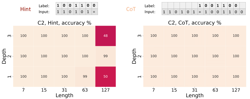
    hint: Even if the transformer has better performance in cotย setting than baseย setting, one may argue that besides the difference expressiveness, cotย setting also has a statistical advantage over base, as cotย provides more labels and thus more information about the groundtruth $f^{*}$ to the model. This motivates us to design the following loss which provides the chain of thought $c(x)$ as the labels. Here for simplicity, we assume the length of $c(x)$ is equal to $n$. 555Note such alignment is in general impossible because the CoT $c(x)$ can be even longer than $x$ itself. However, in our four settings, there exist meaningful ways to set CoT $c(x)$ as hints for earlier tokens in $x$. Formally we define $\ell_{\sf{hint}}(\theta)\triangleq\frac{1}{n}\operatorname*{\mathop{\mathbb{missing}}{E}}_{x\sim p}\sum\nolimits_{i=1}^{n}-\ln p_{\theta}(c_{i}(x)\mid{x}_{1},\dots,{x}_{i})).$

Refer to caption
Figure 3: Iterated Squaring(IS). The vocabulary ${\mathcal{V}}\triangleq\{0,1,\ldots,T-1,=,\text{\^{} 2}\}$ with $T=1000$. We randomly generate input of format $(r,p,{\text{\^{} 2},\ldots,\text{\^{} 2}},=)$ with $1\leq r,p\leq T-1$, $p$ being a prime and random number of ^2 tokens (at most $m$). The label is $f_{r,p}(n)\equiv(r^{2^{n}})\mod p$. CoT and hints are $(f_{r,p}(i))_{i=1}^{n}$. Though our construction does not exactly satisfy the technical conditions of the hardness assumption, this problem is difficult for transformers without CoT to learn, but can be perfectly expressed with CoT even with depth 1.

Performance Evaluation.

Since we train transformers using fresh sampled synthetic data each step, the training accuracy/loss is just the same as validation accuracy/loss. For baseย and hintย setting, we evaluate the accuracy of the final answer directly. For cotย setting, directly evaluating the final answer is too easy because it only measures the ability of the transformer to correctly compute the last step since CoT is given as inputs. Ideally, we should measure the answer output by transformers after auto-regressively generating $|c(x)|$ tokens. But for computational efficiency, we measure the probability that transformers can predict all tokens in the given CoT correctly. Note this probability is a lower bound of the ideal metric because there is a small possibility that transformers can answer correctly with a wrong CoT. Nevertheless, even with this slightly more difficult evaluation metric, transformers in cotย setting still optimize much faster than without CoT.

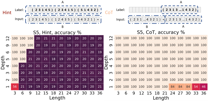
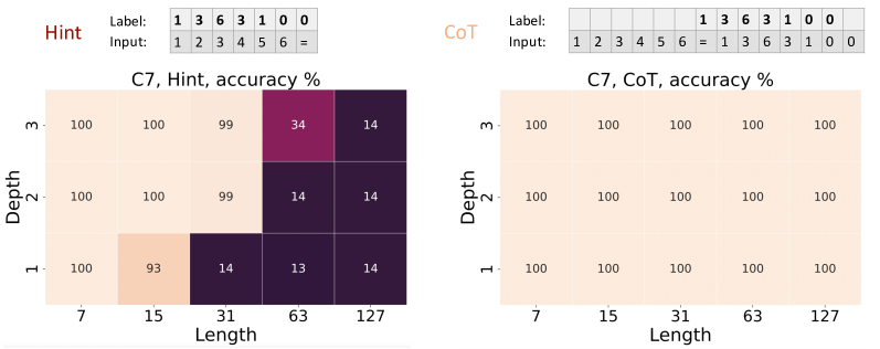
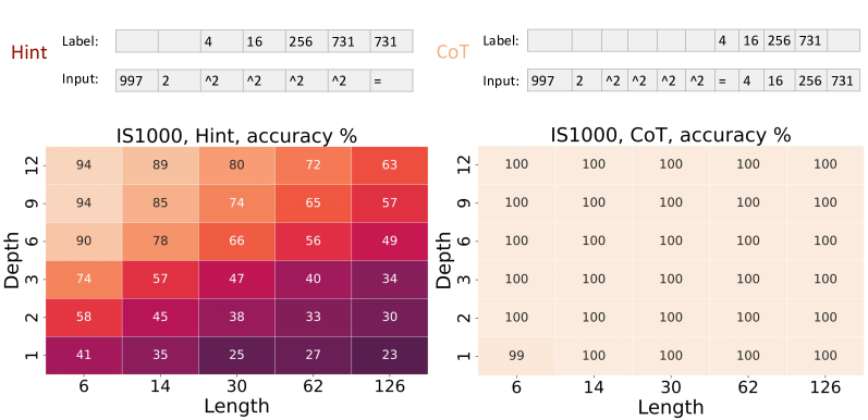
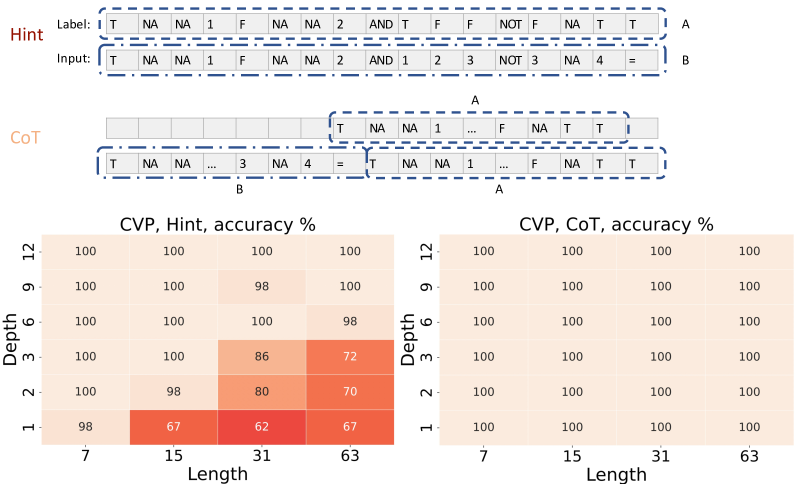
Due to space limit, we defer the details of the training and each setting to Appendixย A. Our experimental results are presented in Figuresย 2, 1, 3 andย 4.

Our Findings:

Unsurprisingly, the accuracy in hintsetting is always higher than baseย setting. Due to the space limit, we postpone all results for baseย  settings into Appendixย A. For the problems hard for parallel computation, i.e., permutation composition, iterated squaring, and circuit value problem, we find that cotย is always better than hintand base, and the improvement is huge especially when depth is small. Our experiments suggest that turning on CoT drastically improves the expressiveness of low-depth transformers on problems which are hard to be parallel computed, i.e., those inherently serial problems.

Refer to caption
Figure 4: Circuit Value Problem(CVP). Given a randomly generated circuit with $m$ gates (sorted by topological order), the vocabulary ๐’ฑ=[m]โˆช{๐–ณ๐–ฑ๐–ด๐–ค,๐–ฅ๐– ๐–ซ๐–ฒ๐–ค,๐– ๐–ญ๐–ฃ,๐–ฎ๐–ฑ,๐–ญ๐–ฎ๐–ณ,๐–ญ๐– ,=}๐’ฑdelimited-[]๐‘š๐–ณ๐–ฑ๐–ด๐–ค๐–ฅ๐– ๐–ซ๐–ฒ๐–ค๐– ๐–ญ๐–ฃ๐–ฎ๐–ฑ๐–ญ๐–ฎ๐–ณ๐–ญ๐– {\mathcal{V}}=[m]\cup\{\mathsf{TRUE},\mathsf{FALSE},\mathsf{AND},\mathsf{OR},\mathsf{NOT},\mathsf{NA},=\}. Each gate is represented by four consecutive tokens, which are gate type, two input gate ids, and the current gate id. The output is the value of the last gate $m$. CoT and hints also contain 4 tokens for each gate, which are gate type, two input gate values, and the current gate value.

5 Related Works

Despite the numerous empirical achievements, unanswered questions concerning the inner workings of neural networks capable of algorithmic reasoning. The ability of self-attention to create low-complexity circuits has been recognized (Edelman etย al., 2022; Hahn, 2020; Merrill etย al., 2021), as well as its capacity to form declarative programsย (Weiss etย al., 2021), and Turing machinesย (Dehghani etย al., 2018; Giannou etย al., 2023; Pรฉrez etย al., 2021). Moreover, it has been demonstrated that interpretable symbolic computations can be drawn from trained modelsย (Clark etย al., 2019; Tenney etย al., 2019; Vig, 2019; Wang etย al., 2022b).

Liu etย al. (2022a) is a closely related work to ours, which studies the expressiveness of low-depth transformers for semi-automata. Their setting corresponds to using only 1 step of CoT and our contribution is to show that allowing more steps of CoT enables the transformers to solve more difficult problems than semi-automata, especially those inherently serial problems, like the circuit value problem, which is $\mathsf{P}$-complete.

Constant precision versus logarithmic precision:

We note that most previous literature on the expressiveness of transformers focuses on the setting of logarithmic precision, including (Merrill & Sabharwal, 2023b; Merrill etย al., 2022, 2021; Liu etย al., 2022a), etc. One main reason as argued by Merrill & Sabharwal (2023a) is that log precision allows the transformer to use uniform attention over the rest tokens. However, recent advancements in LLMs showed that uniform attention might not be necessary towards good performance, at least for natural language tasks. For example, one of the most successful open-sourced LLM, LLAMA2 ย (Touvron etย al., 2023) takes the input of a sequence of $4096$ tokens and uses BF16 precision, which has 1 sign bit, 8 exponent bits and 7 mantissa bits (plus one extra leading bit). As a consequence, for example, $\mathsf{BF16}$ cannot express any floating-point number between $2^{8}=256$ and $2^{8}+2=258$, which makes LLAMA2 impossible to compute uniform attention over $257$ elements.

A concurrent work Feng etย al. (2023) also studies the benefit of CoT via the perspective of expressiveness, where they show with CoT, transformers can solve some specific $\mathsf{P}$-complete problem. Our result is stronger in the sense that we give a simple and clean construction for each problem in $\Ppoly$. We also note the slight difference in the settings, while we mainly focus on constant-precision transformers with $O(\log n)$ embedding size, they focus on $O(\log(n))$ precision transformers with bounded embedding size.

6 Conclusion

We study the capability of CoT for decoder-only transformers through the lens of expressiveness. We adopt the language of circuit complexity and define a new complexity class ๐–ข๐—ˆ๐–ณโ€‹[Tโ€‹(n),dโ€‹(n),sโ€‹(n),eโ€‹(n)]๐–ข๐—ˆ๐–ณ๐‘‡๐‘›๐‘‘๐‘›๐‘ ๐‘›๐‘’๐‘›\mathsf{CoT}[T(n),d(n),s(n),e(n)] which corresponds to a problem class solvable by constant-depth, constant-precision decoder-only transformers with $O(T(n))$ steps of CoT, $O(d(n))$ embedding size and floating-point numbers with $O(e(n))$ bits of exponents and Oโ€‹(sโ€‹(n))๐‘‚๐‘ ๐‘›O(s(n)) bits of significand. Our theory suggests that increasing the length of CoT can drastically make transformers more expressive. We also empirically verify our theory in four arithmetic problems. We find that for those three inherently serial problems, transformers can only express the groundtruth function by using CoT.

Acknowledgement

The authors would like to thank the support from NSF IIS 2045685. The authors also thank Wei Zhan and Lijie Chen for providing references on circuit complexity and various inspiring discussions, Cyril Zhang and Bingbin Liu for helpful discussions on Khron-Rhodes decomposition theorem, and Kaifeng Lyu for his helpful feedback.

References

  • Ba etย al. (2016) Jimmyย Lei Ba, Jamieย Ryan Kiros, and Geoffreyย E Hinton. Layer normalization. arXiv preprint arXiv:1607.06450, 2016.
  • Barrington (1986) Davidย A. Barrington. Bounded-width polynomial-size branching programs recognize exactly those languages in nc. pp.ย  1โ€“5, 1986.
  • Chandra etย al. (1983) Ashokย K Chandra, Steven Fortune, and Richard Lipton. Unbounded fan-in circuits and associative functions. In Proceedings of the fifteenth annual ACM symposium on Theory of computing, pp.ย  52โ€“60, 1983.
  • Chen etย al. (2022) Wenhu Chen, Xueguang Ma, Xinyi Wang, and Williamย W Cohen. Program of thoughts prompting: Disentangling computation from reasoning for numerical reasoning tasks. arXiv preprint arXiv:2211.12588, 2022.
  • Chiang etย al. (2023) David Chiang, Peter Cholak, and Anand Pillay. Tighter bounds on the expressivity of transformer encoders. arXiv preprint arXiv:2301.10743, 2023.
  • Chowdhery etย al. (2022) Aakanksha Chowdhery, Sharan Narang, Jacob Devlin, Maarten Bosma, Gaurav Mishra, Adam Roberts, Paul Barham, Hyungย Won Chung, Charles Sutton, Sebastian Gehrmann, etย al. Palm: Scaling language modeling with pathways. arXiv preprint arXiv:2204.02311, 2022.
  • Chung etย al. (2022) Hyungย Won Chung, Leย Hou, Shayne Longpre, Barret Zoph, Yiย Tay, William Fedus, Eric Li, Xuezhi Wang, Mostafa Dehghani, Siddhartha Brahma, etย al. Scaling instruction-finetuned language models. arXiv preprint arXiv:2210.11416, 2022.
  • Clark etย al. (2019) Kevin Clark, Urvashi Khandelwal, Omer Levy, and Christopherย D Manning. What does bert look at? an analysis of bertโ€™s attention. arXiv preprint arXiv:1906.04341, 2019.
  • Cobbe etย al. (2021) Karl Cobbe, Vineet Kosaraju, Mohammad Bavarian, Mark Chen, Heewoo Jun, Lukasz Kaiser, Matthias Plappert, Jerry Tworek, Jacob Hilton, Reiichiro Nakano, etย al. Training verifiers to solve math word problems. arXiv preprint arXiv:2110.14168, 2021.
  • Dehghani etย al. (2018) Mostafa Dehghani, Stephan Gouws, Oriol Vinyals, Jakob Uszkoreit, and ลukasz Kaiser. Universal transformers. arXiv preprint arXiv:1807.03819, 2018.
  • Drozdov etย al. (2022) Andrew Drozdov, Nathanael Schรคrli, Ekin Akyรผrek, Nathan Scales, Xinying Song, Xinyun Chen, Olivier Bousquet, and Denny Zhou. Compositional semantic parsing with large language models. arXiv preprint arXiv:2209.15003, 2022.
  • Edelman etย al. (2022) Benjaminย L Edelman, Surbhi Goel, Sham Kakade, and Cyril Zhang. Inductive biases and variable creation in self-attention mechanisms. In International Conference on Machine Learning, pp.ย  5793โ€“5831. PMLR, 2022.
  • Feng etย al. (2023) Guhao Feng, Yuntian Gu, Bohang Zhang, Haotian Ye, Diย He, and Liwei Wang. Towards revealing the mystery behind chain of thought: a theoretical perspective. arXiv preprint arXiv:2305.15408, 2023.
  • Gao etย al. (2022) Luyu Gao, Aman Madaan, Shuyan Zhou, Uri Alon, Pengfei Liu, Yiming Yang, Jamie Callan, and Graham Neubig. Pal: Program-aided language models. arXiv preprint arXiv:2211.10435, 2022.
  • Giannou etย al. (2023) Angeliki Giannou, Shashank Rajput, Jy-yong Sohn, Kangwook Lee, Jasonย D Lee, and Dimitris Papailiopoulos. Looped transformers as programmable computers. arXiv preprint arXiv:2301.13196, 2023.
  • Goldberg (1991) David Goldberg. What every computer scientist should know about floating-point arithmetic. ACM computing surveys (CSUR), 23(1):5โ€“48, 1991.
  • Google (2023) Google. Palm 2 technical report, 2023. URL https://ai.google/static/documents/palm2techreport.pdf.
  • Hahn (2020) Michael Hahn. Theoretical limitations of self-attention in neural sequence models. Transactions of the Association for Computational Linguistics, 8:156โ€“171, 2020.
  • Hao etย al. (2022) Yiding Hao, Dana Angluin, and Robert Frank. Formal language recognition by hard attention transformers: Perspectives from circuit complexity. Transactions of the Association for Computational Linguistics, 10:800โ€“810, 2022.
  • Hesse (2001) William Hesse. Division is in uniform tc0. In International Colloquium on Automata, Languages, and Programming, pp.ย  104โ€“114. Springer, 2001.
  • Huang etย al. (2022) Jiaxin Huang, Shixiangย Shane Gu, Leย Hou, Yuexin Wu, Xuezhi Wang, Hongkun Yu, and Jiawei Han. Large language models can self-improve. arXiv preprint arXiv:2210.11610, 2022.
  • IEEE (2008) IEEE. Ieee standard for floating-point arithmetic. IEEE Std 754-2008, pp.ย  1โ€“70, 2008. doi: 10.1109/IEEESTD.2008.4610935.
  • Kingma & Ba (2014) Diederikย P Kingma and Jimmy Ba. Adam: A method for stochastic optimization. arXiv preprint arXiv:1412.6980, 2014.
  • Kojima etย al. (2022) Takeshi Kojima, Shixiangย Shane Gu, Machel Reid, Yutaka Matsuo, and Yusuke Iwasawa. Large language models are zero-shot reasoners. Advances in Neural Information Processing Systems, 2022.
  • Krohn & Rhodes (1965) Kenneth Krohn and John Rhodes. Algebraic theory of machines. i. prime decomposition theorem for finite semigroups and machines. Transactions of the American Mathematical Society, 116:450โ€“464, 1965.
  • Lampinen etย al. (2022) Andrewย K Lampinen, Ishita Dasgupta, Stephanieย CY Chan, Kory Matthewson, Michaelย Henry Tessler, Antonia Creswell, Jamesย L McClelland, Janeย X Wang, and Felix Hill. Can language models learn from explanations in context? arXiv preprint arXiv:2204.02329, 2022.
  • Lewkowycz etย al. (2022) Aitor Lewkowycz, Anders Andreassen, David Dohan, Ethan Dyer, Henryk Michalewski, Vinay Ramasesh, Ambrose Slone, Cem Anil, Imanol Schlag, Theo Gutman-Solo, etย al. Solving quantitative reasoning problems with language models. Advances in Neural Information Processing Systems, 2022.
  • Liu etย al. (2022a) Bingbin Liu, Jordanย T Ash, Surbhi Goel, Akshay Krishnamurthy, and Cyril Zhang. Transformers learn shortcuts to automata. arXiv preprint arXiv:2210.10749, 2022a.
  • Liu etย al. (2022b) Yong Liu, Siqi Mai, Xiangning Chen, Cho-Jui Hsieh, and Yang You. Towards efficient and scalable sharpness-aware minimization. In Proceedings of the IEEE/CVF Conference on Computer Vision and Pattern Recognition, pp.ย  12360โ€“12370, 2022b.
  • Lombardi & Vaikuntanathan (2020) Alex Lombardi and Vinod Vaikuntanathan. Fiat-shamir for repeated squaring with applications to ppad-hardness and vdfs. In Advances in Cryptologyโ€“CRYPTO 2020: 40th Annual International Cryptology Conference, CRYPTO 2020, Santa Barbara, CA, USA, August 17โ€“21, 2020, Proceedings, Part III, pp.ย  632โ€“651. Springer, 2020.
  • Madaan & Yazdanbakhsh (2022) Aman Madaan and Amir Yazdanbakhsh. Text and patterns: For effective chain of thought, it takes two to tango. arXiv preprint arXiv:2209.07686, 2022.
  • Maler (2010) Oded Maler. On the krohn-rhodes cascaded decomposition theorem. In Time for Verification: Essays in Memory of Amir Pnueli, pp.ย  260โ€“278. Springer, 2010.
  • McNaughton & Papert (1971) Robert McNaughton and Seymourย A Papert. Counter-Free Automata (MIT research monograph no. 65). The MIT Press, 1971.
  • Merrill & Sabharwal (2023a) William Merrill and Ashish Sabharwal. A logic for expressing log-precision transformers. In Thirty-seventh Conference on Neural Information Processing Systems, 2023a.
  • Merrill & Sabharwal (2023b) William Merrill and Ashish Sabharwal. The parallelism tradeoff: Limitations of log-precision transformers. Transactions of the Association for Computational Linguistics, 11:531โ€“545, 2023b.
  • Merrill etย al. (2021) William Merrill, Yoav Goldberg, and Noahย A Smith. On the power of saturated transformers: A view from circuit complexity. arXiv preprint arXiv:2106.16213, 2021.
  • Merrill etย al. (2022) William Merrill, Ashish Sabharwal, and Noahย A Smith. Saturated transformers are constant-depth threshold circuits. Transactions of the Association for Computational Linguistics, 10:843โ€“856, 2022.
  • Nye etย al. (2021) Maxwell Nye, Andersย Johan Andreassen, Guy Gur-Ari, Henryk Michalewski, Jacob Austin, David Bieber, David Dohan, Aitor Lewkowycz, Maarten Bosma, David Luan, etย al. Show your work: Scratchpads for intermediate computation with language models. arXiv preprint arXiv:2112.00114, 2021.
  • OpenAI (2023) OpenAI. Gpt-4 technical report, 2023.
  • Pรฉrez etย al. (2019) Jorge Pรฉrez, Javier Marinkoviฤ‡, and Pablo Barcelรณ. On the turing completeness of modern neural network architectures. arXiv preprint arXiv:1901.03429, 2019.
  • Pรฉrez etย al. (2021) Jorge Pรฉrez, Pablo Barcelรณ, and Javier Marinkovic. Attention is turing complete. The Journal of Machine Learning Research, 22(1):3463โ€“3497, 2021.
  • Pippenger & Fischer (1979) Nicholas Pippenger and Michaelย J Fischer. Relations among complexity measures. Journal of the ACM (JACM), 26(2):361โ€“381, 1979.
  • Radford etย al. (2019) Alec Radford, Jeffrey Wu, Rewon Child, David Luan, Dario Amodei, and Ilya Sutskever. Language models are unsupervised multitask learners. OpenAI Blog, 1(8), 2019.
  • Rivest etย al. (1996) Ronaldย L Rivest, Adi Shamir, and Davidย A Wagner. Time-lock puzzles and timed-release crypto. 1996.
  • Shi etย al. (2023) Freda Shi, Mirac Suzgun, Markus Freitag, Xuezhi Wang, Suraj Srivats, Soroush Vosoughi, Hyungย Won Chung, Yiย Tay, Sebastian Ruder, Denny Zhou, etย al. Language models are multilingual chain-of-thought reasoners. International Conference on Machine Learning, 2023.
  • Suzgun etย al. (2022) Mirac Suzgun, Nathan Scales, Nathanael Schรคrli, Sebastian Gehrmann, Yiย Tay, Hyungย Won Chung, Aakanksha Chowdhery, Quocย V Le, Edย H Chi, Denny Zhou, etย al. Challenging big-bench tasks and whether chain-of-thought can solve them. arXiv preprint arXiv:2210.09261, 2022.
  • Tenney etย al. (2019) Ian Tenney, Dipanjan Das, and Ellie Pavlick. Bert rediscovers the classical nlp pipeline. arXiv preprint arXiv:1905.05950, 2019.
  • Touvron etย al. (2023) Hugo Touvron, Louis Martin, Kevin Stone, Peter Albert, Amjad Almahairi, Yasmine Babaei, Nikolay Bashlykov, Soumya Batra, Prajjwal Bhargava, Shruti Bhosale, etย al. Llama 2: Open foundation and fine-tuned chat models. arXiv preprint arXiv:2307.09288, 2023.
  • Vig (2019) Jesse Vig. Visualizing attention in transformer-based language representation models. arXiv preprint arXiv:1904.02679, 2019.
  • Wang etย al. (2022a) Boshi Wang, Sewon Min, Xiang Deng, Jiaming Shen, You Wu, Luke Zettlemoyer, and Huan Sun. Towards understanding chain-of-thought prompting: An empirical study of what matters. arXiv preprint arXiv:2212.10001, 2022a.
  • Wang etย al. (2022b) Kevin Wang, Alexandre Variengien, Arthur Conmy, Buck Shlegeris, and Jacob Steinhardt. Interpretability in the wild: a circuit for indirect object identification in gpt-2 small. arXiv preprint arXiv:2211.00593, 2022b.
  • Wang etย al. (2023) Xuezhi Wang, Jason Wei, Dale Schuurmans, Quoc Le, Edย Chi, Sharan Narang, Aakanksha Chowdhery, and Denny Zhou. Self-consistency improves chain of thought reasoning in language models. International Conference on Learning Representations (ICLR), 2023.
  • Wei etย al. (2022) Jason Wei, Xuezhi Wang, Dale Schuurmans, Maarten Bosma, Edย Chi, Quoc Le, and Denny Zhou. Chain of thought prompting elicits reasoning in large language models. Advances in Neural Information Processing Systems, 2022.
  • Weiss etย al. (2021) Gail Weiss, Yoav Goldberg, and Eran Yahav. Thinking like transformers. In International Conference on Machine Learning, pp.ย  11080โ€“11090. PMLR, 2021.
  • Wilson (1985) Christopherย B Wilson. Relativized circuit complexity. Journal of Computer and System Sciences, 31(2):169โ€“181, 1985.
  • Xiong etย al. (2020) Ruibin Xiong, Yunchang Yang, Diย He, Kai Zheng, Shuxin Zheng, Chen Xing, Huishuai Zhang, Yanyan Lan, Liwei Wang, and Tieyan Liu. On layer normalization in the transformer architecture. In International Conference on Machine Learning, pp.ย  10524โ€“10533. PMLR, 2020.
  • Yang etย al. (2023) Zhengyuan Yang, Linjie Li, Jianfeng Wang, Kevin Lin, Ehsan Azarnasab, Faisal Ahmed, Zicheng Liu, Ceย Liu, Michael Zeng, and Lijuan Wang. Mm-react: Prompting chatgpt for multimodal reasoning and action. arXiv preprint arXiv:2303.11381, 2023.
  • Yao (1989) Andrew Chi-Chih Yao. Circuits and local computation. pp.ย  186โ€“196, 1989.
  • Yao etย al. (2021) Shunyu Yao, Binghui Peng, Christos Papadimitriou, and Karthik Narasimhan. Self-attention networks can process bounded hierarchical languages. arXiv preprint arXiv:2105.11115, 2021.
  • Yao etย al. (2022) Shunyu Yao, Jeffrey Zhao, Dian Yu, Nan Du, Izhak Shafran, Karthik Narasimhan, and Yuan Cao. React: Synergizing reasoning and acting in language models. arXiv preprint arXiv:2210.03629, 2022.
  • Zhang etย al. (2023) Zhuosheng Zhang, Aston Zhang, Muย Li, Hai Zhao, George Karypis, and Alex Smola. Multimodal chain-of-thought reasoning in language models. arXiv preprint arXiv:2302.00923, 2023.
  • Zhou etย al. (2023) Denny Zhou, Nathanael Schรคrli, Leย Hou, Jason Wei, Nathan Scales, Xuezhi Wang, Dale Schuurmans, Olivier Bousquet, Quoc Le, and Edย Chi. Least-to-most prompting enables complex reasoning in large language models. International Conference on Learning Representations (ICLR), 2023.

Appendix A Additional Experimental Results

In this section present the experimental results for baseย setting which is omitted in the main paper and the details of training and each task. We use the nanogpt666https://github.com/karpathy/nanoGPT codebase for language modeling.

Training Details.

For all settings we use ๐– ๐–ฝ๐–บ๐—†๐– ๐–ฝ๐–บ๐—†\mathsf{Adam} with $10^{-5}$ learning rate, 00 weight decay, $\beta_{1}=0.9$, $\beta_{2}=0.95$, and gradient clipping with threshold equal to $1.0$. The total training budget is $10^{6}$ steps and we use a linear warmup in the first $2000$ steps starting from $10^{-6}$. For each step, we use a fresh sampled batch of size $64$ from population distribution. We turn off dropout and use float16. We vary the depth of the transformer for different settings while the embedding size and the number of attention heads are fixed to be $512$ and $8$ respectively.

Below we present the setting and the experimental results of each problem respectively.

Modular Addition ($C_{p}$).

Given any positive integer $p$, the vocabulary of modular addition problem is $\{0,1,\ldots,p-1,=\}$. We generate $x=(x_{1},\ldots,x_{n})$ in the following way: for each $i\in[n-1]$, we independently sample $x_{i}$ from $\{0,1,\ldots,p-1\}$ and set $x_{n}$ = โ€˜=โ€™. The label is $f^{*}(x)=\sum_{i=1}^{n-1}x_{i}\mod p$ and CoT $c(x)$ is $(\sum_{i=1}^{k}x_{i}\mod p)_{k=1}^{n-1}$. Unsurprisingly, this task is an easy task for transformers because attention can easily express the average function across different positions, and so is the sum function. Then the feedforward layers can compute the modulus of the sum and $m$. We note that the high training accuracy here is not contradictory with our Theoremย 3.1, because our sequence length is not long enough and float16 is like log-precision. This intuitive argument is elegantly extended to all solvable groups by leveraging Khron-Rhodes decomposition theorem by Liu etย al. (2022a).

Permutation Composition ($S_{p}$).

Given any $p\in\mathbb{N}^{+}$, the vocabulary of permutation composition problem is $\{1,\ldots,p,(,),=\}$. We pick $n=(p+2)m+1$ and generate $x=(x_{1},\ldots,x_{n})$ in the following way: for each $i\in[m]$, we set $x_{(p+2)(i-1)+1}$ as โ€™(โ€™, $x_{(p+2)i}$ as โ€™)โ€™ and independently sample a random permutation over $[p]$, $\sigma_{i}=(x_{(p+2)(i-1)+2},\ldots,x_{(p+2)(i-1)+p+1})$. We set $x_{n}$ to be โ€™=โ€™. Different from other settings which only have the label at one position, we have $p$ labels for this setting, which is the composition of $\sigma_{1}\circ\ldots\circ\sigma_{n}$. The CoT $c(x)$ is the partial composition from $\sigma_{1}$ to $\sigma_{n}$.

As mentioned in Sectionย 3, unless $\TC^{0}=\NC^{1}$, composition of $S_{p}$ cannot be computed by $\TC^{0}$ for any $p\geq 5$, since composition of $S_{p}$ implies the wording problem of $S_{p}$, which is $\NC^{1}$-complete under $\AC^{0}$ reductions. Since all constant-depth poly-embedding-size transformers can be simulated by $\TC^{0}$ circuitsย (Theoremย 3.2), shallow transformers are not able to solve the composition problem of $S_{p}$ for $p\geq 5$. Our experimental results in Figureย 1 matches this theoretic prediction very well.

Iterated Squaring (IS).

Iterated squaring refers to the following problem: given integers $r,n,p$, we define the iterated squaring function $f_{r,p}(n)\triangleq r^{2^{n}}\mod p$. It is often used as hardness assumptions in cryptography (Rivest etย al., 1996; Lombardi & Vaikuntanathan, 2020) that iterated squaring cannot be solved in $n-o(n)$ time even with polynomial parallel processors under certain technical conditions (e.g., $p$ is the product of two primes of a certain magnitude and there is some requirement on the order of $r$ as an element of the multiplicative group of integers modulo $p$). In other words, people conjecture there is no faster parallel algorithm than doing squaring for $n$ times.

Circuit Value Problem (CVP).

Circuit value problem is the computational problem of computing the output of a given Boolean circuit on a given input. It is complete for $\mathsf{P}$ under $\AC^{0}$-reductions. This means if one can solve CVP with constant-depth transformers (or any $\TC^{0}$ circuits), then any problem in $\mathsf{P}$ becomes solvable by $\TC^{0}$, which is widely believed to be impossible.

Refer to caption
Figure 5: Results of Modular Addition $C_{2}$.
Refer to caption
Refer to caption
Refer to caption
Figure 6: Results of baseย on Permutation Composition, Iterated Squaring, and Circuit Value Problem.
Refer to caption
Refer to caption
Figure 7: Results of Modular Addition baseย on $C_{2}$ and $C_{7}$.

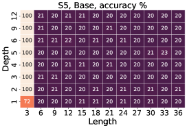
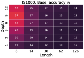
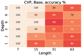
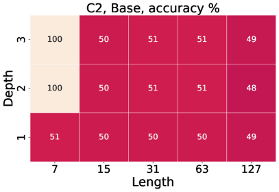
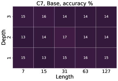
We can observe that the accuracy of baseย setting is also lower than that of hintย setting.

Appendix B Details on Finite-Precision Layers

In this section, we give the definition of the finite-precision version of different transformer layers. Recall that given sโˆˆโ„•+๐‘ superscriptโ„•s\in\mathbb{N}^{+}, the numbers representable using 2โ€‹s2๐‘ 2s-bit significand and $e$-bit exponent is ๐”ฝe,sโ‰œ{Sโ‹…2โˆ’s+Eโˆฃโˆ’22โ€‹s+1โ‰คSโ‰ค22โ€‹sโˆ’1,โˆ’2maxโก(0,eโˆ’1)โ‰คEโ‰ค2eโˆ’1โˆ’2maxโก(0,eโˆ’1),E,Sโˆˆโ„•}โ‰œsubscript๐”ฝ๐‘’๐‘ conditional-setโ‹…๐‘†superscript2๐‘ ๐ธformulae-sequencesuperscript22๐‘ 1๐‘†superscript22๐‘ 1superscript20๐‘’1๐ธsuperscript2๐‘’1superscript20๐‘’1๐ธ๐‘†โ„•\mathbb{F}_{e,s}\triangleq\{S\cdot 2^{-s+E}\mid-2^{2s}+1\leq S\leq 2^{2s}-1,-2^{\max(0,e-1)}\leq E\leq 2^{e}-1-2^{\max(0,e-1)},E,S\in\mathbb{N}\}.

Self-Attention Mechanism:

Given attention parameter ฮธ๐– ๐–ณ๐–ณ๐–ญ=(WQ,WK,WV,WO)โˆˆ๐”ฝe,sdร—dร—๐”ฝe,sdร—dร—๐”ฝe,sdร—dร—๐”ฝe,sdร—dsubscript๐œƒ๐– ๐–ณ๐–ณ๐–ญsubscript๐‘Š๐‘„subscript๐‘Š๐พsubscript๐‘Š๐‘‰subscript๐‘Š๐‘‚superscriptsubscript๐”ฝ๐‘’๐‘ ๐‘‘๐‘‘superscriptsubscript๐”ฝ๐‘’๐‘ ๐‘‘๐‘‘superscriptsubscript๐”ฝ๐‘’๐‘ ๐‘‘๐‘‘superscriptsubscript๐”ฝ๐‘’๐‘ ๐‘‘๐‘‘\theta_{\mathsf{ATTN}}=(W_{Q},W_{K},W_{V},W_{O})\in\mathbb{F}_{e,s}^{d\times d}\times\mathbb{F}_{e,s}^{d\times d}\times\mathbb{F}_{e,s}^{d\times d}\times\mathbb{F}_{e,s}^{d\times d}, we define the self-attention layer with causal mask for decoder-only transformer in Algorithmย 3.

Algorithm 3 Finite-Precision Causal Self-Attention, ๐– ๐–ณ๐–ณ๐–ญ๐– ๐–ณ๐–ณ๐–ญ\mathsf{ATTN}
1:Integer sโˆˆโ„•+๐‘ superscriptโ„•s\in\mathbb{N}^{+}, $e\in\mathbb{N}$, Parameter ฮธ๐– ๐–ณ๐–ณ๐–ญ=(WQ,WK,WV,WO)subscript๐œƒ๐– ๐–ณ๐–ณ๐–ญsubscript๐‘Š๐‘„subscript๐‘Š๐พsubscript๐‘Š๐‘‰subscript๐‘Š๐‘‚\theta_{\mathsf{ATTN}}=(W_{Q},W_{K},W_{V},W_{O}), Input embedding h=(h1,โ€ฆ,hn)โˆˆ๐”ฝe,snโ€‹dโ„Žsubscriptโ„Ž1โ€ฆsubscriptโ„Ž๐‘›superscriptsubscript๐”ฝ๐‘’๐‘ ๐‘›๐‘‘h=(h_{1},\ldots,h_{n})\in\mathbb{F}_{e,s}^{nd}.
2:Output embedding hโ€ฒ=(h1โ€ฒ,โ€ฆ,hnโ€ฒ)โ‰œ๐– ๐–ณ๐–ณ๐–ญฮธ๐– ๐–ณ๐–ณ๐–ญโ€‹(h1,โ€ฆ,hn)superscriptโ„Žโ€ฒsubscriptsuperscriptโ„Žโ€ฒ1โ€ฆsubscriptsuperscriptโ„Žโ€ฒ๐‘›โ‰œsubscript๐– ๐–ณ๐–ณ๐–ญsubscript๐œƒ๐– ๐–ณ๐–ณ๐–ญsubscriptโ„Ž1โ€ฆsubscriptโ„Ž๐‘›h^{\prime}=(h^{\prime}_{1},\ldots,h^{\prime}_{n})\triangleq\mathsf{ATTN}_{\theta_{\mathsf{ATTN}}}(h_{1},\ldots,h_{n}).
3:qiโ‰œWQร—e,shi,kiโ‰œWKร—e,shi,viโ‰œWVร—e,shi,โˆ€iโˆˆ[n]formulae-sequenceโ‰œsubscript๐‘ž๐‘–subscript๐‘’๐‘ subscript๐‘Š๐‘„subscriptโ„Ž๐‘–formulae-sequenceโ‰œsubscript๐‘˜๐‘–subscript๐‘’๐‘ subscript๐‘Š๐พsubscriptโ„Ž๐‘–formulae-sequenceโ‰œsubscript๐‘ฃ๐‘–subscript๐‘’๐‘ subscript๐‘Š๐‘‰subscriptโ„Ž๐‘–for-all๐‘–delimited-[]๐‘›q_{i}\triangleq W_{Q}\times_{e,s}h_{i},k_{i}\triangleq W_{K}\times_{e,s}h_{i},v_{i}\triangleq W_{V}\times_{e,s}h_{i},\forall i\in[n]
4:siโ‰œsoftmaxe,sโ€‹(โŸจqi,k1โŸฉe,s,โ€ฆ,โŸจqi,kiโŸฉe,s)โˆฅ(0,โ€ฆ,0)โ‰œsubscript๐‘ ๐‘–conditionalsubscriptsoftmax๐‘’๐‘ subscriptsubscript๐‘ž๐‘–subscript๐‘˜1๐‘’๐‘ โ€ฆsubscriptsubscript๐‘ž๐‘–subscript๐‘˜๐‘–๐‘’๐‘ 0โ€ฆ0s_{i}\triangleq\mathrm{softmax}_{e,s}(\left\langle q_{i},k_{1}\right\rangle_{e,s},\ldots,\left\langle q_{i},k_{i}\right\rangle_{e,s})\|(0,\ldots,0). $\triangleright$ $n-i$โ€™s 0; Mask for Causal Attention;
5:hiโ€ฒโ‰œWOร—e,s๐—Œ๐—Ž๐—†e,sโ€‹([v1,โ€ฆ,vn]ร—e,ssi)โ‰œsubscriptsuperscriptโ„Žโ€ฒ๐‘–subscript๐‘’๐‘ subscript๐‘Š๐‘‚subscript๐—Œ๐—Ž๐—†๐‘’๐‘ subscript๐‘’๐‘ subscript๐‘ฃ1โ€ฆsubscript๐‘ฃ๐‘›subscript๐‘ ๐‘–h^{\prime}_{i}\triangleq W_{O}\times_{e,s}\mathsf{sum}_{e,s}([v_{1},\ldots,v_{n}]\times_{e,s}s_{i}).

Feed-Forward Network:

Given sโˆˆโ„•+๐‘ superscriptโ„•s\in\mathbb{N}^{+}, $e\in\mathbb{N}$, and the parameter of fully-connected feedforward network layer ฮธ๐–ฅ๐–ฅ=(W1,b1,W2,b2)โˆˆ๐”ฝe,sdร—dร—๐”ฝe,sdร—๐”ฝe,sdร—dร—๐”ฝe,sdsubscript๐œƒ๐–ฅ๐–ฅsubscript๐‘Š1subscript๐‘1subscript๐‘Š2subscript๐‘2superscriptsubscript๐”ฝ๐‘’๐‘ ๐‘‘๐‘‘superscriptsubscript๐”ฝ๐‘’๐‘ ๐‘‘superscriptsubscript๐”ฝ๐‘’๐‘ ๐‘‘๐‘‘superscriptsubscript๐”ฝ๐‘’๐‘ ๐‘‘\theta_{\mathsf{FF}}=(W_{1},b_{1},W_{2},b_{2})\in\mathbb{F}_{e,s}^{d\times d}\times\mathbb{F}_{e,s}^{d}\times\mathbb{F}_{e,s}^{d\times d}\times\mathbb{F}_{e,s}^{d}, we define the fully-connected feedforward layer ๐–ฅ๐–ฅฮธ๐–ฅ๐–ฅ:๐”ฝe,sdโ†’๐”ฝe,sd:subscript๐–ฅ๐–ฅsubscript๐œƒ๐–ฅ๐–ฅโ†’superscriptsubscript๐”ฝ๐‘’๐‘ ๐‘‘superscriptsubscript๐”ฝ๐‘’๐‘ ๐‘‘\mathsf{FF}_{\theta_{\mathsf{FF}}}:\mathbb{F}_{e,s}^{d}\to\mathbb{F}_{e,s}^{d} as ๐–ฅ๐–ฅฮธ๐–ฅ๐–ฅโ€‹(h)โ‰œ[W2ร—e,s๐—‹๐–พ๐—…๐—Žโ€‹([W1ร—e,sh+b1]e,s)+b2]e,sโ‰œsubscript๐–ฅ๐–ฅsubscript๐œƒ๐–ฅ๐–ฅโ„Žsubscriptdelimited-[]subscript๐‘’๐‘ subscript๐‘Š2๐—‹๐–พ๐—…๐—Žsubscriptdelimited-[]subscript๐‘’๐‘ subscript๐‘Š1โ„Žsubscript๐‘1๐‘’๐‘ subscript๐‘2๐‘’๐‘ \mathsf{FF}_{\theta_{\mathsf{FF}}}(h)\triangleq\left[W_{2}\times_{e,s}\mathsf{relu}(\left[W_{1}\times_{e,s}h+b_{1}\right]_{e,s})+b_{2}\right]_{e,s}.

Token Embedding:

Given sโˆˆโ„•+๐‘ superscriptโ„•s\in\mathbb{N}^{+}, $e\in\mathbb{N}$, and the parameter of token embedding layer ฮธ๐–ณ๐–คโˆˆ๐”ฝe,sdร—|๐’ฑ|subscript๐œƒ๐–ณ๐–คsuperscriptsubscript๐”ฝ๐‘’๐‘ ๐‘‘๐’ฑ\theta_{\mathsf{TE}}\in\mathbb{F}_{e,s}^{d\times|{\mathcal{V}}|}, we define the token embedding layer by viewing $\theta_{\mathsf{TE}}$ as a mapping from ${\mathcal{V}}$ to $\mathbb{R}^{d}$, that is, for all $x\in{\mathcal{V}}$, the token embedding is $\theta_{\mathsf{TE}}(x)$.

Position Encoding:

Given sโˆˆโ„•+๐‘ superscriptโ„•s\in\mathbb{N}^{+}, $e\in\mathbb{N}$, and the parameter of position encoding layer ฮธ๐–ฏ๐–คโˆˆ๐”ฝe,sdร—nmaxsubscript๐œƒ๐–ฏ๐–คsuperscriptsubscript๐”ฝ๐‘’๐‘ ๐‘‘subscript๐‘›\theta_{\mathsf{PE}}\in\mathbb{F}_{e,s}^{d\times n_{\max}}, we define the token embedding layer by viewing $\theta_{\mathsf{PE}}$ as a mapping from $[n_{\max}]$ to $\mathbb{R}^{d}$ that is, for all $n\in[n_{\max}]$, the position embedding is as $\theta_{\mathsf{PE}}(n)$.

Output Layer:

Given sโˆˆโ„•+๐‘ superscriptโ„•s\in\mathbb{N}^{+}, $e\in\mathbb{N}$, and the parameter of output layer ฮธ๐–ฎ๐–ด๐–ณ๐–ฏ๐–ด๐–ณโˆˆ๐”ฝe,s|๐’ฑ|ร—dsubscript๐œƒ๐–ฎ๐–ด๐–ณ๐–ฏ๐–ด๐–ณsuperscriptsubscript๐”ฝ๐‘’๐‘ ๐’ฑ๐‘‘\theta_{\mathsf{OUTPUT}}\in\mathbb{F}_{e,s}^{|{\mathcal{V}}|\times d}, we define the output layer ๐–ฎ๐–ด๐–ณ๐–ฏ๐–ด๐–ณฮธ๐–ฎ๐–ด๐–ณ๐–ฏ๐–ด๐–ณ:๐”ฝe,sdโ†’๐’ฑ:subscript๐–ฎ๐–ด๐–ณ๐–ฏ๐–ด๐–ณsubscript๐œƒ๐–ฎ๐–ด๐–ณ๐–ฏ๐–ด๐–ณโ†’superscriptsubscript๐”ฝ๐‘’๐‘ ๐‘‘๐’ฑ\mathsf{OUTPUT}_{\theta_{\mathsf{OUTPUT}}}:\mathbb{F}_{e,s}^{d}\to{\mathcal{V}} as ๐–ฎ๐–ด๐–ณ๐–ฏ๐–ด๐–ณฮธ๐–ฎ๐–ด๐–ณ๐–ฏ๐–ด๐–ณโ€‹(h)โ‰œsoftmaxe,sโ€‹(ฮธ๐–ฎ๐–ด๐–ณ๐–ฏ๐–ด๐–ณร—e,sh)โ‰œsubscript๐–ฎ๐–ด๐–ณ๐–ฏ๐–ด๐–ณsubscript๐œƒ๐–ฎ๐–ด๐–ณ๐–ฏ๐–ด๐–ณโ„Žsubscriptsoftmax๐‘’๐‘ subscript๐‘’๐‘ subscript๐œƒ๐–ฎ๐–ด๐–ณ๐–ฏ๐–ด๐–ณโ„Ž\mathsf{OUTPUT}_{\theta_{\mathsf{OUTPUT}}}(h)\triangleq\mathrm{softmax}_{e,s}(\theta_{\mathsf{OUTPUT}}\times_{e,s}h) for all hโˆˆ๐”ฝe,sdโ„Žsuperscriptsubscript๐”ฝ๐‘’๐‘ ๐‘‘h\in\mathbb{F}_{e,s}^{d}.

Finally, we define finite-precision decoder-only transformers below.

Algorithm 4 Finite-precision Decoder-only Transformer, $\mathsf{TF}_{\theta}$ and $p_{\theta}$
1:Integer sโˆˆโ„•+๐‘ superscriptโ„•s\in\mathbb{N}^{+}, $e\in\mathbb{N}$. Transformer parameter ฮธ=(ฮธ๐–ฏ๐–ค,ฮธ๐–ณ๐–ค,ฮธ๐–ฎ๐–ด๐–ณ๐–ฏ๐–ด๐–ณ,{ฮธ๐– ๐–ณ๐–ณ๐–ญ(l),ฮธ๐–ฅ๐–ฅ(l)}l=0Lโˆ’1)๐œƒsubscript๐œƒ๐–ฏ๐–คsubscript๐œƒ๐–ณ๐–คsubscript๐œƒ๐–ฎ๐–ด๐–ณ๐–ฏ๐–ด๐–ณsuperscriptsubscriptsubscriptsuperscript๐œƒ๐‘™๐– ๐–ณ๐–ณ๐–ญsubscriptsuperscript๐œƒ๐‘™๐–ฅ๐–ฅ๐‘™0๐ฟ1\theta=(\theta_{\mathsf{PE}},\theta_{\mathsf{TE}},\theta_{\mathsf{OUTPUT}},\{\theta^{(l)}_{\mathsf{ATTN}},\theta^{(l)}_{\mathsf{FF}}\}_{l=0}^{L-1}) with 2โ€‹s2๐‘ 2s-bit precision and $e$-bit exponent. Input tokens $x=(x_{1},\ldots,x_{n})\in{\mathcal{V}}^{n}$.
2:Output distribution $p_{\theta}(\cdot\mid x_{1},\ldots,x_{i})$ for all $i\in[n]$ and output token $\mathsf{TF}_{\theta}(x)$.
3:hi(0)โ‰œ[๐–ณ๐–คโ€‹(xi)+๐–ฏ๐–คโ€‹(i)]e,s,โˆ€iโˆˆ[n]formulae-sequenceโ‰œsubscriptsuperscriptโ„Ž0๐‘–subscriptdelimited-[]๐–ณ๐–คsubscript๐‘ฅ๐‘–๐–ฏ๐–ค๐‘–๐‘’๐‘ for-all๐‘–delimited-[]๐‘›h^{(0)}_{i}\triangleq\left[\mathsf{TE}(x_{i})+\mathsf{PE}(i)\right]_{e,s},\forall i\in[n]
4:forย l=0,โ€ฆ,Lโˆ’1๐‘™0โ€ฆ๐ฟ1l=0,\ldots,L-1ย do
5:ย ย ย ย ย (h1(l+0.5),โ€ฆ,hn(l+0.5))โ‰œ[(h1(l),โ€ฆ,hn(l))+๐– ๐–ณ๐–ณ๐–ญฮธ๐– ๐–ณ๐–ณ๐–ญ(l)โ€‹(h1(l),โ€ฆ,hn(l))]e,sโ‰œsubscriptsuperscriptโ„Ž๐‘™0.51โ€ฆsubscriptsuperscriptโ„Ž๐‘™0.5๐‘›subscriptdelimited-[]subscriptsuperscriptโ„Ž๐‘™1โ€ฆsubscriptsuperscriptโ„Ž๐‘™๐‘›subscript๐– ๐–ณ๐–ณ๐–ญsubscriptsuperscript๐œƒ๐‘™๐– ๐–ณ๐–ณ๐–ญsubscriptsuperscriptโ„Ž๐‘™1โ€ฆsubscriptsuperscriptโ„Ž๐‘™๐‘›๐‘’๐‘ (h^{(l+0.5)}_{1},\ldots,h^{(l+0.5)}_{n})\triangleq\left[(h^{(l)}_{1},\ldots,h^{(l)}_{n})+\mathsf{ATTN}_{\theta^{(l)}_{\mathsf{ATTN}}}(h^{(l)}_{1},\ldots,h^{(l)}_{n})\right]_{e,s}
6:ย ย ย ย ย hi(l+1)โ‰œ[hi(l+0.5)+๐–ฅ๐–ฅฮธ๐–ฅ๐–ฅ(l)โ€‹(hi(l+0.5))]e,sโ‰œsubscriptsuperscriptโ„Ž๐‘™1๐‘–subscriptdelimited-[]subscriptsuperscriptโ„Ž๐‘™0.5๐‘–subscript๐–ฅ๐–ฅsubscriptsuperscript๐œƒ๐‘™๐–ฅ๐–ฅsubscriptsuperscriptโ„Ž๐‘™0.5๐‘–๐‘’๐‘ h^{(l+1)}_{i}\triangleq\left[h^{(l+0.5)}_{i}+\mathsf{FF}_{\theta^{(l)}_{\mathsf{FF}}}(h^{(l+0.5)}_{i})\right]_{e,s}, $\forall i\in[n]$
7:endย for
8:$p_{\theta}(\cdot\mid x_{1},\ldots,x_{i})\triangleq\left[\mathsf{OUTPUT}_{\theta_{\mathsf{OUTPUT}}}(h^{(L)}_{i})\right]_{e,s},\forall i\in[n]$
9:$\mathsf{TF}_{\theta}(x)\triangleq\operatorname*{arg\,max}_{x}p_{\theta}(x\mid x_{1},\ldots,x_{n})$.

Appendix C Preliminary of Automata and Krohn-Rhodes Decomposition Theorem

In this section we recap the basic notations and definitions for automata theory and Krohn-Rhodes Decomposition Theoremย (Krohn & Rhodes, 1965), following the notation and presentation of Maler (2010).

Definition C.1 (Automaton).

A deterministic automaton is triple ${\mathcal{A}}=(\Sigma,Q,\delta)$ where $\Sigma$ is a finite set of symbols called the input alphabet, $Q$ is a finite set of states and $\delta:Q\times\Sigma\to Q$ is the transition function.

The transition function can be lifted naturally to input sequences, by letting $\delta(q,w\sigma)\triangleq\delta(\delta(q,w),\sigma)$ for all $w\in\Sigma^{*}$ recursively.

An automaton can be made an acceptor by choosing an initial state $q_{0}\in Q$ and a set of accepting states $F\subseteq Q$. As such it accepts/recognizes a set of sequences, also known as a language, defined as ${\mathcal{L}}(A,q_{0},F)=\{w\in\Sigma^{*}:\delta(q_{0},w)\in F\}$. Kleeneโ€™s Theorem states that the class of languages recognizable by finite automata coincides with the regular languages.

Definition C.2 (Automaton Homomorphism).

A surjection $\phi:Q\to Q_{0}$ is an automaton homomorphism from ${\mathcal{A}}=(\Sigma,Q,\delta)$ to ${\mathcal{A}}_{0}=(\Sigma,Q_{0},\delta_{0})$ if for every $q\in Q,\sigma\in\Sigma,\phi(\delta(q,\sigma))=\delta_{0}(\phi(q),\sigma)$. In such a case we say that ${\mathcal{A}}_{0}$ is homomorphic to ${\mathcal{A}}$ and denote it by ${\mathcal{A}}_{0}\leq_{\phi}{\mathcal{A}}$. When $\phi$ is a bijection, ${\mathcal{A}}$ and ${\mathcal{A}}_{0}$ are said to be isomorphic.

The conceptual significance of Automaton Homomorphism is that, if we can simulate any ${\mathcal{A}}$ and ${\mathcal{A}}_{0}\leq_{\phi}{\mathcal{A}}$, we can โ€˜almostโ€™ simulate ${\mathcal{A}}_{0}$ as well, in the sense of following lemma:

Lemma C.1.

For any two automata ${\mathcal{A}}=(\Sigma,Q,\delta),{\mathcal{A}}_{0}=(\Sigma,Q_{0},\delta_{0})$ satisfying that ${\mathcal{A}}_{0}\leq_{\phi}{\mathcal{A}}$ for some function $\phi$, for any $F_{0}\subseteq Q$, $q_{0}\in Q$, $\phi(q)=q_{0}$, it holds that ${\mathcal{L}}({\mathcal{A}}_{0},q_{0},F_{0})={\mathcal{L}}({\mathcal{A}},q,\phi^{-1}(F_{0}))$.

Proof of Lemmaย C.1.

We claim for any $w\in\Sigma^{*}$, it holds that $\phi(\delta(q,w))=\delta(\phi(q),w)$. This claim holds by definition of automaton homomorphism for all $|w|\leq 1$. suppose the claim already holds for all $w$ no longer than $n$ for some $n$, for any $w^{\prime}=w\sigma$ with $|w|=n$ and $\sigma\in\Sigma$, it holds that $\phi(\delta(q,w^{\prime}))=\phi(\delta(\delta(q,w),\sigma))=\delta(\phi(\delta(q,w)),\sigma)=\delta(\delta(\phi(q),w),\sigma)=\delta(\phi(q),w^{\prime})$. Therefore $\delta_{0}(q_{0},w)\in F_{0}\iff\delta_{0}(\phi(q),w)\in F_{0}\iff\phi(\delta(q,w))\in F_{0}\iff\delta(q,w)\in\phi^{-1}(F_{0})$. Thus we conclude that ${\mathcal{L}}({\mathcal{A}}_{0},q_{0},F_{0})=\{w\in\Sigma^{*}\mid\delta(q_{0},w)\in F_{0}\}=\{w\in\Sigma^{*}\mid\delta(q,w)\in\phi^{-1}(F_{0})\}={\mathcal{L}}({\mathcal{A}},q,\phi^{-1}(F_{0}))$. โˆŽ

Definition C.3 (Semigroups, Monoids and Groups).

A Semigroup is a pair $(S,\cdot)$ where $S$ is a set and $\cdot$ is a binary associative operation (โ€œmultiplicationโ€) from $S\times S$ to $S$. A Monoid $(S,\cdot,1)$ is a semigroup admitting an identity element $1$ such that sโ‹…1=1โ€‹โ‹ฏ=sโ‹…๐‘ 11โ‹ฏ๐‘ s\cdot 1=1\cdots=s for every sโˆˆS๐‘ ๐‘†s\in S. A group is a monoid such that for every sโˆˆS๐‘ ๐‘†s\in S there exists an element sโˆ’1โˆˆSsuperscript๐‘ 1๐‘†s^{-1}\in S (an inverse) such that sโ‹…sโˆ’1=1โ‹…๐‘ superscript๐‘ 11s\cdot s^{-1}=1.

Definition C.4 (Semigroup Homomorphisms).

A surjective function $\phi:S\to S_{0}$ is a semigroup homomorphism from $(S,\cdot)$ to $(S_{0},\ast)$ if for every s1,s2โˆˆS,ฯ•โ€‹(s1โ‹…s2)=ฯ•โ€‹(s1)โˆ—ฯ•โ€‹(s2)formulae-sequencesubscript๐‘ 1subscript๐‘ 2๐‘†italic-ฯ•โ‹…subscript๐‘ 1subscript๐‘ 2โˆ—italic-ฯ•subscript๐‘ 1italic-ฯ•subscript๐‘ 2s_{1},s_{2}\in S,\phi(s_{1}\cdot s_{2})=\phi(s_{1})\ast\phi(s_{2}). In such a case we say that $S_{0}$ is homomorphic to $S$ and denote it by $S_{0}\leq_{\phi}S$. Two mutually homomorphic semigroups are said to be isomorphic.

Definition C.5 (Transformation Semigroup).

The transformation semigroup of an automata ${\mathcal{A}}=(\Sigma,Q,\delta)$ is the semigroup generated by $\{\delta(\cdot,\sigma):Q\to Q\mid\sigma\in\Sigma\}$.

C.1 The Krohn-Rhodes Decomposition Theorem

Below we give the definition of the cascade product of two automata, which is a central concept used in Krohn-Rhodes Decomposition Theorem for automata.

Definition C.6 (Cascade Product).

Let ${\mathcal{B}}_{1}=(\Sigma,Q_{1},\delta_{1})$ and ${\mathcal{B}}_{2}=(Q_{1}\times\Sigma,Q_{2},\delta_{2})$ be two automata. The cascade product ${\mathcal{B}}_{1}\circ{\mathcal{B}}_{2}$ is the automaton $C=(\Sigma,Q_{1}\times Q_{2},\overline{\delta})$ where

$$\overline{\delta}((q_{1},q_{2}),\sigma)\triangleq(\delta_{1}(q_{1},\sigma),\delta_{2}(q_{2},(q_{1},\sigma))).$$

The cascade product of more than two automata is defined as ${\mathcal{B}}_{1}\circ{\mathcal{B}}_{2}\circ\cdots\circ{\mathcal{B}}_{k}=(\cdots(({\mathcal{B}}_{1}\circ{\mathcal{B}}_{2})\circ B_{3}\cdots)\circ{\mathcal{B}}_{k}$.

Definition C.7 (Permutation-Reset Automata).

A automaton ${\mathcal{A}}=(\Sigma,Q,\delta)$ is a permutation-reset automaton if for every letter $\sigma\in\Sigma$, $\sigma$ is either a permutation or reset. If the only permutations are identities, we call it a reset automaton.

Theorem C.2 (Krohn-Rhodes; cf. Maler (2010)).

For every automaton A there exists a cascade ${\mathcal{C}}={\mathcal{B}}_{1}\circ{\mathcal{B}}_{2}\circ\cdot\cdot\cdot\circ{\mathcal{B}}_{k}$ such that:

  1. 1.

    Each ${\mathcal{B}}_{i}$ is a permutation-reset automaton;

  2. 2.

    There is a homomorphism $\phi$ from ${\mathcal{C}}$ to ${\mathcal{A}}$;

  3. 3.

    Any permutation group in some ${\mathcal{B}}_{i}$ is homomorphic to a subgroup of the transformation semigroup of ${\mathcal{A}}$.

The pair $({\mathcal{C}},\phi)$ is called a cascaded decomposition of ${\mathcal{A}}$.

C.2 Counter-free Automata

Next we introduce a key concept used in the proof of Theoremย D.1 (and thus Theoremย 3.1) โ€“ Counter-free Automaton.

Definition C.8 (Counter-free Automaton, (McNaughton & Papert, 1971)).

An automaton is counter-free if no word $w\in\Sigma^{*}$ induces a permutation other than identity on any subset of $Q$.

A subclass of the regular languages is the class of star-free sets defined as:

Definition C.9 (Star-Free regular languages).

The class of star-free regular languages over $\Sigma$ is the smallest class containing $\Sigma^{\ast}$ and the sets of the form $\{\sigma\}$ where $\sigma\in\sigma\cup\{\epsilon\}$, which is closed under finitely many applications of concatenation and Boolean operations including union, intersection, and complementation.

It is well-known that languages recognized by counter-free automata have the following equivalent characterizations.

Theorem C.3 (McNaughton & Papert (1971)).

Suppose $L$ is a regular language not containing the empty string. Then the following are equivalent:

  1. 1.

    $L$ is star-free;

  2. 2.

    $L$ is accepted by a counter-free automata.

  3. 3.

    $L$ is non-counting, i.e., there is an $n\in\mathbb{N}$ so that for all $x$, $y$, and $z$ and all $m\geq n$, $xy^{m}z\in L\iff xy^{m+1}z\in L$.

Counter-free property of an automaton can also be characterized via its transformation semigroup by Lemmaย C.4, whose proof is straightforward and skipped.

Lemma C.4.

An automaton is counter-free if and only if the transformation semigroup of the automaton is group-free, i.e., it has no non-trivial subgroups. A semigroup $(S,\cdot)$ is group-free if and only if it is aperiodic, i.e., for all sโˆˆS๐‘ ๐‘†s\in S, there exists $k\in\mathbb{N}$, sk=sk+1superscript๐‘ ๐‘˜superscript๐‘ ๐‘˜1s^{k}=s^{k+1}.

Thus Theoremย C.5 holds as a corollary of Theoremย C.2.

Theorem C.5 (Corollary of Theoremย C.2).

For every counter-free automaton ${\mathcal{A}}$ there exists a cascade ${\mathcal{C}}={\mathcal{B}}_{1}\circ{\mathcal{B}}_{2}\circ\cdot\cdot\cdot\circ{\mathcal{B}}_{k}$ such that each ${\mathcal{B}}_{i}$ is a reset automaton and there is a homomorphism $\phi$ from ${\mathcal{C}}$ to ${\mathcal{A}}$.

Using Theoremย C.5 the following theorem connects the counter-free automata to constant-depth poly-size circuits with unbounded fan-in. The high-level proof idea is that any reset automaton can be simulated using constantly many depth and any counter-free automaton can be decomposed into the cascade product of a finite number of reset automaton.

Theorem C.6.

[Theorem 2.6, Chandra etย al. (1983)] Suppose ${\mathcal{A}}=(\Sigma,Q,\delta)$ is an counter-free automaton. Then there is a circuit of size $O(n^{3})$ with unbounded fan-in and constant depth that simulates $\delta(q,w)$ for any $q\in Q$ and $w\in\Sigma^{*}$ satisfying $|w|=n$, where $O(\cdot)$ hides constants depending on the automaton.

Appendix D Proofs for Expressiveness Upper Bounds (Sectionย 3.3)

The main technical theorems we will prove in this section are Theoremsย D.1 andย D.2. Their proofs can be found in Sectionsย D.1 andย D.2 respectively.

Recall ฯˆe,s:๐”ฝe,sโ†’{0,1}e+2โ€‹s+1:subscript๐œ“๐‘’๐‘ โ†’subscript๐”ฝ๐‘’๐‘ superscript01๐‘’2๐‘ 1\psi_{e,s}:\mathbb{F}_{e,s}\to\{0,1\}^{e+2s+1} is the binary representation of floating point with $e$-bit exponent and 2โ€‹s2๐‘ 2s-bit precision.

Theorem D.1.

For any fixed eโˆˆโ„•,sโˆˆโ„•+formulae-sequence๐‘’โ„•๐‘ superscriptโ„•e\in\mathbb{N},s\in\mathbb{N}^{+}, ๐—Œ๐—Ž๐—†e,s:(๐”ฝe,s)nโ†’๐”ฝe,s:subscript๐—Œ๐—Ž๐—†๐‘’๐‘ โ†’superscriptsubscript๐”ฝ๐‘’๐‘ ๐‘›subscript๐”ฝ๐‘’๐‘ \mathsf{sum}_{e,s}:(\mathbb{F}_{e,s})^{n}\to\mathbb{F}_{e,s} has $\AC^{0}$ circuits.

In detail, there is a family of $\AC^{0}$ circuits $\{C_{n}\}$ such that for all x1,โ€ฆ,xnโˆˆ๐”ฝe,ssubscript๐‘ฅ1โ€ฆsubscript๐‘ฅ๐‘›subscript๐”ฝ๐‘’๐‘ x_{1},\ldots,x_{n}\in\mathbb{F}_{e,s}, it holds that

Cnโ€‹(ฯˆe,sโ€‹(x1)โ€‹โ€–โ€ฆโ€–โ€‹ฯˆe,sโ€‹(xn))=ฯˆe,sโ€‹(๐—Œ๐—Ž๐—†e,sโ€‹(x1,โ€ฆ,xn))subscript๐ถ๐‘›subscript๐œ“๐‘’๐‘ subscript๐‘ฅ1normโ€ฆsubscript๐œ“๐‘’๐‘ subscript๐‘ฅ๐‘›subscript๐œ“๐‘’๐‘ subscript๐—Œ๐—Ž๐—†๐‘’๐‘ subscript๐‘ฅ1โ€ฆsubscript๐‘ฅ๐‘›C_{n}(\psi_{e,s}(x_{1})\|\dots\|\psi_{e,s}(x_{n}))=\psi_{e,s}(\mathsf{sum}_{e,s}(x_{1},\dots,x_{n})) (2)
Theorem D.2.

For sโ€‹(n)=Oโ€‹(\polyโ€‹(n))๐‘ ๐‘›๐‘‚\poly๐‘›s(n)=O(\poly(n)), ๐—Œ๐—Ž๐—†0,sโ€‹(n):(๐”ฝ0,sโ€‹(n))nโ†’๐”ฝ0,sโ€‹(n):subscript๐—Œ๐—Ž๐—†0๐‘ ๐‘›โ†’superscriptsubscript๐”ฝ0๐‘ ๐‘›๐‘›subscript๐”ฝ0๐‘ ๐‘›\mathsf{sum}_{0,s(n)}:(\mathbb{F}_{0,s(n)})^{n}\to\mathbb{F}_{0,s(n)} has $\TC^{0}$ circuits.

In detail, there is a family of $\TC^{0}$ circuits $\{C_{n}\}$ such that for all x1,โ€ฆ,xnโˆˆ๐”ฝ0,sโ€‹(n)subscript๐‘ฅ1โ€ฆsubscript๐‘ฅ๐‘›subscript๐”ฝ0๐‘ ๐‘›x_{1},\ldots,x_{n}\in\mathbb{F}_{0,s(n)}, it holds that

Cnโ€‹(ฯˆ0,sโ€‹(n)โ€‹(x1)โ€‹โ€–โ€ฆโ€–โ€‹ฯˆ0,sโ€‹(n)โ€‹(xn))=ฯˆ0,sโ€‹(n)โ€‹(๐—Œ๐—Ž๐—†e,sโ€‹(x1,โ€ฆ,xn))subscript๐ถ๐‘›subscript๐œ“0๐‘ ๐‘›subscript๐‘ฅ1normโ€ฆsubscript๐œ“0๐‘ ๐‘›subscript๐‘ฅ๐‘›subscript๐œ“0๐‘ ๐‘›subscript๐—Œ๐—Ž๐—†๐‘’๐‘ subscript๐‘ฅ1โ€ฆsubscript๐‘ฅ๐‘›C_{n}(\psi_{0,s(n)}(x_{1})\|\dots\|\psi_{0,s(n)}(x_{n}))=\psi_{0,s(n)}(\mathsf{sum}_{e,s}(x_{1},\dots,x_{n})) (3)

With Theoremsย D.1 andย D.2 ready, Theoremsย 3.1 andย 3.2 are standard (e.g., see proof of Theorem 4 in Liu etย al. (2022a)) and thus are omitted.

D.1 Proofs for Theoremย D.1

Definition D.1 (Total Order).

A total order $\leq$ on some set $X$ is a binary relationship satisfying that for all $a,b,c\in X$:

  1. 1.

    $a\leq a$ (reflexive)

  2. 2.

    $a\leq b$, $b\leq c\implies a\leq c$ (transitive)

  3. 3.

    $a\leq b$, $b\leq a\implies a=b$ (antisymmetric)

  4. 4.

    $a\leq b$ or $b\leq a$. (total)

Definition D.2 (Ordered Automaton).

We say an automaton ${\mathcal{A}}=(\Sigma,Q,\delta)$ is ordered if and only if there exists a total order $\leq$ on $Q$ and for all $\sigma\in\Sigma$, $\delta(\cdot,\sigma)$ preserves the order, that is,

$$\forall q,q^{\prime}\in Q,\quad q\geq q^{\prime}\implies\delta(q,\sigma)\geq\delta(q^{\prime},\sigma).$$
Theorem D.3.

All ordered automata are counter-free. Languages recognizable by any ordered automata belong to $\AC^{0}$.

Proof of Theoremย D.3.

To show an ordered automaton ${\mathcal{A}}=(\Sigma,Q,\delta)$ is counter-free, it suffices to its transformation semigroup is group-free, or aperiodic. We first recall the definition of aperiodic semigroupsย Lemmaย C.4. Let $\pi_{w}:Q\to Q,\pi_{w}(q)\triangleq\delta(q,w)$ be the transformation induced by word $w\in\Sigma^{*}$. Transformation semigroup of ${\mathcal{A}}$ is aperiodic iff for any $w\in\Sigma^{*}$, there exists $k\in\mathbb{N}$, such that $(\pi_{w})^{k}=(\pi_{w})^{k+1}$.

Now We claim for any $q\in Q$, there is $k\in\mathbb{N}$, such that $(\pi_{w})^{k}(q)=(\pi_{w})^{k+1}(q)$. Since $Q$ is finite, this implies that there exists $k\in\mathbb{N}$, such that $(\pi_{w})^{k}=(\pi_{w})^{k+1}$ and thus the transformation semigroup of ${\mathcal{A}}$ is aperiodic. First, note that ${\mathcal{A}}$ is ordered, we know $\pi_{\sigma}$ is order-preserving for all $\sigma\in\Sigma$. Let $w=\overline{w_{1}\cdots w_{n}}$ where $|w|=n$, we have $\pi_{w}=\pi_{w_{1}}\circ\cdots\circ\pi_{w_{n}}$ is also order-preserving and thus for all $q\geq q^{\prime}\in Q$, $\pi_{w}(q)\geq\pi_{w}(q^{\prime})$. Then we proceed by three cases for each $q\in Q$:

  1. 1.

    $\pi_{w}(q)=q$. In this case, it suffices to take $k=0$;

  2. 2.

    $\pi_{w}(q)\geq q$. Since $\pi_{w}$ is order-preserving, we know for any $k\in\mathbb{N}$, $(\pi_{w})^{k+1}(q)\geq(\pi_{w})^{k}(q)$. Since $Q$ is finite, there must exist some $k\in\mathbb{N}$ such that $(\pi_{w})^{k+1}(q)=(\pi_{w})^{k}$.

  3. 3.

    $\pi_{w}(q)\leq q$. Same as the case of $\pi_{w}(q)\geq q$.

Since $\geq$ is a total order, at least one of the three cases happens. This concludes the proof.

The second claim follows directly from Theoremย C.3. โˆŽ

For any e,sโˆˆโ„•๐‘’๐‘ โ„•e,s\in\mathbb{N}, iterated addition on floating point numbers with $e$-bit exponent and s๐‘ s-bit significand ๐”ฝe,ssubscript๐”ฝ๐‘’๐‘ \mathbb{F}_{e,s} can be viewed ๐’œe,s=(๐”ฝe,s,๐”ฝe,s,ฮด+)subscript๐’œ๐‘’๐‘ subscript๐”ฝ๐‘’๐‘ subscript๐”ฝ๐‘’๐‘ subscript๐›ฟ{\mathcal{A}}_{e,s}=(\mathbb{F}_{e,s},\mathbb{F}_{e,s},\delta_{+}).

Theorem D.4.

Automaton ๐’œe,s=(๐”ฝe,s,๐”ฝe,s,ฮด+)subscript๐’œ๐‘’๐‘ subscript๐”ฝ๐‘’๐‘ subscript๐”ฝ๐‘’๐‘ subscript๐›ฟ{\mathcal{A}}_{e,s}=(\mathbb{F}_{e,s},\mathbb{F}_{e,s},\delta_{+}) is ordered, where ฮด+โ€‹(x,y)โ‰œ[x+y]e,sโ‰œsubscript๐›ฟ๐‘ฅ๐‘ฆsubscriptdelimited-[]๐‘ฅ๐‘ฆ๐‘’๐‘ \delta_{+}(x,y)\triangleq\left[x+y\right]_{e,s} for any x,yโˆˆ๐”ฝe,s๐‘ฅ๐‘ฆsubscript๐”ฝ๐‘’๐‘ x,y\in\mathbb{F}_{e,s}.

Proof of Theoremย D.4.

The total order we use for ๐”ฝe,ssubscript๐”ฝ๐‘’๐‘ \mathbb{F}_{e,s} as the state space of automaton ${\mathcal{A}}$ coincides with the usual order $\leq$ on $\mathbb{R}$. Recall the rounding operation is defined as [x]e,sโˆˆargโ€‹minxโ€ฒโˆˆ๐”ฝe,sโ€‹|xโˆ’xโ€ฒ|subscriptdelimited-[]๐‘ฅ๐‘’๐‘ subscriptargminsuperscript๐‘ฅโ€ฒsubscript๐”ฝ๐‘’๐‘ ๐‘ฅsuperscript๐‘ฅโ€ฒ\left[x\right]_{e,s}\in\operatorname*{arg\,min}_{x^{\prime}\in\mathbb{F}_{e,s}\left|x-x^{\prime}\right|}, which means rounding operation is order preserving, that is, for any xโ‰ฅxโ€ฒโˆˆ๐”ฝe,s๐‘ฅsuperscript๐‘ฅโ€ฒsubscript๐”ฝ๐‘’๐‘ x\geq x^{\prime}\in\mathbb{F}_{e,s}, [x]e,sโ‰ฅ[xโ€ฒ]e,ssubscriptdelimited-[]๐‘ฅ๐‘’๐‘ subscriptdelimited-[]superscript๐‘ฅโ€ฒ๐‘’๐‘ \left[x\right]_{e,s}\geq\left[x^{\prime}\right]_{e,s}. Thus for any x,xโ€ฒ,yโˆˆ๐”ฝe,s๐‘ฅsuperscript๐‘ฅโ€ฒ๐‘ฆsubscript๐”ฝ๐‘’๐‘ x,x^{\prime},y\in\mathbb{F}_{e,s} with $x\leq x^{\prime}$, it holds that ฮด+โ€‹(x,y)=[x+y]e,sโ‰ฅ[xโ€ฒ+y]e,s=ฮด+โ€‹(xโ€ฒ,y)subscript๐›ฟ๐‘ฅ๐‘ฆsubscriptdelimited-[]๐‘ฅ๐‘ฆ๐‘’๐‘ subscriptdelimited-[]superscript๐‘ฅโ€ฒ๐‘ฆ๐‘’๐‘ subscript๐›ฟsuperscript๐‘ฅโ€ฒ๐‘ฆ\delta_{+}(x,y)=\left[x+y\right]_{e,s}\geq\left[x^{\prime}+y\right]_{e,s}=\delta_{+}(x^{\prime},y). Thus ๐’œe,ssubscript๐’œ๐‘’๐‘ {\mathcal{A}}_{e,s} is ordered. โˆŽ

The following theorem Theoremย D.1 is a direct consequence of Theoremย D.4.

D.2 Proofs for Theoremย D.2

We first claim that the following algorithm Algorithmย 5 correctly computes ๐—Œ๐—Ž๐—†0,sโ€‹(n)subscript๐—Œ๐—Ž๐—†0๐‘ ๐‘›\mathsf{sum}_{0,s(n)} over $n$ numbers in ๐”ฝ0,sโ€‹(n)subscript๐”ฝ0๐‘ ๐‘›\mathbb{F}_{0,s(n)}.

Lemma D.5.

Algorithmย 5 outputs ๐—Œ๐—Ž๐—†0,sโ€‹(n)โ€‹(x1,โ€ฆ,xn)subscript๐—Œ๐—Ž๐—†0๐‘ ๐‘›subscript๐‘ฅ1โ€ฆsubscript๐‘ฅ๐‘›\mathsf{sum}_{0,s(n)}(x_{1},\ldots,x_{n}) for all $n\in\mathbb{N}^{+}$ and x1,โ€ฆ,xnโˆˆ๐”ฝ0,sโ€‹(n)subscript๐‘ฅ1โ€ฆsubscript๐‘ฅ๐‘›subscript๐”ฝ0๐‘ ๐‘›x_{1},\ldots,x_{n}\in\mathbb{F}_{0,s(n)}.

Proof of Lemmaย D.5.

Note that $y_{-2}=0$, [yโˆ’1+y0]0,sโ€‹(n)=sign(x1)โ‹…Bsโ€‹(n)subscriptdelimited-[]subscript๐‘ฆ1subscript๐‘ฆ00๐‘ ๐‘›โ‹…signsubscript๐‘ฅ1subscript๐ต๐‘ ๐‘›[y_{-1}+y_{0}]_{0,s(n)}=\operatorname*{sign}(x_{1})\cdot B_{s(n)}, and [sign(x1)โ‹…Bsโ€‹(n)+y1]0,sโ€‹(n)=x1subscriptdelimited-[]โ‹…signsubscript๐‘ฅ1subscript๐ต๐‘ ๐‘›subscript๐‘ฆ10๐‘ ๐‘›subscript๐‘ฅ1[\operatorname*{sign}(x_{1})\cdot B_{s(n)}+y_{1}]_{0,s(n)}=x_{1}, thus we conclude ๐—Œ๐—Ž๐—†0,sโ€‹(n)โ€‹(x1,โ€ฆ,xn)=๐—Œ๐—Ž๐—†0,sโ€‹(n)โ€‹(yโˆ’2,yโˆ’1,y0,y1,โ€ฆ,yn)subscript๐—Œ๐—Ž๐—†0๐‘ ๐‘›subscript๐‘ฅ1โ€ฆsubscript๐‘ฅ๐‘›subscript๐—Œ๐—Ž๐—†0๐‘ ๐‘›subscript๐‘ฆ2subscript๐‘ฆ1subscript๐‘ฆ0subscript๐‘ฆ1โ€ฆsubscript๐‘ฆ๐‘›\mathsf{sum}_{0,s(n)}(x_{1},\ldots,x_{n})=\mathsf{sum}_{0,s(n)}(y_{-2},y_{-1},y_{0},y_{1},\ldots,y_{n}). Without loss of generality, we can assume that $x_{1}>0$. Therefore Sโˆ’2=0,Sโˆ’1=Bsโ€‹(n)formulae-sequencesubscript๐‘†20subscript๐‘†1subscript๐ต๐‘ ๐‘›S_{-2}=0,S_{-1}=B_{s(n)}, and S0=2โ€‹Bsโ€‹(n)subscript๐‘†02subscript๐ต๐‘ ๐‘›S_{0}=2B_{s(n)}, which further implies that $L_{-2}\leq 0$ and Uโˆ’2โ‰ฅ2โ€‹Bsโ€‹(n)subscript๐‘ˆ22subscript๐ต๐‘ ๐‘›U_{-2}\geq 2B_{s(n)}. This ensures $i^{*}$ is always well-defined. For convenience we use $H_{i}$ to denote ๐—Œ๐—Ž๐—†0,sโ€‹(n)โ€‹(yโˆ’2,yโˆ’1,y0,y1,โ€ฆ,yiโˆ’1)subscript๐—Œ๐—Ž๐—†0๐‘ ๐‘›subscript๐‘ฆ2subscript๐‘ฆ1subscript๐‘ฆ0subscript๐‘ฆ1โ€ฆsubscript๐‘ฆ๐‘–1\mathsf{sum}_{0,s(n)}(y_{-2},y_{-1},y_{0},y_{1},\ldots,y_{i-1}) in the rest of this proof.

Now we claim either $S_{i^{*}}=L_{i^{*}}$ or $S_{i^{*}}=U_{i^{*}}$. By definition of $i^{*}$, if neither of these two equalities happen, we have that $i^{*}\leq n-1$, $U_{i^{*}}=U_{i^{*}+1}$, and $L_{i^{*}}=L_{i^{*}+1}$, which contradicts with the maximality of $i^{*}$ since Uiโˆ—+1โˆ’Liโˆ—+1=Uiโˆ—โˆ’Liโˆ—โ‰ฅ2โ€‹Bsโ€‹(n)subscript๐‘ˆsuperscript๐‘–1subscript๐ฟsuperscript๐‘–1subscript๐‘ˆsuperscript๐‘–subscript๐ฟsuperscript๐‘–2subscript๐ต๐‘ ๐‘›U_{i^{*}+1}-L_{i^{*}+1}=U_{i^{*}}-L_{i^{*}}\geq 2B_{s(n)}. Without loss of generality, we assume $S_{i^{*}}=L_{i^{*}}$ and the analysis for the other case is almost the same. Now we claim that for all $i>i^{*}$, no negative overflow happens at position $i$, that is, Hi+yiโ‰ฅโˆ’Bsโ€‹(n)subscript๐ป๐‘–subscript๐‘ฆ๐‘–subscript๐ต๐‘ ๐‘›H_{i}+y_{i}\geq-B_{s(n)}.

We will prove this claim for two cases respectively depending on whether there exists some $i^{*}<j<i$ such that ๐—Œ๐—Ž๐—†0,sโ€‹(n)โ€‹(yโˆ’2,yโˆ’1,y0,y1,โ€ฆ,yj)=Bsโ€‹(n)subscript๐—Œ๐—Ž๐—†0๐‘ ๐‘›subscript๐‘ฆ2subscript๐‘ฆ1subscript๐‘ฆ0subscript๐‘ฆ1โ€ฆsubscript๐‘ฆ๐‘—subscript๐ต๐‘ ๐‘›\mathsf{sum}_{0,s(n)}(y_{-2},y_{-1},y_{0},y_{1},\ldots,y_{j})=B_{s(n)}. The first case is such $j$ does not exist. Then neither positive or negative overflow happens through $i^{*}$ to $i$, and thus

Hiโˆ’1+yi=Hiโˆ—+(Siโˆ’Siโˆ—)โ‰ฅHiโˆ—โ‰ฅโˆ’Bsโ€‹(n).subscript๐ป๐‘–1subscript๐‘ฆ๐‘–subscript๐ปsuperscript๐‘–subscript๐‘†๐‘–subscript๐‘†superscript๐‘–subscript๐ปsuperscript๐‘–subscript๐ต๐‘ ๐‘›\displaystyle H_{i-1}+y_{i}=H_{i^{*}}+(S_{i}-S_{i^{*}})\geq H_{i^{*}}\geq-B_{s(n)}. (4)

If such $j$ exists, we let $j^{*}$ to be the maximum of such $j$. Then neither positive or negative overflow happens through $j^{*}$ to $i$. Due to the optimality of $i^{*}$, we know that for all $i,j\geq i^{*}$, |Siโˆ’Sj|<2โ€‹Bsโ€‹(n)<subscript๐‘†๐‘–subscript๐‘†๐‘—2subscript๐ต๐‘ ๐‘›absent\left|S_{i}-S_{j}\right|<2B_{s(n)}<. Thus

Hiโˆ’1+yi=Hjโˆ—+(Siโˆ’Sjโˆ—)โ‰ฅBsโ€‹(n)โˆ’2โ€‹Bsโ€‹(n)โ‰ฅโˆ’Bsโ€‹(n).subscript๐ป๐‘–1subscript๐‘ฆ๐‘–subscript๐ปsuperscript๐‘—subscript๐‘†๐‘–subscript๐‘†superscript๐‘—subscript๐ต๐‘ ๐‘›2subscript๐ต๐‘ ๐‘›subscript๐ต๐‘ ๐‘›\displaystyle H_{i-1}+y_{i}=H_{j^{*}}+(S_{i}-S_{j^{*}})\geq B_{s(n)}-2B_{s(n)}\geq-B_{s(n)}. (5)

Now we claim Hkโˆ—=Bsโ€‹(n)subscript๐ปsuperscript๐‘˜subscript๐ต๐‘ ๐‘›H_{k^{*}}=B_{s(n)}. Because there is no negative overflow between $i^{*}$ and $k^{*}$, we have that Hkโˆ—โˆ’Hiโˆ—โ‰ฅSkโˆ—โˆ’Siโˆ—โ‰ฅ2โ€‹Bsโ€‹(n)subscript๐ปsuperscript๐‘˜subscript๐ปsuperscript๐‘–subscript๐‘†superscript๐‘˜subscript๐‘†superscript๐‘–2subscript๐ต๐‘ ๐‘›H_{k^{*}}-H_{i^{*}}\geq S_{k^{*}}-S_{i^{*}}\geq 2B_{s(n)} and the fist inequality is only strict when positive overflow happens at some $i^{*}\leq j\leq k^{*}$. If there is no such $j$, then Bsโ€‹(n)โ‰ฅHkโˆ—โ‰ฅHiโˆ—+2โ€‹Bsโ€‹(n)โ‰ฅBsโ€‹(n)subscript๐ต๐‘ ๐‘›subscript๐ปsuperscript๐‘˜subscript๐ปsuperscript๐‘–2subscript๐ต๐‘ ๐‘›subscript๐ต๐‘ ๐‘›B_{s(n)}\geq H_{k^{*}}\geq H_{i^{*}}+2B_{s(n)}\geq B_{s(n)} and thus Hkโˆ—=Bsโ€‹(n)subscript๐ปsuperscript๐‘˜subscript๐ต๐‘ ๐‘›H_{k^{*}}=B_{s(n)}. Otherwise such $j$ exists and $j^{*}$ be the maximum of such $j$. Then Hkโˆ—โ‰ฅHjโˆ—+(Skโˆ—โˆ’Sjโˆ—)โ‰ฅBsโ€‹(n)+(Skโˆ—โˆ’Sjโˆ—)โ‰ฅBsโ€‹(n)subscript๐ปsuperscript๐‘˜subscript๐ปsuperscript๐‘—subscript๐‘†superscript๐‘˜subscript๐‘†superscript๐‘—subscript๐ต๐‘ ๐‘›subscript๐‘†superscript๐‘˜subscript๐‘†superscript๐‘—subscript๐ต๐‘ ๐‘›H_{k^{*}}\geq H_{j^{*}}+(S_{k^{*}}-S_{j^{*}})\geq B_{s(n)}+(S_{k^{*}}-S_{j^{*}})\geq B_{s(n)}, where the last inequality is due to the optimality of $k^{*}$. Thus in both cases we conclude that Hkโˆ—=Bsโ€‹(n)subscript๐ปsuperscript๐‘˜subscript๐ต๐‘ ๐‘›H_{k^{*}}=B_{s(n)}.

Finally we will show there is neither negative or positive overflow from $k^{*}+1$ to $n$ and thus $H_{n}=H_{k^{*}}+S_{n}-S_{k^{*}}$, which would justify the correctness of the algorithm. We have already shown there is no negative overflow. Suppose there is a positive overflow at some $j>k^{*}$ in the sense that Hjโˆ’1+yjโ‰ฅBsโ€‹(n)subscript๐ป๐‘—1subscript๐‘ฆ๐‘—subscript๐ต๐‘ ๐‘›H_{j-1}+y_{j}\geq B_{s(n)} and we let $j^{*}$ be the first positive overflow after $k^{*}$. By definition of $j^{*}$, there is neither positive and negative overflow between $k^{*}+1$ and $j^{*}$ and thus Hjโˆ—โˆ’1+yjโˆ—=Hkโˆ—+(Sjโˆ—โˆ’Skโˆ—)โ‰คHkโˆ—=Bsโ€‹(n)subscript๐ปsuperscript๐‘—1subscript๐‘ฆsuperscript๐‘—subscript๐ปsuperscript๐‘˜subscript๐‘†superscript๐‘—subscript๐‘†superscript๐‘˜subscript๐ปsuperscript๐‘˜subscript๐ต๐‘ ๐‘›H_{j^{*}-1}+y_{j^{*}}=H_{k^{*}}+(S_{j^{*}}-S_{k^{*}})\leq H_{k^{*}}=B_{s(n)}, which is contradictory to the assumption that there is a positive overflow at $j^{*}$. This concludes the proof. โˆŽ

Algorithm 5 $\AC^{0}$ algorithm for iterative addition for poly-precision floating point numbers
1:Integer $n\in\mathbb{N}^{+}$, sโ€‹(n)=Oโ€‹(\polyโ€‹(n))๐‘ ๐‘›๐‘‚\poly๐‘›s(n)=O(\poly(n)). Floating numbers x1,โ€ฆ,xnโˆˆ๐”ฝ0,sโ€‹(n)subscript๐‘ฅ1โ€ฆsubscript๐‘ฅ๐‘›subscript๐”ฝ0๐‘ ๐‘›x_{1},\ldots,x_{n}\in\mathbb{F}_{0,s(n)}.
2:๐–บ๐—‡๐—Œ=๐—Œ๐—Ž๐—†0,sโ€‹(n)โ€‹(x1,โ€ฆ,xn)โˆˆ๐”ฝ0,sโ€‹(n)๐–บ๐—‡๐—Œsubscript๐—Œ๐—Ž๐—†0๐‘ ๐‘›subscript๐‘ฅ1โ€ฆsubscript๐‘ฅ๐‘›subscript๐”ฝ0๐‘ ๐‘›\mathsf{ans}=\mathsf{sum}_{0,s(n)}(x_{1},\ldots,x_{n})\in\mathbb{F}_{0,s(n)}.
3:yโˆ’2โ†0,yโˆ’1,y0โ†sign(x1)โ‹…Bsโ€‹(n)formulae-sequenceโ†subscript๐‘ฆ20subscript๐‘ฆ1โ†subscript๐‘ฆ0โ‹…signsubscript๐‘ฅ1subscript๐ต๐‘ ๐‘›y_{-2}\leftarrow 0,y_{-1},y_{0}\leftarrow\operatorname*{sign}(x_{1})\cdot B_{s(n)}, y1โ†x1โˆ’sign(x1)โ‹…Bsโ€‹(n)โ†subscript๐‘ฆ1subscript๐‘ฅ1โ‹…signsubscript๐‘ฅ1subscript๐ต๐‘ ๐‘›y_{1}\leftarrow x_{1}-\operatorname*{sign}(x_{1})\cdot B_{s(n)}, $y_{i}\leftarrow x_{i},\forall i\in\{2,\ldots,n\}$;
4:$S_{i}\leftarrow\sum_{j=0}^{i}y_{j},\ \forall i\in\{-2,\ldots,n\}$;
5:$U_{i}\leftarrow\max_{i\leq j\leq n}S_{j},L_{i}\leftarrow\min_{i\leq j\leq n}S_{j},\ \forall i\in\{-2,\ldots,n\}$;
6:iโˆ—โ†maxโก{โˆ’2โ‰คiโ‰คnโˆฃUiโˆ’Liโ‰ฅ2โ€‹Bsโ€‹(n)}โ†superscript๐‘–2๐‘–conditional๐‘›subscript๐‘ˆ๐‘–subscript๐ฟ๐‘–2subscript๐ต๐‘ ๐‘›i^{*}\leftarrow\max\{-2\leq i\leq n\mid U_{i}-L_{i}\geq 2B_{s(n)}\};
7:ifย Siโˆ—=Uiโˆ—subscript๐‘†superscript๐‘–subscript๐‘ˆsuperscript๐‘–S_{i^{*}}=U_{i^{*}}ย then
8:ย ย ย ย ย kโˆ—โ†maxโก{iโˆ—โ‰คkโ‰คnโˆฃSk=Liโˆ—}โ†superscript๐‘˜superscript๐‘–๐‘˜conditional๐‘›subscript๐‘†๐‘˜subscript๐ฟsuperscript๐‘–k^{*}\leftarrow\max\{i^{*}\leq k\leq n\mid S_{k}=L_{i^{*}}\};
9:ย ย ย ย ย Oโ†โˆ’Bsโ€‹(n)โ†๐‘‚subscript๐ต๐‘ ๐‘›O\leftarrow-B_{s(n)};
10:else
11:ย ย ย ย ย kโˆ—โ†maxโก{iโˆ—โ‰คkโ‰คnโˆฃSk=Uiโˆ—}โ†superscript๐‘˜superscript๐‘–๐‘˜conditional๐‘›subscript๐‘†๐‘˜subscript๐‘ˆsuperscript๐‘–k^{*}\leftarrow\max\{i^{*}\leq k\leq n\mid S_{k}=U_{i^{*}}\};
12:ย ย ย ย ย Oโ†Bsโ€‹(n)โ†๐‘‚subscript๐ต๐‘ ๐‘›O\leftarrow B_{s(n)};
13:endย if
14:$\mathsf{ans}\leftarrow O+S_{n}-S_{k^{*}}$.
Proof of Theoremย 3.2.

It suffices to show that Algorithmย 5 can be implemented by a family of $\AC^{0}$ circuits since Lemmaย D.5 guarantees the correctness of Algorithmย 5. We can treat all the fixed-point floating numbers in the Algorithmย 5 as integers with a suitable rescaling, which is 2sโ€‹(n)superscript2๐‘ ๐‘›2^{s(n)}. Since both sorting and adding $n$ binary integers with polynomial bits have $\AC^{0}$ circuits, each line in Algorithmย 5 can be implemented by an $\AC^{0}$ circuits (for all indexes $i$ simultaneously if there is any). โˆŽ

Appendix E Proofs for Expressiveness Lower Bounds (Sectionย 3.4)

We first introduce some notations. Since in the construction of the lower bounds we are only using fixed-point numbers, we will use the shorthand ๐”ฝsโ‰œ๐”ฝ0,s={cโ‹…kโ‹…2โˆ’sโˆฃcโˆˆ{โˆ’1,1},0โ‰คkโ‰ค22โ€‹sโˆ’1,kโˆˆโ„•}โ‰œsubscript๐”ฝ๐‘ subscript๐”ฝ0๐‘ conditional-setโ‹…๐‘๐‘˜superscript2๐‘ formulae-sequenceformulae-sequence๐‘110๐‘˜superscript22๐‘ 1๐‘˜โ„•\mathbb{F}_{s}\triangleq\mathbb{F}_{0,s}=\{c\cdot k\cdot 2^{-s}\mid c\in\{-1,1\},0\leq k\leq 2^{2s}-1,k\in\mathbb{N}\} and rounding operation [โ‹…]sโ‰œ[โ‹…]0,sโ‰œsubscriptdelimited-[]โ‹…๐‘ subscriptdelimited-[]โ‹…0๐‘ \left[\cdot\right]_{s}\triangleq[\cdot]_{0,s}. We use 1ssubscript1๐‘ 1_{s} to denote all-one vectors of length s๐‘ s. Similarly we define โŸจโ‹…,โ‹…โŸฉssubscriptโ‹…โ‹…๐‘ \left\langle\cdot,\cdot\right\rangle_{s}, ร—ssubscript๐‘ \times_{s}, and softmaxssubscriptsoftmax๐‘ \mathrm{softmax}_{s}. We recall that for any sโˆˆโ„•+๐‘ superscriptโ„•s\in\mathbb{N}^{+} and integer 0โ‰คxโ‰ค2sโˆ’10๐‘ฅsuperscript2๐‘ 10\leq x\leq 2^{s}-1, we use ๐–ป๐—‚๐—‡sโ€‹(x)โˆˆ{0,1}ssubscript๐–ป๐—‚๐—‡๐‘ ๐‘ฅsuperscript01๐‘ \mathsf{bin}_{s}(x)\in\{0,1\}^{s} to denote the usual binary encoding of integer $x$ using s๐‘ s binary bits in the sense that x=โˆ‘i=1s2iโ€‹(๐–ป๐—‚๐—‡sโ€‹(x))i๐‘ฅsuperscriptsubscript๐‘–1๐‘ superscript2๐‘–subscriptsubscript๐–ป๐—‚๐—‡๐‘ ๐‘ฅ๐‘–x=\sum_{i=1}^{s}2^{i}(\mathsf{bin}_{s}(x))_{i} and ๐—Œ๐–ป๐—‚๐—‡sโ€‹(x)โˆˆ{โˆ’1,1}ssubscript๐—Œ๐–ป๐—‚๐—‡๐‘ ๐‘ฅsuperscript11๐‘ \mathsf{sbin}_{s}(x)\in\{-1,1\}^{s} to denote the signed binary encoding, which is 2โ€‹๐–ป๐—‚๐—‡sโ€‹(x)โˆ’(1,โ€ฆ,1)2subscript๐–ป๐—‚๐—‡๐‘ ๐‘ฅ1โ€ฆ12\mathsf{bin}_{s}(x)-(1,\ldots,1).

Recall Bs=maxโก๐”ฝs=2sโˆ’2โˆ’ssubscript๐ต๐‘ subscript๐”ฝ๐‘ superscript2๐‘ superscript2๐‘ B_{s}=\max\mathbb{F}_{s}=2^{s}-2^{-s}.

Lemma E.1.

For any sโˆˆโ„•+๐‘ superscriptโ„•s\in\mathbb{N}^{+}, it holds that [expโก(โˆ’Bs)]s=0subscriptdelimited-[]subscript๐ต๐‘ ๐‘ 0\left[\exp(-B_{s})\right]_{s}=0.

Proof of Lemmaย E.1.

By the definition of rounding operation for 2โ€‹s2๐‘ 2s-bit precision (Definitionย 3.2), it suffices to show that expโก(โˆ’Bs)โ‰ค2โˆ’sโˆ’1subscript๐ต๐‘ superscript2๐‘ 1\exp(-B_{s})\leq 2^{-s-1}, that is, Bsโ‰ฅlnโก2โ‹…(s+1)subscript๐ต๐‘ โ‹…2๐‘ 1B_{s}\geq\ln 2\cdot(s+1). Note that 2sโ‰ฅs+1superscript2๐‘ ๐‘ 12^{s}\geq s+1 for all sโ‰ฅ1๐‘ 1s\geq 1, we have Bs/(s+1)โ‰ฅBsโ€‹2โˆ’s=1โˆ’2โˆ’2โ€‹sโ‰ฅ3/4โ‰ฅlnโก2subscript๐ต๐‘ ๐‘ 1subscript๐ต๐‘ superscript2๐‘ 1superscript22๐‘ 342B_{s}/(s+1)\geq B_{s}2^{-s}=1-2^{-2s}\geq 3/4\geq\ln 2. โˆŽ

Using the same argument above, we also have Lemmaย E.2.

Lemma E.2.

For any sโˆˆโ„•+๐‘ superscriptโ„•s\in\mathbb{N}^{+}, it holds that [expโก(Bs)]s=Bssubscriptdelimited-[]subscript๐ต๐‘ ๐‘ subscript๐ต๐‘ \left[\exp(B_{s})\right]_{s}=B_{s}.

E.1 Proof of Theoremย 3.3

Given two vectors $x,y$ of the same length s๐‘ s, we use ${x}^{\frown}{y}$ to denote their interleaving, that is, $({x}^{\frown}{y})_{2i-1}=x_{i},({x}^{\frown}{y})_{2i}=y_{i}$ for all $i\in[e]$.

Lemma E.3.

For any sโˆˆโ„•+๐‘ superscriptโ„•s\in\mathbb{N}^{+}, let qi=๐—Œ๐–ป๐—‚๐—‡sโ€‹(i)โŒขโ€‹1ssubscript๐‘ž๐‘–subscript๐—Œ๐–ป๐—‚๐—‡๐‘ superscript๐‘–โŒขsubscript1๐‘ q_{i}={\mathsf{sbin}_{s}(i)}^{\frown}{1_{s}} and ki=Bsโ‹…(๐—Œ๐–ป๐—‚๐—‡sโ€‹(i)โŒขโ€‹(โˆ’1s))subscript๐‘˜๐‘–โ‹…subscript๐ต๐‘ subscript๐—Œ๐–ป๐—‚๐—‡๐‘ superscript๐‘–โŒขsubscript1๐‘ k_{i}=B_{s}\cdot({\mathsf{sbin}_{s}(i)}^{\frown}{(-1_{s})}) for all iโˆˆ[2sโˆ’1]๐‘–delimited-[]superscript2๐‘ 1i\in[2^{s}-1], it holds that [expโก(โŸจqi,kjโŸฉs)]s=๐Ÿโ€‹[i=j]subscriptdelimited-[]subscriptsubscript๐‘ž๐‘–subscript๐‘˜๐‘—๐‘ ๐‘ 1delimited-[]๐‘–๐‘—\left[\exp(\left\langle q_{i},k_{j}\right\rangle_{s})\right]_{s}={\bm{1}}[i=j] for all i,jโˆˆ[2sโˆ’1]๐‘–๐‘—delimited-[]superscript2๐‘ 1i,j\in[2^{s}-1].

Proof of Lemmaย E.3.

It suffices to prove that โŸจqi,kjโŸฉs=โˆ’Bssubscriptsubscript๐‘ž๐‘–subscript๐‘˜๐‘—๐‘ subscript๐ต๐‘ \left\langle q_{i},k_{j}\right\rangle_{s}=-B_{s} if iโ‰ j๐‘–๐‘—i\neq j and โŸจqi,kjโŸฉs=0subscriptsubscript๐‘ž๐‘–subscript๐‘˜๐‘—๐‘ 0\left\langle q_{i},k_{j}\right\rangle_{s}=0 if $i=j$. The rest is done by Lemmaย E.1.

Given any i,jโˆˆ[2sโˆ’1]๐‘–๐‘—delimited-[]superscript2๐‘ 1i,j\in[2^{s}-1], by definition of finite-precision inner product, we know that for any lโˆˆ[2โ€‹sโˆ’1]๐‘™delimited-[]2๐‘ 1l\in[2s-1], it holds that al=[alโˆ’1+[(qi)lโ€‹(kj)l]s]ssubscript๐‘Ž๐‘™subscriptdelimited-[]subscript๐‘Ž๐‘™1subscriptdelimited-[]subscriptsubscript๐‘ž๐‘–๐‘™subscriptsubscript๐‘˜๐‘—๐‘™๐‘ ๐‘ a_{l}=\left[a_{l-1}+\left[(q_{i})_{l}(k_{j})_{l}\right]_{s}\right]_{s} where $a_{0}\triangleq 0$ and alโ‰œโŸจ(qi):l,(kj):lโŸฉsโ‰œsubscript๐‘Ž๐‘™subscriptsubscriptsubscript๐‘ž๐‘–:absent๐‘™subscriptsubscript๐‘˜๐‘—:absent๐‘™๐‘ a_{l}\triangleq\left\langle(q_{i})_{:l},(k_{j})_{:l}\right\rangle_{s} for lโˆˆ[2โ€‹s]๐‘™delimited-[]2๐‘ l\in[2s].

For all $l\in[e]$, we have that [(qi)2โ€‹lโ€‹(kj)2โ€‹l]s=โˆ’Bssubscriptdelimited-[]subscriptsubscript๐‘ž๐‘–2๐‘™subscriptsubscript๐‘˜๐‘—2๐‘™๐‘ subscript๐ต๐‘ \left[(q_{i})_{2l}(k_{j})_{2l}\right]_{s}=-B_{s} and [(qi)2โ€‹lโˆ’1โ€‹(kj)2โ€‹lโˆ’1]s=Bsโ‹…๐Ÿ™โ€‹[(๐—Œ๐–ป๐—‚๐—‡sโ€‹(i))l=(๐—Œ๐–ป๐—‚๐—‡sโ€‹(j))l]subscriptdelimited-[]subscriptsubscript๐‘ž๐‘–2๐‘™1subscriptsubscript๐‘˜๐‘—2๐‘™1๐‘ โ‹…subscript๐ต๐‘ 1delimited-[]subscriptsubscript๐—Œ๐–ป๐—‚๐—‡๐‘ ๐‘–๐‘™subscriptsubscript๐—Œ๐–ป๐—‚๐—‡๐‘ ๐‘—๐‘™\left[(q_{i})_{2l-1}(k_{j})_{2l-1}\right]_{s}=B_{s}\cdot\mathds{1}[(\mathsf{sbin}_{s}(i))_{l}=(\mathsf{sbin}_{s}(j))_{l}]. If $i=j$, it is straightforward that a2โ€‹lโˆ’1=โˆ’Bssubscript๐‘Ž2๐‘™1subscript๐ต๐‘ a_{2l-1}=-B_{s} and $a_{2l}=0$ for all $l\in[e]$. If iโ‰ j๐‘–๐‘—i\neq j, then there exists lโˆˆ[sโˆ’1]๐‘™delimited-[]๐‘ 1l\in[s-1] such that (๐—Œ๐–ป๐—‚๐—‡(i)))lโ‰ (๐—Œ๐–ป๐—‚๐—‡(j)))l(\mathsf{sbin}(i)))_{l}\neq(\mathsf{sbin}(j)))_{l}. Thus [(qi)2โ€‹lโˆ’1โ€‹(kj)2โ€‹lโˆ’1]s=[(qi)2โ€‹lโ€‹(kj)2โ€‹l]s=โˆ’Bssubscriptdelimited-[]subscriptsubscript๐‘ž๐‘–2๐‘™1subscriptsubscript๐‘˜๐‘—2๐‘™1๐‘ subscriptdelimited-[]subscriptsubscript๐‘ž๐‘–2๐‘™subscriptsubscript๐‘˜๐‘—2๐‘™๐‘ subscript๐ต๐‘ \left[(q_{i})_{2l-1}(k_{j})_{2l-1}\right]_{s}=\left[(q_{i})_{2l}(k_{j})_{2l}\right]_{s}=-B_{s}, which implies a2โ€‹l=โˆ’Bssubscript๐‘Ž2๐‘™subscript๐ต๐‘ a_{2l}=-B_{s} regardless of the value of $a_{2l-2}$. Again use induction we can conclude that a2โ€‹lโ€ฒ=โˆ’Bssubscript๐‘Ž2superscript๐‘™โ€ฒsubscript๐ต๐‘ a_{2l^{\prime}}=-B_{s} for all $l\leq l^{\prime}\leq e$. โˆŽ

Proof of Theoremย 3.3.

For any ${\mathcal{L}}\in\SIZE[T(n)]$, by definition there is a family of boolean circuit $\{C_{n}\}$ which compute ${\mathcal{L}}$ for all inputs of length $n$ using $O(T(n))$ many $\mathsf{NOT}$ and ๐– ๐–ญ๐–ฃ๐– ๐–ญ๐–ฃ\mathsf{AND} gates. Without loss of generality, let us assume the number of non-input gates in $C_{n}$ be $T(n)$. We will show that for each $n$, there is a 2-layer decoder-only transformer $\mathsf{TF}_{\theta_{n}}$ that computes $C_{n}(x)$ using $T(n)$ steps of CoT for all $x\in\{0,1\}^{n}$. More precisely, we will construct a transformer that simulates one boolean gate in $C_{n}$, following the topological order of the circuit, in each step of its chain of thought.

We first index the gates (including input gates) from $1$ to $n+T(n)$ according to the topological order. For each gate $i\in[n+1,n+T(n)]$, we use $a(i)$ and $b(i)$ to denote its two input gates. Since $\mathsf{NOT}$ only has one input, we set $a(i)$ as its input and $b(i)$ as 00. We let $c(i)=0$ if $i$th gate is $\mathsf{NOT}$ and $c(i)=1$ if $i$th gate is ๐– ๐–ญ๐–ฃ๐– ๐–ญ๐–ฃ\mathsf{AND}. For any input gate $1\leq i\leq n$, $a(i),b(i)$, and the gate type are not meaningful and their choice will not affect the output and thus can be set arbitrarily. For convenience, we will set $a(i)=b(i)=c(i)=0$. We use $g_{i}(x)$ to denote the output of non-input gate $i$ ($n+1\leq i\leq n+T(n)$) on the circuit input $x\in\{0,1\}^{n}$, which is equal to $(1-c(i))(1-x_{a(i)})+c(i)(\mathsf{relu}(x_{a(i)}+x_{b(i)}-1))$.

Now we describe the construction of the vocabulary ${\mathcal{V}}$, the token embedding $\theta_{\mathsf{TE}}$, and position encoding $\theta_{\mathsf{PE}}$. We set precision s๐‘ s as any positive integer larger than $1$, ${\mathcal{V}}=\{0,1\}$, $k\triangleq k(n)=\lceil\log_{2}(T(n)+n)\rceil=O(\log n)$ since $T(n)$ is a polynomial, $d^{\prime}(n)=3k+6$, $\theta_{\mathsf{TE}}(0)=0\cdot e_{1}$, $\theta_{\mathsf{TE}}(1)=1\cdot e_{1}$, and

$\displaystyle(\theta_{\mathsf{PE}})_{i-1}^{\top}=[0,0,0,0,c(i),\mathsf{sbin}_{k}(i),\mathsf{sbin}_{k}(a(i)),\mathsf{sbin}_{k}(b(i)),1],\quad\forall 2\leq i\leq n+T(n).$ (6)

We use $h^{0}_{i}$, $h^{0.5}_{i}$, $h^{1}_{i}$, $h^{1.5}_{i}$, and $h^{2}_{i}$ to denote the intermediate embeddings at position $i$ and different depths. Here, depth $0.5$ and $1.5$ refer to the output of the Attention layer inside each transformer layer.

  1. 1.

    For the first attention layer, denoting embedding at the $i$th position $h_{i}^{0}$ by $h$, we set the query as qiโ‰œ(hk+6:2โ€‹k+5)โŒขโ€‹(h3โ€‹k+6โ‹…1s)โ‰œsubscript๐‘ž๐‘–superscriptsubscriptโ„Ž:๐‘˜62๐‘˜5โŒขโ‹…subscriptโ„Ž3๐‘˜6subscript1๐‘ q_{i}\triangleq\left(h_{k+6:2k+5}\right)^{\frown}\left(h_{3k+6}\cdot 1_{s}\right), the key as kiโ‰œ(Bsโ€‹h6:k+5)โŒขโ€‹(โˆ’h3โ€‹k+6โ‹…1s)โ‰œsubscript๐‘˜๐‘–superscriptsubscript๐ต๐‘ subscriptโ„Ž:6๐‘˜5โŒขโ‹…subscriptโ„Ž3๐‘˜6subscript1๐‘ k_{i}\triangleq\left(B_{s}h_{6:k+5}\right)^{\frown}\left(-h_{3k+6}\cdot 1_{s}\right), and the value as $v_{i}\triangleq h_{1}\cdot e_{2}$. 777Note here the dimension of $k_{i}$ and $q_{i}$ are the same but less than $d^{\prime}$, which does not strictly satisfy our definition of transformer in Algorithmย 3. This is for notational convenience and is without loss of generality because we can pad extra zeros.

  2. 2.

    For the first fully-connected layer, we skip it by setting its weights to be 00.

  3. 3.

    For the second attention layer, denoting embedding at the $i$th position $h_{i}^{1}$ by $h$, we set the query as qiโ‰œ(h2โ€‹k+6:3โ€‹k+5)โŒขโ€‹(h3โ€‹k+6โ‹…1s)โ‰œsubscript๐‘ž๐‘–superscriptsubscriptโ„Ž:2๐‘˜63๐‘˜5โŒขโ‹…subscriptโ„Ž3๐‘˜6subscript1๐‘ q_{i}\triangleq\left(h_{2k+6:3k+5}\right)^{\frown}\left(h_{3k+6}\cdot 1_{s}\right), the key as kiโ‰œ(Bsโ€‹h6:k+5)โŒขโ€‹(โˆ’h3โ€‹k+6โ‹…1s)โ‰œsubscript๐‘˜๐‘–superscriptsubscript๐ต๐‘ subscriptโ„Ž:6๐‘˜5โŒขโ‹…subscriptโ„Ž3๐‘˜6subscript1๐‘ k_{i}\triangleq\left(B_{s}h_{6:k+5}\right)^{\frown}\left(-h_{3k+6}\cdot 1_{s}\right), and the value as $v_{i}\triangleq h_{1}\cdot e_{3}$.

  4. 4.

    For the second fully-connected layer, we define $F(a,b,c)\triangleq\mathsf{relu}(1-a-c)+\mathsf{relu}(a+b+c-2)$. Denote the embedding at position $i$, $h_{1.5}^{i}$ by $h$. The output of the second fully-connected layer is defined as $F(h_{2},h_{3},h_{4})\cdot e_{4}$. Note this expression is valid because it can be expressed by two-layer ReLU nets with constant bits of precision and a constant number of neurons.

  5. 5.

    The final output at position $i$ is $(h_{i}^{2})_{4}$.

Below we first describe the value of the internal variables of the transformer and then show there exist parameters making such computation realizable. Let $(x_{1},\ldots,x_{n})$ be the input tokens, we define $x_{n+i}\triangleq\mathsf{TF}^{i}_{\theta_{n}}(x_{1},\ldots,x_{n}),\forall 1\leq i\leq T(n)$. We claim there exists transformers parameter $\theta_{n}$ such that $\mathsf{TF}^{T(n)}_{\theta_{n}}(x_{1},\ldots,x_{n})=g_{T(n)}(x)$ (i.e. $C_{n}(x)$). More specifically, we claim that our constructions will ensure the following inductively for all $n+1\leq i\leq n+T(n)$,

  1. 1.

    $h^{0}_{i-1}=[x_{i-1},0,0,0,c(i),(\mathsf{sbin}_{k}(i))^{\top},(\mathsf{sbin}_{k}(a(i)))^{\top},(\mathsf{sbin}_{k}(b(i)))^{\top},1]^{\top}$;

  2. 2.

    $h^{0.5}_{i-1}\!=[x_{i-1},x_{a(i)},0,0,c(i),(\mathsf{sbin}_{k}(i))^{\top},(\mathsf{sbin}_{k}(a(i)))^{\top},(\mathsf{sbin}_{k}(b(i)))^{\top},1]^{\top}$;

  3. 3.

    $h^{1}_{i-1}=[x_{i-1},x_{a(i)},0,0,c(i),(\mathsf{sbin}_{k}(i))^{\top},(\mathsf{sbin}_{k}(a(i)))^{\top},(\mathsf{sbin}_{k}(b(i)))^{\top},1]^{\top}$;

  4. 4.

    $h^{1.5}_{i-1}\!\!=\!\![x_{i-1},x_{a(i)},x_{b(i)},0,c(i),(\mathsf{sbin}_{k}(i))^{\top}\!,(\mathsf{sbin}_{k}(a(i)))^{\top}\!,(\mathsf{sbin}_{k}(b(i)))^{\top},1]^{\top}$;

  5. 5.

    $h^{2}_{i-1}\!\!=\!\![x_{i-1},x_{a(i)},x_{b(i)},g_{i}(x),c(i),(\mathsf{sbin}_{k}(i))^{\top},(\mathsf{sbin}_{k}(a(i)))^{\top},(\mathsf{sbin}_{k}(b(i)))^{\top},1]^{\top}$;

  6. 6.

    $x_{i}\triangleq\mathsf{TF}_{\theta_{n}}(x_{1},\ldots,x_{n},\ldots,x_{i-1})=g_{i}(x)$.

Now we explain why the above conditions hold for any position $i$ using induction, i.e., assuming it is true for all $n+1\leq i^{\prime}\leq i$. We first notice that by our construction, for all $1\leq i^{\prime}\leq n-1$, it holds that $(h_{i^{\prime}}^{k})_{1}=x_{i^{\prime}}$ and $(h_{i^{\prime}}^{k})_{6:k+5}$ for all $k\in\{0,0.5,1,1.5,2\}$. Note these are the only information that will be used in the later attention layers.

  1. 1.

    This is simply by the construction of $\theta_{\mathsf{TE}}$ and $\theta_{\mathsf{PE}}$.

  2. 2.

    In the first attention layer, at the $j$th position, we have qjโ‰œ๐—Œ๐–ป๐—‚๐—‡kโ€‹(aโ€‹(j))โŒขโ€‹1sโ‰œsubscript๐‘ž๐‘—subscript๐—Œ๐–ป๐—‚๐—‡๐‘˜superscript๐‘Ž๐‘—โŒขsubscript1๐‘ q_{j}\triangleq\mathsf{sbin}_{k}(a(j))^{\frown}1_{s} as the query, kjโ‰œBsโ‹…๐—Œ๐–ป๐—‚๐—‡kโ€‹(j)โŒขโ€‹(โˆ’1s)โ‰œsubscript๐‘˜๐‘—โ‹…subscript๐ต๐‘ subscript๐—Œ๐–ป๐—‚๐—‡๐‘˜superscript๐‘—โŒขsubscript1๐‘ k_{j}\triangleq B_{s}\cdot\mathsf{sbin}_{k}(j)^{\frown}(-1_{s}) as the key and $v_{j}\triangleq x_{j}$ as the value for all $j\in[n+T(n)]$. Note here we reduce the sizes of hidden embeddings for simplicity of demonstration. This is valid because we can fill the extra coordinates by 0. This is valid because we can always set the extra coordinates to be 00. By Lemmaย E.3, we know that [expโก(โŸจqi,kjโŸฉs)]s=๐Ÿโ€‹[aโ€‹(i)=j]subscriptdelimited-[]subscriptsubscript๐‘ž๐‘–subscript๐‘˜๐‘—๐‘ ๐‘ 1delimited-[]๐‘Ž๐‘–๐‘—\left[\exp(\left\langle q_{i},k_{j}\right\rangle_{s})\right]_{s}={\bm{1}}[a(i)=j] for all $j\in[n+T(n)]$. Recall that the attention scores are defined as siโ‰œsoftmaxโ€‹(โŸจqi,k1โŸฉs,โ€ฆ,โŸจqi,kiโŸฉs)โˆฅ(0,โ€ฆ,0)โ‰œsubscript๐‘ ๐‘–conditionalsoftmaxsubscriptsubscript๐‘ž๐‘–subscript๐‘˜1๐‘ โ€ฆsubscriptsubscript๐‘ž๐‘–subscript๐‘˜๐‘–๐‘ 0โ€ฆ0s_{i}\triangleq\mathrm{softmax}(\left\langle q_{i},k_{1}\right\rangle_{s},\ldots,\left\langle q_{i},k_{i}\right\rangle_{s})\|(0,\ldots,0), we know that si=eaโ€‹(i)subscript๐‘ ๐‘–subscript๐‘’๐‘Ž๐‘–s_{i}=e_{a(i)}.

  3. 3.

    We set the parameters in the first fully-connected feedforward layer to be all 00 and let the skip connection pass the intermediate values.

  4. 4.

    The second attention layer attains $x_{b(i)}$ and places it in the third coordinate in the same way as step 2.

  5. 5.

    In the fully-connected feedforward layer we compute $F(x_{a(i)},x_{b(i)},c(i))=\mathsf{relu}(1-x_{a(i)}-c(i))+\mathsf{relu}(x_{a(i)}+x_{b(i)}+c(i)-2)$ for all $x_{a(i)},x_{b(i)},c(i)\in\{0,1\}$. We can verify that $F(x_{a(i)},x_{b(i)},c(i))=(1-c(i))(1-x_{a(i)})+c(i)(\mathsf{relu}(x_{a(i)}+x_{b(i)}-1))=g_{i}(x)$, which is the desirrd output of the gate $i$. This is because when $c(i)=0$, the output is $1-a(i)=\mathsf{NOT}a(i)$ and when $c(i)=0$, the output is ๐—‹๐–พ๐—…๐—Žโ€‹(aโ€‹(i)+bโ€‹(i)โˆ’1)=aโ€‹(i)โ€‹๐– ๐–ญ๐–ฃโ€‹bโ€‹(i)๐—‹๐–พ๐—…๐—Ž๐‘Ž๐‘–๐‘๐‘–1๐‘Ž๐‘–๐– ๐–ญ๐–ฃ๐‘๐‘–\mathsf{relu}(a(i)+b(i)-1)=a(i)\mathsf{AND}b(i).

  6. 6.

    The output layer uses the fourth coordinate of $h^{2}_{i}$, which is $g_{i}(x)$ according to induction, as the output.

This completes the proof of Theoremย 3.3. โˆŽ

E.2 Proof of Theoremsย 3.7 andย 3.8

In this subsection, we prove Theoremsย 3.7 andย 3.8. We first prove a useful lemma that gives an equivalent characterization of $\SIZE^{\AC^{0}}$ and $\SIZE^{\TC^{0}}$.

Lemma E.4.

For any $T(n)\in\poly(n)$ satisfying $T(n)\geq 1,\ \forall n\in\mathbb{N}^{+}$, a decision problem ${\mathcal{L}}:\cup_{k\in\mathbb{N}^{+}}\{0,1\}^{k}\to\{0,1\}$ belongs to $\SIZE^{\AC^{0}}[T(n)]$ (resp. $\SIZE^{\TC^{0}}[T(n)]$) if and only if there exist a polynomial $S(n)$, a function $T^{\prime}(n)=O(T(n))$, and a depth $L\in\mathbb{N}^{+}$ such that for every $n\in\mathbb{N}^{+}$ there exist a sequence of sizes-$S(n)$, depth-$L$ circuits, $\{C_{n}^{i}\}_{i=1}^{T^{\prime}(n)}$, with unlimited-fanin ๐– ๐–ญ๐–ฃ๐– ๐–ญ๐–ฃ\mathsf{AND}, $\mathsf{OR}$ and $\mathsf{NOT}$ gates (with additionally ๐–ฌ๐– ๐–ฉ๐–ฎ๐–ฑ๐–จ๐–ณ๐–ธ๐–ฌ๐– ๐–ฉ๐–ฎ๐–ฑ๐–จ๐–ณ๐–ธ\mathsf{MAJORITY} gates for $\SIZE^{\TC^{0}}$) and that for all $x\in\{0,1\}^{n}$,

$\displaystyle{\mathcal{L}}(x)=x_{n+T^{\prime}(n)},\text{\quad where \quad}x_{n+i}\triangleq C_{n}^{i}(x_{1},\ldots,x_{n+i-1}),\quad\forall i\in[T^{\prime}(n)].$ (7)
Proof of Lemmaย E.4.

We will prove for $\SIZE^{\TC^{0}}$ only and the proof for $\SIZE^{\AC^{0}}$ is almost the same.

The โ€œโŸน\impliesโ€ direction is straightforward. By definition of $\SIZE^{\TC^{0}}[T(n)]$ย (Definitionย 3.7), for any ${\mathcal{L}}\in\SIZE^{\TC^{0}}[T(n)]$, there is a function $p(n)\in\poly(n)$ and a family of $\TC^{0}$ circuits $\{C^{\prime}_{i}\}_{i=1}^{\infty}$ such that for every $n\in\mathbb{N}$ and $x\in\{0,1\}^{n}$, ${\mathcal{L}}_{n}(x_{1},\ldots,x_{n})$ can be computed by a size-$O(T(n))$ threshold circuits with oracle gate $C_{p(n)}$. Now we sort all the nodes in the circuits with oracle gates along the topological order as $x_{1},\ldots,x_{n+T^{\prime}(n)}$ where $x_{1},\ldots,x_{n}$ are the inputs and $T^{\prime}(n)=O(T(n))$ is the number of the gates, then clearly $x_{n+i}$ is a function of $x_{1},\ldots,x_{n+i-1}$ for all $i\in[T^{\prime}(n)]$ and this function can be implemented by a different threshold circuit of constant depth and $\poly(n)$ size for each $i$. This completes the proof of โ€œโŸน\impliesโ€ direction.

Now we prove the other direction โ€œโŸธโŸธ\Longleftarrowโ€. We first show that given $T^{\prime}(n)$ sizes-$S(n)$, depth-$L$ circuits, $\{C_{n}^{i}\}_{i=1}^{T^{\prime}(n)}$, there is a depth-$(L+1)$, size $O(T^{\prime}(n)S(n))$ circuit $C^{\prime}_{n}$, such that

$\displaystyle C^{\prime}_{n}(x_{1},\ldots,x_{n+T^{\prime}(n)-1},e_{j})=C_{n}^{j}(x_{1},\ldots,x_{n+j-1}),\quad\forall j\in[T^{\prime}(n)],x\in\{0,1\}^{n+T^{\prime}(n)-1},$ (8)

where ${\bm{1}}_{j}\in\{0,1\}^{T^{\prime}(n)}$ is the one-hot vector with its $j$th coordinate being $1$. Indeed, it suffices to set

$\displaystyle C^{\prime}_{n}(_{1},\ldots,x_{n+T^{\prime}(n)-1},y_{1},\ldots,y_{T^{\prime}(n)})=\vee_{j=1}^{T^{\prime}(n)}\left(y_{j}\wedge C_{n}^{j}(x_{1},\ldots,x_{n+j-1})\right).$ (9)

Once we have such oracle gate $C^{\prime}_{n}$, given input $x_{1},\ldots,x_{n}$, we can recursively define

$\displaystyle x_{n+i}\triangleq C^{\prime}_{n}(x_{1},\ldots,x_{n+i-1},0_{T^{\prime}(n)-n},e_{j}).$ (10)

Thus we can compute ${\mathcal{L}}(x)=x_{n+T^{\prime}(n)}$ using $T^{\prime}(n)$ oracle gate $C^{\prime}_{n}$. We can get constant gate 00 and $1$ by using $x_{1}\wedge\neg x_{1}$ and $x_{1}\vee\neg x_{1}$. respectively. This completes the proof. โˆŽ

Now we are ready to prove Theoremsย 3.7 andย 3.8. We will prove Theoremย 3.7 first and the proof of Theoremย 3.8 is very similar to Theoremย 3.7.

Proof of Theoremย 3.7.

We first show that $\SIZE^{\TC^{0}}[T(n)+1]\supseteq\mathsf{CoT}[T(n),\poly(n),\log n]$. For the case that the vocabulary of transformer ${\mathcal{V}}=\{0,1\}$, by Theoremย 3.2, we know for any $\theta_{n}$, $\mathsf{TF}_{\theta_{n}}(x_{1},\ldots,x_{i})$ can be expressed by a $\TC^{0}$ circuit whose depth is uniformly upper bounded by some constant for all $n\leq i\leq n+O(T(n))$. This completes the proof when ${\mathcal{V}}=\{0,1\}$. When ๐’ฑโ‰ {0,1}๐’ฑ01{\mathcal{V}}\neq\{0,1\}, we can use the binary encoding of elements in ${\mathcal{V}}$ as the inputs of those $\TC^{0}$ gates constructed for the later layers of the transformer.

Now we turn to the proof for the other direction: $\SIZE^{\TC^{0}}[T(n)+1]\subseteq\mathsf{CoT}[T(n),\poly(n),\log n]$. In high-level speaking, the proof contains two steps:

  1. 1.

    We show that $\TC^{0}\subseteq\mathsf{T}[\poly(n),\log n]\subseteq\mathsf{CoT}[1,\poly(n),\log n]$. The first step has two key constructions: (a). using attention to copy all the weights to the same position; (b). we can use polysize two-layer FC net with ReLU activation to simulate ๐–ฌ๐– ๐–ฉ๐–ฎ๐–ฑ๐–จ๐–ณ๐–ธ,๐– ๐–ญ๐–ฃ,๐–ฎ๐–ฑ๐–ฌ๐– ๐–ฉ๐–ฎ๐–ฑ๐–จ๐–ณ๐–ธ๐– ๐–ญ๐–ฃ๐–ฎ๐–ฑ\mathsf{MAJORITY},\mathsf{AND},\mathsf{OR} gate with unbounded fan-inย (Lemmaย E.5);

  2. 2.

    We can do the first step for all positions $i=n+1,\ldots,n+O(T(n)+1)$ simultaneously.

By Lemmaย E.4, we know that for any problem ${\mathcal{L}}\in\SIZE^{\TC^{0}}[T(n)+1]$, there exist constant $L$, polynomial $S(n)$, and $T^{\prime}(n)=O(T(n)+1)$, such that for every $n\in\mathbb{N}^{+}$, there exist a sequence of threshold circuits, $\{C_{n}^{i}\}_{i=1}^{T^{\prime}(n)}$, whose sizes are uniformly bounded by $S(n)$ and depth are uniformly bounded by $L$, and that for all $x\in\{0,1\}^{n}$,

$\displaystyle L(x)=x_{n+T^{\prime}(n)},\text{\quad where \quad}x_{n+i}\triangleq C_{n}^{i}(x_{1},\ldots,x_{n+i-1}),\quad\forall i\in[T^{\prime}(n)].$ (11)

To simplify the notation of the proof, without loss of generality, we assume for each $i\in[T^{\prime}(n)]$, circuit $C_{n}^{i}$ has the exactly same size $S(n)$ and depth $L$.

Now we present the construction of the constant-depth, constant-precision decoder-only transformer, $\mathsf{TF}_{\theta_{n}}$ which computes problem ${\mathcal{L}}$ when input length is $n$. Without loss of generality we only consider the case where $T^{\prime}(n)=T(n)+1$. We set vocabulary ${\mathcal{V}}=\{0,1\}$, embedding width $d(n)=1+3(T(n)+n)+2S(n)T(n)=O(\poly(n))$, depth equal to $L+2$, CoT length $T(n)$ and precision sโ€‹(n)=โŒˆlog2โกSโ€‹(n)โŒ‰๐‘ ๐‘›subscript2๐‘†๐‘›s(n)=\lceil\log_{2}S(n)\rceil so the precision is high enough for simulating all the $\poly(n)$ size ๐–ฌ๐– ๐–ฉ๐–ฎ๐–ฑ๐–จ๐–ณ๐–ธ๐–ฌ๐– ๐–ฉ๐–ฎ๐–ฑ๐–จ๐–ณ๐–ธ\mathsf{MAJORITY} gates used in $C_{n}^{i}$ (Lemmaย E.5). We set $(\theta_{\mathsf{TE}})_{0}=0\cdot e_{1}$, $(\theta_{\mathsf{TE}})_{1}=1\cdot e_{1}$, and $(\theta_{\mathsf{PE}})_{i}=e_{i+1}$ for all $i\in[n+T(n)]$, where we use $e_{i}\in\{0,1\}^{d(n)}$ to denote the one-hot vector whose $i$th coordinate is $1$ for $i\in[d(n)]$ and $\overline{e}_{i}\in\{0,1\}^{n+T(n)}$ to denote one-hot vector whose $i$th coordinate is $1$ for $i\in[n+T(n)]$.

Below we first describe the value the internal variables of the transformer and then show there exist parameters making such computation realizable. To make our claims more interpretable, we only write the non-zero part of the embedding and omit the remaining 00โ€™s. the Let $(x_{1},\ldots,x_{n})$ be the input tokens and $\Delta\triangleq 3n+3T(n)+1$, our constructions will ensure that

  1. 1.

    $x_{n+i}=\mathsf{TF}^{i}_{\theta_{n}}(x_{1},\ldots,x_{n})$, $\forall i\in[T(n)]$.

  2. 2.

    $h^{0}_{i}=x_{i}e_{1}+e_{i+1}=(x_{i},\overline{e}_{i})\ \forall i\in[n+T(n)]$;

  3. 3.

    $h^{0.5}_{i}\!=x_{i}e_{1}+e_{i+1}=(x_{i},\overline{e}_{i}),\ \forall i\in[n+T(n)]$;

  4. 4.

    $h^{1}_{i}=x_{i}e_{1}+e_{i+1}+x_{i}e_{n+T(n)+i+1}=(x_{i},\overline{e}_{i},x_{i}\overline{e}_{i}),\ \forall i\in[n+T(n)]$;

  5. 5.

    $h^{1.5}_{i}=(x_{i},\overline{e}_{i},x_{i}\overline{e}_{i},x_{1},\ldots,x_{i}),\forall i\in[n+T(n)]$

  6. 6.

    $(h^{1+l}_{n+i-1})_{\Delta+(i-1)S(n)+1:\Delta+iS(n)}\in\{0,1\}^{S(n)}$ stores the intermediate result of circuit $C_{n}^{i}(x_{1},\ldots,x_{n+i-1})$ at layer $l$, $\forall i\in[T(n)]$ and $l\in[L]$;

  7. 7.

    $(h^{L+2}_{n+i-1})_{\Delta+(i-1)S(n)+1:\Delta+iS(n)}$ is the intermediate result of circuit $C_{n}^{i}(x_{1},\ldots,x_{n+i-1})$ at layer $l$, $\forall i\in[T(n)]$, but represented using $\{-1,1\}$. That is, $(h^{L+2}_{n+i-1})_{\Delta+(i-1)S(n)+1:\Delta+iS(n)}=2\cdot(h^{L+2}_{n+i-1})_{\Delta+(i-1)S(n)+1:\Delta+iS(n)}-1$. Meanwhile, $(h^{L+2}_{n+i-1})_{\Delta+(j-1)S(n)+1:\Delta+jS(n)}=0$ , โˆ€i,jโˆˆ[Tโ€‹(n)],jโ‰ iformulae-sequencefor-all๐‘–๐‘—delimited-[]๐‘‡๐‘›๐‘—๐‘–\forall i,j\in[T(n)],j\neq i

  8. 8.

    $(\theta_{\mathsf{OUTPUT}}h^{L+2}_{n+i-1})_{0}=0,(\theta_{\mathsf{OUTPUT}}h^{L+2}_{n+i-1})_{1}=\sum_{j=1}^{T(n)}(h^{L+2}_{n+i-1})_{\Delta+jS(n)}=2C_{n}^{i}(x_{1},\ldots,x_{n-i+1})-1$, for all $i\in[T(n)]$.

Now we explain the purpose of each layer and how to set the parameters such that the requirements above are met.

  1. 1.

    $x_{n+i}=\mathsf{TF}^{i}_{\theta_{n}}(x_{1},\ldots,x_{n})$, $\forall i\in[T(n)]$ is the goal of the construction;

  2. 2.

    This is by our construction of $\theta_{\mathsf{PE}}$ and $\theta_{\mathsf{TE}}$;

  3. 3.

    The first attention layer does nothing by setting all weights to 00;

  4. 4.

    By Lemmaย E.5, ๐– ๐–ญ๐–ฃ๐– ๐–ญ๐–ฃ\mathsf{AND} can be simulated by 2-layer ReLU networks using $2$ hidden neurons. Thus we use the first feedforward-layer to compute the function $(h_{i}^{1})_{n+T(n)+1+j}=(h_{i}^{0.5})_{1+j}\ \wedge\ (h_{i}^{0.5})_{1}$ for all $i,j\in[n+T(n)]$ with totally $2(n+T(n))$ hidden neurons. Therefore if jโ‰ i๐‘—๐‘–j\neq i, then $(h_{i}^{0.5})_{1+j}=0$, which implies $(h_{i}^{1})_{n+T(n)+1+j}=0$; if $j=i$, then $(h_{i}^{0.5})_{1+j}=1$, thus $(h_{i}^{1})_{n+T(n)+1+j}(h_{i}^{0.5})_{1}=x_{i}$.

  5. 5.

    This step exactly requires (๐– ๐–ณ๐–ณ๐–ญฮธ๐– ๐–ณ๐–ณ๐–ญ(1)โ€‹(h1(1),โ€ฆ,hn(1)))i=โˆ‘j=1ieฮ”+jโ€‹xjsubscriptsubscript๐– ๐–ณ๐–ณ๐–ญsubscriptsuperscript๐œƒ1๐– ๐–ณ๐–ณ๐–ญsubscriptsuperscriptโ„Ž11โ€ฆsubscriptsuperscriptโ„Ž1๐‘›๐‘–superscriptsubscript๐‘—1๐‘–subscript๐‘’ฮ”๐‘—subscript๐‘ฅ๐‘—(\mathsf{ATTN}_{\theta^{(1)}_{\mathsf{ATTN}}}(h^{(1)}_{1},\ldots,h^{(1)}_{n}))_{i}=\sum_{j=1}^{i}e_{\Delta+j}x_{j}. It suffices to set the attention score of the second layer at $i$th position si=(1,โ€ฆ,1,0โ€‹โ€ฆ,0)=(1i,0n+Tโ€‹(n)โˆ’i)subscript๐‘ ๐‘–1โ€ฆ10โ€ฆ0subscript1๐‘–subscript0๐‘›๐‘‡๐‘›๐‘–s_{i}=(1,\ldots,1,0\ldots,0)=(1_{i},0_{n+T(n)-i}) for all $i\in[n+T(n)-1]$. This can be done by setting qi1.5=WQโ€‹hi1.5=(Bsโ€‹(n),0n+Tโ€‹(n)โˆ’1),ki1.5=WKโ€‹hi1.5=(1,0n+Tโ€‹(n)โˆ’1)formulae-sequencesubscriptsuperscript๐‘ž1.5๐‘–subscript๐‘Š๐‘„subscriptsuperscriptโ„Ž1.5๐‘–subscript๐ต๐‘ ๐‘›subscript0๐‘›๐‘‡๐‘›1subscriptsuperscript๐‘˜1.5๐‘–subscript๐‘Š๐พsubscriptsuperscriptโ„Ž1.5๐‘–1subscript0๐‘›๐‘‡๐‘›1q^{1.5}_{i}=W_{Q}h^{1.5}_{i}=(B_{s(n)},0_{n+T(n)-1}),k^{1.5}_{i}=W_{K}h^{1.5}_{i}=(1,0_{n+T(n)-1}). By Lemmaย E.2, we have [expโก([โŸจqi,kjโŸฉ]sโ€‹(n))]sโ€‹(n)=[expโก(Bsโ€‹(n))]sโ€‹(n)=Bsโ€‹(n)subscriptdelimited-[]subscriptdelimited-[]subscript๐‘ž๐‘–subscript๐‘˜๐‘—๐‘ ๐‘›๐‘ ๐‘›subscriptdelimited-[]subscript๐ต๐‘ ๐‘›๐‘ ๐‘›subscript๐ต๐‘ ๐‘›[\exp([\left\langle q_{i},k_{j}\right\rangle]_{s(n)})]_{s(n)}=[\exp(B_{s(n)})]_{s(n)}=B_{s(n)}. Since rounded sum of any number of Bsโ€‹(n)subscript๐ต๐‘ ๐‘›B_{s(n)} is still Bsโ€‹(n)subscript๐ต๐‘ ๐‘›B_{s(n)} and [Bsโ€‹(n)/Bsโ€‹(n)]sโ€‹(n)=1subscriptdelimited-[]subscript๐ต๐‘ ๐‘›subscript๐ต๐‘ ๐‘›๐‘ ๐‘›1[B_{s(n)}/B_{s(n)}]_{s(n)}=1, we know that

    si=softmaxsโ€‹(n)โ€‹(Bsโ€‹(n)โ€‹1i)โˆฅ(0,โ€ฆ,0)=(1,โ€ฆ,1,0โ€‹โ€ฆ,0)=(1i,0n+Tโ€‹(n)โˆ’i)subscript๐‘ ๐‘–conditionalsubscriptsoftmax๐‘ ๐‘›subscript๐ต๐‘ ๐‘›subscript1๐‘–0โ€ฆ01โ€ฆ10โ€ฆ0subscript1๐‘–subscript0๐‘›๐‘‡๐‘›๐‘–s_{i}=\mathrm{softmax}_{s(n)}(B_{s(n)}1_{i})\|(0,\ldots,0)=(1,\ldots,1,0\ldots,0)=(1_{i},0_{n+T(n)-i})

    for all $i\in[n+T(n)-1]$. Note in this step we use our specific rounding rule to copy all the previous $x_{i}$ with a sum of attention score larger than $1$. We can just also use approximately uniform attention scores with an additional coefficient before $x_{i}$ since we have $\log n$ precision. Finally we set $v^{1.5}_{i}=W_{V}h^{1.5}_{i}=e_{\Delta+i}x_{i}$ and $W_{O}=I_{d(n)}$.

  6. 6.

    The second attention layer is the only attention layer which has non-zero weights. Using the feedforward ReLU networks from layer $2$ to $L+1$, we can simulate the circuits $C_{n}^{i}$ in parallel for all $i\in[T(n)]$ by Lemmaย E.5. In detail, Lemmaย E.5 ensures that we can use a two-layer fully-connected ReLU network with weights to simulate a layer of the $\TC^{0}$ circuits $C_{n}^{i}$. Moreover, there is enough space in the embedding to reserve $S(n)$โ€™s $1$ needed by Lemmaย E.5. And we always append the value of intermediate gates after the gate values which have already been computed at each layer using the indices $\Delta+(i-1)S(n)+1:\Delta+S(n)$ for $h^{l}_{n+i-1}$ for each $i\in[T(n)]$. Note for each $i$, only the computation in the range $\Delta+(i-1)S(n)+1:\Delta+S(n)$ is meaningful and the computation for other indices will not be used later.

  7. 7.

    This is similar to step 3. We skip the attention layer and simply set $(h^{L+2}_{n+i-1})_{\Delta+(i-1)S(n)+k}=(h^{L+1.5}_{n+i-1})_{n+i}\wedge(h^{L+1.5}_{n+i-1})_{\Delta+(i-1)S(n)+k}$ for all $k\in[S(n)]$ using the feedforward fully-connected network.

  8. 8.

    This step holds directly due to the property guaranteed in step $8$. We note that with the property claimed in step 9, we have that $(\theta_{\mathsf{OUTPUT}}h^{L+2}_{n+i-1})_{1}-(\theta_{\mathsf{OUTPUT}}h^{L+2}_{n+i-1})_{0}=2C_{n}^{i}(x_{1},\ldots,x_{n-i+1}))-1$. Thus if $C_{n}^{i}(x_{1},\ldots,x_{n-i+1})=1$, then $(\theta_{\mathsf{OUTPUT}}h^{L+2}_{n+i-1})_{1}-(\theta_{\mathsf{OUTPUT}}h^{L+2}_{n+i-1})_{0}=1$, which implies $\mathsf{TF}_{\theta_{n}}(x_{1},\ldots,x_{n+i-1})=1$, otherwise if $C_{n}^{i}(x_{1},\ldots,x_{n-i+1})=0$, then $\mathsf{TF}_{\theta_{n}}(x_{1},\ldots,x_{n+i-1})=0$. In both cases, we have that

    $\displaystyle C_{n}^{i}(x_{1},\ldots,x_{n-i+1})=\mathsf{TF}_{\theta_{n}}(x_{1},\ldots,x_{n+i-1})$ (12)

So far we have finished the proof for the general $T(n)$. Specifically, when $T(n)=T^{\prime}(n)=0$, our proof shows that the constant-depth transformer can still simulate any constant-depth circuit, which means $\TC^{0}\subseteq\mathsf{T}[\poly(n)]\subseteq\mathsf{CoT}[1,\poly(n)]=\SIZE^{TC^{0}}(1)=\TC^{0}$. Thus all the inclusions are equivalence, that is $\TC^{0}=\mathsf{T}[\poly(n)]=\mathsf{CoT}[1,\poly(n)]=\SIZE^{TC^{0}}(1)$. โˆŽ

Proof of Theoremย 3.8.

We first show that $\SIZE^{\AC^{0}}[T(n)+1]\supseteq\mathsf{CoT}[T(n),\poly(n),1]$. For the case that the vocabulary of transformer ${\mathcal{V}}=\{0,1\}$, by Theoremย 3.1, we know for any $\theta_{n}$, $\mathsf{TF}_{\theta_{n}}(x_{1},\ldots,x_{i})$ can be expressed by a $\TC^{0}$ circuit whose depth is uniformly upper bounded by some constant for all $n\leq i\leq n+O(T(n))$. This completes the proof when ${\mathcal{V}}=\{0,1\}$. When ๐’ฑโ‰ {0,1}๐’ฑ01{\mathcal{V}}\neq\{0,1\}, we can use the binary encoding of elements in ${\mathcal{V}}$ as the inputs of those $\TC^{0}$ gates constructed for the later layers of the transformer.

The other direction is almost the same as that of Theoremย 3.7, except that we now only need constant bits of precision because we do not need to simulate ๐–ฌ๐– ๐–ฉ๐–ฎ๐–ฑ๐–จ๐–ณ๐–ธ๐–ฌ๐– ๐–ฉ๐–ฎ๐–ฑ๐–จ๐–ณ๐–ธ\mathsf{MAJORITY} gates (Lemmaย E.5).

โˆŽ

E.3 Proof of Theoremย 3.9

Proof of Theoremย 3.9.

By Lemmaย E.7, it holds that for all $k\in\mathbb{N}$, $\AC^{0}\subsetneq\SIZE[n^{k}]$. By Theoremย 3.7, we know that $\AC^{0}\subseteq\mathsf{CoT}[1,\poly(n),1]\subseteq\mathsf{CoT}[n^{k},\poly(n),1]$ for any $k\in\mathbb{N}$. Thus $\mathsf{CoT}[n^{k},\poly(n),1]\subsetneq\SIZE[n^{k}]$ for all $k,k^{\prime}\in\mathbb{N}$. Also, note that the attention layer and fully-connected layer can be computed using poly-size circuits. Thus for any $k\in\mathbb{N}$, $\mathsf{CoT}[n^{k},\log(n)]\subseteq\SIZE[n^{k^{\prime}}]$ for some integer $k^{\prime}\geq k$. Combining these we conclude that for any $k\in\mathbb{N}$, $\mathsf{CoT}[n^{k},\log(n)]\subsetneq\mathsf{CoT}[n^{k},\poly(n)]$. โˆŽ

E.4 Auxiliary Lemmas

In this subsection, we prove a few auxiliary lemmas that are used in the proofs in Sectionย 3.4.

Lemma E.5.

Unlimited-fanin ๐– ๐–ญ๐–ฃ,๐–ฎ๐–ฑ๐– ๐–ญ๐–ฃ๐–ฎ๐–ฑ\mathsf{AND},\mathsf{OR} (resp. ๐–ฌ๐– ๐–ฉ๐–ฎ๐–ฑ๐–จ๐–ณ๐–ธ):{0,1}nโ†’{0,1}\mathsf{MAJORITY}):\{0,1\}^{n}\to\{0,1\} can be simulated by some 2-layer feedforward ReLU network with constant (resp. $\log n$) bits of precision constant hidden dimension and additional $n$ constant inputs of value 1.

Mathematically, let ๐–ฅ๐–ฅโ€‹[sโ€‹(n)]๐–ฅ๐–ฅdelimited-[]๐‘ ๐‘›\mathsf{FF}[s(n)] be the set of functions $C:\{0,1\}^{n}\to\{0,1\}$ which can be a two-layer feedforward ReLU network with at most sโ€‹(n)๐‘ ๐‘›s(n) bits of precision and constant hidden dimension ๐–ฅ๐–ฅฮธ:{0,1}2โ€‹nโ†’{0,1},๐–ฅ๐–ฅฮธโ€‹(xโ€ฒ)=W2ร—s๐—‹๐–พ๐—…๐—Žโ€‹([W1ร—sxโ€ฒ+b1]s):subscript๐–ฅ๐–ฅ๐œƒformulae-sequenceโ†’superscript012๐‘›01subscript๐–ฅ๐–ฅ๐œƒsuperscript๐‘ฅโ€ฒsubscript๐‘ subscript๐‘Š2๐—‹๐–พ๐—…๐—Žsubscriptdelimited-[]subscript๐‘ subscript๐‘Š1superscript๐‘ฅโ€ฒsubscript๐‘1๐‘ \mathsf{FF}_{\theta}:\{0,1\}^{2n}\to\{0,1\},\mathsf{FF}_{\theta}(x^{\prime})=W_{2}\times_{s}\mathsf{relu}(\left[W_{1}\times_{s}x^{\prime}+b_{1}\right]_{s}), where $\theta=(W_{2},W_{1},b_{1})$, such that for any $x\in\{0,1\}^{n}$,

$\displaystyle\mathsf{FF}_{\theta}(x_{1},1,x_{2},1,\ldots,x_{n},1)=C(x).$ (13)

We have unlimited-fanin ๐– ๐–ญ๐–ฃ,๐–ฎ๐–ฑโˆˆ๐–ฅ๐–ฅโ€‹[1]๐– ๐–ญ๐–ฃ๐–ฎ๐–ฑ๐–ฅ๐–ฅdelimited-[]1\mathsf{AND},\mathsf{OR}\in\mathsf{FF}[1] and ๐–ฌ๐– ๐–ฉ๐–ฎ๐–ฑ๐–จ๐–ณ๐–ธโˆˆ๐–ฅ๐–ฅโ€‹[logโกn]๐–ฌ๐– ๐–ฉ๐–ฎ๐–ฑ๐–จ๐–ณ๐–ธ๐–ฅ๐–ฅdelimited-[]๐‘›\mathsf{MAJORITY}\in\mathsf{FF}[\log n].

The proof of Lemmaย E.5 is based on the following straightforward lemmaย (Lemmaย E.6).

Lemma E.6.

For any $e\in\mathbb{N}^{+}$ and aโˆˆโ„คโˆฉ๐”ฝs๐‘Žโ„คsubscript๐”ฝ๐‘ a\in\mathbb{Z}\cap\mathbb{F}_{s}, ๐—‹๐–พ๐—…๐—Žโ€‹([a]s)โˆ’๐—‹๐–พ๐—…๐—Žโ€‹([aโˆ’1]s)=๐Ÿ™โ€‹[a>0]๐—‹๐–พ๐—…๐—Žsubscriptdelimited-[]๐‘Ž๐‘ ๐—‹๐–พ๐—…๐—Žsubscriptdelimited-[]๐‘Ž1๐‘ 1delimited-[]๐‘Ž0\mathsf{relu}(\left[a\right]_{s})-\mathsf{relu}(\left[a-1\right]_{s})=\mathds{1}[a>0]. In particular, for any $a\in\mathbb{Z}$, $\mathsf{relu}(a)-\mathsf{relu}(a-1)=\mathds{1}[a>0]$.

Proof of Lemmaย E.5.

Recall that ${x}^{\frown}{y}$ denotes $(x_{1},y_{1},x_{2},y_{2},\ldots,x_{n},y_{n})$ for any $x,y\in\{0,1\}^{n}$. We have that ๐—Œ๐—Ž๐—†sโ€‹(xโŒขโ€‹(โˆ’1n))โ‰ค0subscript๐—Œ๐—Ž๐—†๐‘ superscript๐‘ฅโŒขsubscript1๐‘›0\mathsf{sum}_{s}({x}^{\frown}{(-1_{n})})\leq 0 for all $e\geq 2$ and $x\in\{0,1\}^{n}$. Moreover, ๐—Œ๐—Ž๐—†sโ€‹(xโŒขโ€‹(โˆ’1n))=0โ‡”โˆ€iโˆˆ[n],xi=1iffsubscript๐—Œ๐—Ž๐—†๐‘ superscript๐‘ฅโŒขsubscript1๐‘›0formulae-sequencefor-all๐‘–delimited-[]๐‘›subscript๐‘ฅ๐‘–1\mathsf{sum}_{s}({x}^{\frown}{(-1_{n})})=0\iff\forall i\in[n],x_{i}=1. Similarly, we have that ๐—Œ๐—Ž๐—†sโ€‹(x)โ‰ฅ0subscript๐—Œ๐—Ž๐—†๐‘ ๐‘ฅ0\mathsf{sum}_{s}(x)\geq 0 and ๐—Œ๐—Ž๐—†sโ€‹(x)=0โ‡”โˆ€iโˆˆ[n],xi=0iffsubscript๐—Œ๐—Ž๐—†๐‘ ๐‘ฅ0formulae-sequencefor-all๐‘–delimited-[]๐‘›subscript๐‘ฅ๐‘–0\mathsf{sum}_{s}(x)=0\iff\forall i\in[n],x_{i}=0. In other words, we have

  • โ€ข

    ๐– ๐–ญ๐–ฃ(x)=๐Ÿ™[๐—Œ๐—Ž๐—†s(xโŒข(โˆ’1n)]โ‰ฅ0)=๐Ÿ™[โŸจxโŒข1n,1nโŒข(โˆ’1n)โŸฉs+1>0]\mathsf{AND}(x)=\mathds{1}[\mathsf{sum}_{s}({x}^{\frown}{(-1_{n})}]\geq 0)=\mathds{1}[\left\langle{x}^{\frown}{1_{n}},{1_{n}}^{\frown}{(-1_{n})}\right\rangle_{s}+1>0];

  • โ€ข

    ๐–ฎ๐–ฑโ€‹(x)=๐Ÿ™โ€‹[๐—Œ๐—Ž๐—†sโ€‹(xiโ€ฒ)>0]=๐Ÿ™โ€‹[โŸจxโŒขโ€‹1n,1nโŒขโ€‹(0n)โŸฉs>0]๐–ฎ๐–ฑ๐‘ฅ1delimited-[]subscript๐—Œ๐—Ž๐—†๐‘ subscriptsuperscript๐‘ฅโ€ฒ๐‘–01delimited-[]subscriptsuperscript๐‘ฅโŒขsubscript1๐‘›superscriptsubscript1๐‘›โŒขsubscript0๐‘›๐‘ 0\mathsf{OR}(x)=\mathds{1}[\mathsf{sum}_{s}(x^{\prime}_{i})>0]=\mathds{1}[\left\langle{x}^{\frown}{1_{n}},{1_{n}}^{\frown}{(0_{n})}\right\rangle_{s}>0].

Therefore for ๐– ๐–ญ๐–ฃ๐– ๐–ญ๐–ฃ\mathsf{AND}, we can set ฮธ๐– ๐–ญ๐–ฃโ‰œ(W1๐– ๐–ญ๐–ฃ,W2๐– ๐–ญ๐–ฃ,b1๐– ๐–ญ๐–ฃ)โ‰œsuperscript๐œƒ๐– ๐–ญ๐–ฃsuperscriptsubscript๐‘Š1๐– ๐–ญ๐–ฃsuperscriptsubscript๐‘Š2๐– ๐–ญ๐–ฃsuperscriptsubscript๐‘1๐– ๐–ญ๐–ฃ\theta^{\mathsf{AND}}\triangleq(W_{1}^{\mathsf{AND}},W_{2}^{\mathsf{AND}},b_{1}^{\mathsf{AND}}) with W1๐– ๐–ญ๐–ฃโ‰œ[1nโŒขโ€‹(โˆ’1n)1nโŒขโ€‹(โˆ’1n)],b1=[10],W2๐– ๐–ญ๐–ฃ=[1,โˆ’1]formulae-sequenceโ‰œsuperscriptsubscript๐‘Š1๐– ๐–ญ๐–ฃmatrixsuperscriptsubscript1๐‘›โŒขsubscript1๐‘›superscriptsubscript1๐‘›โŒขsubscript1๐‘›formulae-sequencesubscript๐‘1matrix10superscriptsubscript๐‘Š2๐– ๐–ญ๐–ฃ11W_{1}^{\mathsf{AND}}\triangleq\begin{bmatrix}{1_{n}}^{\frown}{(-1_{n})}\\ {1_{n}}^{\frown}{(-1_{n})}\end{bmatrix},b_{1}=\begin{bmatrix}1\\ 0\end{bmatrix},W_{2}^{\mathsf{AND}}=[1,-1], and we have that

๐–ฅ๐–ฅฮธ๐– ๐–ญ๐–ฃโ€‹(xโŒขโ€‹1n)=subscript๐–ฅ๐–ฅsuperscript๐œƒ๐– ๐–ญ๐–ฃsuperscript๐‘ฅโŒขsubscript1๐‘›absent\displaystyle\mathsf{FF}_{\theta^{\mathsf{AND}}}({x}^{\frown}{1_{n}})= [๐—‹๐–พ๐—…๐—Žโ€‹(โŸจxโŒขโ€‹1n,1nโŒขโ€‹(โˆ’1n)โŸฉs+1)โˆ’๐—‹๐–พ๐—…๐—Žโ€‹(โŸจxโŒขโ€‹1n,1nโŒขโ€‹(โˆ’1n)โŸฉs)]ssubscriptdelimited-[]๐—‹๐–พ๐—…๐—Žsubscriptsuperscript๐‘ฅโŒขsubscript1๐‘›superscriptsubscript1๐‘›โŒขsubscript1๐‘›๐‘ 1๐—‹๐–พ๐—…๐—Žsubscriptsuperscript๐‘ฅโŒขsubscript1๐‘›superscriptsubscript1๐‘›โŒขsubscript1๐‘›๐‘ ๐‘ \displaystyle\left[\mathsf{relu}(\left\langle{x}^{\frown}{1_{n}},{1_{n}}^{\frown}{(-1_{n})}\right\rangle_{s}+1)-\mathsf{relu}(\left\langle{x}^{\frown}{1_{n}},{1_{n}}^{\frown}{(-1_{n})}\right\rangle_{s})\right]_{s}
$\displaystyle=$ ๐Ÿ™โ€‹[โŸจxโŒขโ€‹1n,1nโŒขโ€‹(โˆ’1n)โŸฉs+1>0](byย Lemmaย E.6)1delimited-[]subscriptsuperscript๐‘ฅโŒขsubscript1๐‘›superscriptsubscript1๐‘›โŒขsubscript1๐‘›๐‘ 10(byย Lemmaย E.6)\displaystyle\mathds{1}[\left\langle{x}^{\frown}{1_{n}},{1_{n}}^{\frown}{(-1_{n})}\right\rangle_{s}+1>0]\qquad\qquad\qquad\text{(by \lx@cref{creftypecap~refnum}{lem:indicator})}
$\displaystyle=$ ๐– ๐–ญ๐–ฃโ€‹(x)๐– ๐–ญ๐–ฃ๐‘ฅ\displaystyle\mathsf{AND}(x)

Similarly for $\mathsf{OR}$, we can set $\theta^{\mathsf{OR}}\triangleq(W_{1}^{\mathsf{OR}},W_{2}^{\mathsf{OR}},b_{1}^{\mathsf{OR}})$ with $W_{1}^{\mathsf{OR}}\triangleq\begin{bmatrix}{1_{n}}^{\frown}{0_{n}}\\ {1_{n}}^{\frown}{0_{n}}\end{bmatrix},b_{1}=\begin{bmatrix}0\\ -1\end{bmatrix},W_{2}^{\mathsf{OR}}=[1,-1]$, and we have that

$\displaystyle\mathsf{FF}_{\theta^{\mathsf{OR}}}({x}^{\frown}{1_{n}})=$ [๐—‹๐–พ๐—…๐—Žโ€‹(โŸจxโŒขโ€‹1n,1nโŒขโ€‹0nโŸฉs)โˆ’๐—‹๐–พ๐—…๐—Žโ€‹(โŸจxโŒขโ€‹1n,1nโŒขโ€‹0nโŸฉsโˆ’1)]ssubscriptdelimited-[]๐—‹๐–พ๐—…๐—Žsubscriptsuperscript๐‘ฅโŒขsubscript1๐‘›superscriptsubscript1๐‘›โŒขsubscript0๐‘›๐‘ ๐—‹๐–พ๐—…๐—Žsubscriptsuperscript๐‘ฅโŒขsubscript1๐‘›superscriptsubscript1๐‘›โŒขsubscript0๐‘›๐‘ 1๐‘ \displaystyle\left[\mathsf{relu}(\left\langle{x}^{\frown}{1_{n}},{1_{n}}^{\frown}{0_{n}}\right\rangle_{s})-\mathsf{relu}(\left\langle{x}^{\frown}{1_{n}},{1_{n}}^{\frown}{0_{n}}\right\rangle_{s}-1)\right]_{s}
$\displaystyle=$ ๐Ÿ™โ€‹[โŸจxโŒขโ€‹1n,1nโŒขโ€‹0nโŸฉs>0](byย Lemmaย E.6)1delimited-[]subscriptsuperscript๐‘ฅโŒขsubscript1๐‘›superscriptsubscript1๐‘›โŒขsubscript0๐‘›๐‘ 0(byย Lemmaย E.6)\displaystyle\mathds{1}[\left\langle{x}^{\frown}{1_{n}},{1_{n}}^{\frown}{0_{n}}\right\rangle_{s}>0]\qquad\qquad\qquad\text{(by \lx@cref{creftypecap~refnum}{lem:indicator})}
$\displaystyle=$ $\displaystyle\mathsf{OR}(x)$

The proofs for ๐– ๐–ญ๐–ฃ๐– ๐–ญ๐–ฃ\mathsf{AND} and $\mathsf{OR}$ are thus completed.

Next we deal with ๐–ฌ๐– ๐–ฉ๐–ฎ๐–ฑ๐–จ๐–ณ๐–ธ๐–ฌ๐– ๐–ฉ๐–ฎ๐–ฑ๐–จ๐–ณ๐–ธ\mathsf{MAJORITY}. Note that for sโ€‹(n)โ‰ฅlog2โกn+1๐‘ ๐‘›subscript2๐‘›1s(n)\geq\log_{2}n+1, we have that โˆ‘i=1n(2โ€‹xiโˆ’1)=โŸจxโŒขโ€‹1n,2nโŒขโ€‹(โˆ’1n)โŸฉssuperscriptsubscript๐‘–1๐‘›2subscript๐‘ฅ๐‘–1subscriptsuperscript๐‘ฅโŒขsubscript1๐‘›superscriptsubscript2๐‘›โŒขsubscript1๐‘›๐‘ \sum_{i=1}^{n}(2x_{i}-1)=\left\langle{x}^{\frown}{1_{n}},{2_{n}}^{\frown}{(-1_{n})}\right\rangle_{s} for all $x\in\{0,1\}^{n}$.

๐–ฌ๐– ๐–ฉ๐–ฎ๐–ฑ๐–จ๐–ณ๐–ธโ€‹(x)=๐–ฌ๐– ๐–ฉ๐–ฎ๐–ฑ๐–จ๐–ณ๐–ธ๐‘ฅabsent\displaystyle\mathsf{MAJORITY}(x)= ๐Ÿ™โ€‹[โˆ‘i=1n(2โ€‹xiโˆ’1)>0]=๐Ÿ™โ€‹[โŸจxโŒขโ€‹1n,2nโŒขโ€‹(โˆ’1n)โŸฉs>0]1delimited-[]superscriptsubscript๐‘–1๐‘›2subscript๐‘ฅ๐‘–101delimited-[]subscriptsuperscript๐‘ฅโŒขsubscript1๐‘›superscriptsubscript2๐‘›โŒขsubscript1๐‘›๐‘ 0\displaystyle\mathds{1}[\sum_{i=1}^{n}(2x_{i}-1)>0]=\mathds{1}[\left\langle{x}^{\frown}{1_{n}},{2_{n}}^{\frown}{(-1_{n})}\right\rangle_{s}>0]
$\displaystyle=$ [๐—‹๐–พ๐—…๐—Žโ€‹(โŸจxโŒขโ€‹1n,2nโŒขโ€‹(โˆ’1n)โŸฉs)โˆ’๐—‹๐–พ๐—…๐—Žโ€‹(โŸจxโŒขโ€‹1n,2nโŒขโ€‹(โˆ’1n)โŸฉsโˆ’1)]ssubscriptdelimited-[]๐—‹๐–พ๐—…๐—Žsubscriptsuperscript๐‘ฅโŒขsubscript1๐‘›superscriptsubscript2๐‘›โŒขsubscript1๐‘›๐‘ ๐—‹๐–พ๐—…๐—Žsubscriptsuperscript๐‘ฅโŒขsubscript1๐‘›superscriptsubscript2๐‘›โŒขsubscript1๐‘›๐‘ 1๐‘ \displaystyle\left[\mathsf{relu}(\left\langle{x}^{\frown}{1_{n}},{2_{n}}^{\frown}{(-1_{n})}\right\rangle_{s})-\mathsf{relu}(\left\langle{x}^{\frown}{1_{n}},{2_{n}}^{\frown}{(-1_{n})}\right\rangle_{s}-1)\right]_{s}
$\displaystyle=$ ๐–ฅ๐–ฅฮธ๐–ฌ๐– ๐–ฉ๐–ฎ๐–ฑ๐–จ๐–ณ๐–ธโ€‹(xโŒขโ€‹1n),subscript๐–ฅ๐–ฅsuperscript๐œƒ๐–ฌ๐– ๐–ฉ๐–ฎ๐–ฑ๐–จ๐–ณ๐–ธsuperscript๐‘ฅโŒขsubscript1๐‘›\displaystyle\mathsf{FF}_{\theta^{\mathsf{MAJORITY}}}({x}^{\frown}{1_{n}}), (14)

where ฮธ๐–ฌ๐– ๐–ฉ๐–ฎ๐–ฑ๐–จ๐–ณ๐–ธโ‰œ(W1๐–ฌ๐– ๐–ฉ๐–ฎ๐–ฑ๐–จ๐–ณ๐–ธ,W2๐–ฌ๐– ๐–ฉ๐–ฎ๐–ฑ๐–จ๐–ณ๐–ธ,b1๐–ฌ๐– ๐–ฉ๐–ฎ๐–ฑ๐–จ๐–ณ๐–ธ)โ‰œsuperscript๐œƒ๐–ฌ๐– ๐–ฉ๐–ฎ๐–ฑ๐–จ๐–ณ๐–ธsuperscriptsubscript๐‘Š1๐–ฌ๐– ๐–ฉ๐–ฎ๐–ฑ๐–จ๐–ณ๐–ธsuperscriptsubscript๐‘Š2๐–ฌ๐– ๐–ฉ๐–ฎ๐–ฑ๐–จ๐–ณ๐–ธsuperscriptsubscript๐‘1๐–ฌ๐– ๐–ฉ๐–ฎ๐–ฑ๐–จ๐–ณ๐–ธ\theta^{\mathsf{MAJORITY}}\triangleq(W_{1}^{\mathsf{MAJORITY}},W_{2}^{\mathsf{MAJORITY}},b_{1}^{\mathsf{MAJORITY}}) with W1๐–ฌ๐– ๐–ฉ๐–ฎ๐–ฑ๐–จ๐–ณ๐–ธโ‰œ[2nโŒขโˆ’1n2nโŒขโˆ’1n],b1=[0โˆ’1],W2๐–ฌ๐– ๐–ฉ๐–ฎ๐–ฑ๐–จ๐–ณ๐–ธ=[1,โˆ’1]formulae-sequenceโ‰œsuperscriptsubscript๐‘Š1๐–ฌ๐– ๐–ฉ๐–ฎ๐–ฑ๐–จ๐–ณ๐–ธmatrixsuperscriptsubscript2๐‘›โŒขsubscript1๐‘›superscriptsubscript2๐‘›โŒขsubscript1๐‘›formulae-sequencesubscript๐‘1matrix01superscriptsubscript๐‘Š2๐–ฌ๐– ๐–ฉ๐–ฎ๐–ฑ๐–จ๐–ณ๐–ธ11W_{1}^{\mathsf{MAJORITY}}\triangleq\begin{bmatrix}{2_{n}}^{\frown}{-1_{n}}\\ {2_{n}}^{\frown}{-1_{n}}\end{bmatrix},b_{1}=\begin{bmatrix}0\\ -1\end{bmatrix},W_{2}^{\mathsf{MAJORITY}}=[1,-1]. โˆŽ

Lemma E.7.

For all $k\in\mathbb{N}$, $\AC^{0}\not\subseteq\SIZE[n^{k}]$.

Proof of Lemmaย E.7.

We first define $\overline{\SIZE}[T(n)]$ as the problems solvable by circuits with $T(n)$ standard ๐– ๐–ญ๐–ฃ,๐–ฎ๐–ฑ,๐–ญ๐–ฎ๐–ณ๐– ๐–ญ๐–ฃ๐–ฎ๐–ฑ๐–ญ๐–ฎ๐–ณ\mathsf{AND},\mathsf{OR},\mathsf{NOT} gates exactly. Thus $\SIZE[n^{k}]=\cup_{C\in\mathbb{N}^{+}}\overline{\SIZE}(Cn^{k})$. Now we claim that for each $C\in\mathbb{N}$, there is a $N\in\mathbb{N}^{+}$, such that for all $n\geq N$, it holds that there is a conjunction normal form (CNF) with at most $n^{k+1}$ clauses over $\{x_{1},\ldots,x_{n}\}$ that cannot be expressed by any circuit of size $Cn^{k}$. This claim holds because of a simple counting argument. There are at least $2^{n^{k+1}}$ different such CNFs. On the other hand, it is well known that one can represent a $T(n)$-size circuit only allowing standard ๐– ๐–ญ๐–ฃ,๐–ญ๐–ฎ๐–ณ,๐–ฎ๐–ฑ๐– ๐–ญ๐–ฃ๐–ญ๐–ฎ๐–ณ๐–ฎ๐–ฑ\mathsf{AND},\mathsf{NOT},\mathsf{OR} gates with $3T(n)\log T(n)$ bits (we need $\log T(n)$ bits to encode the id of a gate). Thus the total number of different circuits of size at most $Cn^{k}$ is at most $2^{3Cn^{k}(k\log n+C)}$, which is smaller than $2^{n^{k+1}}$ for sufficiently large $n$. We denote such $n$ for each $C$ by $N_{C}$. Now we define the following language ${\mathcal{L}}_{\mathsf{CNF}}$: if the input length of $x$ is $N_{C}$ for some $C$, use the $n^{k+1}$-clause CNFโ€™s output which cannot be expressed by size-$Cn^{k}$ circuits as the output; otherwise rejects (output 00). Then clearly ${\mathcal{L}}_{\mathsf{CNF}}\notin\overline{\SIZE}(Cn^{k})$ for all $C$, thus ${\mathcal{L}}_{\mathsf{CNF}}\notin\cup_{C\in\mathbb{N}^{+}}\overline{\SIZE}(Cn^{k})=\SIZE[n^{k}]$. By construction, ${\mathcal{L}}_{\mathsf{CNF}}\in\AC^{0}$. This completes the proof. โˆŽ

Appendix F Discussion on Variants in Transformer Architecture

F.1 Extension to Transformers with LayerNorm

Allowing LayerNorm changes the function class that a transformer can express and the position of the layer norm also mattersย (Xiong etย al., 2020). However, the expressiveness results mentioned in this work still hold for the two most popular transformer architecture variants with LayerNorm โ€” Post LayerNorm and Pre LayerNorm. The upper bounds on transformer expressiveness Theoremsย 3.1 andย 3.2 clearly donโ€™t get affected by adding LayerNorm, which can be computed in polynomial time for each token.

Below we focus on the upper bound of the expressiveness of decoder-only transformers with or without CoT. In detail, we will explain why Theoremsย 3.3 andย 3.7 still holds even with LayerNorm. Here the key observation is that, if each coordinate of $h\in\mathbb{R}^{d}$ ranges from $\{-1,1\}$ and $-1,1$ appear in pairs, then $\textsf{LayerNorm}(h)=h$. Thus it suffices to show that we can slightly twist the construction of transformers in Theoremsย 3.3 andย 3.7 that for all $i\in[n+T(n)],l\in\{0,0.5,1,\ldots,L\}$, $h^{l}_{i}$ is composed of $-1$ and $1$ and they appear in pairs so the sum is always 00. Note that in the current construction, each $h^{l}_{i}$ only contains $0,-1,1$. It suffices to replace each dimension with four dimensions, in the sense $0\to(1,-1,1,-1)$, $1\to(1,1,-1,-1)$ and $-1\to(-1,-1,1,1)$. This can be done by changing the weights of the token embedding, position encoding, and the weights of the second layer of each fully-connected layer. For the outgoing layer, we just use the average of the new representation, which is exactly the same as the original value in all three cases.

F.2 Extension to Transformers with Multihead Attention

In this paper, for simplicity, we only focus on the case where there is only one attention head in each layer. The main results in this paper still apply if we allow constantly many attention heads, because we can simulate an attention layer with $k$ heads with $k$ attention layers with one head. Allowing an arbitrary number of attention heads while fixing total embedding size might make the constant-depth transformers strictly more expressive in certain settings and we leave it for future works.

Appendix G Discussion on Non-uniformity

Non-uniform computation models allow a different program for each different input length, like boolean circuits. However, the complexity class defined by circuits can also be uniform, if we add additional assumption on the correlation between circuits of different input lengths, e.g., one can require the circuits for input length $n$ can be generated by a Turing Machine taken $n$ as input in using a certain amount of time and space.

The complexity class $\mathsf{CoT}$ introduced in this paper can also be made uniform by enforcing an additional assumption, that the parameters of the transformer can be generalized by some Turing Machine given the input sequence length $n$. It is well-known that one can simulate the execution of the Turing Machine for any $T$ steps by a family of uniform boolean circuits of size $O(T^{2})$. Thus if we enforce the parameters of transformers in $\mathsf{CoT}$ย  to be uniform, our main theorem would imply that constant-depth transformers with uniform parameters and polynomially many steps of chain of thoughts can solve all problems in $\mathsf{P}$. Also note that the inference of transformers can also be done in polynomial time, we conclude it is exactly equal to $\mathsf{P}$.

One natural question about non-uniformity is that whether having a different transformer for each input sequence length is practical, given that a significant portion of previous theoretical works on transformer expressiveness focuses on the uniform setting. This problem is kind of ill-defined because we havenโ€™t been able to scale up the input length to arbitrary length in practice, and thus it is not clear if it is necessary to keep scaling up the size of LLMs for longer input sequence length. But at least for the LLMs that have been seen in practice, it seems quite common to scale up the model size when dealing with longer input sequence length. Also taking the GPT architectureย (Radford etย al., 2019) that we focus on in this paper, having more trainable parameters is necessary for longer input sequence length, due to the trainable absolute position encoding.

Still, one needs to note that there is a difference between natural language tasks and complexity class, where the former has a lot of memorization and does not require a strong ability to solve math problems of any sequence length. In contrast, to learn this complexity class like the composition of permutation of any length, transformers need to have the ability of length generalization, which does seem impossible for certain non-uniform models, e.g., like GPT architectures with trainable absolute position encoding, because there is no way to learn the position encoding at an unseen position in the training dataset. Of course, length generalization would still be possible if GPT architecture learned the ground truth without using the trainable position encoding at all.