Physically Consistent Modeling of Stacked Intelligent Metasurfaces Implemented with Beyond Diagonal RIS

Abstract

Stacked intelligent metasurface (SIM) has emerged as a technology enabling wave domain beamforming through multiple stacked reconfigurable intelligent surfaces (RISs). SIM has been implemented so far with diagonal RIS (D-RIS), while SIM implemented with beyond diagonal RIS (BD-RIS) remains unexplored. Furthermore, a model of SIM accounting for mutual coupling is not yet available. To fill these gaps, we derive a physically consistent channel model for SIM-aided systems and clarify the assumptions needed to obtain the simplified model used in related works. Using this model, we show that 1-layer SIM implemented with BD-RIS achieves the performance upper bound with limited complexity.

I Introduction

Recently, a novel transceiver design based on stacked intelligent metasurfaces (SIMs) has been proposed [1, 2]. A SIM consists of multiple stacked layers, each being a reconfigurable intelligent surface (RIS) allowing the transmission of the incident electromagnetic (EM) wave in a controllable manner. Given the presence of multiple reconfigurable layers, a SIM can efficiently perform beamforming in the EM wave domain [1] and implement holographic multiple-input multiple-output (MIMO) communications [2]. Specifically, SIM technology is characterized by three main benefits that make it appealing for future wireless communications. First, SIMs can replace conventional digital beamforming and remove the necessity for high-resolution digital-to-analog converter (DAC) and analog-to-digital converter (ADC), reducing the hardware cost. Second, SIM can reduce the number of needed radio-frequency (RF) chains, consequently decreasing energy consumption. Third, SIM can remove the latency due to the precoding processing since it is performed in the EM wave domain.

In previous works, SIM layers have been implemented using diagonal RIS (D-RIS), which is the conventional RIS architecture characterized by a diagonal phase shift matrix [1, 2]. However, to overcome the limited flexibility of D-RIS, beyond diagonal RIS (BD-RIS) has been recently proposed as a generalization of D-RIS [3]. The novelty introduced in BD-RIS is the presence of tunable impedance components interconnecting the RIS elements to each other, enabling the design of RIS with a scattering matrix that is not limited to being diagonal. Depending on the location of these tunable interconnections, multiple BD-RIS architectures have been proposed, such as fully-/group-connected RISs [4] and tree-/forest-connected RISs [5]. Given the promising performance enabled by BD-RIS, in this study, we model and compare SIMs implemented with D-RIS and BD-RIS.

To thoroughly compare SIMs built through D-RIS and BD-RIS, a physically consistent model of SIM-aided communication systems is needed. Despite a path-loss model for SIM-aided systems has been proposed in [6], a physically consistent model of SIM accounting for the EM mutual coupling effects is not yet available. Nevertheless, EM-compliant analyses of RIS-aided systems have been developed through multiport network theory using the scattering [4], impedance [7], and admittance [8] parameters. Furthermore, the relationship between these three analyses has been investigated in [8, 9]. Since multiport network theory has successfully produced physically consistent models for RIS-aided systems, in this study, we employ this theory to model SIM-aided systems.

The contributions of this study are summarized as follows. First, we model a SIM-aided communication system through multiport network theory and derive a general channel model, accounting for the mutual coupling effects at the transmitter, SIM layers, and receiver. Second, we simplify the derived model into a simplified channel model, consistent with the model widely used in recent literature on SIM, clarifying for the first time which are the required assumptions. Third, we analyze and compare SIM architectures implemented with D-RIS and BD-RIS. Our theoretical analysis corroborated by numerical results shows that 1-layer SIM implemented with BD-RIS achieves the performance upper bound with limited circuit complexity, and that any $L$-layer SIM implemented with D-RIS is suboptimal.

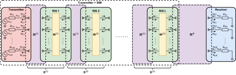
Figure 1: SIM-aided communication system diagram.

II SIM-Aided System Model Based on
Multiport Network Theory

Consider a SIM-aided communication system between an $M$-antenna transmitter and a $K$-antenna receiver, as represented in Fig. 1. The SIM is deployed at the transmitter and is composed of $L$ layers, each being an $N$-element RIS. We model this SIM-aided system through multiport network theory as follows [10, Chapter 4].

At the transmitter, the $m$th antenna is connected in series with a source voltage $v_{s,m}$ and a source impedance $Z_{T,m}$, for $m=1,\ldots,M$. Defining $\mathbf{a}_{T}\in\mathbb{C}^{M\times 1}$ and $\mathbf{b}_{T}\in\mathbb{C}^{M\times 1}$ as the reflected and incident waves at the transmitter, we have

$$\mathbf{a}_{T}=\mathbf{b}_{s,T}+\mathbf{\Gamma}_{T}\mathbf{b}_{T},$$ (1)

where $\mathbf{\Gamma}_{T}\in\mathbb{C}^{M\times M}$ is a diagonal matrix containing the reflection coefficients of the source impedances, i.e.,

$$\mathbf{\Gamma}_{T}=\left(\mathbf{Z}_{T}+Z_{0}\mathbf{I}\right)^{-1}\left(\mathbf{Z}_{T}-Z_{0}\mathbf{I}\right),$$ (2)

with $\mathbf{Z}_{T}=\textrm{diag}(Z_{T,1},\ldots,Z_{T,M})$ and $Z_{0}$ denoting the reference impedance typically set to $Z_{0}=50$ $\Omega$, and $\mathbf{b}_{s,T}\in\mathbb{C}^{M\times 1}$ is the source wave vector given by $\mathbf{b}_{s,T}=(\mathbf{I}-\mathbf{\Gamma}_{T})\mathbf{v}_{s,T}/2$, with $\mathbf{v}_{s,T}=[v_{s,1},\ldots,v_{s,M}]^{T}$ [8].

The SIM is a cascade of $L$ blocks, each consisting of the cascade of a wireless channel and an RIS. Specifically, the $\ell$th block consists of the cascade of the wireless channel between the $(\ell-1)$th and the $\ell$th SIM layer and the RIS implementing the $\ell$th SIM layer, for $\ell=2,\ldots,L$. We model the channel between the $(\ell-1)$th and the $\ell$th SIM layer as a $2N$-port network with scattering matrix $\mathbf{H}^{(\ell)}\in\mathbb{C}^{2N\times 2N}$ given by

$$\mathbf{H}^{(\ell)}=\begin{bmatrix}\mathbf{H}_{11}^{(\ell)}&\mathbf{H}_{12}^{(\ell)}\\ \mathbf{H}_{21}^{(\ell)}&\mathbf{H}_{22}^{(\ell)}\end{bmatrix},$$ (3)

where $\mathbf{H}_{11}^{(\ell)}\in\mathbb{C}^{N\times N}$ and $\mathbf{H}_{22}^{(\ell)}\in\mathbb{C}^{N\times N}$ refer to the antenna mutual coupling at the $(\ell-1)$th and the $\ell$th SIM layer, respectively, and $\mathbf{H}_{21}^{(\ell)}\in\mathbb{C}^{N\times N}$ refer to the transmission scattering matrix from the $(\ell-1)$th to the $\ell$th SIM layer, for $\ell=2,\ldots,L$. Beside, we model the RIS at the $\ell$th SIM layer through its scattering matrix $\boldsymbol{\Theta}^{(\ell)}\in\mathbb{C}^{2N\times 2N}$ given by

$$\boldsymbol{\Theta}^{(\ell)}=\begin{bmatrix}\boldsymbol{\Theta}_{11}^{(\ell)}&\boldsymbol{\Theta}_{12}^{(\ell)}\\ \boldsymbol{\Theta}_{21}^{(\ell)}&\boldsymbol{\Theta}_{22}^{(\ell)}\end{bmatrix},$$ (4)

for $\ell=2,\ldots,L$, which is symmetric in the case of a reciprocal RIS and whose structure depends on the RIS architecture. In the case the SIM layers are implemented through conventional D-RISs, we have $\boldsymbol{\Theta}_{11}^{(\ell)}=\mathbf{0}$ and $\boldsymbol{\Theta}_{22}^{(\ell)}=\mathbf{0}$ since the RISs work in transmissive mode [11], and

$$\boldsymbol{\Theta}_{12}^{(\ell)}=\boldsymbol{\Theta}_{21}^{(\ell)}=\text{diag}\left(e^{j\theta_{1}^{(\ell)}},\ldots,e^{j\theta_{N}^{(\ell)}}\right),$$ (5)

assuming the RISs to be lossless [1, 2]. However, these constraints valid for D-RISs can be relaxed into the more general constraint $\boldsymbol{\Theta}^{(\ell)H}\boldsymbol{\Theta}^{(\ell)}=\mathbf{I}$ by implementing the SIM layers through BD-RISs [11].

Note that the first block, i.e., $\ell=1$, consists of the cascade of the wireless channel between the transmitter and the first SIM layer and the RIS implementing the first SIM layer. Thus, the scattering matrix of the wireless channel of the first block $\mathbf{H}^{(1)}\in\mathbb{C}^{(M+N)\times(M+N)}$ is given as in (3), where $\mathbf{H}_{11}^{(1)}\in\mathbb{C}^{M\times M}$ refer to the antenna mutual coupling at the transmitter. Besides the scattering matrix of the first SIM layer $\boldsymbol{\Theta}^{(1)}$ is given as in (4).

The wireless channel between the $L$th SIM layer and the receiver is modeled as an $(N+K)$-port network with scattering matrix $\mathbf{H}^{R}\in\mathbb{C}^{(N+K)\times(N+K)}$ given by

$$\mathbf{H}^{R}=\begin{bmatrix}\mathbf{H}_{11}^{R}&\mathbf{H}_{12}^{R}\\ \mathbf{H}_{21}^{R}&\mathbf{H}_{22}^{R}\end{bmatrix},$$ (6)

where $\mathbf{H}_{11}^{R}\in\mathbb{C}^{N\times N}$ and $\mathbf{H}_{22}^{R}\in\mathbb{C}^{K\times K}$ refer to the antenna mutual coupling at the $L$th SIM layer and the receiver, respectively, and $\mathbf{H}_{21}^{R}\in\mathbb{C}^{K\times N}$ refer to the transmission scattering matrix from the $L$th SIM layer to the receiver.

At the receiver, the $k$th antenna is connected in series with a load impedance $Z_{R,k}$, for $k=1,\ldots,K$. Defining $\mathbf{a}_{R}\in\mathbb{C}^{K\times 1}$ and $\mathbf{b}_{R}\in\mathbb{C}^{K\times 1}$ the reflected and incident waves at the receiver, we have

$$\mathbf{a}_{R}=\mathbf{\Gamma}_{R}\mathbf{b}_{R},$$ (7)

where $\mathbf{\Gamma}_{R}\in\mathbb{C}^{K\times K}$ is a diagonal matrix containing the reflection coefficients of the load impedances, i.e.,

$$\mathbf{\Gamma}_{R}=\left(\mathbf{Z}_{R}+Z_{0}\mathbf{I}\right)^{-1}\left(\mathbf{Z}_{R}-Z_{0}\mathbf{I}\right),$$ (8)

with $\mathbf{Z}_{R}=\textrm{diag}(Z_{R,1},\ldots,Z_{R,K})$ [8].

III General SIM-Aided Channel Model

Our goal is to determine the expression of the channel matrix $\mathbf{H}\in\mathbb{C}^{K\times M}$ relating the voltage vector at the transmitter $\mathbf{v}_{T}\in\mathbb{C}^{M\times 1}$ and the voltage vector at the receiver $\mathbf{v}_{R}\in\mathbb{C}^{K\times 1}$ though $\mathbf{v}_{R}=\mathbf{H}\mathbf{v}_{T}$, where $\mathbf{v}_{T}$ and $\mathbf{v}_{R}$ are given by

$$\mathbf{v}_{T}=\mathbf{a}_{T}+\mathbf{b}_{T},\>\mathbf{v}_{R}=\mathbf{a}_{R}+\mathbf{b}_{R},$$ (9)

according to multiport network theory [10, Chapter 4]. To this end, we introduce a proposition enabling the analysis of the considered SIM-aided system.

Proposition 1.

Consider the cascade system represented in Fig. 2, consisting of an $N_{P}$-port network, with scattering matrix $\mathbf{P}\in\mathbb{C}^{N_{P}\times N_{P}}$ given by

$$\mathbf{P}=\begin{bmatrix}\mathbf{P}_{11}&\mathbf{P}_{12}\\ \mathbf{P}_{21}&\mathbf{P}_{22}\end{bmatrix},$$ (10)

where $\mathbf{P}_{11}\in\mathbb{C}^{N_{1}\times N_{1}}$ and $\mathbf{P}_{22}\in\mathbb{C}^{N_{2}\times N_{2}}$, with $N_{P}=N_{1}+N_{2}$, and an $N_{Q}$-port network, with scattering matrix $\mathbf{Q}\in\mathbb{C}^{N_{Q}\times N_{Q}}$ given by

$$\mathbf{Q}=\begin{bmatrix}\mathbf{Q}_{11}&\mathbf{Q}_{12}\\ \mathbf{Q}_{21}&\mathbf{Q}_{22}\end{bmatrix},$$ (11)

where $\mathbf{Q}_{11}\in\mathbb{C}^{N_{2}\times N_{2}}$ and $\mathbf{Q}_{22}\in\mathbb{C}^{N_{3}\times N_{3}}$, with $N_{Q}=N_{2}+N_{3}$. In this cascade, the last $N_{2}$ ports of the $N_{P}$-port network are individually connected to the first $N_{2}$ ports of the $N_{Q}$-port network. Thus, the whole cascade can be regarded as an $N_{R}$-port network, where $N_{R}=N_{1}+N_{3}$, with scattering matrix $\mathbf{R}\in\mathbb{C}^{N_{R}\times N_{R}}$ given by

$$\mathbf{R}=\begin{bmatrix}\mathbf{R}_{11}&\mathbf{R}_{12}\\ \mathbf{R}_{21}&\mathbf{R}_{22}\end{bmatrix},$$ (12)

with

$$\mathbf{R}_{11}=\mathbf{P}_{11}+\mathbf{P}_{12}\left(\mathbf{I}-\mathbf{Q}_{11}\mathbf{P}_{22}\right)^{-1}\mathbf{Q}_{11}\mathbf{P}_{21},$$ (13)

$$\mathbf{R}_{12}=\mathbf{P}_{12}\left(\mathbf{I}-\mathbf{Q}_{11}\mathbf{P}_{22}\right)^{-1}\mathbf{Q}_{12},$$ (14)

$$\mathbf{R}_{21}=\mathbf{Q}_{21}\left(\mathbf{I}-\mathbf{P}_{22}\mathbf{Q}_{11}\right)^{-1}\mathbf{P}_{21},$$ (15)

$$\mathbf{R}_{22}=\mathbf{Q}_{22}+\mathbf{Q}_{21}\left(\mathbf{I}-\mathbf{P}_{22}\mathbf{Q}_{11}\right)^{-1}\mathbf{P}_{22}\mathbf{Q}_{12}.$$ (16)

Proof.

Please refer to the Appendix. ∎

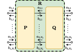
Figure 2: Cascade of two multiport networks.

To derive the expression of $\mathbf{H}$, we first recall that the $\ell$th block of the SIM is formed by the cascade of the channel $\mathbf{H}^{(\ell)}$ and the RIS $\boldsymbol{\Theta}^{(\ell)}$, given by (3) and (4), respectively. Thus, the scattering matrix of the $\ell$th block is given by

$$\mathbf{S}^{(\ell)}=\begin{bmatrix}\mathbf{S}_{11}^{(\ell)}&\mathbf{S}_{12}^{(\ell)}\\ \mathbf{S}_{21}^{(\ell)}&\mathbf{S}_{22}^{(\ell)}\end{bmatrix},$$ (17)

with

$$\mathbf{S}_{11}^{(\ell)}=\mathbf{H}_{11}^{(\ell)}+\mathbf{H}_{12}^{(\ell)}\left(\mathbf{I}-\boldsymbol{\Theta}_{11}^{(\ell)}\mathbf{H}_{22}^{(\ell)}\right)^{-1}\boldsymbol{\Theta}_{11}^{(\ell)}\mathbf{H}_{21}^{(\ell)},$$ (18)

$$\mathbf{S}_{12}^{(\ell)}=\mathbf{H}_{12}^{(\ell)}\left(\mathbf{I}-\boldsymbol{\Theta}_{11}^{(\ell)}\mathbf{H}_{22}^{(\ell)}\right)^{-1}\boldsymbol{\Theta}_{12}^{(\ell)},$$ (19)

$$\mathbf{S}_{21}^{(\ell)}=\boldsymbol{\Theta}_{21}^{(\ell)}\left(\mathbf{I}-\mathbf{H}_{22}^{(\ell)}\boldsymbol{\Theta}_{11}^{(\ell)}\right)^{-1}\mathbf{H}_{21}^{(\ell)},$$ (20)

$$\mathbf{S}_{22}^{(\ell)}=\boldsymbol{\Theta}_{22}^{(\ell)}+\boldsymbol{\Theta}_{21}^{(\ell)}\left(\mathbf{I}-\mathbf{H}_{22}^{(\ell)}\boldsymbol{\Theta}_{11}^{(\ell)}\right)^{-1}\mathbf{H}_{22}^{(\ell)}\boldsymbol{\Theta}_{12}^{(\ell)},$$ (21)

for $\ell=1,\ldots,L$, following Proposition 16. Given $\mathbf{S}^{(\ell)}$, the equivalent scattering matrix including the first $\ell$ blocks of the SIM can be determined recursively by

$$\bar{\mathbf{S}}^{(\ell)}=\begin{bmatrix}\bar{\mathbf{S}}_{11}^{(\ell)}&\bar{\mathbf{S}}_{12}^{(\ell)}\\ \bar{\mathbf{S}}_{21}^{(\ell)}&\bar{\mathbf{S}}_{22}^{(\ell)}\end{bmatrix},$$ (22)

with

$$\bar{\mathbf{S}}_{11}^{(\ell)}=\bar{\mathbf{S}}_{11}^{(\ell-1)}+\bar{\mathbf{S}}_{12}^{(\ell-1)}\left(\mathbf{I}-\mathbf{S}_{11}^{(\ell)}\bar{\mathbf{S}}_{22}^{(\ell-1)}\right)^{-1}\mathbf{S}_{11}^{(\ell)}\bar{\mathbf{S}}_{21}^{(\ell-1)},$$ (23)

$$\bar{\mathbf{S}}_{12}^{(\ell)}=\bar{\mathbf{S}}_{12}^{(\ell-1)}\left(\mathbf{I}-\mathbf{S}_{11}^{(\ell)}\bar{\mathbf{S}}_{22}^{(\ell-1)}\right)^{-1}\mathbf{S}_{12}^{(\ell)},$$ (24)

$$\bar{\mathbf{S}}_{21}^{(\ell)}=\mathbf{S}_{21}^{(\ell)}\left(\mathbf{I}-\bar{\mathbf{S}}_{22}^{(\ell-1)}\mathbf{S}_{11}^{(\ell)}\right)^{-1}\bar{\mathbf{S}}_{21}^{(\ell-1)},$$ (25)

$$\bar{\mathbf{S}}_{22}^{(\ell)}=\mathbf{S}_{22}^{(\ell)}+\mathbf{S}_{21}^{(\ell)}\left(\mathbf{I}-\bar{\mathbf{S}}_{22}^{(\ell-1)}\mathbf{S}_{11}^{(\ell)}\right)^{-1}\bar{\mathbf{S}}_{22}^{(\ell-1)}\mathbf{S}_{12}^{(\ell)},$$ (26)

as a function of $\bar{\mathbf{S}}^{(\ell-1)}$ and $\mathbf{S}^{(\ell)}$, where $\bar{\mathbf{S}}^{(1)}=\mathbf{S}^{(1)}$, according to Proposition 16. In particular, $\bar{\mathbf{S}}^{(L)}$ represents the equivalent scattering matrix including all the $L$ blocks of the SIM. From $\bar{\mathbf{S}}^{(L)}$ and the channel $\mathbf{H}^{R}$, the scattering matrix of the entire channel between the transmitter and the receiver is given by the cascade of $\bar{\mathbf{S}}^{(L)}$ and $\mathbf{H}^{R}$, and writes as

$$\mathbf{S}=\begin{bmatrix}\mathbf{S}_{11}&\mathbf{S}_{12}\\ \mathbf{S}_{21}&\mathbf{S}_{22}\end{bmatrix},$$ (27)

with

$$\mathbf{S}_{11}=\bar{\mathbf{S}}_{11}^{(L)}+\bar{\mathbf{S}}_{12}^{(L)}\left(\mathbf{I}-\mathbf{H}_{11}^{R}\bar{\mathbf{S}}_{22}^{(L)}\right)^{-1}\mathbf{H}_{11}^{R}\bar{\mathbf{S}}_{21}^{(L)},$$ (28)

$$\mathbf{S}_{12}=\bar{\mathbf{S}}_{12}^{(L)}\left(\mathbf{I}-\mathbf{H}_{11}^{R}\bar{\mathbf{S}}_{22}^{(L)}\right)^{-1}\mathbf{H}_{12}^{R},$$ (29)

$$\mathbf{S}_{21}=\mathbf{H}_{21}^{R}\left(\mathbf{I}-\bar{\mathbf{S}}_{22}^{(L)}\mathbf{H}_{11}^{R}\right)^{-1}\bar{\mathbf{S}}_{21}^{(L)},$$ (30)

$$\mathbf{S}_{22}=\mathbf{H}_{22}^{R}+\mathbf{H}_{21}^{R}\left(\mathbf{I}-\bar{\mathbf{S}}_{22}^{(L)}\mathbf{H}_{11}^{R}\right)^{-1}\bar{\mathbf{S}}_{22}^{(L)}\mathbf{H}_{12}^{R},$$ (31)

according to Proposition 16.

To express $\mathbf{H}$ as a function of $\mathbf{S}$, we consider $\mathbf{Z}_{T}=Z_{0}\mathbf{I}$ and $\mathbf{Z}_{R}=Z_{0}\mathbf{I}$ for simplicity, so that $\mathbf{\Gamma}_{T}=\mathbf{0}$ and $\mathbf{\Gamma}_{R}=\mathbf{0}$ according to (2) and (8), respectively. Consequently, $\mathbf{H}$ can be derived by solving the system

$$\begin{bmatrix}\mathbf{b}_{T}\\ \mathbf{b}_{R}\end{bmatrix}=\begin{bmatrix}\mathbf{S}_{11}&\mathbf{S}_{12}\\ \mathbf{S}_{21}&\mathbf{S}_{22}\end{bmatrix}\begin{bmatrix}\mathbf{a}_{T}\\ \mathbf{a}_{R}\end{bmatrix},$$ (32)

$$\mathbf{a}_{T}=\mathbf{b}_{s,T},\>\mathbf{a}_{R}=\mathbf{0},$$ (33)

$$\eqref{eq:vtvr},$$ (34)

where (32) follows the definition of scattering matrix [10, Chapter 4] and (33) is given by (1) and (7). Since it is possible to show that system (32)-(34) yields $\mathbf{v}_{R}=\mathbf{S}_{21}\left(\mathbf{I}+\mathbf{S}_{11}\right)^{-1}\mathbf{v}_{T}$, we have

$$\mathbf{H}=\mathbf{S}_{21}\left(\mathbf{I}+\mathbf{S}_{11}\right)^{-1},$$ (35)

giving the general expression of a SIM-aided channel. Remarkably, it is hard to understand the role of the reconfigurable scattering matrices $\boldsymbol{\Theta}^{(\ell)}$ in (35). For this reason, we simplify this channel model and show under which assumptions it boils down to the easier model widely used in recent works on SIM.

IV Simplified SIM-Aided Channel Model

To simplify the channel model in (35), we assume that the unilateral approximation is valid in all the channels $\mathbf{H}^{(\ell)}$, i.e., $\mathbf{H}_{12}^{(\ell)}=\mathbf{0}$, for $\ell=1,\ldots,L$ [12]. In other words, we assume that the electrical properties at the $(\ell-1)$th SIM layer are independent of the electrical properties at the $\ell$th SIM layer (where the $0$th SIM layer means the transmitter). Given the short transmission distances in a SIM architecture, extensive electromagnetic simulations are needed to verify the validity of this assumption, which is beyond the scope of this study. In addition, we assume no mutual coupling between the transmit antennas and between the RIS elements, i.e., $\mathbf{H}_{11}^{(\ell)}=\mathbf{0}$ and $\mathbf{H}_{22}^{(\ell)}=\mathbf{0}$, for $\ell=1,\ldots,L$, and $\mathbf{H}_{11}^{R}=\mathbf{0}$. With these assumptions, the scattering matrix of the $\ell$th block of the SIM given by (17) simplifies as

$$\mathbf{S}^{(\ell)}=\begin{bmatrix}\mathbf{0}&\mathbf{0}\\ \boldsymbol{\Theta}_{21}^{(\ell)}\mathbf{H}_{21}^{(\ell)}&\boldsymbol{\Theta}_{22}^{(\ell)}\end{bmatrix},$$ (36)

for $\ell=1,\ldots,L$. Thus, the equivalent scattering matrix of the first $\ell$ blocks of the SIM is given recursively as

$$\bar{\mathbf{S}}^{(\ell)}=\begin{bmatrix}\bar{\mathbf{S}}_{11}^{(\ell-1)}&\mathbf{0}\\ \mathbf{S}_{21}^{(\ell)}\bar{\mathbf{S}}_{21}^{(\ell-1)}&\mathbf{S}_{22}^{(\ell)}\end{bmatrix},$$ (37)

where $\bar{\mathbf{S}}^{(1)}=\mathbf{S}^{(1)}$. Consequently, the equivalent scattering matrix including all the $L$ blocks of the SIM can now be written in closed-form as

$$\bar{\mathbf{S}}^{(L)}=\begin{bmatrix}\mathbf{0}&\mathbf{0}\\ \boldsymbol{\Theta}_{21}^{(L)}\mathbf{H}_{21}^{(L)}\cdots\boldsymbol{\Theta}_{21}^{(2)}\mathbf{H}_{21}^{(2)}\boldsymbol{\Theta}_{21}^{(1)}\mathbf{H}_{21}^{(1)}&\boldsymbol{\Theta}_{22}^{(L)}\end{bmatrix}.$$ (38)

Given $\bar{\mathbf{S}}^{(L)}$ and $\mathbf{H}^{R}$, the scattering matrix of the entire channel between the transmitter and the receiver writes as

$$\mathbf{S}=\begin{bmatrix}\mathbf{0}&\mathbf{0}\\ \mathbf{H}_{21}^{R}\boldsymbol{\Theta}_{21}^{(L)}\mathbf{H}_{21}^{(L)}\cdots\boldsymbol{\Theta}_{21}^{(1)}\mathbf{H}_{21}^{(1)}&\mathbf{H}_{22}^{R}+\mathbf{H}_{21}^{R}\boldsymbol{\Theta}_{22}^{(L)}\mathbf{H}_{12}^{R}\end{bmatrix},$$ (39)

by Proposition 16. By substituting (39) into (35), and using the auxiliary notation $\bar{\mathbf{H}}^{R}=\mathbf{H}_{21}^{R}$, $\bar{\boldsymbol{\Theta}}^{(\ell)}=\boldsymbol{\Theta}_{21}^{(\ell)}$, and $\bar{\mathbf{H}}^{(\ell)}=\mathbf{H}_{21}^{(\ell)}$, for $\ell=1,\ldots,L$, we finally obtain

$$\mathbf{H}=\bar{\mathbf{H}}^{R}\bar{\boldsymbol{\Theta}}^{(L)}\bar{\mathbf{H}}^{(L)}\cdots\bar{\boldsymbol{\Theta}}^{(2)}\bar{\mathbf{H}}^{(2)}\bar{\boldsymbol{\Theta}}^{(1)}\bar{\mathbf{H}}^{(1)},$$ (40)

which is the simplified channel model, in agreement with the model widely utilized in recent works [1, 2, 6].

V Implementing SIM with D-RIS and BD-RIS

Consider a single-input single-output (SISO) system, i.e., $M=1$ and $K=1$, where we maximize the channel gain

$$\left|h\right|^{2}=\left|\bar{\mathbf{h}}^{R}\bar{\boldsymbol{\Theta}}^{(L)}\bar{\mathbf{H}}^{(L)}\cdots\bar{\boldsymbol{\Theta}}^{(2)}\bar{\mathbf{H}}^{(2)}\bar{\boldsymbol{\Theta}}^{(1)}\bar{\mathbf{h}}^{(1)}\right|^{2},$$ (41)

by optimizing the SIM, i.e., $\bar{\boldsymbol{\Theta}}^{(\ell)}$, for $\ell=1,\ldots,L$.

In the case of a SIM implemented with D-RIS, $\bar{\boldsymbol{\Theta}}^{(\ell)}$ are subject to (5) and a generous upper bound on the achievable channel gain is given by

$$\left|h^{\text{D-RIS}}\right|^{2}\leq\left\|\bar{\mathbf{h}}^{R}\right\|^{2}\left\|\bar{\mathbf{H}}^{(L)}\right\|^{2}\cdots\left\|\bar{\mathbf{H}}^{(2)}\right\|^{2}\left\|\bar{\mathbf{h}}^{(1)}\right\|^{2},$$ (42)

following the submultiplicativity property of the spectral norm and noticing that $\|\bar{\boldsymbol{\Theta}}^{(\ell)}\|=1$, for $\ell=1,\ldots,L$. To optimize the SIM, we propose an iterative algorithm that optimizes a matrix $\bar{\boldsymbol{\Theta}}^{(\ell)}$ at each iteration through a closed-form globally optimal solution. Specifically, at each iteration, $\bar{\boldsymbol{\Theta}}^{(\ell)}$ is updated by introducing $\mathbf{u}^{(\ell)}=\bar{\mathbf{h}}^{R}\bar{\boldsymbol{\Theta}}^{(L)}\bar{\mathbf{H}}^{(L)}\cdots\bar{\boldsymbol{\Theta}}^{(\ell+1)}\bar{\mathbf{H}}^{(\ell+1)}$ and $\mathbf{v}^{(\ell)}=\bar{\mathbf{H}}^{(\ell)}\bar{\boldsymbol{\Theta}}^{(\ell-1)}\bar{\mathbf{H}}^{(\ell-1)}\cdots\bar{\boldsymbol{\Theta}}^{(1)}\bar{\mathbf{h}}^{(1)}$, and setting $\theta_{n}^{(\ell)}=-\mathrm{arg}([\mathbf{u}^{(\ell)}]_{n}[\mathbf{v}^{(\ell)}]_{n})$, for $n=1,\ldots,N$. The algorithm iterates until convergence of the objective (41). In terms of circuit complexity, when the SIM layers are implemented through D-RISs working in transmissive mode, the number of tunable impedances in the circuit topology is $3N$ per layer [11], yielding $3NL$ total tunable impedances in the SIM architecture.

In the case of a SIM implemented with BD-RIS, we first consider $L=1$ and we show that this is the optimal number of layers. When $L=1$, (41) boils down to $|h|^{2}=|\bar{\mathbf{h}}^{R}\bar{\boldsymbol{\Theta}}^{(1)}\bar{\mathbf{h}}^{(1)}|^{2}$, which can be rewritten as $|h|^{2}=|[\mathbf{0},\bar{\mathbf{h}}^{R}]\boldsymbol{\Theta}^{(1)}[\bar{\mathbf{h}}^{(1)T},\mathbf{0}]^{T}|^{2}$, where $\mathbf{0}$ denotes here a $1\times N$ zero vector and $\boldsymbol{\Theta}^{(1)}$ is subject to $\boldsymbol{\Theta}^{(1)}=\boldsymbol{\Theta}^{(1)T}$ and $\boldsymbol{\Theta}^{(1)H}\boldsymbol{\Theta}^{(1)}=\mathbf{I}$. Interestingly, it has been shown in [13] that $\boldsymbol{\Theta}^{(1)}$ can be optimized to obtain

$$\left|h^{\text{BD-RIS}}\right|^{2}=\left\|\bar{\mathbf{h}}^{R}\right\|^{2}\left\|\bar{\mathbf{h}}^{(1)}\right\|^{2}.$$ (43)

Besides, the performance upper bound in (43) can also be achieved with low-complexity BD-RIS architectures denoted as tree-connected RISs through a closed-form solution [5]. Since it holds that $\|\bar{\mathbf{H}}^{(\ell)}\|<1$ for the wireless channels $\bar{\mathbf{H}}^{(\ell)}$, the upper bound in (43) is always greater than (42). Thus, $L=1$ is the optimal number of layers in a SIM implemented with tree-connected RISs. Furthermore, we have $\left|h^{\text{D-RIS}}\right|^{2}\leq\left|h^{\text{BD-RIS}}\right|^{2}$ as a consequence of (42) and (43). Considering a 1-layer SIM implemented through a tree-connected RIS, the number of needed tunable impedances is $4N-1$ [5].

VI Numerical Results

Consider a 3-dimensional coordinate system $(x,y,z)$ in which we locate a SISO system between a SIM-aided transmitter and a receiver. The transmit antenna is located at $(0,0,0)$ and the SIM layers are $N_{x}\times N_{y}$ uniform planar arrays (UPAs) parallel to the $x$-$y$ plane and centered in $(0,0)$. The first SIM layer is spaced $\lambda$ from the transmit antenna and the SIM layers are spaced $\lambda$ from each other, where $\lambda$ denotes the wavelength. The RIS elements in each SIM layer have inter-element distance $\lambda/2$ and we set $N_{x}=4$ and carrier frequency 28 GHz. The channels $\bar{\mathbf{H}}^{(\ell)}$, for $\ell=1,\ldots,L$, are modeled using Rayleigh-Sommerfield’s diffraction theory as

$$\left[\bar{\mathbf{H}}^{(\ell)}\right]_{i,j}=\frac{A\cos\left(\alpha_{i,j}^{(\ell)}\right)}{d_{i,j}^{(\ell)}}\left(\frac{1}{2\pi d_{i,j}^{(\ell)}}-j\frac{1}{\lambda}\right)e^{j2\pi d_{i,j}^{(\ell)}/\lambda},$$ (44)

where $A=(\lambda/2)^{2}$ is the area of each RIS element, $\alpha_{i,j}^{(\ell)}$ is the angle between the normal of the $(\ell-1)$th SIM layer and the propagation direction and $d_{i,j}^{(\ell)}$ is the transmission distance [1]. Besides, the channel $\bar{\mathbf{h}}^{R}$ is modeled as independent and identically distributed (i.i.d.) Rayleigh distributed.

In Fig. 3, we report the performance in terms of normalized channel gain, defined as $G=|h|^{2}/(\|\bar{\mathbf{h}}^{R}\|^{2}\|\bar{\mathbf{h}}^{(1)}\|^{2})$, achieved by SIM implemented with D-RIS and BD-RIS. For SIM implemented with BD-RIS, we consider a 1-layer SIM implemented through a tree-connected RIS, optimized as proposed in [5]. We make the following observations. First, 1-layer SIMs implemented with BD-RIS always achieve $G=1$, i.e., the performance upper bound, as expected from (43). Second, SIMs implemented with D-RIS always underperform 1-layer SIMs implemented with BD-RIS, in agreement with our theoretical derivations. Third, for a low number of RIS elements $N$, SIMs with a low number of layers $L$ are beneficial. This is because a low $N$ reduces the norms $\|\bar{\mathbf{H}}^{(\ell)}\|$, for $\ell=1,\ldots,L$, which are always $\|\bar{\mathbf{H}}^{(\ell)}\|<1$. Consequently, when $\|\bar{\mathbf{H}}^{(\ell)}\|<<1$, a high $L$ is suboptimal as it limits the product in the performance upper bound (42). Fourth, for a high value of $N$, SIMs with more layers are beneficial given their enhanced flexibility.

In Fig. 3, we also report the circuit complexity of the considered SIM architectures, in terms of the number of tunable impedance components in the circuit topology. Interestingly, we observe that 1-layer SIMs implemented with BD-RIS are also favorable in terms of complexity, as they are slightly more complex than 1-layer SIMs implemented with D-RIS.

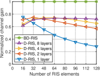
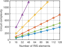
Figure 3: Normalized channel gain $G=|h|^{2}/(\|\bar{\mathbf{h}}^{R}\|^{2}\|\bar{\mathbf{h}}^{(1)}\|^{2})$ and circuit complexity of SIM implemented with D-RIS and BD-RIS.

VII Conclusion

We analyze SIM-aided communication systems by using multiport network theory and derive a physically consistent SIM-aided channel model. To understand the role of the SIM on the derived model, we make specific assumptions to obtain a simplified channel model that is consistent with the model employed in previous works on SIM. With this simplified model, we compare SIM implemented with D-RIS and BD-RIS, showing that 1-layer SIM implemented with BD-RIS outperforms any $L$-layer SIM implemented with D-RIS.

Appendix

Denote as $\mathbf{a}_{1}=[a_{1,1},\ldots,a_{1,N_{1}}]^{T}$ and $\mathbf{b}_{1}=[b_{1,1},\ldots,b_{1,N_{1}}]^{T}$ the incident and reflected waves on the first $N_{1}$ ports of the $N_{P}$-port network, respectively; as $\mathbf{a}_{2}=[a_{2,1},\ldots,a_{2,N_{2}}]^{T}$ and $\mathbf{b}_{2}=[b_{2,1},\ldots,b_{2,N_{2}}]^{T}$ the incident and reflected waves on the last $N_{2}$ ports of the $N_{P}$-port network, respectively; and as $\mathbf{a}_{3}=[a_{3,1},\ldots,a_{3,N_{3}}]^{T}$ and $\mathbf{b}_{3}=[b_{3,1},\ldots,b_{3,N_{3}}]^{T}$ the reflected and incident waves on the last $N_{3}$ ports of the $N_{Q}$-port network, respectively. Given the interconnections between the two multiport networks, $\mathbf{a}_{2}$ and $\mathbf{b}_{2}$ are also the reflected and incident waves on the first $N_{2}$ ports of the $N_{Q}$-port network, respectively. Thus, we have

$$\begin{bmatrix}\mathbf{b}_{1}\\ \mathbf{b}_{2}\end{bmatrix}=\begin{bmatrix}\mathbf{P}_{11}&\mathbf{P}_{12}\\ \mathbf{P}_{21}&\mathbf{P}_{22}\end{bmatrix}\begin{bmatrix}\mathbf{a}_{1}\\ \mathbf{a}_{2}\end{bmatrix},\>\begin{bmatrix}\mathbf{a}_{2}\\ \mathbf{a}_{3}\end{bmatrix}=\begin{bmatrix}\mathbf{Q}_{11}&\mathbf{Q}_{12}\\ \mathbf{Q}_{21}&\mathbf{Q}_{22}\end{bmatrix}\begin{bmatrix}\mathbf{b}_{2}\\ \mathbf{b}_{3}\end{bmatrix},$$ (45)

and our goal is to characterize $\mathbf{R}$ such that

$$\begin{bmatrix}\mathbf{b}_{1}\\ \mathbf{a}_{3}\end{bmatrix}=\begin{bmatrix}\mathbf{R}_{11}&\mathbf{R}_{12}\\ \mathbf{R}_{21}&\mathbf{R}_{22}\end{bmatrix}\begin{bmatrix}\mathbf{a}_{1}\\ \mathbf{b}_{3}\end{bmatrix},$$ (46)

according to [10, Chapter 4]. To this end, we first use (45) to express $\mathbf{a}_{2}$ and $\mathbf{b}_{2}$ as functions of $\mathbf{a}_{1}$ and $\mathbf{b}_{3}$ as

$$\mathbf{a}_{2}=\left(\mathbf{I}-\mathbf{Q}_{11}\mathbf{P}_{22}\right)^{-1}\mathbf{Q}_{11}\mathbf{P}_{21}\mathbf{a}_{1}+\left(\mathbf{I}-\mathbf{Q}_{11}\mathbf{P}_{22}\right)^{-1}\mathbf{Q}_{12}\mathbf{b}_{3},$$ (47)

$$\mathbf{b}_{2}=\left(\mathbf{I}-\mathbf{P}_{22}\mathbf{Q}_{11}\right)^{-1}\mathbf{P}_{21}\mathbf{a}_{1}+\left(\mathbf{I}-\mathbf{P}_{22}\mathbf{Q}_{11}\right)^{-1}\mathbf{P}_{22}\mathbf{Q}_{12}\mathbf{b}_{3}.$$ (48)

Then, by substituting (47) into $\mathbf{b}_{1}=\mathbf{P}_{11}\mathbf{a}_{1}+\mathbf{P}_{12}\mathbf{a}_{2}$, which is derived from (45), we obtain

$$\mathbf{b}_{1}=\mathbf{P}_{11}\mathbf{a}_{1}+\mathbf{P}_{12}\left(\mathbf{I}-\mathbf{Q}_{11}\mathbf{P}_{22}\right)^{-1}\mathbf{Q}_{11}\mathbf{P}_{21}\mathbf{a}_{1}\\ +\mathbf{P}_{12}\left(\mathbf{I}-\mathbf{Q}_{11}\mathbf{P}_{22}\right)^{-1}\mathbf{Q}_{12}\mathbf{b}_{3},$$ (49)

and by substituting (48) into $\mathbf{a}_{3}=\mathbf{Q}_{21}\mathbf{b}_{2}+\mathbf{Q}_{22}\mathbf{b}_{3}$, we obtain

$$\mathbf{a}_{3}=\mathbf{Q}_{21}\left(\mathbf{I}-\mathbf{P}_{22}\mathbf{Q}_{11}\right)^{-1}\mathbf{P}_{21}\mathbf{a}_{1}\\ +\mathbf{Q}_{21}\left(\mathbf{I}-\mathbf{P}_{22}\mathbf{Q}_{11}\right)^{-1}\mathbf{P}_{22}\mathbf{Q}_{12}\mathbf{b}_{3}+\mathbf{Q}_{22}\mathbf{b}_{3},$$ (50)

proving the proposition.

References

• [1] J. An, M. Di Renzo, M. Debbah, and C. Yuen, “Stacked intelligent metasurfaces for multiuser beamforming in the wave domain,” in ICC 2023 - IEEE International Conference on Communications, 2023, pp. 2834–2839.
• [2] J. An, C. Xu, D. W. K. Ng, G. C. Alexandropoulos, C. Huang, C. Yuen, and L. Hanzo, “Stacked intelligent metasurfaces for efficient holographic MIMO communications in 6G,” IEEE J. Sel. Areas Commun., vol. 41, no. 8, pp. 2380–2396, 2023.
• [3] H. Li, S. Shen, M. Nerini, and B. Clerckx, “Reconfigurable intelligent surfaces 2.0: Beyond diagonal phase shift matrices,” IEEE Commun. Mag., 2023.
• [4] S. Shen, B. Clerckx, and R. Murch, “Modeling and architecture design of reconfigurable intelligent surfaces using scattering parameter network analysis,” IEEE Trans. Wireless Commun., vol. 21, no. 2, pp. 1229–1243, 2022.
• [5] M. Nerini, S. Shen, H. Li, and B. Clerckx, “Beyond diagonal reconfigurable intelligent surfaces utilizing graph theory: Modeling, architecture design, and optimization,” arXiv preprint arXiv:2305.05013, 2023.
• [6] N. U. Hassan, J. An, M. Di Renzo, M. Debbah, and C. Yuen, “Efficient beamforming and radiation pattern control using stacked intelligent metasurfaces,” IEEE Open J. Commun. Soc., vol. 5, pp. 599–611, 2024.
• [7] G. Gradoni and M. Di Renzo, “End-to-end mutual coupling aware communication model for reconfigurable intelligent surfaces: An electromagnetic-compliant approach based on mutual impedances,” IEEE Wireless Commun. Lett., vol. 10, no. 5, pp. 938–942, 2021.
• [8] M. Nerini, S. Shen, H. Li, M. Di Renzo, and B. Clerckx, “A universal framework for multiport network analysis of reconfigurable intelligent surfaces,” arXiv preprint arXiv:2311.10561, 2023.
• [9] J. A. Nossek, D. Semmler, M. Joham, and W. Utschick, “Physically consistent modelling of wireless links with reconfigurable intelligent surfaces using multiport network analysis,” arXiv preprint arXiv:2308.12223, 2023.
• [10] D. M. Pozar, Microwave engineering.   John wiley & sons, 2011.
• [11] H. Li, S. Shen, and B. Clerckx, “Beyond diagonal reconfigurable intelligent surfaces: From transmitting and reflecting modes to single-, group-, and fully-connected architectures,” IEEE Trans. Wireless Commun., vol. 22, no. 4, pp. 2311–2324, 2023.
• [12] M. T. Ivrlač and J. A. Nossek, “Toward a circuit theory of communication,” IEEE Trans. Circuits Syst. I: Regul. Pap., vol. 57, no. 7, pp. 1663–1683, 2010.
• [13] M. Nerini, S. Shen, and B. Clerckx, “Closed-form global optimization of beyond diagonal reconfigurable intelligent surfaces,” IEEE Trans. Wireless Commun., vol. 23, no. 2, pp. 1037–1051, 2024.