Deep Pa$\beta$ Imaging of the Candidate Accreting Protoplanet AB Aur b

Abstract

Giant planets grow by accreting gas through circumplanetary disks, but little is known about the timescale and mechanisms involved in the planet assembly process because few accreting protoplanets have been discovered. Recent visible and infrared (IR) imaging revealed a potential accreting protoplanet within the transition disk around the young intermediate-mass Herbig Ae star, AB Aurigae (AB Aur). Additional imaging in H$\alpha$ probed for accretion and found agreement between the line-to-continuum flux ratio of the star and companion, raising the possibility that the emission source could be a compact disk feature seen in scattered starlight. We present new deep Keck/NIRC2 high-contrast imaging of AB Aur to characterize emission in Pa$\beta$, another accretion tracer less subject to extinction. Our narrow band observations reach a 5$\sigma$ contrast of 9.6 mag at 0$\farcs$6, but we do not detect significant emission at the expected location of the companion, nor from other any other source in the system. Our upper limit on Pa$\beta$ emission suggests that if AB Aur b is a protoplanet, it is not heavily accreting or accretion is stochastic and was weak during the observations.

1 Introduction

Direct observations of planetary assembly with high-contrast imaging offers a promising pathway to establish the timescale, location, and mechanisms of giant planet formation. Planets accrete mass from a circumplanetary disk, which may be continually fed by a circumstellar disk during an embedded phase. Recent modeling efforts have informed observations of planetary-mass accretion signatures (e.g., Thanathibodee et al. 2019; Szulágyi & Ercolano 2020; Aoyama et al. 2020; Marleau & Aoyama 2022; Choksi & Chiang 2022), predicting increased favorability of detection at wavelengths with strong accretion luminosity such as line emission from infalling hydrogen gas and excess emission in the UV continuum from accretion hot spots. Ultraviolet (UV) to near-infrared (NIR) imaging of a handful of wide accreting substellar companions show signatures that are consistent with theoretical predictions (e.g., CT Cha B, Schmidt et al. 2008; DH Tau B, Zhou et al. 2014; van Holstein et al. 2021; GQ Lup B, Zhou et al. 2014; Stolker et al. 2021; Demars et al. 2023; GSC 06214-00210 B, Seifahrt et al. 2007; Bowler et al. 2011; Zhou et al. 2014; van Holstein et al. 2021; Demars et al. 2023; SR 12 C, Santamaría-Miranda et al. 2018)—most notably strong H$\alpha$ and Pa$\beta$ emission, and relatively bright UV emission.

However, protoplanets still embedded in the circumstellar disk pose a challenge; distinguishing disk substructures such as concentrated unresolved clumps from bona fide accreting protoplanets is complex, and many claimed protoplanet candidates identified at thermal wavelengths and in H$\alpha$ emission have been debated (e.g., LkCa 15 bcd Thalmann et al. 2016; Mendigutía et al. 2018; Currie et al. 2019; HD 100546 bc Rameau et al. 2017; Follette et al. 2017; Sissa et al. 2018; HD 169142 bc Biller et al. 2014; Pohl et al. 2017; Ligi et al. 2018). PDS 70 b and c (Keppler et al., 2018; Wagner et al., 2018; Haffert et al., 2019) are the only uncontested accreting protoplanets. Recently, visible and IR imaging revealed a source of concentrated emission in the transition disk surrounding the young ($\approx$4–6 Myr; Guzmán-Díaz et al. 2021; Zhou et al. 2022) accreting A0 star AB Aurigae (Currie et al., 2022), which was interpreted as an embedded protoplanet at a projected separation of 0.6^′′ ($\approx 100$ au). This is near the location where a giant planet was predicted by Tang et al. (2017) via modeling the disk’s inner substructure. The source is spatially resolved in multiple datasets and may be tracing circumplanetary disk structure, an envelope, circumstellar disk substructure, or a combination of these.

Protoplanets that are embedded in transition disks are predicted to experience persistent accretion (e.g., Tanigawa et al. 2012; Szulágyi et al. 2014) and will therefore exhibit strong H$\alpha$ emission from gas that is excited or ionized by intense radiation from the accretion post-shock region (Aoyama et al., 2018). If the surrounding envelope is not optically thick, then some or all of this emission will escape. However, the central star in transition disk systems can itself accrete from an inner disk and will also exhibit hydrogen emission. In these cases, the spectrum of a bright unresolved dust feature in the disk seen in scattered light could resemble an accreting planet.

In the case of AB Aur, the host is accreting and shows strong and variable line emission (e.g., Harrington & Kuhn 2007; Costigan et al. 2014). For this reason, confirming the protoplanetary nature of AB Aur b requires careful disambiguation of its own emission from that of surrounding disk features seen in scattered light. Any difference in line strength relative to the continuum between AB Aur A and b would support the hypothesis that AB Aur b is a protoplanet and would point to emission being locally generated. On the contrary, a consistent line strength would suggest that AB Aur b is actually a compact disk feature seen in scattered starlight.

Zhou et al. (2022) used the Hubble Space Telescope (HST) to search for H$\alpha$ emission from AB Aur b using narrow band photometry and found that moderate H$\alpha$ excess is indeed present. In addition, the line-to-continuum ratio of the candidate planet and star are consistent, which calls into question whether the emission originates from planetary accretion or scattered emission. However, the observations were not obtained simultaneously, so the similarity could also be coincidental. New UV and optical HST imaging by Zhou et al. (2023) indicates that at short wavelengths, the emission from AB Aur b is dominated by scattered light from the host star.

If AB Aur b is an accreting planet, then higher-order emission lines such as Pa$\beta$ should also be present. Pa$\beta$ is advantageous in searching for distinct accretion signatures from AB Aur b because it is less affected by extinction from the disk in comparison to H$\alpha$. In addition, a possible complimentary outcome from a multi-wavelength analysis is a constraint on the line-of-sight dust extinction to the source. This could further inform strategies for future imaging of AB Aur b, for instance with the James Webb Space Telescope.

Here, we report the first constraints on Pa$\beta$ emission from AB Aur b from Angular Differential Imaging (ADI) observations obtained with Keck II/NIRC2. We also characterize the stellar NIR emission line properties of AB Aur with moderate-resolution 0.74–2.50 $\mu$m spectroscopy acquired with the NASA Infrared Telescope Facility (IRTF)/SpeX. We outline our observations and data reduction in Section 2. In Section 3, we present the results. See Section 4 for our discussion of the resulting contrast curve and constraint on Pa$\beta$ line strength. A summary of this work can be found in Section 5.

2 Observations

2.1 Keck II/NIRC2

Adaptive optics images were obtained on UT 2022 September 17 with the NIRC2 camera on the Keck II 10-meter Telescope (Wizinowich et al., 2000). The NIRC2 plate scale is 9.971 $\pm$ 0.004 mas px^-1 and the Position Angle (PA) of each column relative to North is 0.262 $\pm$ 0.020$\arcdeg$ (Service et al., 2016). Images were acquired in vertical angle mode. We used the central star AB Aur A ($G$ = 7.11 mag; Gaia Collaboration 2020) as a natural guide star. The seeing was stable at $\approx 0.5^{\prime\prime}$ throughout the observations. All images were read as a centered 512 $\times$ 512 subarray.

We acquired a sequence of 50 images in the Pa$\beta$ narrow band filter ($\lambda_{0}=1.2903$ $\mu$m, $\Delta\lambda=0.0193$ $\mu$m) using Angular Differential Imaging (ADI; Liu 2004; Marois et al. 2006). The ADI method requires that the telescope pupil remain fixed on the camera while the field of view (FOV) rotates around the star over time. Each image in the ADI sequence was taken with a 1 sec integration time and 20 coadds for a total time of 20 s per frame. The total angular rotation of the FOV was 57.9$\arcdeg$, and the total on-source exposure time in Pa$\beta$ was 16.7 min.

Because AB Aur saturates in the ADI frames, we also captured 25 frames in the Pa$\beta$ filter with exposure times of 0.2 sec, and 100 coadds. AB Aur A was not saturated in these frames, which enabled us to calibrate the contrast of the deep Pa$\beta$ sequence. In addition, 15 images in the J_cont narrow band filter ($\lambda_{0}=1.2132$ $\mu$m, $\Delta\lambda$ = 0.0198 $\mu$m) were obtained with exposure times of 0.3 sec. The J_cont images allow us to calibrate our measured Pa$\beta$ emission amplitude of the host star relative to the J-band continuum.

Additional NIRC2 images were taken on UT 2023 May 3 of the A0V standard star HD 109691 to accurately calibrate the AB Aur Pa$\beta$ line strength for the system throughput response (see Section 3.4). We took two sequences of 10 exposures each in the J_cont and Pa$\beta$ filters with an integration time of 2 sec with 1 coadd. A 256 $\times$ 256 subarray was used for both sequences. The average seeing during the observations was $\approx$0$\farcs$5.

The raw images were cleaned of bad pixels and cosmic rays, then bias-subtracted and flat-fielded. Optical distortions in the images were corrected with a geometric distortion model for the NIRC2 the narrow field mode characterized by Service et al. (2016). The distortion model was applied to the images using Rain, a publicly available Python adaptation of the linear reconstruction software Drizzle (Fruchter & Hook, 2002). We aligned and median-combined the unsaturated frames of AB Aur in Pa$\beta$ and J_cont.

2.2 IRTF/SpeX

A moderate-resolution ($R\approx 2000$) near-infrared spectrum of AB Aur A was acquired from the NASA Infrared Telescope Facility (IRTF) on UT 2022 September 25. We used the SpeX spectrograph (Rayner et al., 2003) in the short-wavelength cross-dispersed (SXD) mode with the $0.3~{}\times~{}15^{\prime\prime}$ slit and took 12 exposures with 10 sec each in a standard ABBA pattern. The A0V standard star, HD 31069, was observed for telluric correction within an airmass of 0.06 of AB Aur A. We reduced the data using version 4.1 of the Spextool software package (Cushing et al., 2004) and obtained a 0.15 Å dispersion in the wavelength calibration. Our resulting SXD spectrum spans 0.7–2.5 $\mu$m, with a signal-to-noise (S/N) ratio of $\approx 440$ per pixel near 1.0 $\mu$m.

We catalogued the presence and strength of the emission lines in the NIR IRTF SXD spectrum of AB Aur (Figure 1). Many of the hydrogen emission lines occur deep within the line core of a broader absorption feature from the stellar atmosphere, so we compute the Equivalent Width (EW) only in the wavelength region where the line is in emission, adopting a straight line interpolation of the flux at both endpoints of the emission component as the continuum. In addition to emission from the H I Paschen and Brackett series, we also observe O I, Ca II, and the He I $\lambda$1.0830 $\mu$m line. Table 1 provides identifying information for the prominent emission lines from AB Aur, the observed vacuum wavelength $\lambda_{obs}$, as well as their corresponding EW.

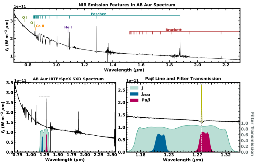
Figure 1: Upper Panel: A mapping of the location of emission lines in the NIR IRTF spectrum of AB Aur A. Lower Left: The entire flux-calibrated IRTF/SpeX SXD spectrum of AB Aur A (Section 2.2). The spectral ranges $\approx$1.3–1.5 $\mu$m and $\approx$1.7–1.9 $\mu$m fall in telluric regions and have reduced signal to noise. The grey dotted box indicates the spectral region containing the Pa$\beta$ line and the NIRC2 filter bandpasses utilized in this work. Lower Right: A zoomed-in perspective of the region within the dotted box in the left panel. The light green emission component of the Pa$\beta$ line indicates the region that was masked during our calculation of the host star’s synthetic J_cont magnitude ($J_{cont,syn}$). The transmission profiles of the relevant NIRC2 filters are displayed below (J filter is shown in teal, the J_cont filter is shown in blue, and the Pa$\beta$ filter is shown in red). The vertical dashed line traces Pa$\beta$ emission line location.

Table 1: Emission Lines in the IRTF/SpeX NIR Spectrum of AB Aur.

Line ID	$\lambda_{obs}$	EW	$\sigma_{\mathrm{EW}}$
	($\mu$m)	(Å)	(Å)
O I	0.7776	-0.33	0.06
O I + H I (18–3)	0.8451	-0.62	0.05
Ca II + H I (15–3)	0.8546	-0.97	0.05
H I (14–3)	0.8603	-0.09	0.03
Ca II + H I (13–3)	0.8668	-0.32	0.04
H I (12–3)	0.8754	-0.18	0.03
H I (11–3)	0.8867	-0.36	0.03
H I (10–3)	0.9019	-0.42	0.03
H I (9–3)	0.9233	-0.89	0.04
H I (8–3) Pa$\epsilon$	0.955	-1.51	0.06
H I (7–3) Pa$\delta$	1.0054	-2.96	0.05
He I $\lambda$1.0830 $\mu$m	1.0837a	-2.40	0.06
H I (6–3) Pa$\gamma$	1.0944	-5.58	0.08
H I (5–3) Pa$\beta$	1.2824	-11.58	0.09
H I (19–4)	1.5268	-0.17	0.05
H I (18–4)	1.5349	-0.22	0.05
H I (17–4)	1.5444	-0.24	0.05
H I (16–4)	1.5565	-0.19	0.05
H I (15–4)	1.5708	-0.16	0.04
H I (14–4)	1.5888	-0.42	0.05
H I (13–4)	1.6116	-0.51	0.06
H I (12–4)	1.6414	-0.50	0.06
H I (11–4)	1.6814	-0.62	0.07
H I (10–4)	1.7369	-0.82	0.09
H I (4–3)	1.8759	-21.41	3.71
H I (7–4) Br$\gamma$	2.1663	-3.28	0.13

Note. — ^aThe He I $\lambda$1.0830$\mu$m line exhibits a clear P-Cygni shape, and the reported $\lambda_{obs}$ signifies the location of the peak of the emission component only.

Figure 2: Left 6 Panels: Normalized quality maps based on injection-recovery tests for the movement and annuli parameters of the KLIP processing using 20 principle components. From upper-left to lower-right, the metrics presented are: mean S/N, maximum S/N, average contrast, mean S/N nearest neighbor, max S/N nearest neighbor, and false-positive fraction. See Section 3.1 for details. Individual maps are normalized and colored according to the respective quality rating (0=worst quality, 1=best quality). These quality metric maps are used to compute the aggregate quality map from which the optimal parameter combinations are chosen. Right Panel: The aggregate quality map constructed from the equally weighted summation of all 6 quality metric maps. The cell with the highest rating from the aggregate map is outlined in black in every panel. Cells containing no quality rating have a combination of movement and annuli parameters that leave no reference images for PSF subtraction as a result of the aggressiveness of the rotational mask.

3 Results

3.1 PSF Subtraction

We performed PSF subtraction on the 50 long-exposure Pa$\beta$ images from the ADI sequence with pyKLIP software (Wang et al., 2015). The KLIP parameters used to produce the PSF-subtracted image were selected according to a data-driven approach inspired by the “pyKLIP Parameter Explorer” algorithm (pyKLIP-PE) developed by Adams Redai et al. (2023), whereby the most optimal KLIP parameters are identified based on several image quality metrics describing the effectiveness of PSF subtraction in an injection-recovery analysis. The primary advantage of this data-driven approach is that it ensures the procedure for PSF subtraction does not rely on a prior significant point source detection and reduces cognitive biases in parameter selection (e.g., Follette et al. 2022; Adams Redai et al. 2023).

Our approach aims at optimizing the following parameters that were found by Follette et al. (2022) and Adams Redai et al. (2023) to have the greatest impact on PSF subtraction with pyKLIP: numbasis (the number of principal components used to construct the PSF), movement (the minimum number of pixels through which a planet will have rotated between the target and reference images), and annuli (the number of concentric and equal-width annular zones that are analyzed independently by pyKLIP).

The procedure for our adopted algorithm is as follows:

1. We first inject several synthetic planets into the pre-processed images at PAs increasing sequentially by 85$\arcdeg$ and radial separations of one FWHM (4.5 pix, or 0.044^′′), beginning at a separation of 0.2^′′ outward to 0.75^′′. Each synthetic planet is assigned a flux of 7 times the standard deviation of the local image background; a value slightly greater than the 5$\sigma$ detection threshold, which allows a range of parameter combinations to be tested that will still result in a robust detection.

2. Next, an individual KLIP reduction is performed for every combination of input parameters numbasis = [5, 10, 15, 20, 25, 30], movement = [1, 2, …, 24, 25], and annuli = [1, 2, …, 24, 25], probing a range of aggressive and conservative permutations of PSF subtraction. The parameters held constant across all reductions are the inner working angle (IWA=20 pixels), and the number of subsections used to divide the annular zones (subsections=1).

3. Then, the point source detection sensitivity for each combination of parameters is represented as a combination of six quality metrics that are determined based on the recovered properties of the synthetic planets. The quality metrics are:

   • The average recovered S/N of the injected planets.

   • The maximum recovered S/N of the injected planets.

   • The average recovered contrast of the injected planets.

   • The “false positive fraction” of the image pixels—the fraction of pixels with a S/N $>$5$\sigma$ within an annulus at the injected planet’s separation with thickness $\Delta r$ = 5 pix, or 0.048^′′ (slightly larger than the FWHM of 4.5 pix, to ensure all necessary pixels are counted). The regions containing the candidate and injected planets are first masked before determining this false positive fraction.

   • The final two “neighbor quality” metrics represent the average and maximum S/N metric values listed above. The neighbor quality metrics are obtained by smoothing the average and maximum S/N in movement/annuli space for each KL parameter “slice”. Neighbor quality metrics are an important consideration because small variations between KLIP parameters should not heavily affect the S/N recovered from a real planet. Smoothing will therefore penalize combinations of movement and annuli parameters that produce drastic variations in S/N among neighboring cells.

The final selection of movement and annuli, output metrics that were computed for numbasis = 5, and numbasis = 30 are averaged, normalized to unity, and summed to produce a single “aggregate quality map” (Figure 2). The cell containing the highest aggregate quality metric (a maximum possible value of 6) yields the combination of movement and annuli parameters that is optimal, assuming equal weights for each metric in this framework. For this Pa$\beta$ dataset, the best values are movement=4 and annuli=5.

To determine the final numbasis component, we repeat this process without averaging any numbasis slices, now producing six aggregate quality maps—one for each principle component that we tested. The optimal numbasis is that which corresponds to the aggregate quality map with the highest metric corresponding to movement=4 and annuli=5, which we determine to be numbasis=20. Ultimately, the final set of the KLIP parameters that produce the highest quality PSF-subtracted image (Figure 3) is movement=4, annuli=5, and numbasis=20.

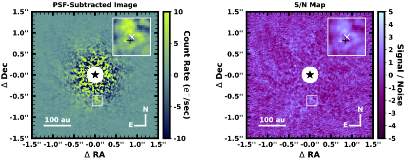
Figure 3: Left: The PSF-subtracted image of AB Aur produced with optimized pyKLIP processing parameters (Section 3.1). Right: The S/N map of the PSF-subtracted image where the S/N of each pixel is computed as the flux divided by the standard deviation of the background in a narrow annulus at that pixel’s separation. The inset frame in the upper right portion of both panels provides an enlarged perspective of the region outlined by the white box at the expected location of the companion. Within the inset views, the white “$\times$” indicates the most recent location reported by Currie et al. (2022) (sep = 0.60^′′, PA = 184.2$\arcdeg$), and the black “+” gives the location reported by Zhou et al. (2022) (sep = 0.60^′′, PA = 182.5$\arcdeg$). The S/N within an aperture radius of 3$\times$FWHM at the position of the white “$\times$” is 1.4, and the S/N at the position of the black “+” is 0.8, both of which are below our threshold of 5$\sigma$ that we use to establish a reliable detection.

3.2 Characterizing Detection Sensitivity in Pa$\beta$

We conducted injection-recovery tests to quantify the throughput of the KLIP reduction results and calibrate the 5$\sigma$ Pa$\beta$ contrast. Because AB Aur b has been spatially resolved in previous detections (e.g., Currie et al. 2022; Zhou et al. 2023), we perform the injection-recovery test for spatially resolved sources. We also perform the nominal test for unresolved sources to quantify throughput of all potential companions in the field. For both cases, synthetic planets are injected over a series of PAs spaced by 40$\arcdeg$, avoiding overlap with the expected PA of AB Aur b ($\approx$180$\arcdeg$). For the spatially resolved case, we construct the template of the injected profile by convolving a 2-dimensional Gaussian kernel with a FWHM equal to the NIRC2 angular resolution at 1.29 $\mu$m (0.044^′′) with with a flat circle with a radius equal to the intrinsic radius of AB Aur b’s spatial profile of $\approx$0.045^′′ (Currie et al., 2022). The resulting profile is a spatially extended source with a FWHM = 0.086^′′.

We injected the spatially extended source at radial separations equally spaced by 2$\times$FWHM of the injected profile, and each profile was scaled to a peak flux equal to 15 times the standard deviation of the noise within an annulus 1-pixel wide at that planet’s separation. These fluxes ensure that the throughput is calculated accurately in post-processing with minimal effects from artifacts that can be created by bright synthetic planets. The throughput was then computed from the average ratio of the injected and recovered fluxes. Then, the S/N map of the PSF-subtracted image was constructed, first masking out a circular region 2$\times$FWHM in diameter centered on the expected location of the companion. For each pixel, we measure the flux in an aperture with a diameter equal to twice the FWHM of the PSF. Next, the aperture-integrated flux was divided by the standard deviation of the fluxes in an annulus covering the remaining azimuthal region, producing a map of the S/N for every pixel in the image (Figure 3). We then derived an initial 5$\sigma$ contrast curve of the post-processed image by calibrating the deep images with unsaturated Pa$\beta$ frames. The location of the candidate was masked during this process, and the $t$-distribution correction was applied to account for small number statistics close to the inner working angle (Mawet et al., 2014). The throughput-corrected 5$\sigma$ contrast curve was computed by dividing the uncorrected contrast value at each resolution element with the throughput at the nearest separation. Figure 4 shows the resulting Pa$\beta$ contrast achieved at separations out to $\approx$2.5^′′ with tabulated values of separation vs Pa$\beta$ contrast given in Appendix A.

3.3 No Detection of Pa$\beta$ Emission

The S/N map of the PSF-subtracted image reveals neither a clear spatially resolved source nor an unresolved source with a S/N ratio at the 5$\sigma$ detection threshold anywhere in the 2$\farcs$5 $\times$ 2$\farcs$5 FOV surrounding the star. At the expected location of AB Aur b corresponding to the epoch reported by Currie et al. (2022) (UT 2020 October 12: sep = 0.599^′′ $\pm$ 0.005^′′, PA = 184.2 $\pm$ 0.6$\arcdeg$), the S/N = 1.4. At the location corresponding to the epoch reported by Zhou et al. (2022) (UT 2022 March 28: sep = 0.600^′′ $\pm$ 0.022^′′, PA = 182.5 $\pm$ 1.4$\arcdeg$), the S/N = 0.8. We therefore do not detect emission in Pa$\beta$ from AB Aur b. At a separation of 0.6^′′, the achieved contrast $\Delta$Pa$\beta$ for a spatially resolved source is 9.6 mag (9.8 mag for an unresolved source). Figure 5 shows four synthetic sources (both resolved and unresolved), injected into the image with fluxes equal to their respective 5$\sigma$ confidence level with separations 0.4^′′, 0.6^′′, 0.8^′′ and 1.0^′′ at PA = 270$\arcdeg$. Each synthetic source is readily visible, and no other comparably bright features are evident elsewhere in the image. Although the continuum contrast between AB Aur b and its host star is lower, $\Delta J$ $\approx$ 9.2 mag (Currie et al., 2022), the host star is accreting and exhibits strong emission in Pa$\beta$  which will impact the contrast in this narrow band filter of the companion, and may explain why the companion was not recovered.

We also note an apparent region of elevated intensity near the expected location of AB Aur b (Figure 3). The region appears to be spatially extended with peak intensity occurring at PA and separation of 184.0$\arcdeg$ and 0.55^′′. The PA is similar to the nominal location of AB Aur b, yet its separation is smaller than the expected separation of the protoplanet. The peak S/N in the region is 4.0, which remains below the 5$\sigma$ detection threshold. Deeper Pa$\beta$ observations could help clarify whether this is extended source is real and associated with AB Aur b.

Figure 4: The 5$\sigma$ contrast curve of the PSF-subtracted image of AB Aur in the NIRC2 narrow band Pa$\beta$ filter computed for an unresolved source (pink) and a resolved source (maroon). Although the expected $\Delta$J contrast is $\approx$9.2 (Currie et al., 2022), the relative Pa$\beta$ emission line strength between the accreting host star and the candidate companion will impact the contrast of the companion in the Pa$\beta$ filter.

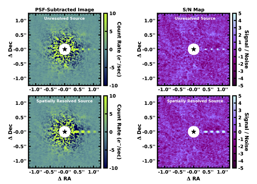
Figure 5: The PSF-Subtracted Image (left column) and corresponding S/N Map (right column) showing several 5$\sigma$ injected sources that are unresolved (top row) and spatially resolved (bottom row). The synthetic sources are located at PA = 270$\arcdeg$ with separations 0.4^′′, 0.6^′′, 0.8^′′, and 1.0^′′. The FOV is slightly smaller than that in Figure 3 for enhanced visual clarity.

3.4 Monochromatic Pa$\beta$ Flux Density of AB Aur b

We compute an upper limit on the monochromatic flux density of AB Aur b from the upper limit of the apparent magnitude in Pa$\beta$. Typically, this is determined using the apparent magnitude of the central star to calibrate the 5$\sigma$ contrast achieved at the expected separation of the companion:

$$Pa\beta_{\textrm{b}}=\Delta Pa\beta+Pa\beta_{\textrm{A}}$$ (1)

where $\Delta$Pa$\beta$ is the contrast at the separation of the companion, and Pa$\beta_{A}$ is the apparent magnitude of the host star in Pa$\beta$. AB Aur has a strong Pa$\beta$ emission line, which may vary over time, so the apparent magnitude of the host star in that bandpass during the observations is not known. To recover Pa$\beta_{A}$ during the long-exposure images used in the high-contrast imaging sequence, we utilize the following relation,

$$Pa\beta_{\textrm{A}}=J_{cont,syn}-(J_{cont}-Pa\beta).$$ (2)

Here, $J_{cont,syn}$ is a synthetic J_cont magnitude of AB Aur A, which we derived from our flux-calibrated IRTF spectrum, and the (J_cont–Pa$\beta$) color is a single quantity denoting the stellar J_cont–Pa$\beta$ color measured from the short-exposure (unsaturated) NIRC2 image sequences taken close together in time (within a 10 min time frame) immediately prior to the long-exposure ADI sequence. This method for obtaining Pa$\beta_{A}$ assumes that AB Aur A’s continuum in $J$ is constant. Long-term NIR monitoring by Shenavrin et al. (2019) shows that the J magnitude of the central star varies by 0.37 mag on timescales of $\approx$1000 days (likely caused by dynamic processes in the inner region of the circumstellar disk; Shenavrin et al. 2019). Furthermore, accretion onto the star could fluctuate, which would vary the emission line strength in the J-band region. For robustness, we adopt this uncertainty into our result for $J_{cont,syn}$.

The IRTF spectrum is flux calibrated by matching the synthetic $J_{MKO}$ filter magnitude to 2MASS J-band photometry (Figure 1). We then performed synthetic photometry using the IRTF spectrum and the NIRC2 J_cont filter profile, returning $J_{cont,syn}$ = 5.96 $\pm$ 0.37 mag.

Next, we calculated the J_cont–Pa$\beta$ color of AB Aur A with the unsaturated J_cont and Pa$\beta$ images. For both filters, the detector counts were summed within a circular aperture centered on the stellar PSF, then divided by the integration times to give count rates in DN s^-1. The aperture radius for J_cont was 2$\times$FWHM, and the radius for Pa$\beta$ was scaled according to the ratio of the central wavelengths of the J_cont and Pa$\beta$ filters. The uncertainty of the total count rate is the standard deviation of that measured for each frame in the associated sequence. This procedure was repeated for the NIRC2 J_cont and Pa$\beta$ images of the A0 star HD 109691 from UT 2023 May 3, which was used to calibrate AB Aur’s J_cont–Pa$\beta$ color to the Vega system as follows:

$$J_{cont}-Pa\beta=-2.5\log_{10}\frac{C_{Jcont}/C_{Pa\beta}}{C^{\textrm{A0}}_{Jcont}/C^{\textrm{A0}}_{Pa\beta}}$$ (3)

where $C_{Jcont}$ and $C_{Pa\beta}$ are the measured detector count rates of AB Aur in each filter and $C^{\textrm{A0}}_{Jcont}$ and $C^{\textrm{A0}}_{Pa\beta}$ are the count rates measured for an A0 star in each filter. The count ratio $C^{\textrm{A0}}_{Jcont}/C^{\textrm{A0}}_{Pa\beta}$ is effectively the color of Vega (or any other A0V star) modulated by wavelength-dependent throughput losses from the atmosphere, telescope, filters, and detector. Using Equation 3, we find a color of J_cont–Pa$\beta$ = 0.16 $\pm$ 0.26 mag.

Using our results for $J_{cont,syn}$ and J_cont–Pa$\beta$, the Pa$\beta$ apparent magnitude of the star is Pa$\beta_{A}$ = 5.80 $\pm$ 0.44 mag at the time of our observations. In conjunction with the achieved contrast at 0.6^′′ separation ($\Delta$Pa$\beta$ = 9.6 mag for the resolved case, $\Delta$Pa$\beta$ = 9.8 mag for the unresolved case; Section 3.2), the 5$\sigma$ lower limit on the apparent magnitude of a spatially resolved AB Aur b is Pa$\beta_{b}$ $>$ 15.40 $\pm$ 0.44 mag (15.60 $\pm$ 0.44 mag for the unresolved scenario). Applying a synthetic Vega Pa$\beta$ zero-point $f^{\textrm{Vega}}_{Pa\beta}$ = 2.50$\times$10^-9 W m^-2 $\mu$m^-1, which was obtained with the Vega spectrum built into pysynphot, the associated monochromatic flux density is $f_{Pa\beta}\leq$ 1.73 $\pm$ 0.71$\times$10^-15 W m${}^{-2}~{}\mu$m^-1 (1.44 $\pm$ 0.59$\times$10^-15 W m${}^{-2}~{}\mu$m^-1, unresolved). We proceed with a conservative treatment of $f_{Pa\beta}$, and adopt a hard upper limit equal to 2$\sigma$ above the mean value: henceforth, $f_{Pa\beta}\leq$ 3.14$\times$10^-15 W m${}^{-2}~{}\mu$m^-1 (2.61$\times$10^-15 W m${}^{-2}~{}\mu$m^-1, unresolved; Figure 6).

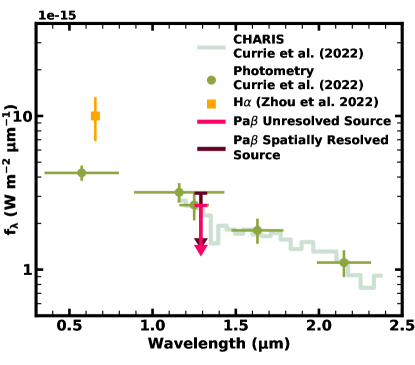
Figure 6: SED of AB Aur b. The adopted upper limit of the flux density in Pa$\beta$ for an unresolved source is indicated by the pink downward-pointing arrow, whereas the upper limit of the flux density for a spatially resolved source is shown depicted as a maroon arrow. The green circles are the optical (HST) and NIR (Subaru) photometry reported by Currie et al. (2022), and the CHARIS spectrum they report is represented in light-green. The orange square point indicates the H$\alpha$ excess identified by Zhou et al. (2022) with HST.

3.5 Pa$\beta$ Equivalent Width

To estimate the central star’s EW at the time of imaging, we masked the Pa$\beta$ emission line flux in the IRTF/SpeX SXD spectrum, and replaced the missing flux with a series of artificial emission lines with amplitudes ranging from –1 to 14 times the flux of the continuum at the line center, increasing sequentially by factors of 0.1. Each line is assigned a width corresponding to the SXD resolving power of $\approx$0.0006 $\mu$m. Next, the EW is calculated individually for each line and then mapped to the synthetic stellar J_cont–Pa$\beta$ derived from the IRTF spectrum containing the corresponding simulated emission line. The true EW of the stellar Pa$\beta$ emission line is then inferred from the simulated J_cont–Pa$\beta$ color that matches the observed value (J_cont–Pa$\beta$ = 0.16 $\pm$ 0.26 mag; Figure 7). The results of this test indicate that the EW of the stellar Pa$\beta$ line at the time of the imaging sequence is –94 $\pm$ 64 Å. The EW of the Pa$\beta$ emission line in the IRTF spectrum obtained $\sim$8 days later is $-11.58\,\pm\,0.09$ Å (Table 1).

Figure 7: EWs and stellar color and companion flux density corresponding to simulated Pa$\beta$ emission lines injected into the stellar continuum (top) and companion continuum (bottom). The solid grey line in the top panel indicates the real measured stellar J_cont–Pa$\beta$ and the shaded region bounded by dashed lines represents the 1$\sigma$ uncertainty on the measurement. The green star marks the simulated quantity that matches the observed stellar J_cont–Pa$\beta$. The bottom panel shows the EW estimations for both an unresolved source and spatially resolved source. The uppermost boundary of each of the shaded regions indicates the upper limit of the companion flux density determined in Section 3.4. The pink and maroon stars mark the simulated quantities that match the measured upper limits on the companion’s flux density if it were unresolved or resolved, respectively. EW values are negative for emission lines.

We obtained the companion’s maximum detectable Pa$\beta$ emission line strength with similar methods. We injected synthetic emission line profiles are into the CHARIS near-infrared spectrum of AB Aur b from Currie et al. (2022) following the same prescription for line amplitude and width as was done for the central star. The EW of each simulated emission line was mapped to the corresponding flux density of the continuum-plus-emission line through the NIRC2 Pa$\beta$ filter. Using this empirical relationship between Pa$\beta$ flux density and EW (Fig 7), we determine that AB Aur b’s flux density upper limit $f_{\textrm{Pa}\beta}\leq$ 3.14$\times$10^-15 W m${}^{-2}~{}\mu$m^-1 (2.61$\times$10^-15 W m${}^{-2}~{}\mu$m^-1, unresolved) corresponds to a lower limit in its EW of –54 Å (–11 Å, unresolved). A significant difference in strength of the Pa$\beta$ emission line between the star and the companion would be evidence that the companion is self-luminous (i.e., a protoplanet). However, their EWs agree at the 0.64$\sigma$ and 1.3$\sigma$ level for the spatially resolved and unresolved cases, respectively, offering no evidence of a significant ($\geq$3$\sigma$) discrepancy in Pa$\beta$ emission. This is consistent with both the light-scattering scenario as well as the scenario in which a young planet is weakly accreting.

4 Discussion

Our deep Pa$\beta$ imaging does not reveal excess emission from AB Aur b, nor any other point source in the system. There is some tension between our upper limits at the location of the planet and the nominal published J-band continuum level of AB Aur b. As described in Section 3.4, the 5$\sigma$ contrast level corresponds to an upper limit of 1.73 $\pm$ 0.71$\times$10^-15 W m${}^{-2}~{}\mu$m^-1 assuming a spatially resolved source (or 1.44 $\pm$ 0.59$\times$10^-15 W m${}^{-2}~{}\mu$m^-1 for the unresolved case in which AB Aur b is a point source), which is below the continuum emission reported by Currie et al. (2022) at this wavelength. But as there is an uncertainty associated with our upper limit, we have conservatively adopted the 95% upper bound on this value to guard against potential systematic errors in the multi-step process of converting contrast measurements into a flux density within this narrow-band filter.

There are a few potential explanations that can account for the companion flux being undetectable at the published continuum level:

• If we consider the companion to be a self-luminous protoplanet, we can rule out strong Pa$\beta$ emission, implying weak accretion or no accretion at all from the companion.

• Alternatively, if the companion’s emission source is a compact protoplanetary disk feature seen in scattered starlight, one or both of the following may be possible. The localized dynamics in the disk material could have changed the effective light-scattering area of the disk substructure (e.g., LkCa 15 Thalmann et al. 2016; Currie et al. 2019; Sallum et al. 2023). Alternatively, there could have been enhanced Pa$\beta$ emission caused by accretion onto the central star, but the delay in light travel time to reach the companion may have prevented the observation of enhanced emission at the location of AB Aur b within the observing window.

• Finally, irrespective of the true nature of the emission source, the following two possibilities could also contribute to this modest tension: the J-band region is known to be moderately variable at the 0.4 mag level (Shenavrin et al., 2019), and could have affected the continuum flux calibration (see also Section 3.4).

• Alternatively, the absolute calibration level of the CHARIS continuum may be inaccurate. For this analysis, we have assumed that the companion’s continuum is both constant and accurate.

5 Summary

In this work, we obtained high-contrast imaging of AB Aur with Keck/NIRC2 in the Pa$\beta$ narrow-band filter. We do not detect significant Pa$\beta$ emission in the FOV surrounding the star, either from AB Aur b or any other potential embedded planets. However, the depth of our observations place a meaningful upper limit on the Pa$\beta$ line flux. Mapping this flux to its associated EW, we find that, if present, Pa$\beta$ emission is weak. However, we cannot conclude whether it must be significantly weaker in comparison to emission from the central star at the time of the observations, which would have provided a direct test of the scattered light versus self-luminous hypothesis because the line-to-continuum ratio is expected to differ in the latter scenario. Deeper Pa$\beta$ imaging, NIR spectroscopy, and multi-wavelength observations of AB Aur b will help clarify the nature of this enigmatic source.

Appendix A Pa$\beta$ Contrast Curve

Table 2: Separation vs. Pa$\beta$ contrast (Figure 4) achieved in our high-contrast imaging of AB Aur.

Separation	Spatially Resolved	Unresolved
(′′)	Contrast ($\Delta$mag)	Contrast ($\Delta$mag)
0.26	-5.22	-6.48
0.32	-5.93	-7.46
0.39	-7.54	-8.21
0.45	-8.07	-8.75
0.52	-8.71	-9.46
0.58	-9.58	-9.84
0.65	-9.83	-10.13
0.71	-10.27	-10.41
0.78	-10.53	-10.69
0.84	-10.78	-10.95
0.91	-10.99	-11.2
0.97	-11.17	-11.39
1.04	-11.31	-11.53
1.1	-11.52	-11.67
1.17	-11.57	-11.76
1.23	-11.69	-11.82
1.3	-11.74	-11.85
1.36	-11.75	-11.87
1.43	-11.82	-11.9
1.49	-11.83	-11.91
1.56	-11.8	-11.92
1.62	-11.82	-11.94
1.69	-11.83	-11.96
1.75	-11.89	-12
1.82	-11.92	-12.02
1.88	-11.94	-12.05
1.95	-11.99	-12.08
2.01	-12	-12.09
2.08	-12.01	-12.08
2.14	-12.01	-12.07
2.21	-11.98	-12.05
2.27	-11.99	-12.07
2.34	-11.99	-12.08
2.4	-12	-12.09
2.47	-11.96	-12.05

References

- Adams Redai et al. (2023) Adams Redai, J. I., Follette, K. B., Wang, J., et al. 2023, AJ, 165, 57, doi: 10.3847/1538-3881/aca60d
- Aoyama et al. (2018) Aoyama, Y., Ikoma, M., & Tanigawa, T. 2018, ApJ, 866, 84, doi: 10.3847/1538-4357/aadc11
- Aoyama et al. (2020) Aoyama, Y., Marleau, G.-D., Mordasini, C., & Ikoma, M. 2020, arXiv e-prints, arXiv:2011.06608, doi: 10.48550/arXiv.2011.06608
- Biller et al. (2014) Biller, B. A., Males, J., Rodigas, T., et al. 2014, ApJ, 792, L22, doi: 10.1088/2041-8205/792/1/L22
- Bowler et al. (2011) Bowler, B. P., Liu, M. C., Kraus, A. L., Mann, A. W., & Ireland, M. J. 2011, ApJ, 743, 148, doi: 10.1088/0004-637X/743/2/148
- Choksi & Chiang (2022) Choksi, N., & Chiang, E. 2022, MNRAS, 510, 1657, doi: 10.1093/mnras/stab3503
- Costigan et al. (2014) Costigan, G., Vink, J. S., Scholz, A., Ray, T., & Testi, L. 2014, MNRAS, 440, 3444, doi: 10.1093/mnras/stu529
- Currie et al. (2019) Currie, T., Marois, C., Cieza, L., et al. 2019, ApJ, 877, L3, doi: 10.3847/2041-8213/ab1b42
- Currie et al. (2022) Currie, T., Lawson, K., Schneider, G., et al. 2022, Nature Astronomy, 6, 751, doi: 10.1038/s41550-022-01634-x
- Cushing et al. (2004) Cushing, M. C., Vacca, W. D., & Rayner, J. T. 2004, PASP, 116, 362, doi: 10.1086/382907
- Demars et al. (2023) Demars, D., Bonnefoy, M., Dougados, C., et al. 2023, arXiv e-prints, arXiv:2305.09460. https://arxiv.org/abs/2305.09460
- Follette et al. (2017) Follette, K. B., Rameau, J., Dong, R., et al. 2017, AJ, 153, 264, doi: 10.3847/1538-3881/aa6d85
- Follette et al. (2022) Follette, K. B., Close, L. M., Males, J. R., et al. 2022, arXiv e-prints, arXiv:2211.02109, doi: 10.48550/arXiv.2211.02109
- Fruchter & Hook (2002) Fruchter, A. S., & Hook, R. N. 2002, PASP, 114, 144, doi: 10.1086/338393
- Gaia Collaboration (2020) Gaia Collaboration. 2020, VizieR Online Data Catalog, I/350
- Guzmán-Díaz et al. (2021) Guzmán-Díaz, J., Mendigutía, I., Montesinos, B., et al. 2021, A&A, 650, A182, doi: 10.1051/0004-6361/202039519
- Haffert et al. (2019) Haffert, S. Y., Bohn, A. J., de Boer, J., et al. 2019, Nature Astronomy, 3, 749, doi: 10.1038/s41550-019-0780-5
- Harrington & Kuhn (2007) Harrington, D. M., & Kuhn, J. R. 2007, ApJ, 667, L89, doi: 10.1086/521999
- Hunter (2007) Hunter, J. D. 2007, Computing in Science & Engineering, 9, 90, doi: 10.1109/MCSE.2007.55
- Keppler et al. (2018) Keppler, M., Benisty, M., Müller, A., et al. 2018, A&A, 617, A44, doi: 10.1051/0004-6361/201832957
- Ligi et al. (2018) Ligi, R., Vigan, A., Gratton, R., et al. 2018, MNRAS, 473, 1774, doi: 10.1093/mnras/stx2318
- Lim et al. (2013) Lim, P. L., Diaz, R. I., & Laidler, V. 2013, pysynphot: Synthetic photometry software package, Astrophysics Source Code Library, record ascl:1303.023. http://ascl.net/1303.023
- Liu (2004) Liu, M. C. 2004, Science, 305, 1442, doi: 10.1126/science.1102929
- Marleau & Aoyama (2022) Marleau, G.-D., & Aoyama, Y. 2022, Research Notes of the American Astronomical Society, 6, 262, doi: 10.3847/2515-5172/acaa34
- Marois et al. (2006) Marois, C., Lafrenière, D., Doyon, R., Macintosh, B., & Nadeau, D. 2006, ApJ, 641, 556, doi: 10.1086/500401
- Mawet et al. (2014) Mawet, D., Milli, J., Wahhaj, Z., et al. 2014, ApJ, 792, 97, doi: 10.1088/0004-637X/792/2/97
- Mendigutía et al. (2018) Mendigutía, I., Oudmaijer, R. D., Schneider, P. C., et al. 2018, A&A, 618, L9, doi: 10.1051/0004-6361/201834233
- Pohl et al. (2017) Pohl, A., Benisty, M., Pinilla, P., et al. 2017, ApJ, 850, 52, doi: 10.3847/1538-4357/aa94c2
- Rameau et al. (2017) Rameau, J., Follette, K. B., Pueyo, L., et al. 2017, AJ, 153, 244, doi: 10.3847/1538-3881/aa6cae
- Rayner et al. (2003) Rayner, J. T., Toomey, D. W., Onaka, P. M., et al. 2003, PASP, 115, 362, doi: 10.1086/367745
- Robitaille et al. (2021) Robitaille, T., Tollerud, E., Aldcroft, T., et al. 2021, astropy/astropy: v4.2.1, v4.2.1, Zenodo, Zenodo, doi: 10.5281/zenodo.4670729
- Sallum et al. (2023) Sallum, S., Eisner, J., Skemer, A., & Murray-Clay, R. 2023, ApJ, 953, 55, doi: 10.3847/1538-4357/ace16c
- Santamaría-Miranda et al. (2018) Santamaría-Miranda, A., Cáceres, C., Schreiber, M. R., et al. 2018, MNRAS, 475, 2994, doi: 10.1093/mnras/stx3325
- Schmidt et al. (2008) Schmidt, T. O. B., Neuhäuser, R., Seifahrt, A., et al. 2008, A&A, 491, 311, doi: 10.1051/0004-6361:20078840
- Seifahrt et al. (2007) Seifahrt, A., Neuhäuser, R., & Hauschildt, P. H. 2007, A&A, 463, 309, doi: 10.1051/0004-6361:20066463
- Service et al. (2016) Service, M., Lu, J. R., Campbell, R., et al. 2016, PASP, 128, 095004, doi: 10.1088/1538-3873/128/967/095004
- Shenavrin et al. (2019) Shenavrin, V. I., Grinin, V. P., Baluev, R. V., & Demidova, T. V. 2019, Astronomy Reports, 63, 1035, doi: 10.1134/S1063772919120060
- Sissa et al. (2018) Sissa, E., Gratton, R., Garufi, A., et al. 2018, A&A, 619, A160, doi: 10.1051/0004-6361/201732332
- Stolker et al. (2021) Stolker, T., Haffert, S. Y., Kesseli, A. Y., et al. 2021, AJ, 162, 286, doi: 10.3847/1538-3881/ac2c7f
- Szulágyi & Ercolano (2020) Szulágyi, J., & Ercolano, B. 2020, ApJ, 902, 126, doi: 10.3847/1538-4357/abb5a2
- Szulágyi et al. (2014) Szulágyi, J., Morbidelli, A., Crida, A., & Masset, F. 2014, ApJ, 782, 65, doi: 10.1088/0004-637X/782/2/65
- Tang et al. (2017) Tang, Y.-W., Guilloteau, S., Dutrey, A., et al. 2017, ApJ, 840, 32, doi: 10.3847/1538-4357/aa6af7
- Tanigawa et al. (2012) Tanigawa, T., Ohtsuki, K., & Machida, M. N. 2012, ApJ, 747, 47, doi: 10.1088/0004-637X/747/1/47
- Thalmann et al. (2016) Thalmann, C., Janson, M., Garufi, A., et al. 2016, ApJ, 828, L17, doi: 10.3847/2041-8205/828/2/L17
- Thanathibodee et al. (2019) Thanathibodee, T., Calvet, N., Bae, J., Muzerolle, J., & Hernández, R. F. 2019, ApJ, 885, 94, doi: 10.3847/1538-4357/ab44c1
- van Holstein et al. (2021) van Holstein, R. G., Stolker, T., Jensen-Clem, R., et al. 2021, A&A, 647, A21, doi: 10.1051/0004-6361/202039290
- vanderWalt2011 et al. (2011) vanderWalt2011, S., Colbert, S. C., & Varoquaux, G. 2011, Computing in Science & Engineering, 13, 22, doi: 10.1109/MCSE.2011.37
- Virtanen et al. (2021) Virtanen, P., Gommers, R., Burovski, E., et al. 2021, scipy/scipy: SciPy 1.6.3, v1.6.3, Zenodo, Zenodo, doi: 10.5281/zenodo.4718897
- Wagner et al. (2018) Wagner, K., Follete, K. B., Close, L. M., et al. 2018, ApJ, 863, L8, doi: 10.3847/2041-8213/aad695
- Wang et al. (2015) Wang, J. J., Ruffio, J.-B., De Rosa, R. J., et al. 2015, pyKLIP: PSF Subtraction for Exoplanets and Disks, Astrophysics Source Code Library, record ascl:1506.001. http://ascl.net/1506.001
- Wizinowich et al. (2000) Wizinowich, P., Acton, D. S., Shelton, C., et al. 2000, PASP, 112, 315, doi: 10.1086/316543
- Zhou et al. (2014) Zhou, Y., Herczeg, G. J., Kraus, A. L., Metchev, S., & Cruz, K. L. 2014, ApJ, 783, L17, doi: 10.1088/2041-8205/783/1/L17
- Zhou et al. (2022) Zhou, Y., Sanghi, A., Bowler, B. P., et al. 2022, ApJ, 934, L13, doi: 10.3847/2041-8213/ac7fef
- Zhou et al. (2023) Zhou, Y., Bowler, B. P., Yang, H., et al. 2023, arXiv e-prints, arXiv:2308.16223, doi: 10.48550/arXiv.2308.16223