Triple-Encoders: Representations That Fire Together, Wire Together

Abstract

Search-based dialog models typically re-encode the dialog history at every turn, incurring high cost. Curved Contrastive Learning, a representation learning method that encodes relative distances between utterances into the embedding space via a bi-encoder, has recently shown promising results for dialog modeling at far superior efficiency. While high efficiency is achieved through independently encoding utterances, this ignores the importance of contextualization. To overcome this issue, this study introduces triple-encoders, which efficiently compute distributed utterance mixtures from these independently encoded utterances through a novel hebbian inspired co-occurrence learning objective without using any weights. Empirically, we find that triple-encoders lead to a substantial improvement over bi-encoders, and even to better zero-shot generalization than single-vector representation models without requiring re-encoding. Our code/model is publicly available.

1 Introduction

Traditional search-based approaches in conversational sequence modeling like ConveRT (Henderson et al., 2020) represent the entire context (query) in one context vector (see Figure 1). This has two major drawbacks: (a) Recomputing the entire vector at each turn is computationally expensive, and (b) it is difficult to compress the context’s relevant information for any possible candidate response into a single vector. Furthermore, the encoder models are limited to a maximum number of tokens, usually 512. Curved Contrastive Learning (CCL) (Erker et al., 2023) demonstrated that it is possible to encode utterances separately in a latent space and accumulate sequence likelihood based on solely cosine similarity, thanks to treating cosine similarity not as a semantic but as a directional relative dialog turn distance measure between utterance pairs (through two sub-spaces representing a temporal direction: before and after). This relativistic approach tackles (a), by enabling sequential search with a constant complexity, as only the latest utterance needs to be encoded and computed during inference as shown in Figure 1. (b) Furthermore, each candidate utterance can interact with every independently projected utterance, allowing a richer interaction. However, encoding utterances independently means they are not contextualized, disregarding a crucial feature of conversation as illustrated in Figure 2.

Figure 1: Comparison of our Triple Encoder to Henderson et al. (2020) and Erker et al. (2023). Similar to CCL we only need to encode and compute similarity scores of the latest utterance. At the same time, we achieve contextualization through pairwise mean-pooling with previous encoded utterances combining the advantages of both previous works. Our analysis shows that the co-occurrence training pushes representations that occur (fire) together closer together, leading to stronger additive properties (wiring) when being superimposed (compared to Erker et al. (2023)) and thus to a better next utterance selection.

For the first time, in this paper we propose a method that contextualizes utterance embeddings in dialog sequences in a self-organizing manner, without the use of additional weights, i.e, merely through local interactions (in form of efficient vector algebra) between separately encoded utterances after appropriate pre-training. While previous work has shown that mean pooling is a strong method for sentence composition from tokens (Pagliardini et al., 2018; Reimers and Gurevych, 2019), we demonstrate that this can be generalized to a higher abstraction level: distributed pairwise sequential composition (illustrated in Figure 1). To realize this, we present triple-encoders, which segment the context space of CCL into two distinct latent spaces denoting the relative order of utterances in the context. By linearly combining (averaging) representations from these sub-spaces through a co-occurrence learning objective, we create new contextualized embeddings that we can incorporate into CCL, resulting in Contextualized Curved Contrastive Learning (C3L). At inference time, our method efficiently contextualizes independently encoded utterances based on solely local interactions (without any additional weights): Our method applies only (1) mean pooling, a (2) matrix multiplication for computing the similarity and one (3) summation (across the sequential dimension) operation to aggregate similarity scores. While we focus on modeling dialog in this paper, the sequential modularity of our method can in principle be used for any text sequence. Pilot experiments on next sentence selection of children stories are reported in Appendix F, while we leave thorough exploration to future work.

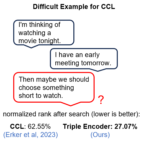
Figure 2: Difficult example for next utterance selection based on solely independent utterances. Here the model must know that both utterances occur together as it requires considering them jointly to derive the third utterance (in red). This is reflected by the significant gap in the normalized rank between our contextualized approach and the uncontextualized approach of Erker et al. (2023).

Our experiments are aimed at the following research questions:

RQ1: What is the effect of triple-encoder training (C3L) + triple encoder at inference compared to CCL?

RQ2: What is the effect of triple-encoder training (C3L) while encoding utterances at inference time without contextualization (like CCL)?

Our experimental results suggest that our approach improves substantially over standard CCL. Notably, our method outperforms ConveRT (Henderson et al., 2020) in a zero-shot setting while our method requires no additional learnable parameters for contextualization. While triple-encoder training alone improves the performance considerably (RQ2), using triple-encoder contextualization at inference time (RQ1) leads to additional performance gains while keeping linear complexity.

2 Related Work

We will start with related work on embedding compositionality, conversational sequence modeling and self-organizing maps. Next, we will describe retrieval methods that have been a motivation to our distributed representations. Lastly, we will discuss CCL as the core foundation of our work.

2.1 Composition and Self-Organization

Weight-less compositionality of embeddings is a well-studied problem for word representations (Mitchell and Lapata, 2008; Rudolph and Giesbrecht, 2010; Mikolov et al., 2013; Mai et al., 2019), but has received little attention for larger text units such as sentences or utterances. For these, investigations are limited to small contexts such as pairwise sentence relations (e.g. NLI) (Sileo et al., 2019) or sentence fusion (Huang et al., 2023), and are outperformed by parameterized composition operators. In the context of conversational sequence modeling, conventional methodologies typically employ parameterized functions (learned weights) that act as an external force to contextualize utterance embeddings that are computed independently (Liu et al., 2022; Zhang et al., 2022). As far as we are aware, this is the first method in which contextualization in conversational sequence modeling has been achieved solely through local interactions, without the reliance on additional weights. This approach aligns with the self-organization principle found in nature that

describes the emergence of global order from local interactions between components of a system without supervision by external directing forces Rezaei-Lotfi et al. (2019)

demonstrating how global order within dialogue sequences can emerge from localized interactions (mean pooling and cosine similarity) among utterance embeddings. The self-organization principle has previously been applied to machine learning in self-organizing maps Kohonen (1982).

2.2 Retrieval

Typically, neural response retrieval systems like ConveRT (Henderson et al., 2020) (see Figure 1) produce a single context embedding per turn that is then compared to candidate utterance embeddings. This leads to weak interactions with candidate utterances as not all information can be compressed into one vector. Previous work in retrieval has addressed the weak interaction of bi-encodings through several techniques. Previous work like MORES (Gao et al., 2020), PreTTR (MacAvaney et al., 2020) or PolyEncoders (Humeau et al., 2020) tackled this problem by encoding each candidate representation with a query via a late-stage self-attention mechanism to enable a richer interaction. Though this technique outperformed traditional bi-encoders, the attention mechanism does not scale with large search spaces. Another technique that was the inspiration for our average and maximum similarity based approaches is ColBERT (Khattab and Zaharia, 2020) and ColBERTV2 (Santhanam et al., 2022) which has shown that this concept works well on word token level.

2.3 Uncontextualized CCL via Bi-Encoder

Figure 3: Concept of relativity in Imaginary Embeddings with $l=5$ using before [B] and after tokens [A] (Erker et al., 2023)

We build upon the previous work on Curved Contrastive Learning (CCL) (Erker et al., 2023), a self-supervised representation learning technique based on sentence embedding methods like SentenceBERT (Reimers and Gurevych, 2019). Similar to how our universe is made up of a stage between space and time, CCL learns a stage between semantics and the directional relative turn distance of utterance pairs in multi-turn dialog. As Figure 3 illustrates, the resulting embeddings are inspired by the concept of relativity (Einstein, 1921): By embedding utterances with special before ([B]) and after ([A]) tokens into two distinct subspaces, directional temporal distances become relative to the observer. Concretely, as Figure 3 shows, when traveling through this space from $t-1$ to the next turn $t$, CCL linearly decreases the similarity to every previous utterance $u_{s},s<t$ and increase the similarity to every $u_{s},s>t$ as part of the sequence. Formally, given a sequence of utterances $u_{0},u_{1},...,u_{n}$, choose a window size $l$, then the pretraining objective of CCL is

$$cos(\operatorname{\mathbf{E}}([B]\ u_{i}),\operatorname{\mathbf{E}}([A]\ u_{k}))=1-\frac{k-i}{l},$$

which we enforce through an MSE loss for $0<k-i<l$. $\operatorname{\mathbf{E}}$ refers to a text encoder such as SBERT. We also refer to this model as the bi-encoder as it uses a dual encoder. This training objective together with directional and random hard negatives shows strong performance in sequence modeling and planning tasks (Erker et al., 2023). While ConveRT encodes $t$ utterances at step $t$, resulting in an overall complexity of $\mathcal{O}(n^{2})$ utterance encodings, this approach only encodes one new utterance at every step, resulting in an overall complexity of $\mathcal{O}(n)$ utterance encodings.

However, we hypothesize that the lack of contextualization does not reflect the dialogs’ highly contextual dependency which prohibits even better performance. With our triple-encoder we address this core limitation as we will show empirically in this paper.

3 Contextualized CCL via Triple-encoders

Figure 4: Our Triple-Encoder architecture with two directional before tokens [B1] and [B2]. We create a combined state of two utterances as the average between the separately encoded embeddings. The target distance of this new combined state results as a normalized sum of each individual utterance score from the bi-encoder Curved Contrastive Learning.

We design an extension to the CCL framework that addresses the aforementioned issue while retaining the same order of encoding complexity at inference as the bi-encoder model ($\mathcal{O}(n)$), resulting in Contextualized Curved Contrastive Learning (C3L).

To enhance the CCL embeddings with contextualization, two additional special tokens are added to the before space, [B1] and [B2]. These tokens denote the relative order of the utterances in the dialog, i.e. $[B1]u_{i}\wedge[B2]u_{j}\Leftrightarrow i<j$ to add positional information. To model the the interaction between these different context utterances, we choose a simple mean operation as shown on the right of Figure 4.

Given that the [B1] and [B2] tokens create distinct representations, they’re effectively projecting the utterance into two different embedding spaces. By combining utterance states of [B1] and [B2] through a mean operation, a new combined state that carries information from both original states is created.

Erker et al. (2023) have shown that the curved scores (a linear decrease of similarity) outperform classic hard positives/negatives in sequence modeling and enhance sequential information that enables better planning capability. To keep the phenomenon of moving in a relativistic fashion through a continuous temporal dimension with respect to the after space, we construct the triple as a joint contribution of its sub-components. Formally, for window size $l$ and $0<i<j<k$ and $k-i<l$, if the distance between $[B1]u_{i}$ and $[A]u_{k}$ is $1-\frac{k-i}{l}$, and the distance between $[B2]u_{j}$ and $[A]u_{k}$ is $1-\frac{k-j}{l}$, then the joint representation of utterances in the before space should have distance $2-\frac{2k-(i+j)}{l}$. Hence, we enforce for positive examples:

$$\begin{split}&\cos\left(\frac{\operatorname{\mathbf{E}}([B1]u_{i})+\operatorname{\mathbf{E}}([B2]u_{j})}{2},\operatorname{\mathbf{E}}([A]u_{k})\right)\\ =&\operatorname{norm}\left(2-\frac{2k-(i+j)}{l}\right),\end{split}$$ (1)

where $\operatorname{norm}$ normalizes the values from $[\frac{1}{l},2-\frac{3}{l}]$ to $[\frac{1}{l},1]$ via min-max scaling to match the range of cosine similarity. Figure 4 illustrates this procedure. Like in CCL, this objective can be computed efficiently when moving from step $t-1$ to $t$, since only the last utterance has to be encoded at every inference step, as Figure 5 illustrates.

3.1 Co-occurence Learning Through Hard Negatives

With the positive training examples from above, the model does not necessarily have to learn co-occurrence information, because it suffices to identify one context utterance in the input to reach a low training error. We introduce hard negative examples to mitigate this. By training every true context representation (both [B1] and [B2]) with one random utterance as hard negatives, we enable a novel co-occurrence learning paradigm that only lets a candidate representation (in the after space) wire to its mixed contextualized representation if both context representations fire in a sequence together. Hard negatives are constructed from random utterances $u_{r},u_{r}^{\prime}$ sampled from the training set:

$$\begin{array}[]{lcl}\cos\left(\frac{\operatorname{\mathbf{E}}([B1]u_{i})+\operatorname{\mathbf{E}}([B2]u_{r})}{2},\operatorname{\mathbf{E}}([A]u_{k})\right)&=&0.0\\ \cos\left(\frac{\operatorname{\mathbf{E}}([B1]u_{r})+\operatorname{\mathbf{E}}([B2]u_{i})}{2},\operatorname{\mathbf{E}}([A]u_{k})\right)&=&0.0\\ \cos\left(\frac{\operatorname{\mathbf{E}}([B1]u_{r})+\operatorname{\mathbf{E}}([B2]u_{r}^{\prime})}{2},\operatorname{\mathbf{E}}([A]u_{k})\right)&=&0.0\\ \end{array}$$ (2)

These are generated for every $1\leq i<k$ and $k-i<l$.

We employ three additional components: First, as a preliminary step, the model is pre-trained as a bi-encoder, i.e., standard CCL. We found this to improve results slightly (Appendix C). Second, we employ the same auxiliary NLI learning objective as is used in standard CCL. Third, like in CCL, we indicate odd and even turns through additional speaker tokens, following (Erker et al., 2023).

Figure 5: Relative time dimension in our proposed Contextual Curved Contrastive Learning. As the observation window moves from $t\rightarrow t+1$, $3$ new triplets are added (dark green), $3$ removed (light green), and $3$ decayed by $-0.4$ (green). As shown through the incoming green arrows at utterance $u_{5}$, we only have to encode the new incoming utterance with a [B2] token. In the next turn we require the [B1] token that can be encoded at idle time while the dialog partner is speaking.

4 Application of Curved Contrastive Learning

This section describes how the bi-encoder and triple-encoder are used after training to solve the two previously introduced tasks (Erker et al., 2023) sequence modeling (Section 4.1) and short-term planning (Section 4.2). Note, when using the triple-encoder as bi-encoder, we use the same setup as CCL bi-encoders.

4.1 Dialog Sequence Modeling

In sequence modeling, given a context prefix $C=u_{1},\dots,u_{k}$ from a dialog $u_{1},\dots,u_{n}$, the task is to find the true utterance $u_{k+1}$ among a set of randomly sampled future utterances. For every candidate utterance $u_{f}\in U_{F}$, the relative likelihood $p(u_{f}|C)$ (similarity score) is computed. For evaluation, we measure the rank of $p(u_{k+1}|C)$ of all utterances in the test corpus at the same depth. The bi-encoder and triple-encoder differ in how $p(u|C)$ is computed.

4.1.1 Bi-Encoder

Following Erker et al. (2023), with the bi-encoder the relative likelihood is computed as the cosine similarity between the candidate utterance and every context utterance (encoded separately) as

$$p(u_{f}|C)=\sum\limits_{u_{i}\in C}cos(\operatorname{\mathbf{E}}([B]u_{i}),\operatorname{\mathbf{E}}([A]u_{f})).$$

While the accumulation is very efficient and worked fairly well, we demonstrate that our triple encoder trained with C3L significantly improves the performance thanks to the extra contextualization.

4.1.2 Triple-Encoder

	B1					Relative	Total
						Growth	States
B2	$u_{1}$	$u_{2}$	$u_{3}$	$u_{4}$	$u_{5}$
$u_{1}$	(X)					0	0
$u_{2}$	1	(X)				1	1
$u_{3}$	2	2	(X)			2	3
$u_{4}$	3	3	3	(X)		3	6
$u_{5}$	4	4	4	4	(X)	4	10

Table 1: Shown are the mean operations between utterances for a sequence length $n=5$. The cell values between [B1] and [B2] indicate the turn in which the relative state is computed. In contrast to the quadratic complexity of ConveRT (Henderson et al., 2020), our model lies within a linear complexity as shown by the number of relative growth.

Similar to the bi-encoder we accumulate the likelihood of a sequence based on the pairwise mixed representations of the entire sequence length $n$. We construct the relative likelihood for every candidate utterance $u_{f}\in U_{F}$ for a context $C:=[u_{1},..,u_{n}]$ of length $n$ as:

As the distributed pairwise mixed representations are superimposed (Equation 3), our embedding space emerges multiple local maxima in the latent space that enables a richer interaction for the candidate (after space) as shown in Figure 1. This stands in stark contrast to traditional search with only one context vector (like ConveRT (Henderson et al., 2020)) where the candidate space is mapped to this one global maximum. This late interaction lets us build upon previous token-based techniques like ColBERT (Khattab and Zaharia, 2020). While Equation 3 effectively captures their averaging approach, in Appendix B we also experiment with their default maximum-based approach, which is 100 times slower than simple averaging in our experimental context.

With our contextualized representations, the number of representations grows to the triangular numbers ($\frac{n(n+1)}{2}$) as shown in the arising triangle of Table 1. However, the relative number of computations at each turn is strictly linear (shown by the relative growth). Therefore at each turn, we simply compute all additional states from $t-1$ to $t$ as one matrix multiplication of size $(|U_{F}|,e\_dim)$ and $(n,e\_dim)^{T}$, where $e\_dim$ denotes the embedding dimension and $|U_{F}|$ the size of the candidate space. Lastly, we add the score matrix of step $n-1$ and rank the candidates in the next step.

As the model is trained only on a fixed window size of $l$, taking the full triangle on longer sequence lengths might lead to unwanted distortions as distances out of this window are not part of the learning objective. Therefore, we also experiment with the $k$ last rows of Table 1. In other words, we here only take the last $k$ utterances in the [B2] space and contextualize them with the entire sequence in the [B1] space with the previously discussed order constraint $[B1]u_{i}\And[B2]u_{j}\Leftrightarrow i<j$. Notably this $k$ last rows version with linear complexity has the same efficiency as the entire average since we only compute the latest row at each turn (equivalent to $k=1$ as shown in Table 1).

4.1.3 Efficiency Compared to CCL

When it comes to the number of transformer computations triple-encoders enable a similar relativistic state accumulation in sequence modeling as the traditional CCL. As Figure 5 demonstrates, during inference it is only necessary to encode the utterance at turn $n$ with the [B2] token and average it with every previous utterance $[[B1]u_{1},\ldots,[B1]u_{n-1}]$. Only in the next turn it is necessary to encode the new utterance with [B1] which we are able to do while the dialog partner is still speaking.

4.2 Short-Term Planning

Erker et al. (2023) have shown that the sequential information of CCL is especially useful to determine whether a candidate utterance is leading to a goal over multiple turns by just measuring their relative distance. The short-term planning experiments are conducted as follows: A dialog context $c[:l]$ of fixed length $l$ is given to a dialog transformer, which generates $100$ utterances for each context. The true utterance of dialog at that position is added to these $100$ candidates. We then rank all candidates by cosine similarity between the candidate (in the before space) and the goal $g$ (in the after space). This goal $g=c[l+g_{d}]$ is defined as the utterance of the true dialog $g_{d}$ turns in the future.

4.2.1 Bi-Encoder

Here the true utterance should be closest to the goal in the imaginary space. We measure the cosine similarity between every candidate (in the before space) and the goal (in the after space) as $\forall c\in\text{Candidates}:cos([B]c,[A]g)$ where we rank the score of the true utterance. Notably, as mentioned by (Erker et al., 2023) the goals are picked at fixed but arbitrary positions. Hence, we can not ensure low ambiguity: For example, a response like "ok, okay" as the goal is achievable through various dialog paths, making 100% accuracy unrealistic.

4.2.2 Triple-Encoder

Through the relativistic property and the independence assumption in classical imaginary embeddings, the candidates are in no interaction with the context. With the triple-encoders, this shortcoming can be surpassed (1) through contextual aware training and (2) through contextual combination at inference. In particular, instead of determining the likelihood of candidates leading us to the goal over multiple turns as simple cosine similarity between the candidate and the goal, we combine the likelihood of the goal independently with its contextualized version. In particular, by the mean of the candidate $[B2]c$ with every context utterance $[[B1]u_{1},\ldots,[B1]u_{n}]$ as the linear combination. The relative likelihood for a candidate $c$ to the other candidates is summarized as

$$\begin{split}cos(\operatorname{\mathbf{E}}([B2]c),\operatorname{\mathbf{E}}([A]g))+\\ \frac{1}{n}\sum\limits_{i=1}^{n}cos\left(\frac{\operatorname{\mathbf{E}}([B1]u_{i})+\operatorname{\mathbf{E}}([B2]c)}{2},\operatorname{\mathbf{E}}([A]g)\right)\end{split}$$ (4)

Here $n$ is the entire context length. We then rank the true utterance among the candidates.

5 Experiments

Our experiments are conducted on the newly introduced GTE (general-purpose text embedding) model (Li et al., 2023) as well as the RoBERTa-base models Liu et al. (2019) from the CCL paper (Erker et al., 2023) which we will use as baselines. Furthermore, we add a non-relativistic approach for sequence modeling evaluation, ConveRT (Henderson et al., 2020). Apart from that, we investigate ablations to our introduced triple-encoders using the same special tokens but without the curved property of the temporal dimension akin to curved contrastive learning as well as every component separately. The sequence modeling models are trained and evaluated on two datasets, DailyDialog (Li et al., 2017) and MDC (Li et al., 2018), a task-oriented dialogue dataset. The models are also evaluated on zero-shot performance on PersonaChat (Zhang et al., 2018). We will furthermore evaluate the triple-encoder on short-term planning proposed by (Erker et al., 2023) where we evaluate our approach also with Hits@k. To compare to previous work we use the same setup, with candidates generated with DialoGPT (Zhang et al., 2020) (top_p = 0.8, temperature=0.8) on history lengths of $2,5,10$ with goal distances of $1,2,3,4$. We use the evaluation tools from the official python package of Erker et al. (2023).

5.1 Self-Supervised Training

All models are finetuned versions of the state-of-the-art text embedder GTE (Li et al., 2023). We pre-train our models with CCL (Erker et al., 2023), while we also experiment with training the triple-encoder from scratch. All models are trained on a window size of $l=5$, a batch size of $32$, a learning rate of $2\cdot 10^{-5}$, a weight decay of $0.01$, utilize an Adam optimizer (Kingma and Ba, 2015) and use a linear warmup scheduler with $10\%$ of the training data as warmup steps. We perform model selection on the validation set after 10 epochs of training.

6 Evaluation & Discussion

We start the evaluation with the sequence modeling performance of triple-encoder in Section 6.1, followed by the short-term planning performance in Section 6.2. We will address the research question RQ1 by comparing triple-encoders trained with C3L to CCL bi-encoders. To answer RQ2 we will furthermore compare to C3L bi-encoders (triple-encoder as bi-encoder), e.g training with C3L (Section 3) but using the model at inference as bi-encoder by only using the [B2] token (Section 4.1.1).

We provide a comprehensive analysis on different training setups in the Appendix C and an analysis of the contribution of every component in the triple-encoder setup during inference in sequence modelling (Appendix D). In summary, we find that pre-training with CCL (which includes directional negatives) and then continuing training with triples yields the best performance. Furthermore, all our model components bring a benefit.

6.1 Sequence Modeling

6.1.1 DailyDialog

Figure 6: Sequence modeling performance via average rank ($\downarrow$) of true vs all utterances of the test set.

$k$-last rows	Avg. Rank
k = 1	20.44
k = 2	19.75
k = 3	23.65
k = 4	24.26

Table 2: $k$-last rows (of table 1) Average triple-encoders performance in Sequence Modeling on DailyDialog. Here the k-last utterances in the [B2] space are contextualized with the entire sequence in the [B1] space.

We compare the previously discussed architectures in terms of the sequence modeling performance on the DailyDialog corpus over different context lengths in Figure 6 (left). We start with the average triple-encoder that beats all baselines across all context lengths with an average rank of $21.25$, outperforming its non-curved (hard positives ablation) triple-encoder by $34.37\%$ and CCL (with the same GTE encoder base) (RQ1) by $31.46\%$. When it comes to the different variations, we find that MaxSim (average rank of $20.16$) on the entire triangle yields best performance within the context size of 5 (the training window). However, computing the maximum is 100 times slower, while performing only marginally better than averaging. Therefore, we recommend using average triple-encoders. Over context length of $5$ we find that the $k=2$ last rows variant of average triple-encoders performs best (Table 2).

6.1.2 Triple-Encoders as Bi-Encoders

C3L demonstrate their versatility when used as bi-encoders (RQ2). With the triple-encoder achieving an average rank of $21.25$, and the GTE bi-encoder (Erker et al., 2023) achieving $31.01$, the performance of the triple-encoder when treated as a bi-encoder sits impressively closer to the triple-encoder than to the bi-encoder with an average rank of $25.48$. Our evaluations suggest that the difference is not merely attributed to the negatives. An ablation study using bi-positives and triple negatives achieves an average rank of $27.30$, indicating that the positives play a pivotal role in narrowing the gap to $25.48$. This hints to a principle from neuroscience:

Neurons that fire together, wire together. (Hebb, 1949)

In the context of our triple-encoder, the co-occurrence of context utterances during training (as they "fire" together) leads to stronger associations or "wiring" between them in the embedding space, specifically by pushing co-occurring representations that wire together to a representation in the after space closer together. This leads to the phenomenon that even when processed separately, the embeddings have a stronger linear additivity to the candidate (after space). We investigate this in more detail in Appendix E. While training with triplets provides the model with rich contextual information, the persistence of learned associations during bi-encoder inference allows the model higher efficiency than triple-encoders with contextualization.

6.1.3 Task-Oriented Dialog Performance

One major shortcoming of CCL is its weak performance on task-oriented dialog corpora (Erker et al., 2023). As shown in Figure 6 (middle), our curved triple-encoder improves upon the curved bi-encoder by $46\%$ significantly (RQ1). Overall we observe that contextualization brings the biggest benefit to task-oriented corpora, as both the non-curved and curved triple-encoders outperform bi-encoders. In contrast to Erker et al. (2023), we find that the curvature of triple-encoders is essential on task-oriented corpora as well, yielding a $20\%$ performance boost over the hard positives triple-encoders ablation. As Figure 6 (middle) shows, on larger context size the $K=2$ triple-encoder outperforms the standard average triple-encoder similar to the DailyDialog experiments. Again, we observe that triple-encoder as bi-encoder also outperforms CCL (RQ2) substantially.

6.1.4 Zero-Shot Performance

For out-of-distribution dialogs on PersonaChat (Zhang et al., 2018) in Figure 6 (right) we find that 2-last rows is crucial for generalization to larger context sizes. As the gap in the finetuned experiments is much smaller, this indicates that longer turn distances are much weaker modeled in zero-shot settings. Nonetheless, the hard positives ablation still performs significantly worse than using curved scores. The fact that our last-2 ($k=2$) average triple-encoder outperforms ConveRT shows that the co-occurrence objective has nonetheless strong generalization capability. Here we also observe how our distributed representations over ConveRT’s one context vector information bottleneck comes into play. Initially, ConveRT demonstrates superior performance, but as shown in Figure 6 (right), our model progressively improves with longer context lengths. It starts outperforming ConveRT when the context length reaches $5$ and continues to exhibit improvement, in contrast to ConveRT’s performance plateau. Notably, the triple-encoder as bi-encoder generalizes also better on zero-shot scenarios compared to simple CCL (Erker et al., 2023) (RQ2).

6.2 Short-Term Planning

Metric	Bi-Encoder	Triple-Encoder	Triple-Bi-
	(CCL)	(ours)	Encoder (ours)
Hits@5	25.50	39.37	38.45
Hits@10	34.99	48.44	46.82
Hits@25	52.36	63.84	62.82
Hits@50	71.73	79.17	78.63

Table 3: Average Hits@K Metrics in Short-Term Planning for our model and CCL (Erker et al., 2023)

We evaluate the triple-encoder also in the short-term planning scenario on DailyDialog. As expected the extra contextualization helps on this task as shown in Table 3, most significantly on the Hits@5 metric. We find that the gap from contextualized triple-encoder to the triple-encoder as bi-encoder is significantly closer than in other tasks. This demonstrates the versatility of the pre-training alone (RQ2) while the contextualization at inference shows additional small gains (RQ1).

7 Conclusion

In this paper, we presented a novel approach for conversational sequence modeling, addressing the limitations of traditional methods such as ConveRT. Our triple-encoder leverages the concept of Curved Contrastive Learning and enhances it by incorporating contextualization through a Hebbian-inspired co-occurrence learning where representations that fire in a sequence together, wire together. This enables a more efficient and effective representation of dialog sequences without the need for additional weights, merely through local interactions, a first-of-its-kind approach that exhibits these self-organizing properties. As a result, our method outperforms single vector representation models on long sequences in zero-shot settings.

Our work demonstrates the distributed modularity of sequential representations by only mapping sequential properties within latent sub-spaces. For future work, we envision the exploration of triple-encoders for sequence modeling tasks other than dialog and story modeling. To encourage the community to contribute in this direction we release our model and open-source our code.

8 Limitations

Building on Erker et al. (2023) work we face similar limitations. In particular we address in this section the random splitting of our dataset in short-term planning, the use of synthetic data from LLMs to generate candidates replies, the generalizability to other datasets/tasks and response selection in the era of LLMs.

Splitting data for the short-term planning experiments: Like in Erker et al. (2023), our short-term planning results are limited by the fact that we split at fixed positions in the dialog, which might not necessarily be planable. While this suggests that the models perform slightly better if planning were always possible, it offers an unbiased comparison between the different models.

Usage of synthetic data in short-term planning experiments: Additionally, the candidates for this task are generated by a large language model (LLM) where two issues can arise: (1) An utterance might lead to a goal that is not very likely given the context (see Erker et al. (2023)) or (2) where the true utterance is out of distribution of the LLM candidates and this true utterance can only reach the goal.

Datasets: One further limitation of our work is that our models are only tested on three dialog datasets and only one story generation dataset.

Response selection in era of LLMs: While Large Language models are becoming more and more popular in response generation, they still suffer from hallucinations (Bouyamourn, 2023), which is why retrieval is still popular, especially in legal and medical domains (Louis and Spanakis, 2022; Shi et al., 2023).

9 Ethics

Like other work (Schramowski et al., 2022; Prakash and Lee, 2023), our models can have induced biases based on their training data. While we do not adress the concerns in this paper, all datasets that are used in our experiments are publicly available and do not include any sensitive information to the best of our knowledge.

Appendix A Acknowledgement

This research work has been funded by the German Federal Ministry of Education and Research and the Hessian Ministry of Higher Education, Research, Science and the Arts within their joint support of the National Research Center for Applied Cybersecurity ATHENE.

Appendix B Maximum Similarity

$bmm\_result$, $index\_tuples$

for $sample\leftarrow 0$ to $bmm\_result.shape[0]-1$ do

     for $u_{f}\leftarrow 0$ to $bmm\_result.shape[1]-1$ do

         $utt\_used\leftarrow\text{empty set}$

         $bmm\_sample\leftarrow bmm\_result[sample][u_{f}]$

         $i\_sort\leftarrow\text{argsort}(bmm\_sample,\text{desc})$

         $tuples\_sort\leftarrow[index\_tuples[i]\text{ for }i\text{ in }i\_sort]$

         $sum\leftarrow 0$, $counter\leftarrow 0$

         for $i$ in $i\_sort$ do

              if $tuples\_sorted[i][0]\not\in utt\_used$ or

                $tuples\_sorted[i][1]\not\in utt\_used$ then

                  $sum\leftarrow sum+bmm\_sample[i]$

                  $counter\leftarrow counter+1$

                  add $tuples\_sorted[i][0]$ to $utt\_used$

                  add $tuples\_sorted[i][1]$ to $utt\_used$

              end if

         end for

         $bmm\_result[sample][u_{f}]\leftarrow sum/counter$

     end for

end for

Algorithm 1 MaxSim for triple-encoders

In the maximum similarity-based approach we compute the batched matrix multiplication (BMM) as in the average similarity based version. Notably, our MaxSum Algorithm 1 expects the entire state (entire triangle), which can be concatenated with the BMM matrices from previous turns. For each candidate-context pair we sort the scores of every pairwise contextualized representations in decreasing order. Similar to query representations of ColBERT, we then we add every score only if any of the utterances in the tuples was not yet part of the sum. In contrast to the simple average, the number of states can differ from candidate to candidate. Therefore, we have to average the result by dividing by the number of states.

Appendix C Ablation Studies

Ablation Analysis	pre-trained with CCL	Test (avg. rank)
triple-encoder	yes	21.25
triple-encoder	no	23.02
triple-encoder (directional negatives)	yes	25.68
triple-encoder as bi (bi pos + triple negatives)	yes	27.30
CCL GTE ablation	only	31.01
triple-encoder (hard positives / no curvature)	no	32.39

Table 4: Ablation Analysis of triple-encoders. The first model utilizes a pre-trained checkpoint from curved contrastive learning (CCL)(Note that CCL has directional negatives), the second model is trained from scratch, and the third one utilizes directional negatives. Following is an ablation that uses bi-positives and triple negatives to show the improvement not only comes from the harder negatives. The last and worst ablation is a triple-encoder that is given hard positives instead of the relativistic distance curvature, the essence of Curved Contrastive Learning.

Looking at the ablation study Table 4, we observe that pre-training a triple-encoder with (bi) curved contrastive learning (which has directional negatives) and then continuing with triplet loss (without directional negatives) yields the best performance. Followed by the triplet encoder trained from scratch and the triple-encoder with directional negatives. While all triple-encoders with the turn distance curvature (essence of CCL) yield better performance than bi-encoders, the ablation of utilizing triplet negatives but bi-positives already improves on simple CCL. Lastly, we compare our C3L triple-encoder to the triple-encoder without the curvature of scores, in other words, a triplet encoder only having hard positives. As the results show, it is $58.7\%$ worse than curved triple-encoders, showing the fundamental necessity of the temporal curvature of curved contrastive learning for sequence modeling on relative/modular components.

Appendix D Component Analysis of Triple-Encoder

Description	Mathematical Definition	Test (average rank)
Triple-Encoder	$\sum\limits_{i=1}^{n-1}\sum\limits_{j=i+1}^{n}\cos^{*}\left(\frac{\operatorname{\mathbf{E}}([B1]u_{i})+\operatorname{\mathbf{E}}([B2]u_{j})}{2},\operatorname{\mathbf{E}}([A]C_{n+1})\right)$	21.25
Triple-Encoder + bi-like [B2]	$\begin{aligned} &\sum\limits_{i=1}^{n-1}\sum\limits_{j=i+1}^{n}\cos^{*}\left(\frac{\operatorname{\mathbf{E}}([B1]u_{i})+\operatorname{\mathbf{E}}([B2]u_{j})}{2},\operatorname{\mathbf{E}}([A]C_{n+1})\right)\\ &+\sum\limits_{h=1}^{n}\cos^{*}(\operatorname{\mathbf{E}}([B2]u_{h}),\operatorname{\mathbf{E}}([A]C_{n+1}))\end{aligned}$	21.92
direct neighbors	$\sum\limits_{i=1}^{n-1}\cos^{*}\left(\frac{\operatorname{\mathbf{E}}([B1]u_{i})+\operatorname{\mathbf{E}}([B2]u_{i+1})}{2},\operatorname{\mathbf{E}}([A]C_{n+1})\right)$	24.88
bi-like [B1] and bi-like [B2]	$\sum\limits_{h=1}^{n}cos^{*}(\operatorname{\mathbf{E}}([B2]u_{h}),\operatorname{\mathbf{E}}([A]C_{n+1}))+cos^{*}(\operatorname{\mathbf{E}}([B1]u_{h}),\operatorname{\mathbf{E}}([A]C_{n+1}))$	25.08
Mean with only [B2]	$\sum\limits_{i=1}^{n-1}\sum\limits_{j=i+1}^{n}\cos^{*}\left(\frac{\operatorname{\mathbf{E}}([B2]u_{i})+\operatorname{\mathbf{E}}([B2]u_{j})}{2},\operatorname{\mathbf{E}}([A]C_{n+1)}\right)$	25.40
bi-like [B2]	$\sum\limits_{h=1}^{n}cos^{*}(\operatorname{\mathbf{E}}([B2]u_{h}),\operatorname{\mathbf{E}}([A]C_{n+1}))$	25.48
Mean with only [B1]	$\sum\limits_{i=1}^{n-1}\sum\limits_{j=i+1}^{n}\cos^{*}\left(\frac{\operatorname{\mathbf{E}}([B1]u_{i})+\operatorname{\mathbf{E}}([B1]u_{j})}{2},\operatorname{\mathbf{E}}([A]C_{n+1})\right)$	33.45

Table 5: Component analysis of one triple-encoder. The input variation is the simple triple-encoder as described in 3. As the mean operation might lose information of the true utterance, we add a version (second model) where we add the the representations as a simple bi-encoder to the triplets. Following, we consider only direct neighbors where $[B1]u_{i}$ and $[B2]u_{j}$ only if $j-i=1$. The following bi-like models are just bi-encoder versions of the triple-encoder while the mean with only $[B1]$ or only $[B2]$ study the significance of using the distinct subspaces in the before space.

We continue with the component analysis on the best triple-encoder from Table 5. The normal input of the triple-encoder yields the best results. Since the mean operation of triple-encoders loses information of the original utterances, we added the normal bi-encoder cosine operation to the means, which reduced the performance. We note that the [B1] and [B2] tokens are essential, as the means between [B1] and [B1] as week as [B2] and [B2] reduce the performance drastically. Interestingly, [B2] is significantly better than [B1] in both means with itself as well as alone as a bi-encoder. This makes sense as the utterance closer to the current turn should have a higher impact on a candidate’s utterance than the ones further away. It’s especially noteworthy that direct neighbor contextualization, which only accounts for adjacent utterance pairs, performs competitively compared to the combined bi-encodings of [B1] and [B2]. This underscores the value of non-local neighbor contextualization, which improves performance by 18%.

Appendix E Representations that fire together, wire together

Inference Type	Approach with Special Token	Utterance in after space		Factor Avg. sim correct - Avg. sim random
		Avg. Similarity Random	Avg. Similarity correct utterance
Bi-Encoder	CCL ([BEFORE])	0.0659	0.2190	0.1531
	C3L ([B2])	-0.0031	0.1616	0.1657
Triple-Encoder	C3L ([B1] & [B2])	0.0201	0.286	0.2659

Table 6: Average Similarity of bi-encoder sequences (before space)in C3L and CCL to the correct utterance vs random utterances (after space).

We start the investigation of stronger additive properties of C3L over CCL in the bi-encoder setup by comparing the average similarity of sequences to the correct utterance and random sampled utterances. We use the same setup as in the sequence modeling evaluation on the test set. While the absolute similarity of CCL to correct utterances in the bi-encoder setup is greater than in C3L, Table 6 reveals that the similarity of C3L to random utterance is much closer to the target similarity of $0$ for hard negatives, demonstrating stronger discriminative properties. Specifically, we find that similarity difference from random utterances to correct utterances is greater in C3L compared to CCL. However, to demonstrate the stronger additive properties, a stronger contribution of each context utterance within sequences to candidate utterances has to be shown. Hence, we measure for every context utterance in all contexts of size $8$, the difference between the correct and the average random similarity. While for the bi-encoders each utterance is one representation, in the triple-encoder setup we have $n-1$ mixtures of each utterance which we aggregate (mean) for each utterance respectively. Our results in Figure 7 show, that the additive properties over random utterances are significantly stronger over the entire history in C3L compared to CCL, thanks to our introduced co-occurrence learning objective. In general we observe that the latest utterance has the strongest contribution, while the influence of utterances from our dialog partner are in general more important shown by the fluctuation between odd and even turns. As each triple encoder utterance contains a mixture of all $n-1$ context utterances, further away utterances decay less strongly as in the bi-encoder setup. For bi-encoders, the gap between C3L & CCL becomes closer over longer distances. While CCL looses a lot of information already after the last utterance, C3L bi-encoders have a much more steady decline as the information (wiring) of close utterances through its training objective is significantly better preserved.

Figure 7: Additive properties of a true candidate utterance vs random utterances at turn 9 for every context utterance.

Appendix F Children Book Test

Apart from dialog we also experiment with text generation within the Children Book Test dataset Hill et al. (2016).

F.1 Setup

The dataset is already split into a list of sentences for each story, which we treat similarly to utterances in our dialog setup. Apart from speaker tokens that are removed, we apply our method in the same way as for dialogs. We train a simple bi-encoder with CCL Erker et al. (2023), triple encoders with C3L as well as its hard positive ablation. We evaluate the technique by ranking the next sentence.

F.2 Evaluation

Similar to our dialog results 6, we observe that Triple Encoders are improving significantly over CCL with an increase of $39.85\%$ in average rank (RQ1). This can also be observed for the triple as bi- encoder version that outperforms the hard positives ablation until a sequence length of $8$ where contextualization seems to become more important than the relative distance objective of C3L (RQ2). We explore different settings for last $k$ rows in Table 7. We find $k=1$ performs best for sequences longer than 4 sentences. We believe that $k=2$ is worse here as the speaker tokens are absent and therefore taking two over longer distances might lead to distortions.

$k$-last rows	Avg. Rank
k = 1	170.57
k = 2	177.14
k = 3	192.44
k = 4	201.85

Table 7: $k$-last rows Average triple-encoders performance in sequence modeling on the Children Book Test. Notably, the average triple encoder achieves an average rank of $185.56$. Similarly to the dialog performance it lies between $k=2$ and $k=3$

Figure 8: Sequence Modeling performance on next sentence prediction of Children Book Test corpus.

References

- Bouyamourn (2023) Adam Bouyamourn. 2023. Why LLMs hallucinate, and how to get (evidential) closure: Perceptual, intensional, and extensional learning for faithful natural language generation. In Proceedings of the 2023 Conference on Empirical Methods in Natural Language Processing, pages 3181–3193, Singapore. Association for Computational Linguistics.
- Einstein (1921) Albert Einstein. 1921. Relativity: The Special and General Theory. Routledge.
- Erker et al. (2023) Justus-Jonas Erker, Stefan Schaffer, and Gerasimos Spanakis. 2023. Imagination is all you need! curved contrastive learning for abstract sequence modeling utilized on long short-term dialogue planning. In Findings of the Association for Computational Linguistics: ACL 2023, pages 5152–5173, Toronto, Canada. Association for Computational Linguistics.
- Gao et al. (2020) Luyu Gao, Zhuyun Dai, and Jamie Callan. 2020. Modularized transfomer-based ranking framework. In Proceedings of the 2020 Conference on Empirical Methods in Natural Language Processing (EMNLP), pages 4180–4190, Online. Association for Computational Linguistics.
- Hebb (1949) Donald O. Hebb. 1949. The organization of behavior: A neuropsychological theory. Wiley, New York.
- Henderson et al. (2020) Matthew Henderson, Iñigo Casanueva, Nikola Mrkšić, Pei-Hao Su, Tsung-Hsien Wen, and Ivan Vulić. 2020. ConveRT: Efficient and accurate conversational representations from transformers. In Findings of the Association for Computational Linguistics: EMNLP 2020, pages 2161–2174, Online. Association for Computational Linguistics.
- Hill et al. (2016) Felix Hill, Antoine Bordes, Sumit Chopra, and Jason Weston. 2016. The goldilocks principle: Reading children’s books with explicit memory representations. In 4th International Conference on Learning Representations (ICLR), San Juan, Puerto Rico.
- Huang et al. (2023) James Huang, Wenlin Yao, Kaiqiang Song, Hongming Zhang, Muhao Chen, and Dong Yu. 2023. Bridging continuous and discrete spaces: Interpretable sentence representation learning via compositional operations. In Proceedings of the 2023 Conference on Empirical Methods in Natural Language Processing, pages 14584–14595, Singapore. Association for Computational Linguistics.
- Humeau et al. (2020) Samuel Humeau, Kurt Shuster, Marie-Anne Lachaux, and Jason Weston. 2020. Poly-encoders: Architectures and pre-training strategies for fast and accurate multi-sentence scoring. In International Conference on Learning Representations, Virtual Only Conference.
- Khattab and Zaharia (2020) Omar Khattab and Matei Zaharia. 2020. Colbert: Efficient and effective passage search via contextualized late interaction over bert. In Proceedings of the 43rd International ACM SIGIR Conference on Research and Development in Information Retrieval, SIGIR ’20, page 39–48, New York, NY, USA. Association for Computing Machinery.
- Kingma and Ba (2015) Diederik Kingma and Jimmy Ba. 2015. Adam: A method for stochastic optimization. In International Conference on Learning Representations (ICLR), San Diego, CA, USA.
- Kohonen (1982) Teuvo Kohonen. 1982. Self-organized formation of topologically correct feature maps. Biological cybernetics, 43(1):59–69.
- Li et al. (2018) Xiujun Li, Yu Wang, Siqi Sun, Sarah Panda, Jingjing Liu, and Jianfeng Gao. 2018. Microsoft dialogue challenge: Building end-to-end task-completion dialogue systems. arXiv:1807.11125.
- Li et al. (2017) Yanran Li, Hui Su, Xiaoyu Shen, Wenjie Li, Ziqiang Cao, and Shuzi Niu. 2017. DailyDialog: A manually labelled multi-turn dialogue dataset. In Proceedings of the Eighth International Joint Conference on Natural Language Processing (Volume 1: Long Papers), pages 986–995, Taipei, Taiwan. Asian Federation of Natural Language Processing.
- Li et al. (2023) Zehan Li, Xin Zhang, Yanzhao Zhang, Dingkun Long, Pengjun Xie, and Meishan Zhang. 2023. Towards general text embeddings with multi-stage contrastive learning. arXiv:2308.03281.
- Liu et al. (2022) Lixian Liu, Amin Omidvar, Zongyang Ma, Ameeta Agrawal, and Aijun An. 2022. Unsupervised knowledge graph generation using semantic similarity matching. In Proceedings of the Third Workshop on Deep Learning for Low-Resource Natural Language Processing, pages 169–179, Hybrid. Association for Computational Linguistics.
- Liu et al. (2019) Yinhan Liu, Myle Ott, Naman Goyal, Jingfei Du, Mandar Joshi, Danqi Chen, Omer Levy, Mike Lewis, Luke Zettlemoyer, and Veselin Stoyanov. 2019. Roberta: A robustly optimized bert pretraining approach. arXiv:1907.11692.
- Louis and Spanakis (2022) Antoine Louis and Gerasimos Spanakis. 2022. A statutory article retrieval dataset in french. In Proceedings of the 60th Annual Meeting of the Association for Computational Linguistics, pages 6789–6803, Dublin, Ireland. Association for Computational Linguistics.
- MacAvaney et al. (2020) Sean MacAvaney, Franco Maria Nardini, Raffaele Perego, Nicola Tonellotto, Nazli Goharian, and Ophir Frieder. 2020. Efficient document re-ranking for transformers by precomputing term representations. In Proceedings of the 43rd International ACM SIGIR Conference on Research and Development in Information Retrieval, SIGIR ’20, page 49–58, New York, NY, USA. Association for Computing Machinery.
- Mai et al. (2019) Florian Mai, Lukas Galke, and Ansgar Scherp. 2019. CBOW is not all you need: Combining CBOW with the compositional matrix space model. In International Conference on Learning Representations, New Orleans, USA.
- Mikolov et al. (2013) Tomas Mikolov, Ilya Sutskever, Kai Chen, Greg S Corrado, and Jeff Dean. 2013. Distributed representations of words and phrases and their compositionality. In Advances in Neural Information Processing Systems, volume 26. Curran Associates, Inc.
- Mitchell and Lapata (2008) Jeff Mitchell and Mirella Lapata. 2008. Vector-based models of semantic composition. In Proceedings of ACL-08: HLT, pages 236–244, Columbus, Ohio. Association for Computational Linguistics.
- Pagliardini et al. (2018) Matteo Pagliardini, Prakhar Gupta, and Martin Jaggi. 2018. Unsupervised learning of sentence embeddings using compositional n-gram features. In Proceedings of the 2018 Conference of the North American Chapter of the Association for Computational Linguistics: Human Language Technologies, Volume 1 (Long Papers), pages 528–540, New Orleans, Louisiana. Association for Computational Linguistics.
- Prakash and Lee (2023) Nirmalendu Prakash and Roy Ka-Wei Lee. 2023. Layered bias: Interpreting bias in pretrained large language models. In Proceedings of the 6th BlackboxNLP Workshop: Analyzing and Interpreting Neural Networks for NLP, pages 284–295, Singapore. Association for Computational Linguistics.
- Reimers and Gurevych (2019) Nils Reimers and Iryna Gurevych. 2019. Sentence-BERT: Sentence embeddings using Siamese BERT-networks. In Proceedings of the 2019 Conference on Empirical Methods in Natural Language Processing and the 9th International Joint Conference on Natural Language Processing (EMNLP-IJCNLP), pages 3982–3992, Hong Kong, China. Association for Computational Linguistics.
- Rezaei-Lotfi et al. (2019) Saba Rezaei-Lotfi, Neil Hunter, and Ramin M Farahani. 2019. Coupled cycling programs multicellular self-organization of neural progenitors. Cell Cycle, 18(17):2040–2054.
- Rudolph and Giesbrecht (2010) Sebastian Rudolph and Eugenie Giesbrecht. 2010. Compositional matrix-space models of language. In Proceedings of the 48th Annual Meeting of the Association for Computational Linguistics, pages 907–916, Uppsala, Sweden. Association for Computational Linguistics.
- Santhanam et al. (2022) Keshav Santhanam, Omar Khattab, Jon Saad-Falcon, Christopher Potts, and Matei Zaharia. 2022. ColBERTv2: Effective and efficient retrieval via lightweight late interaction. In Proceedings of the 2022 Conference of the North American Chapter of the Association for Computational Linguistics: Human Language Technologies, pages 3715–3734, Seattle, United States. Association for Computational Linguistics.
- Schramowski et al. (2022) Patrick Schramowski, Cigdem Turan, Nico Andersen, Constantin A. Rothkopf, and Kristian Kersting. 2022. Large pre-trained language models contain human-like biases of what is right and wrong to do. Nature Machine Intelligence, 4(3):258–268.
- Shi et al. (2023) Xiaoming Shi, Zeming Liu, Chuan Wang, Haitao Leng, Kui Xue, Xiaofan Zhang, and Shaoting Zhang. 2023. MidMed: Towards mixed-type dialogues for medical consultation. In Proceedings of the 61st Annual Meeting of the Association for Computational Linguistics (Volume 1: Long Papers), pages 8145–8157, Toronto, Canada. Association for Computational Linguistics.
- Sileo et al. (2019) Damien Sileo, Tim Van De Cruys, Camille Pradel, and Philippe Muller. 2019. Composition of sentence embeddings: Lessons from statistical relational learning. In Proceedings of the Eighth Joint Conference on Lexical and Computational Semantics (*SEM 2019), pages 33–43, Minneapolis, Minnesota. Association for Computational Linguistics.
- Zhang et al. (2018) Saizheng Zhang, Emily Dinan, Jack Urbanek, Arthur Szlam, Douwe Kiela, and Jason Weston. 2018. Personalizing dialogue agents: I have a dog, do you have pets too? In Proceedings of the 56th Annual Meeting of the Association for Computational Linguistics (Volume 1: Long Papers), pages 2204–2213, Melbourne, Australia. Association for Computational Linguistics.
- Zhang et al. (2022) Tong Zhang, Yong Liu, Boyang Li, Zhiwei Zeng, Pengwei Wang, Yuan You, Chunyan Miao, and Lizhen Cui. 2022. History-aware hierarchical transformer for multi-session open-domain dialogue system. In Findings of the Association for Computational Linguistics: EMNLP 2022, pages 3395–3407, Abu Dhabi, United Arab Emirates. Association for Computational Linguistics.
- Zhang et al. (2020) Yizhe Zhang, Siqi Sun, Michel Galley, Yen-Chun Chen, Chris Brockett, Xiang Gao, Jianfeng Gao, Jingjing Liu, and Bill Dolan. 2020. DIALOGPT : Large-scale generative pre-training for conversational response generation. In Proceedings of the 58th Annual Meeting of the Association for Computational Linguistics: System Demonstrations, pages 270–278, Online. Association for Computational Linguistics.