Generating Survival Interpretable Trajectories and Data

Abstract

A new model for generating survival trajectories and data based on applying an autoencoder of a specific structure is proposed. It solves three tasks. First, it provides predictions in the form of the expected event time and the survival function for a new generated feature vector on the basis of the Beran estimator. Second, the model generates additional data based on a given training set that would supplement the original dataset. Third, the most important, it generates a prototype time-dependent trajectory for an object, which characterizes how features of the object could be changed to achieve a different time to an event. The trajectory can be viewed as a type of the counterfactual explanation. The proposed model is robust during training and inference due to a specific weighting scheme incorporating into the variational autoencoder. The model also determines the censored indicators of new generated data by solving a classification task. The paper demonstrates the efficiency and properties of the proposed model using numerical experiments on synthetic and real datasets. The code of the algorithm implementing the proposed model is publicly available.

Keywords: survival analysis, Beran estimator, variational autoencoder, data generation, time-dependent trajectory.

1 Introduction

There are many applications, including medicine, reliability, safety, finance, with problems handling time-to-event data. The related problems are often solved within the context of survival analysis [1, 2] which considers two types of observations: censored and uncensored. A censored observation takes place when we do not observe the corresponding event because it occurs after the observation. When we observe the event, then the corresponding observation is uncensored. The censored and uncensored observations can be regarded as one of the main challenges in survival analysis.

Many survival models have been developed to deal with censored and uncensored data in the context of survival analysis [2, 3, 4, 5, 6]. The models solve the classification and regression tasks under various conditions and constraints imposed on the data within a particular application. However, the most models require a large amount of training data to provide accurate predictions. One of the ways to overcome this problem is to generate synthetic data. Due to peculiarities of survival samples, for example, due to their censoring, there are a few methods for the data generation. Most methods generate survival times to simulate the Cox proportional hazards model [7]. Bender et al. [8] show how the exponential, the Weibull and the Gompertz distributions can be applied to generate appropriate survival times for simulation studies. The authors propose relationships between the survival time and the hazard function of the Cox models using the above probability distributions of time-to-event, which links the survival time with a feature vector characterizing an object of interest. Austin [9] extends the approach for generating survival times proposed in [8] to the case of time-varying covariates. Extensions of methods for generating survival times have been also proposed in [10, 11, 12, 13]. Reviews of the algorithms for generating survival data can be found in [12, 14]. However, the presented results remain in the framework of Cox models.

A quite different generative model handling survival data and called SurvivalGAN was proposed by Norcliffe et al. [15]. SurvivalGAN goes beyond the Cox model and generates synthetic survival data from any probability distribution that the corresponding training set may have. It efficiently takes into account a structure of the training set that is the relative location of instances in the dataset. SurvivalGAN is a powerful and outstanding tool for generating survival data. However, it requires that a censored indicator be specified in advance to generate the event time. If the user specifies as a condition that a generated instance is uncensored, but the instance is located in an area of censored data, then the model may provide incorrect results.

We propose a new model for generating survival data based on applying a variational autoencoder (VAE) [16]. Its main aim is to generate a time-dependent trajectory of an object, which answers the following question: What features of the object should be changed and how so that the corresponding event time would be different, for example, longer? The trajectory is a set of feature vectors depending on time. It can be viewed as a type of the counterfactual explanation [17, 18, 19] which describes the smallest change to the feature values that changes a prediction to a predefined output [20]. Suppose that we have a dataset of patients with a certain disease such that feature vectors are various combinations of drugs given to patients. It is known that a patient from the dataset is treated with a specific combination of drugs, and the patient’s recovery time is predicted to be one month. By constructing the patient’s trajectory, we can determine how to change the combination of drugs to reduce the recovery time till three weeks.

An important feature of the proposed model is its robustness both during training and during generating new data (inference). For each time and for each feature vector, a set of close embeddings is generated so that their weighted average determines the generated trajectory. The generated set of feature vectors can be regarded as the noise incorporating into the training and inference processes to ensure robustness. In addition to the trajectory for a new feature vector or a feature vector from the dataset, the model generates a random event time and an expected event time. It allows us to predict survival characteristics, including the survival function (SF) like a conventional machine learning model. Another important feature of the proposed model is that the censored indicator, which is generated in many models by using the Bernoulli distribution, is determined by solving a classification task. For this purpose, a binary classifier is trained on the available dataset such that each instance for the classifier consists of the concatenated original feature vectors and the corresponding the event times, but the target value is nothing else but the censored indicator.

A scheme of the proposed autoencoder architecture is depicted in Fig. 1, and it is trained in the end-to-end manner.

In sum, the contribution of the paper can be formulated as follows:

1. A new model for generating survival data based on applying the VAE is proposed. It generates the prototype time-dependent trajectory which characterizes how features of an object could be changed by different times to event of interest. For each feature vector $\mathbf{x}$, the trajectory traverses the point $(\mathbf{x},\mathbb{E}[t|\mathbf{x}])$ in the scenario or at least be close to it.

2. The proposed model solves the survival task, i.e., for a new feature vector, the model provides predictions in the form of the expected time to event and the SF.

3. The model generates additional data based on a given training set that would supplement the original dataset. We consider the conditional generation which means that, given some input vector $\mathbf{x}$, the model generates the output points close to $\mathbf{x}$.

Several numerical experiments with the proposed model on synthetic and real datasets demonstrate its efficiency and properties. The code of the algorithm implementing the model can be found at https://github.com/NTAILab/SurvTraj.

The paper is organized as follows. Concepts of survival analysis, including SFs, C-index, the Cox model and the Beran estimator are introduced in Section 2. A detailed description of the proposed model is provided in Section 3. Numerical experiments with synthetic data and real data are given in Section 4. Concluding remarks can be found in Section 5.

2 Concepts of survival analysis

An instance (object) in survival analysis is usually represented by a triplet $(\mathbf{x}_{i},\delta_{i},T_{i})$, where $\mathbf{x}_{i}^{\mathrm{T}}=(x_{i1},...,x_{id})$ is the vector of the instance features; $T_{i}$ is time to event of interest for the $i$-th instance. If the event of interest is observed, then $T_{i}$ is the time between a baseline time and the time of event happening. In this case, an uncensored observation takes place and $\delta_{i}=1$. Another case is when the event of interest is not observed. Then $T_{i}$ is the time between the baseline time and the end of the observation. In this case, a censored observation takes place and $\delta_{i}=0$. There are different types of censored observations. We will consider only right-censoring, where the observed survival time is less than or equal to the true survival time [1]. Given a training set $\mathcal{A}$ consisting of $n$ triplets $(\mathbf{x}_{i},\delta_{i},T_{i})$, $i=1,...,n$, the goal of survival analysis is to estimate the time to the event of interest $T$ for a new instance $\mathbf{x}$ by using $\mathcal{A}$.

Key concepts in survival analysis are SFs $S(t\mid\mathbf{x})$ and hazard functions $h(t\mid\mathbf{x})$, which describe probability distributions of the event times. The SF is the probability of surviving up to time $t$, that is $S(t\mid\mathbf{x})=\Pr\{T>t|\mathbf{x}\}$. The hazard function $h(t\mid\mathbf{x})$ is the rate of the event at time $t$ given that no event occurred before time $t$. The hazard function can be expressed through the SF as follows [1]:

$$h(t\mid\mathbf{x})=-\frac{\mathrm{d}}{\mathrm{d}t}\ln S(t\mid\mathbf{x}).$$ (1)

One of the measures to compare survival models is the C-index proposed by Harrell et al. [21]. It estimates the probability that the event times of a pair of instances are correctly ranking. Different forms of the C-index can be found in literature. We use one of the forms proposed in [22]:

$$C=\frac{\sum\nolimits_{i,j}\mathbb{I}[T_{i}<T_{j}]\cdot\mathbb{I}[\widehat{T}_{i}<\widehat{T}_{j}]\cdot\delta_{i}}{\sum\nolimits_{i,j}\mathbb{I}[T_{i}<T_{j}]\cdot\delta_{i}},$$ (2)

where $\widehat{T}_{i}$ and $\widehat{T}_{j}$ are the predicted survival durations; $\mathbb{I}[\cdot]$ is the indicator function.

The next concept of survival analysis is the Cox proportional hazards model. According to the model, the hazard function at time $t$ given vector $\mathbf{x}$ is defined as [7, 1]:

$$h(t\mid\mathbf{x},\mathbf{b})=h_{0}(t)\exp\left(\mathbf{b}^{\mathrm{T}}\mathbf{x}\right).$$ (3)

Here $h_{0}(t)$ is a baseline hazard function which does not depend on the vector $\mathbf{x}$ and the vector $\mathbf{b}$; $\mathbf{b}^{\mathrm{T}}=(b_{1},...,b_{m})$ is a vector of the unknown regression coefficients or the model parameters. The baseline hazard function represents the hazard when all of the covariates are equal to zero.

The SF in the framework of the Cox model is

$$S(t\mid\mathbf{x},\mathbf{b})=\left(S_{0}(t)\right)^{\exp\left(\mathbf{b}^{\mathrm{T}}\mathbf{x}\right)},$$ (4)

where $S_{0}(t)$ is the baseline SF.

Another important model is the Beran estimator. Given the dataset $\mathcal{A}$, the SF can be estimated by using the Beran estimator [23] as follows:

$$S(t\mid\mathbf{x},\mathcal{A})=\prod_{T_{i}\leq t}\left\{1-\frac{W(\mathbf{x},\mathbf{x}_{i})}{1-\sum_{j=1}^{i-1}W(\mathbf{x},\mathbf{x}_{j})}\right\}^{\delta_{i}},$$ (5)

where time moments are ordered; the weight $W(\mathbf{x},\mathbf{x}_{i})$ conforms with relevance of the $i$-th instance $\mathbf{x}_{i}$ to the vector $\mathbf{x}$ and can be defined through kernels as

$$W(\mathbf{x},\mathbf{x}_{i})=\frac{K(\mathbf{x},\mathbf{x}_{i})}{\sum_{j=1}^{n}K(\mathbf{x},\mathbf{x}_{j})}.$$ (6)

If we use the Gaussian kernel, then the weights $W(\mathbf{x},\mathbf{x}_{i})$ are of the form:

$$W(\mathbf{x},\mathbf{x}_{i})=\text{{softmax}}\left(-\frac{\left\|\mathbf{x}-\mathbf{x}_{i}\right\|^{2}}{\tau}\right),$$ (7)

where $\tau$ is a temperature parameter.

The Beran estimator is trained on the dataset $\mathcal{A}$ and is used for new objects $\mathbf{x}$. It can be regarded as a generalization of the Kaplan-Meier estimator [2] because it is reduced to the Kaplan-Meier estimator if the weights $W(\mathbf{x},\mathbf{x}_{i})$ take values $W(\mathbf{x},\mathbf{x}_{i})=1/n$ for all $i=1,...,n$.

3 Generating trajectories and data

An idea for constructing the time trajectory for an object $\mathbf{x}$ is to apply a VAE which

• is trained on subsets $\mathcal{A}_{r}$ of $r$ training instances $\widetilde{\mathbf{x}}_{1},...\widetilde{\mathbf{x}}_{r}$ by computing the corresponding random embeddings $\mu(\widetilde{\mathbf{x}}_{1}),...\mu(\widetilde{\mathbf{x}}_{r})$, which are used to learn the survival model (the Beran estimator);

• generates a set of $m$ embeddings $\mathbf{z}_{1},...,\mathbf{z}_{m}$ for each feature vector $\mathbf{x}$ by means of the encoder;

• learns the Beran estimator for computing SFs for embeddings, for computing the expected event time $\widehat{T}$, for generating a new time to event $T_{gen}$, and for computing loss functions to learn the whole model;

• computes a prototype time trajectory $\xi_{\mathbf{z}}(t)$ at time moments $t_{1},...,t_{v}$ by using the generated embeddings $\mathbf{z}_{j}$;

• then uses the decoder to obtain the reconstructed trajectory $\xi_{\mathbf{x}}(t)$ for $\mathbf{x}$.

The detailed architecture and peculiarities of the VAE will be considered later. We apply the Wasserstein autoencoder [24] as a basis for constructing the model generating the trajectory and implementing the generation procedures. The Wasserstein autoencoder aims to generate latent representations that are close to a standard normal distribution, which can help to improve the performance of tasks. It learns from a loss function that includes the maximum mean discrepancy regularization.

A general scheme of the proposed model based on applying the VAE is depicted in Fig. 1. It serves as a kind of a “container” that holds all end-to-end trainable parts of the considered model.

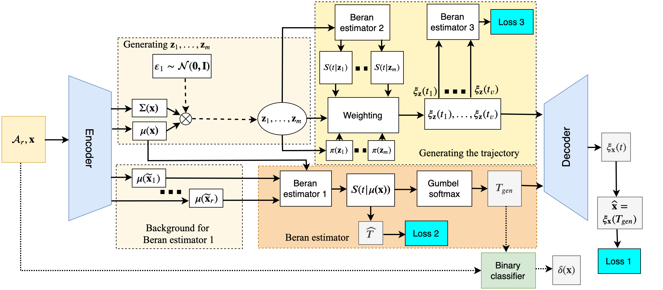
Figure 1: A scheme of the proposed model

3.1 Encoder part and training epochs

The first part of the VAE is the encoder which provides parameters $\mu(\mathbf{x})$ and $\Sigma(\mathbf{x})$ for generating embeddings in the hidden space producing the time trajectory and parameters $\mu(\widetilde{\mathbf{x}})$ and $\Sigma(\widetilde{\mathbf{x}})$ for generating embeddings to “learning” the Beran estimator. The encoder converts input feature vectors $\mathbf{x}$ into the hidden space $Z$. According to the standard VAE, the mapping is performed using the “reparametrization trick”. Each training epoch includes solving $M$ tasks such that each task consists of the following set:

$$\{\underbrace{(\widetilde{\mathbf{x}}_{i},T_{i},\delta_{i}),i=1,...,r}_{\text{background in the Beran estimator}},\underbrace{\mathbf{x,}T,\delta}_{\text{input instance}}\}.$$ (8)

The training dataset in this case contains the following triplets: $(\widetilde{\mathbf{x}}_{i},T_{i},\delta_{i})$, $i=1,...,r$, which form the datasubset $\mathcal{A}_{r}\subset\mathcal{A}$, and the triplet $(\mathbf{x},T,\delta)$ which is taken from the dataset $\mathcal{A}\backslash\mathcal{A}_{r}$ during training and is a new instance during inference. Here $r$ is a hyperparameter. In order to differ the points from $\mathcal{A}_{r}$ and $\mathcal{A}\backslash\mathcal{A}_{r}$, we denote the selected feature vectors in $\mathcal{A}_{r}$ as $\widetilde{\mathbf{x}}$. Thus, $M$ sets $\mathcal{A}_{r}$ of $r$ points are selected on each epoch, which are used as the training set, and the remaining $n-r$ points are processed through the model directly and are passed to the loss function, after which the optimization is performed by the error backpropagation. After training the model on several epochs, the background for the Beran estimator is set to the entire training set.

In order to describe the whole scheme of training and using the VAE, we consider two subsets of vectors generated by the encoder. The first subset corresponding to the upper path in the scheme in Fig. 1 (Generating $\mathbf{z}_{1},,,.,\mathbf{z}_{m}$) consists of two vectors: $\mu(\mathbf{x})$ (mean values) and $\Sigma(\mathbf{x})$ (standard deviations). It should be noted that we consider $\Sigma$ as a vector, but not as a covariance matrix, because we aim to get uncorrelated features in the embedding space $\mathcal{Z}$ of the VAE. These parameter vectors are used to generate random vectors $\mathbf{z}_{1},,,.,\mathbf{z}_{m}$ calculated as $\mathbf{z}_{i}=\mu(\mathbf{x})+\varepsilon_{1}\cdot\Sigma(\mathbf{x})$, where $\varepsilon_{1}$ is the normally generated vector of noise $\varepsilon_{1}\sim\mathcal{N}(\mathbf{0},\mathbf{I})$, $\mathbf{0}=(0,...0)$, $\mathbf{I}=(1,...1)$. Vectors $\mathbf{z}_{1},,,.,\mathbf{z}_{m}$ are used for training as well as for inference. They are located around $\mu(\mathbf{x})$ and form a set $\mathcal{D}_{m}$ of normally distributed points, which is schematically shown in Fig. 2. The set $\mathcal{D}_{m}$ is used to compute the robust trajectory $\xi_{\mathbf{z}}(t)$.

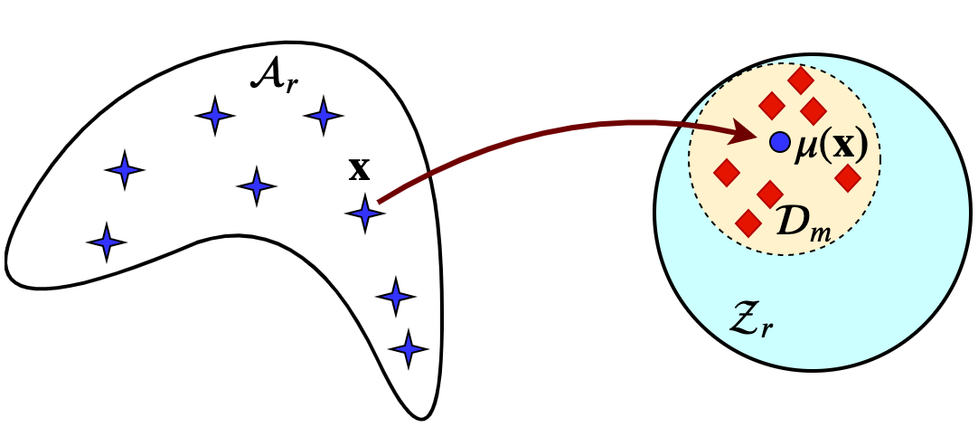
Figure 2: The original set $\mathcal{A}_{r}$ of vectors $\mathbf{x}_{i}$ and the set $\mathcal{D}_{m}$ of vectors $\widetilde{\mathbf{z}}_{1},...,\widetilde{\mathbf{z}}_{m}$ normally distributed around vector $\mathbf{z}$

The second subset of vectors generated by the encoder consists of the functions $\mu(\widetilde{\mathbf{x}}_{1}),...\mu(\widetilde{\mathbf{x}}_{r})$ of the vectors $\widetilde{\mathbf{x}}_{1},...,\widetilde{\mathbf{x}}_{r}$ from $\mathcal{A}_{r}$. In this case, the set $\mathcal{A}_{r}$ is selected from the entire dataset to learn the Beran estimator which is used to predict the SF and the expected event time for the vector $\mu(\mathbf{x})$. Therefore, vectors $\mu(\widetilde{\mathbf{x}}_{1}),...\mu(\widetilde{\mathbf{x}}_{r})$ can be regarded as the background for the Beran estimator. In contrast to vectors $\mathbf{z}_{1},,,.,\mathbf{z}_{m}$ which are generated for the feature vector $\mathbf{x}$, each vector $\mu(\widetilde{\mathbf{x}}_{i})$ is generated for the vector $\widetilde{\mathbf{x}}_{i}$ from $\mathcal{A}_{r}$. The second pair corresponds to the bottom path in the scheme in Fig. 1 (Background for Beran estimator 1).

3.2 The prototype embedding trajectory

Let us consider how to use the trained survival model (the Beran estimator) to compute the SF $S(t\mid\mathbf{z})$ and the trajectory $\xi_{\mathbf{z}}(t)$ (see Generating trajectory in Fig. 1).

Let $0<t_{1}<...<t_{n}$ be the distinct times to event of interest from the set $\{T_{1},...,T_{n}\}$, where $t_{1}=\min_{k=1,...,n}T_{k}$ and $t_{n}=\max_{k=1,...,n}T_{k}$. Suppose that a new vector $\mathbf{x}$ is fed to the encoder of the VAE. The encoder produces vectors $\mu(\mathbf{x})$ and $\Sigma(\mathbf{x})$. In accordance with these parameters and the random noise $\varepsilon_{1}$, the random embeddings $\mathbf{z}_{1},...,\mathbf{z}_{m}$ are generated from the normal distribution $\mathcal{N}(\mu(\mathbf{x}),\Sigma(\mathbf{x}))$. For every $\mathbf{z}_{i}$ from $\mathcal{D}_{m}$, we can find the density function $\pi(t\mid\mathbf{z}_{i})$ by using the trained survival model predicting the SF $S(t\mid\mathbf{z}_{i})$. The density function can be expressed through the SF $S(t\mid\mathbf{z}_{i})$ as:

$$\pi(t\mid\mathbf{z}_{i})=-\frac{\mathrm{d}S(t\mid\mathbf{z}_{i})}{\mathrm{d}t}.$$ (9)

However, our goal is to find another density function $\pi(\mathbf{z}_{i}\mid t)$ which allows us to generate the vectors $\mathbf{z}_{i}$ at different time moments. The density $\pi(\mathbf{z}_{i}\mid t)$ can be computed by using the Bayes rule:

$$\pi(\mathbf{z}_{i}\mid t)=\dfrac{\pi(t\mid\mathbf{z}_{i})\cdot\pi(\mathbf{z}_{i})}{\pi(t)}.$$ (10)

Here $\pi(\mathbf{z}_{i})$ is a priori density which can be estimated by applying several ways, for example, by means of the kernel density estimator. The density $\pi(t)$ can be estimated by using the Kaplan-Meier estimator. However, we do not need to estimate it because it can be regarded as a normalizing coefficient.

Now we have everything to compute $\pi(\mathbf{z}_{i}\mid t)$ and can consider how to use it to generate new points in accordance with this density.

Let us introduce a prototype embedding trajectory $\xi_{\mathbf{z}}(t)$ taking a value at each time $t$ as a mean value of vectors $\mathbf{z}_{i}$, $i=1,...,m$, with respect to densities $\pi(\mathbf{z}_{i}\mid t)$, $i=1,...,m$, as follows:

$$\xi_{\mathbf{z}}(t)=\sum_{i=1}^{m}\frac{\pi(\mathbf{z}_{i}\mid t)\cdot\mathbf{z}_{i}}{\sum_{j=1}^{m}\pi(\mathbf{z}_{j}\mid t)}.$$ (11)

After substituting the Bayes rule (10) into the expression for the trajectory (11), we obtain

$$\xi_{\mathbf{z}}(t)=\sum_{i=1}^{m}\frac{\pi(t\mid\mathbf{z}_{i})\cdot\pi(\mathbf{z}_{i})\cdot\mathbf{z}_{i}}{\sum_{j=1}^{m}\pi(t\mid\mathbf{z}_{j})\cdot\pi(\mathbf{z}_{j})}=\sum_{i=1}^{m}\alpha_{i}(t)\cdot\mathbf{z}_{i},$$ (12)

where $\alpha_{i}(t)$ is a normalized weight of each $\mathbf{z}_{i}$ in the trajectory at time $t$, which defined as

$$\alpha_{i}(t)=\frac{\pi(t\mid\mathbf{z}_{i})\cdot\pi(\mathbf{z}_{i})}{\sum_{j=1}^{m}\pi(t\mid\mathbf{z}_{j})\cdot\pi(\mathbf{z}_{j})}.$$ (13)

It can be seen from (12) that the trajectory $\xi_{\mathbf{z}}(t)$ is the weighted sum of generated vectors $\mathbf{z}_{i}$, $i=1,...,m$, depicted in Fig. 1 as the block “Weighting”. As a result, we obtain the robust trajectory for the latent representation $\mathbf{z}$ or $\mu(\mathbf{x})$.

Let us consider how to compute the density $\pi(t\mid\mathbf{z}_{i})$ in accordance with the Beran estimator (Beran estimator 2 in Fig. 1). First, the SF $S(t\mid\mathbf{z}_{i})$ is determined by using (5) as:

$$S(t\mid\mathbf{z}_{i})=\prod_{\widetilde{T}_{i}\leq t}\left\{1-\frac{W(\mathbf{z}_{i},\mu(\widetilde{\mathbf{x}}_{i}))}{1-\sum_{j=1}^{i-1}W(\mathbf{z}_{j},\mu(\widetilde{\mathbf{x}}_{j}))}\right\}^{\delta_{i}},$$ (14)

where $\widetilde{T}_{i}$ is the event time corresponding to the vector $\widetilde{\mathbf{x}}_{i}$ from $\mathcal{A}_{r}$.

Second, due to the final number of training instances, the Beran estimator provides a step-wise SF represented as follows:

$$S(t\mid\mathbf{z}_{i})=\sum\limits_{j=0}^{n-1}S_{j}\cdot\mathbb{I}\{t\in[t_{j},t_{j+1})\},$$ (15)

where $S_{j}=S(t_{j}\mid\mathbf{z}_{i})$ is the SF in the time interval $[t_{j},t_{j+1}]$ obtained from (5); $S_{0}=1$ by $t_{0}=0$; $\mathbb{I}\{t\in[t_{j},t_{j+1})\}$ is the indicator function taking the value $1$ if $t\in[t_{j},t_{j+1})$, and $0$, otherwise.

The probability density function $\pi(t\mid\mathbf{z}_{i})$ can be calculated as:

$$\pi(t|\mathbf{z}_{i})=\sum_{j=0}^{n-1}\left(S_{j}-S_{j+1}\right)\cdot\mathbb{\delta}\{t=t_{j}\},$$ (16)

where $\mathbb{\delta}\{t=t_{j}\}$ is the Dirac delta function.

Let us replace the density $\pi(t\mid\mathbf{z}_{i})$ with the discrete probability distribution $\left(p(t_{1}\mid\mathbf{z}_{i}),...,p(t_{n}\mid\mathbf{z}_{i})\right)$ such that $p(t_{j}\mid\mathbf{z}_{i})=S_{j-1}-S_{j}$. Then (13) can be represented in another form:

$$\alpha_{i}(t_{j})=\frac{p(t_{j}\mid\mathbf{z}_{i})\pi(\mathbf{z}_{i})}{\sum_{l=1}^{m}p(t_{j}\mid\mathbf{z}_{l})\cdot\pi(\mathbf{z}_{l})},\ j=1,...,n.$$ (17)

Since coefficients $\alpha_{1},...,\alpha_{m}$ are normalized, then they form the convex combination of $\mathbf{z}_{1},...,\mathbf{z}_{m}$.

Vectors $\mathbf{z}_{i}$ are governed by the normal distribution $\mathcal{N}(\mu(\mathbf{x}),\Sigma(\mathbf{x}))$, therefore, the density $\pi(\mathbf{z}_{i})$ is determined as

$$\pi(\mathbf{z}_{i})\varpropto\exp\left(-\frac{1}{2}(\mathbf{z}_{i}-\mu(\mathbf{x}))^{\top}\left(\Sigma(\mathbf{x})\right)^{-1}(\mathbf{z}_{i}-\mu(\mathbf{x}))\right).$$ (18)

It is important to point out that $p(t\mid\mathbf{z}_{i})$ as well as $\pi(t\mid\mathbf{z}_{i})$ are defined at time points $t_{1},...,t_{n}$. However, when the trajectory is constructed, it is necessary to ensure that the model takes into account the entire context. To cope with this difficulty, we propose to smooth the density function $\pi(t\mid\mathbf{z}_{i})$ to obtain a smooth trajectory. The smoothing is carried out using a convex combination with coefficients $\{\beta_{1}(t),...,\beta_{n}(t)\}$ determined by means of the softmin operation with respect to the distance from $t$ to $\{t_{1},...,t_{n}\}$, respectively. Then we can write for the smooth version of $\pi(t\mid\mathbf{z}_{i})$ denoted as $\widetilde{\pi}(t\mid\mathbf{z}_{i})$:

$$\widetilde{\pi}(t\mid\mathbf{z}_{i})=\sum\limits_{i=1}^{n}\beta_{i}(t)\cdot\pi(t_{i}\mid\mathbf{z}_{i}),$$ (19)

where

$$\beta_{i}(t)=\mathrm{softmin}(\eta\cdot|t-t_{i}|),\ i=1,...,n,$$ (20)

$\eta$ is a training parameter; $\mathrm{softmin}(x)=\mathrm{softmax}(-x)$.

The trajectory $\xi_{\mathbf{z}}(t)$ is determined for the finite set of time moments $t_{1},...,t_{v}$ which are selected as follows: $t_{k}=t_{k-1}+(t_{\max}-t_{\min})/v$, where $t_{\min}$, $t_{\max}$ are the smallest and the largest times to event from the training set, $t_{0}=t_{\min}$, $k=1,...,v$.

In order to compute the corresponding prototype trajectory $\xi_{\mathbf{x}}(t)$ for the vector $\mathbf{x}$, we use the decoder of the VAE. The prototype trajectory $\xi_{\mathbf{x}}(t)$ at each time moment can be viewed as some points in the dataset domain, i.e., for each time $t_{j}$, we can construct a point (vector) $\xi_{\mathbf{x}}(t_{j})\in\mathbb{R}^{d}$ at the trajectory $\xi_{\mathbf{x}}(t)$ . The trajectory means which features should be changed in $\mathbf{x}$ to achieve a certain time $t$ to event.

3.3 New data generation and the censored indicator

Another task which can be solved in the framework of the proposed model is to generate a new survival instance in accordance with the available dataset $\mathcal{A}$. First, we train the Beran estimator (Beran estimator 1 in Fig. 1) on the set of vectors $\mu(\widetilde{\mathbf{x}}_{1}),...\mu(\widetilde{\mathbf{x}}_{r})$. For the vector $\mu(\mathbf{x})$ corresponding to the input vector $\mathbf{x}$, the SF $S(t\mid\mu(\mathbf{x}))$ can be estimated by using Beran estimator 1 as follows:

$$S(t\mid\mu(\mathbf{x}))=\prod_{\widetilde{T}_{i}\leq t}\left\{1-\frac{W(\mu(\mathbf{x}),\mu(\widetilde{\mathbf{x}}_{i}))}{1-\sum_{j=1}^{i-1}W(\mu(\mathbf{x}),\mu(\widetilde{\mathbf{x}}_{j}))}\right\}^{\delta_{i}}.$$ (21)

Here $\widetilde{T}_{i}$ is the event time corresponding to the vector $\widetilde{\mathbf{x}}_{i}$ from $\mathcal{A}_{r}$. Hence, a new time $T_{gen}$ is generated in accordance with $S(t\mid\mu(\mathbf{x}))$ by applying the Gumbel sampling which has already been used in autoencoders [25].

By having the reconstructed trajectory $\xi_{\mathbf{x}}(t)$ and the time $T_{gen}$, we generate a feature vector $\widehat{\mathbf{x}}=\xi_{\mathbf{x}}(T_{gen})$ and write a new instance $(\widehat{\mathbf{x}},T_{gen})$. However, a complete description of the instance requires to determine the censored indicator $\delta_{gen}$. In order to find $\delta_{gen}$ for $(\widehat{\mathbf{x}},T_{gen})$, we introduce a binary classifier which considers each pair $(\mathbf{x}_{i},T_{i})$ from the training set as a single feature vector, but $\delta_{i}$ from the training set as a class label taking values $0$ (a censored event) and $1$ (an uncensored event). If the binary classifier is trained on the training set $((\mathbf{x}_{i},T_{i}),\delta_{i})$, $i=1,...,n$, then $\delta_{gen}$ can be predicted on the basis of the feature vector $(\widehat{\mathbf{x}},T_{gen})$. Finally, we obtain the triplet $(\widehat{\mathbf{x}},T_{gen},\delta_{gen})$. If the classifier predicts probabilities of two classes, then the Bernoulli distribution is applied to generate $\delta_{gen}$. It is important to note that the binary classifier is trained separately from the VAE training.

It should be noted that the SF $S(t\mid\mu(\mathbf{x}))$ in (15) is also used for computing the expected time $\widehat{T}$ to event which is of the form:

$$\widehat{T}=\sum\limits_{i=0}^{n-1}S_{i}\cdot(t_{i+1}-t_{i}).$$ (22)

The expected time is required for its use in the loss function $\mathcal{L}_{\text{Beran}}$ (“Loss 2” in Fig. 1), which is considered below.

3.4 Decoder part

The decoder converts the trajectory $\xi_{\mathbf{z}}(t)$ into the trajectory $\xi_{\mathbf{x}}(t)$. It also produces the vector $\widehat{\mathbf{x}}$ which is used in the loss function $\mathcal{L}_{\text{WAE}}$. The loss function is schematically depicted in Fig. 1 as “Loss 1”.

3.5 Training the VAE

The entire model is trained in the end-to-end manner, excluding the part that generates the censored indicator $\delta_{gen}$. The loss function $\mathcal{L}$ consists of three parts: the first is responsible for the accurate estimation of the event times and denoted as $\mathcal{L}_{\text{Beran}}$, the second is responsible for the accurate reconstruction and denoted as $\mathcal{L}_{\text{WAE}}$, the third is for accurate estimation of the trajectory $\xi_{\mathbf{z}}(t)$ at time moments $t_{1},...,t_{v}$ denoted as $\mathcal{L}_{\text{Tr}}$. Hence, there holds

$$\mathcal{L}=-\mathcal{L}_{\text{Beran}}+\mathcal{L}_{\text{WAE}}-\mathcal{L}_{\text{Tr}}.$$ (23)

Below $\gamma_{1}$, $\gamma_{2}$, $\gamma_{3}$, and $\gamma_{4}$ are hyperparameters controlling contributions of the corresponding parts of the loss function.

The loss function $\mathcal{L}_{\text{Beran}}$ (depicted as “Loss 2” in Fig. 1) is based on the use of the C-index softened with a sigmoid function $\sigma$:

$$\mathcal{L}_{\text{Beran}}=\gamma_{1}\frac{\sum_{i,j}\mathbb{I}\{t_{j}<t_{i}\}\cdot\sigma(\hat{T}_{i}-\hat{T}_{j})\cdot\delta_{j}}{\sum_{i,j}\mathbb{I}\{t_{j}<t_{i}\}\cdot\delta_{j}}.$$ (24)

It is included in $\mathcal{L}$ with minus because $\mathcal{L}_{\text{Beran}}$ should be maximized. The temperature parameter $\tau$ of the kernel (7) in the Beran estimator is also trained due to $\mathcal{L}_{\text{Beran}}$.

The loss function $\mathcal{L}_{\text{WAE}}$ (“Loss 1” in Fig. 1) consists of the mean squared error on reconstructions and of the regularization $\mathcal{L}_{\text{MMD}}$ in the form of the maximum mean discrepancy [24]:

$$\mathcal{L}_{\text{WAE}}=\frac{\gamma_{2}}{n}\sum\limits_{i=1}^{n}\left\|\mathbf{x}_{i}-\widehat{\mathbf{x}}_{i}\right\|^{2}+\mathcal{L}_{\text{MMD}},$$ (25)

where $\widehat{\mathbf{x}}_{1},...,\widehat{\mathbf{x}}_{n}$ are conditionally generated according to the formula $\widehat{\mathbf{x}}=\xi_{\mathbf{x}}(T_{gen})$.

Note that the sets of embeddings $\{\mathbf{z}_{1}^{(i)},,,.,\mathbf{z}_{m}^{(i)}\}$ governed by the the normal distribution $\mathcal{N}(\mu(\mathbf{x}_{i}),\Sigma(\mathbf{x}_{i}))$ are generated $n$ times for every $\mathbf{x}_{i}$, $i=1,...,n$. During training, we take the first embeddings $\mathbf{z}_{1}^{(i)}$ for all $i=1,...,n$, and compare them with the embeddings $\widehat{\mathbf{z}}_{i}$ sampled from the normal distribution $\mathcal{N}(\mathbf{0},\mathbf{1})$. To ensure that all embeddings, including $\mu(\mathbf{x}_{i})$, are normally distributed, the following regularization is used:

$$\mathcal{L}_{\text{MMD}} =\frac{\lambda}{n(n-1)}\sum\limits_{l,j=1,l\neq j}^{n}K(\mathbf{z}_{l},\mathbf{z}_{j})+\frac{\lambda}{n(n-1)}\sum\limits_{l,j=1,l\neq j}^{n}K(\widehat{\mathbf{z}}_{i},\widehat{\mathbf{z}}_{j})$$

$$-\frac{2\lambda}{n^{2}}\sum\limits_{l=1}^{n}\sum\limits_{j=1}^{n}K(\mathbf{z}_{l},\widehat{\mathbf{z}}_{j}),$$ (26)

where $K(\mathbf{x},\mathbf{y})=C/(C+||\mathbf{x}-\mathbf{y}||_{2}^{2})$ is a positive-define kernel with the parameter $C=2\cdot\dim(\mathbf{z}{)}$; $\lambda\geq 0$ is a hyperparameter.

The loss function $\mathcal{L}_{\text{Tr}}$ (“Loss 3” in Fig. 1) consists of two parts $\mathcal{L}_{\text{Tr1}}$ and $\mathcal{L}_{\text{Tr2}}$. The loss function $\mathcal{L}_{\text{Tr1}}$ is similar to $\mathcal{L}_{\text{Beran}}$, but it controls how the expected event times $\hat{T}_{1},...,\hat{T}_{v}$ obtained for elements of the trajectory $\xi_{\mathbf{z}}(t_{1}),...,\xi_{\mathbf{z}}(t_{v})$ by means of the Beran estimator 3 are consistent with the corresponding event times $t_{1},...,t_{v}$:

$$\mathcal{L}_{\text{Tr1}}=\gamma_{3}\frac{\sum_{i,j}\mathbb{I}\{t_{j}<t_{i}\}\cdot\sigma(\hat{T}_{i}-\hat{T}_{j})\cdot\delta_{j}}{\sum_{i,j}\mathbb{I}\{t_{j}<t_{i}\}\cdot\delta_{j}}.$$ (27)

The second term $\mathcal{L}_{\text{Tr2}}$ of the loss function $\mathcal{L}_{\text{Tr}}$ can be regarded as a regularization for the densities ${\pi(T_{i}|\xi_{\mathbf{z}_{i}}(T_{i}))}$ by using the Beran estimator 3 and allows us to obtain more elongated trajectories. This can be implemented by using the likelihood function:

$$\mathcal{L}_{\text{Tr2}}=\gamma_{4}\sum\limits_{i=1}^{n_{u}}\alpha_{i}\log{\pi(T_{i}|\xi_{\mathbf{z}_{i}}(T_{i})).}$$ (28)

Here ${T_{i}}$ are the event times from the training set; $n_{u}$ is the number of uncensored instances in the training set (only uncensored instances are used in $\mathcal{L}_{\text{Tr2}}$); ${\xi_{\mathbf{z_{i}}}}$ is the trajectory for the embedding $\mathbf{x}_{i}$; ${\pi}$ is the density function computed by using the Beran estimator; $\alpha_{i}$ are smoothing weights computed as:

$$\alpha_{i}=\text{softmin}(\{\pi_{K-M}(T_{1}),\pi_{K-M}(T_{2}),...,\pi_{K-M}(T_{n_{u}})\})_{i},$$ (29)

where $\pi_{K-M}(t)$ is the probability density of the event time obtained by using the Kaplan-Meier estimator over the entire dataset.

Each training epoch includes solving $M$ tasks such that each task consists of a set of data (8).

The training dataset in this case consists of the following triplets: $(\mathbf{x}_{i},T_{i},\delta_{i})$, $i=1,...,n$. Thus, $M$ sets of $r+1$ points are selected on each epoch, which are used as the training set, and the remaining $n-r-1$ points are processed through the model directly and are passed to the loss function, after which the optimization is performed by the error backpropagation. After training the model on several epochs, the background for the Beran estimator is set to the entire training set.

4 Numerical experiments

Numerical experiments are performed in the following three directions:

1. Experiments with synthetic data.

2. Experiments with real data, which illustrate the generation of synthetic points in accordance with the real dataset.

3. Experiments with real data for constructing the survival regression models.

4.1 Experiments with synthetic data

In all experiments, we study the proposed model using instances with two clusters. The cluster structure of data is used to complicate conditions of the generation. Instances have two features, i.e., $\mathbf{x}\in\mathbb{R}^{2}$. They are represented on the graphs in 3D, time is located along the $Oz$ axis ($\hat{T}$ or $T_{gen}$, to be specified separately). We perform the unconditional generation. The number of sampled points in experiments is the same as the number of points in the training dataset. When performing the conditional generation, we consider both the time generated using the Gumbel softmax operation and the expected event time.

The following parameters of numerical experiments for synthetic data are used: the length of embeddings $\mathbf{z}_{i}$ is $8$; the number of embeddings $\mathbf{z}_{i}$ in the weighting scheme is $m=48$;

Hyperparameters of the loss function (23): parameter $\lambda$ in (26) is $40$; $\gamma_{1}=0.5$; $\gamma_{2}=2$; $\gamma_{3}=1$; $\gamma_{4}=0.05$;

4.1.1 “Linear” dataset

First, we study the linear synthetic dataset which is conditionally called “linear” because two clusters of feature vectors are located along straight lines and the event times are uniformly distributed over each cluster. Clusters are formed by means of four clouds of normally distributed points. Each point within a cluster is a convex combination of centers of clouds corresponding to the cluster adding the normal noise. Coefficients in the convex combination are generated with respect to the uniform distribution. The obtained clusters are depicted in Fig. 3 in red and blue colors. Fig. 3 illustrates how points $\widehat{\mathbf{x}}$ depicted by purple triangles are generated for input points $\mathbf{x}$ depicted by stars.

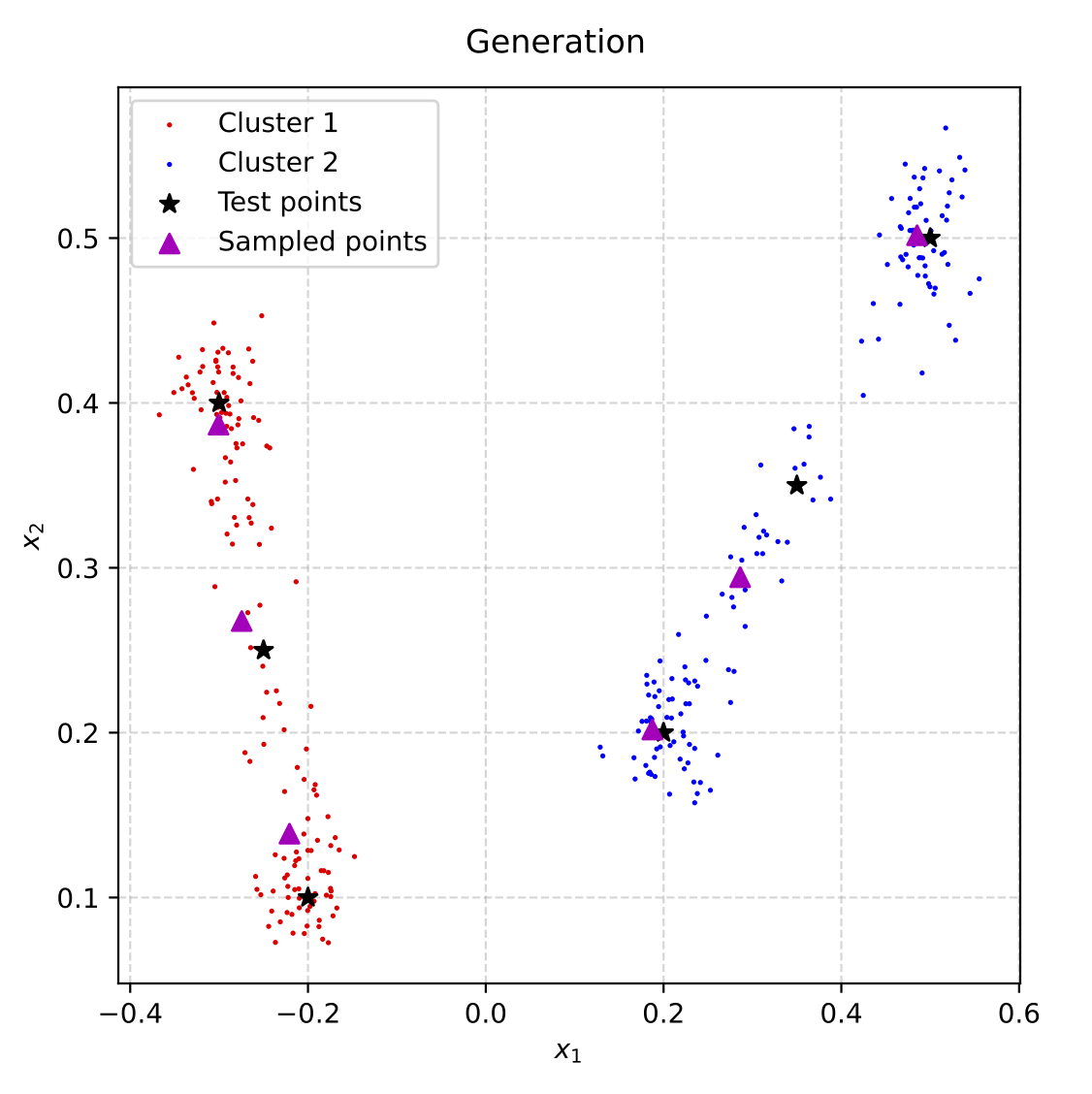
Figure 3: Illustration of generated points $\widehat{\mathbf{x}}$ for the “linear” dataset

Fig. 4 illustrates the same generation of points $\widehat{\mathbf{x}}$ depicted by black markers jointly with generated times to event $T_{gen}$. One can see from Fig. 4 that most points are close to the dataset points from the corresponding clusters. However, there are a few points located between clusters, which are generated incorrectly. Figs. 3 and 4 show that the proposed model mainly correctly reconstructs feature vectors and correctly generates the event times.

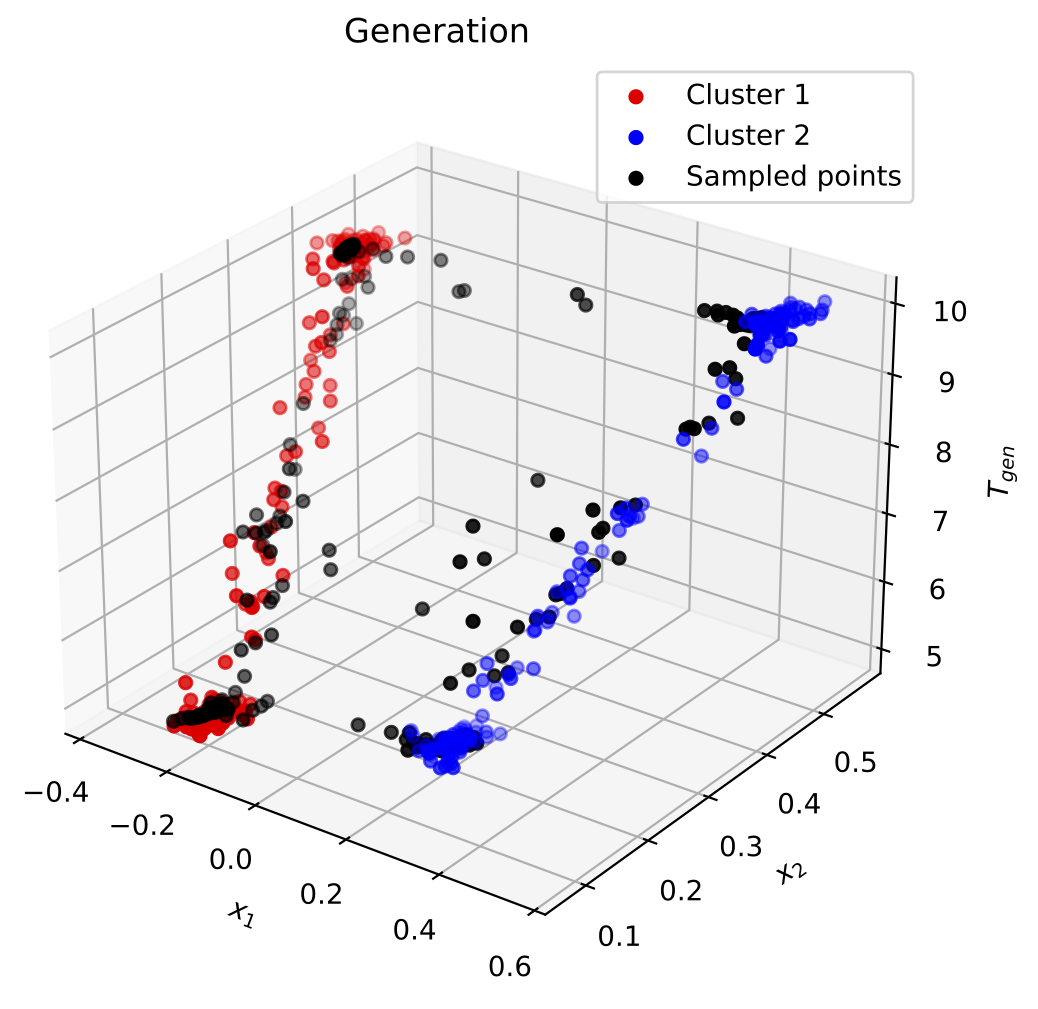
Figure 4: Generated points $(\widehat{\mathbf{x}},T_{gen})$ for the “linear” dataset

Generated trajectories for points A and B from the first and the second clusters, respectively, of the “linear” dataset are illustrated in Fig. 5 where the left picture shows only the generated points $\xi_{\mathbf{x}}$ without time moments, the right picture shows points of the same trajectory taking into account time moments $t_{1},...,t_{v}$. It can be seen from Fig. 5 that the generated trajectory corresponds to the location of points from the dataset. An example of the generated feature trajectories as functions of the time for the “linear” dataset also shown in Fig. 6. The point A is taken to generate the trajectory. It is important to note that the trajectories of each feature are rather smooth. This is due to the weighting procedure which is used to generate $\xi_{\mathbf{z}}(t)$ in the embedding space and due to the correct reconstruction of points by the VAE.

Figure 5: Generated trajectories for the “linear” dataset

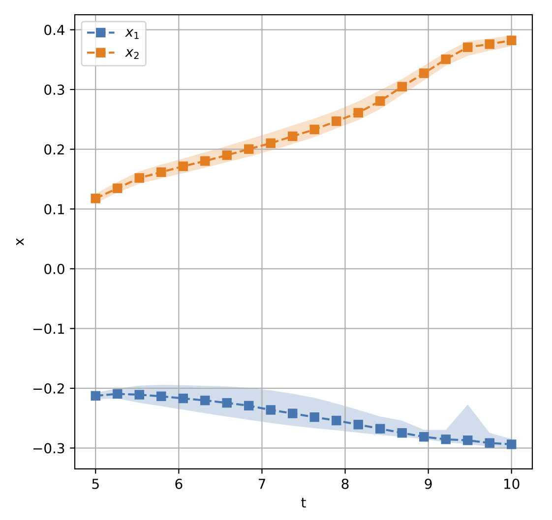
Figure 6: Generated trajectories of each feature as functions of the time for the “linear” dataset

4.1.2 Two parabolas

Let us consider an illustrative example with a dataset which is similar to the well-known “two moons” dataset, which can be found in the Python Scikit-learn package. In contrast to the use of the original “two moons” dataset, we complicate the task by considering two different clusters (parabolas) of data, but with similar event times. The event times are generated linearly from the feature $x_{1}$, so the values on each branch of each parabola are symmetrically located.

Results of generation of $T_{gen}$ and $\widehat{T}$ are depicted in the left and the right pictures of Fig. 7. One can see from Fig. 7 that points are mainly correctly generated. Moreover, the expected event time $\widehat{T}$ has smaller fluctuations than the generated one $T_{gen}$. This fact demonstrates that the model properly generates.

Figure 7: Generation of $T_{gen}$ and $\widehat{T}$ for the “two parabolas” dataset

Fig. 8 illustrates how trajectories for points A and B are generated. The left and the right pictures in Fig. 8 show the trajectories without the event times and with the times. It is explicitly seen that trajectories are generated on branches of the parabolas.

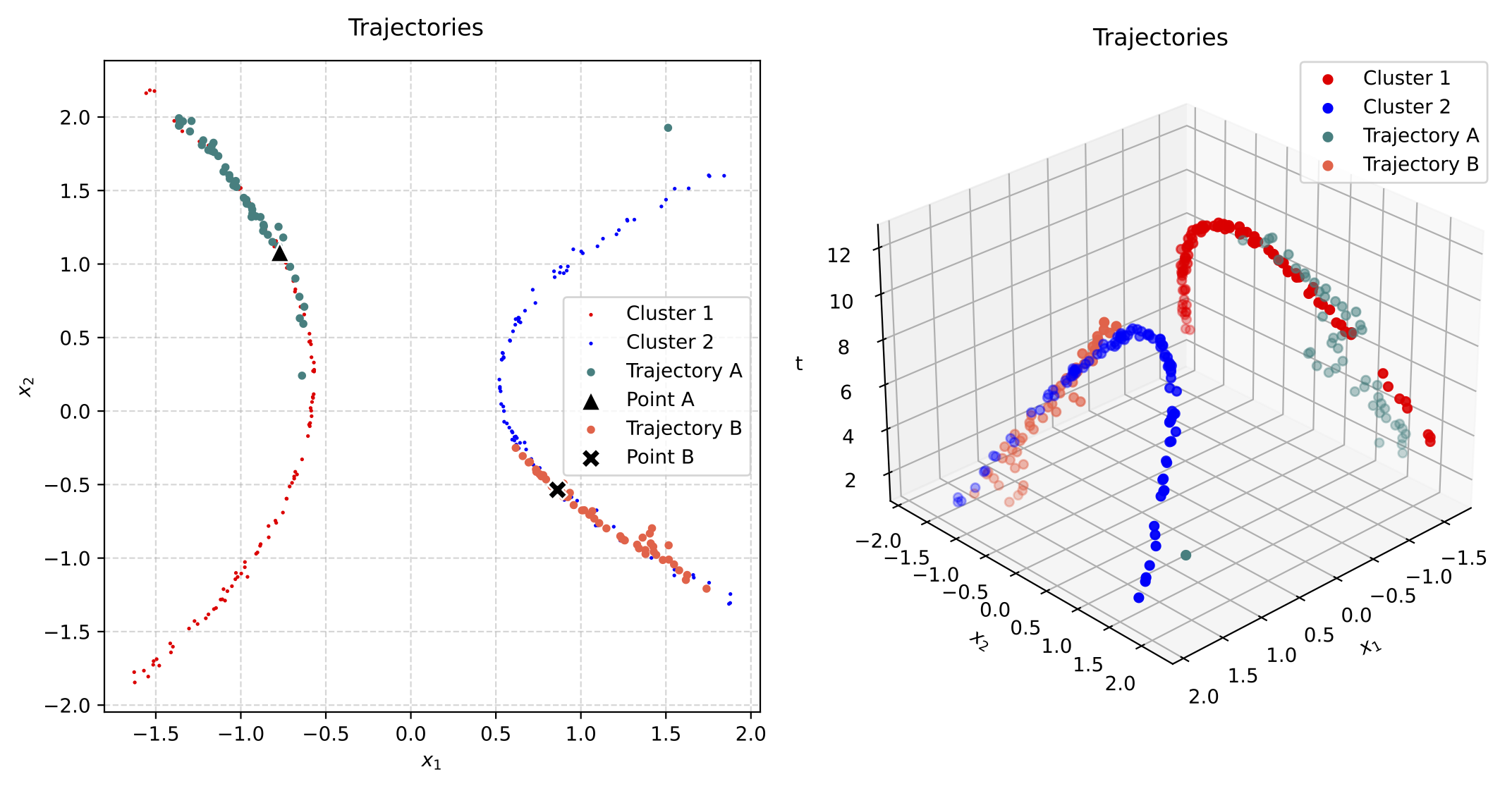
Figure 8: Generation of trajectories for points A and B by using the “two parabolas” dataset

Generated feature trajectories as functions of the time for the “two parabolas” dataset are shown in Fig. 9. The point A is taken to generate the trajectory.

Figure 9: Generated trajectories of each feature as functions of the time for the “two parabolas” dataset

4.1.3 Two circles

Another interesting synthetic dataset consists of two circles as it is shown in Fig. 10. More precisely, we are conducting the experiment not with full-fledged circles, but with their sectors. The essence of the experiment is that there are regions where the event time seriously differs for very close feature vectors. At the same time, the event times for points belonging to each circle are slightly differ. They are generated with a small noise.

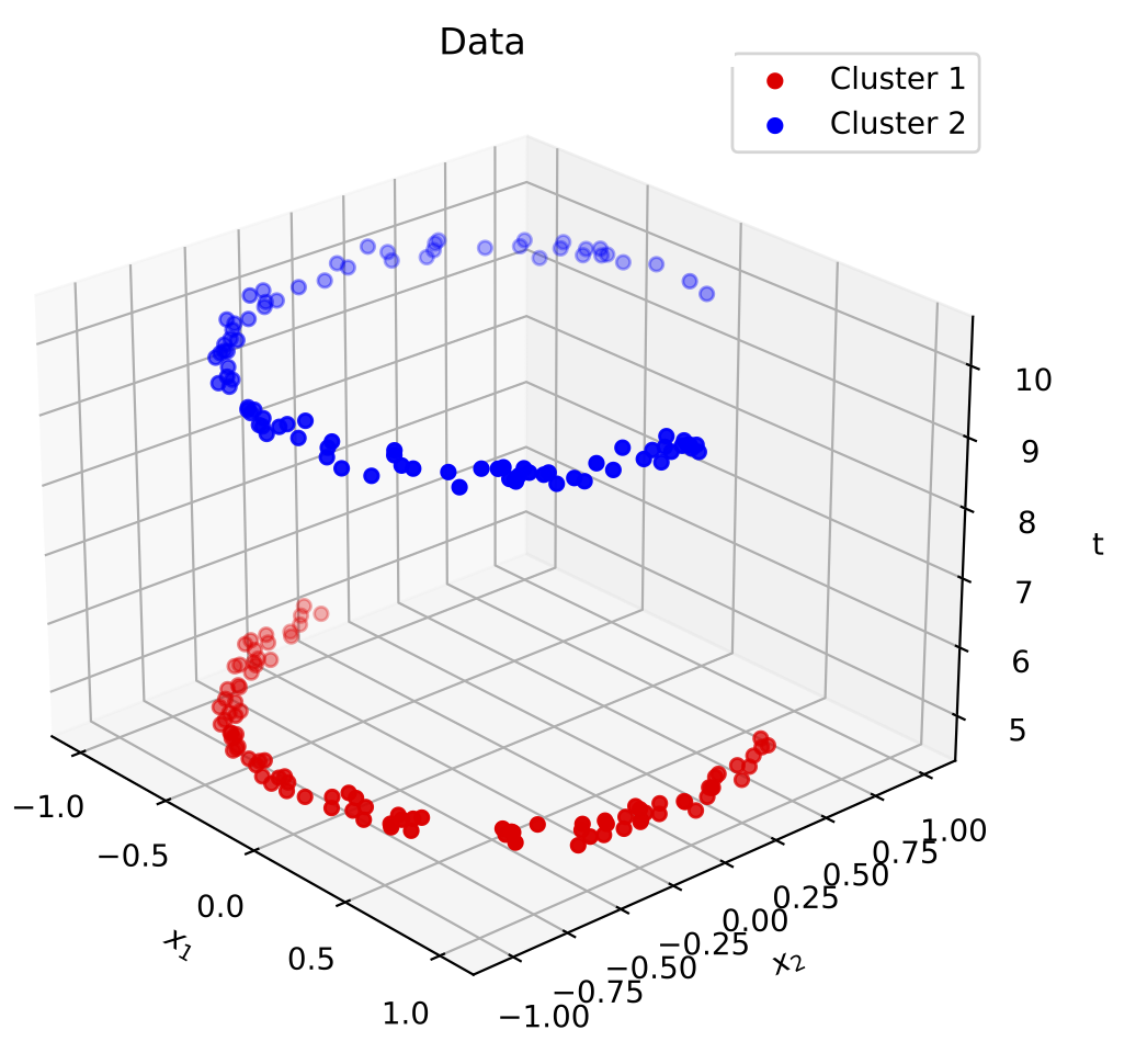
Figure 10: The “two circles” dataset

The left and the right pictures in Fig. 11 show results of generation of the event times $T_{gen}$ and the expected times $\widehat{T}$. It can be seen from Fig. 11 that the the event times $T_{gen}$ are correctly generated. This is due to the use of the Gumbel softmax operation. However, it follows from the right picture in Fig. 11 that the expected times give a strong bias which is caused by the multimodality of the probability distribution of the variables.

The task of the trajectory generation is not studied here because trajectories are simply be vertical in the 3D pictures in the overlapped area.

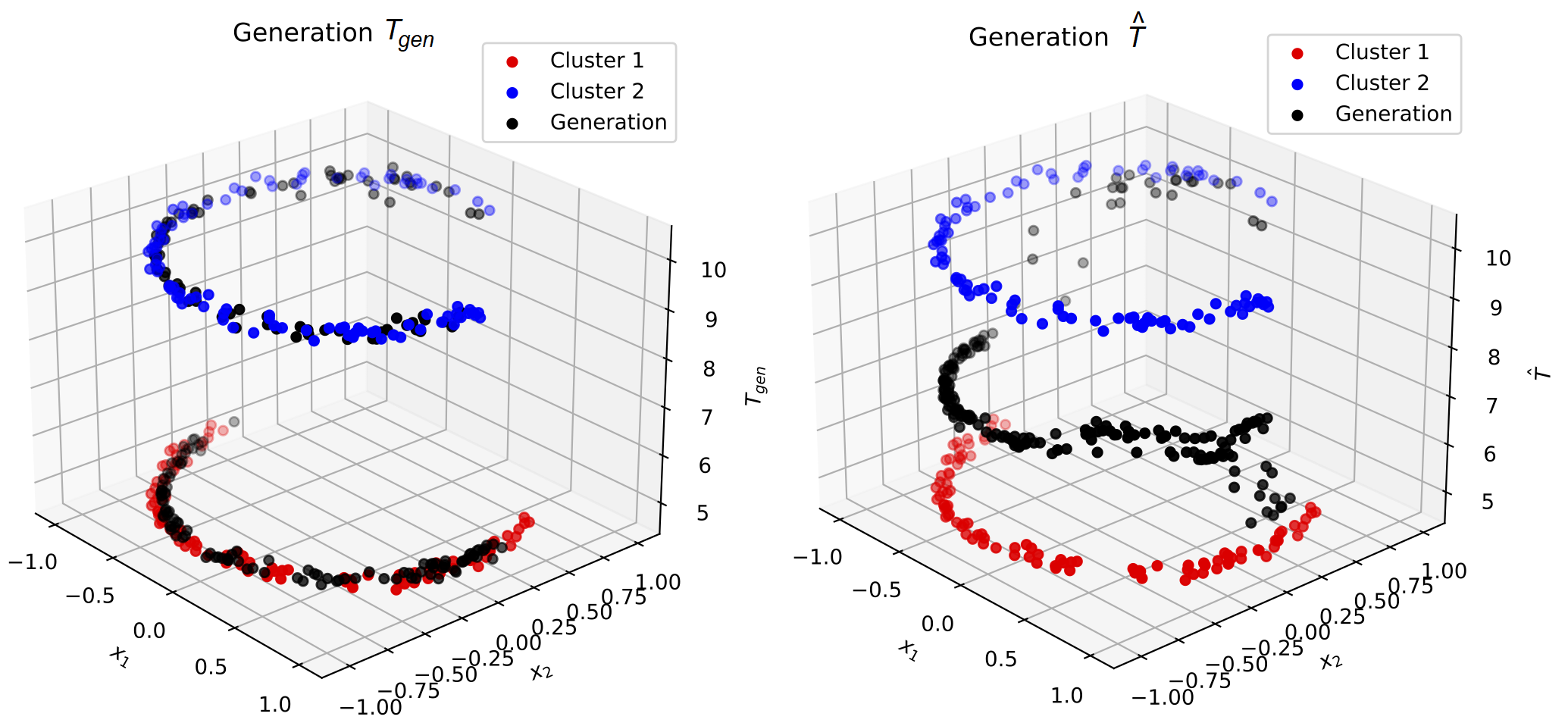
Figure 11: Generation of $T_{gen}$ and $\widehat{T}$ for the “two circles” dataset

4.2 Experiments with real data

The well-known real datasets, including the Veteran dataset, the WHAS500 dataset, and the GBSG2 dataset, are used for numerical experiments.

4.2.1 Veteran dataset

The first dataset is the Veterans’ Administration Lung Cancer Study (Veteran) Dataset [26] which contains data on 137 males with advanced inoperable lung cancer. The subjects were randomly assigned to either a standard chemotherapy treatment or a test chemotherapy treatment. The dataset can be obtained via the “survival” R package or the Python “scikit-survival” package.

By training and using the proposed model, we generate new instances in accordance with the Veteran dataset. Results are depicted in Fig. 12 where original points and the reconstructed points are shown in blue and red colors, respectively. The t-SNE method [27] is used to depict points in the 2D plot. It can be seen from Fig. 12 that the generated points support the complex cluster structure of the dataset. In order to study how the generated instances are close to the original data, we compute SFs for these two sets of instances by using the Kaplan-Meier estimator. The SFs are shown in Fig. 13. It can be seen from Fig. 13 that the SFs are very close to each other. This implies that the model provides a proper generation.

In order to depict the generated trajectory, we show how separate features should be changed to achieve a certain event time. The corresponding trajectories of the continuous features are depicted in Fig. 14. It is obvious that the feature “Age in years” cannot be changed in real life. However, our aim is to show that the trajectory is correctly generated. We can see that the age should be decreased to increase the event time. This indicates that the model correctly generates the trajectory.

Figure 12: Original and generated instances for the Veteran dataset

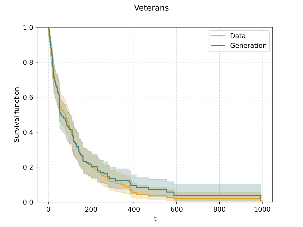
Figure 13: SFs constructed by means of the Kaplan-Meier estimator for original and generated data for the Veteran dataset

Figure 14: Trajectories of the continuous features generated for the Veteran dataset

4.2.2 WHAS500 dataset

Another dataset is the Worcester Heart Attack Study (WHAS500) Dataset [1]. It contains data on 500 patients having 14 features. The endpoint is death, which occurred for 215 patients (43.0%). The dataset can be obtained via the “smoothHR” R package or the Python “scikit-survival” package.

Similar results of experiments are shown in Figs. 15-17. In particular, original and generated points are depicted in Fig. 15 by using the t-SNE method in blue and red colors, respectively. SFs for original and generated points by using the Kaplan-Meier estimator are shown in Fig. 16. Trajectories of the continuous features are depicted in Fig. 17.

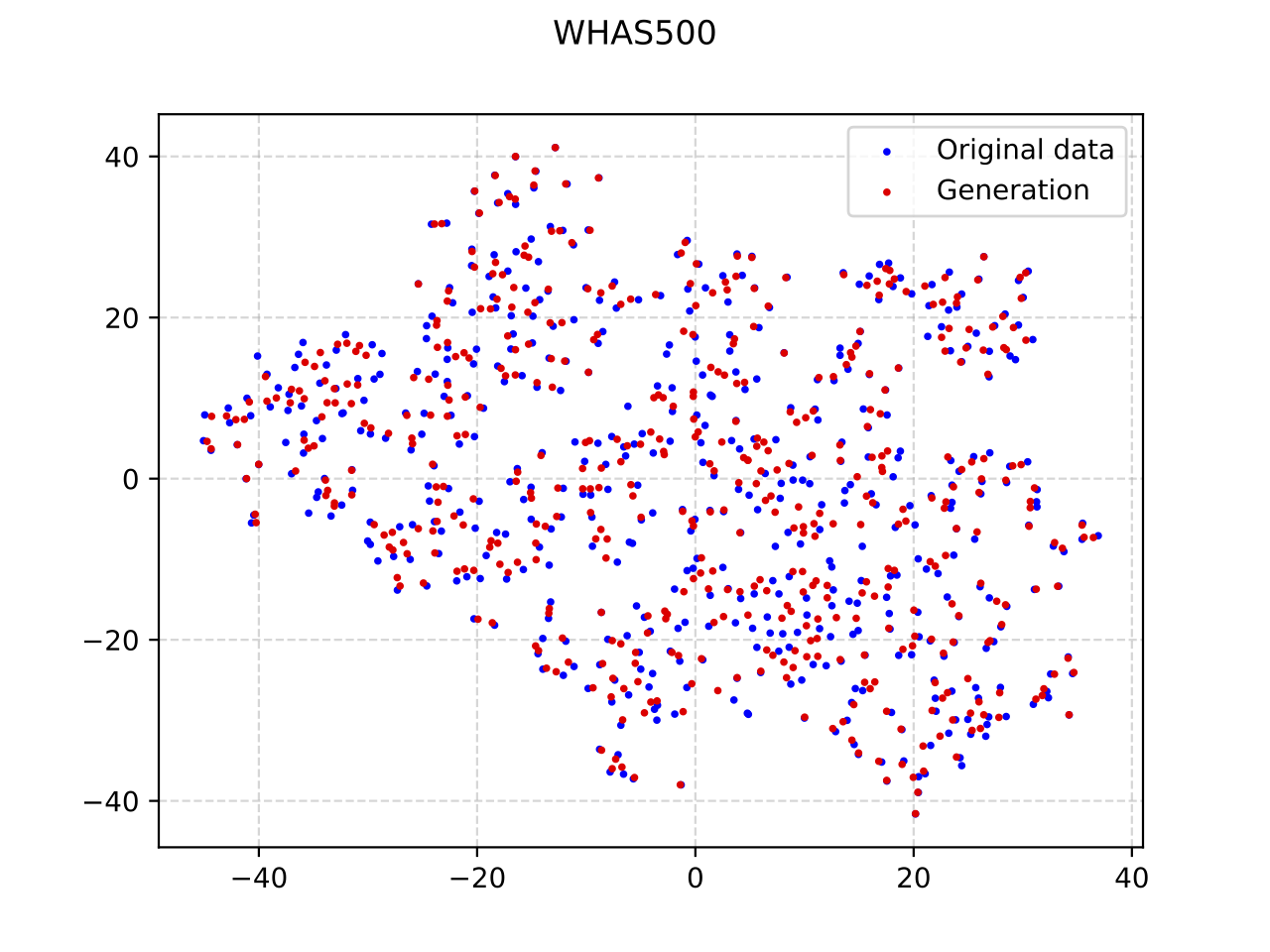
Figure 15: Original and generated instances for the WHAS500 dataset

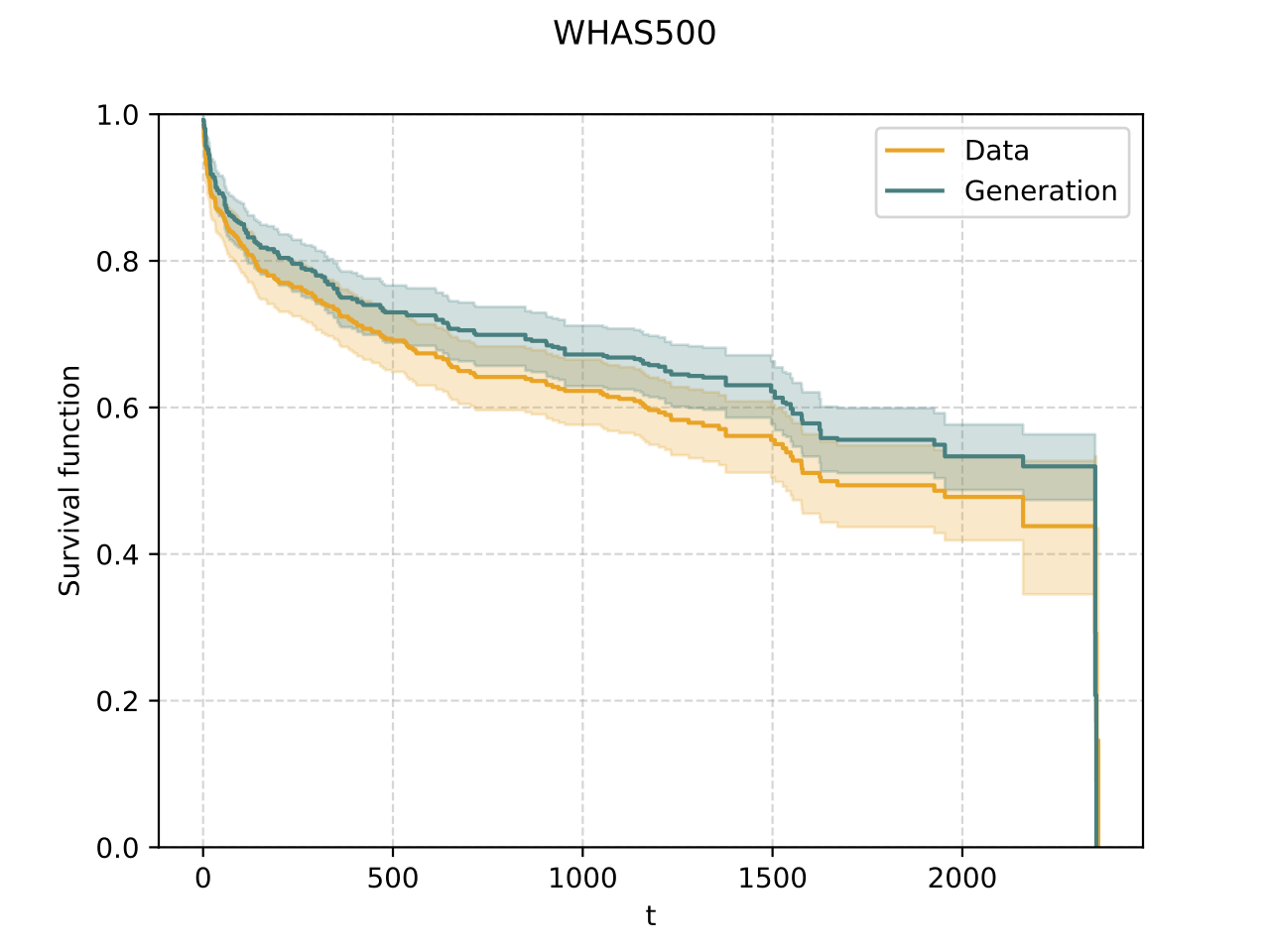
Figure 16: SFs constructed by means of the Kaplan-Meier estimator for original and generated data for the WHAS500 dataset

Figure 17: Trajectories of the continuous features generated for the WHAS500 dataset

4.2.3 GBSG2 dataset

The next dataset is the German Breast Cancer Study Group 2 (GBSG2) Dataset [28] which contains observations of 686 women. Every instance is characterized by 10 features, including age of the patients in years, menopausal status, tumor size, tumor grade, number of positive nodes, hormonal therapy, progesterone receptor, estrogen receptor, recurrence free survival time, censoring indicator (0 - censored, 1 - event). The dataset can be obtained via the “TH.data” R package or the Python “scikit-survival” package.

The original and generated points are depicted in Fig. 18 by using the t-SNE method in blue and red colors, respectively. SFs for original and generated points by using the Kaplan-Meier estimator are shown in Fig. 19. Trajectories of the continuous features are depicted in Fig. 20. In contrast to the previous datasets, where categorical features do not change in the defined time intervals, the categorical features of the GBSG2 dataset are changed. This change can be seen from Fig. 21. It is interesting to note that all trajectories have a jump at the same time $1940$. It is likely related to the unstable behavior of the model with respect to categorical features. Moreover, it is also interesting to note that changing one feature leads to changes in all features, indicating strong correlation between features of the considered dataset.

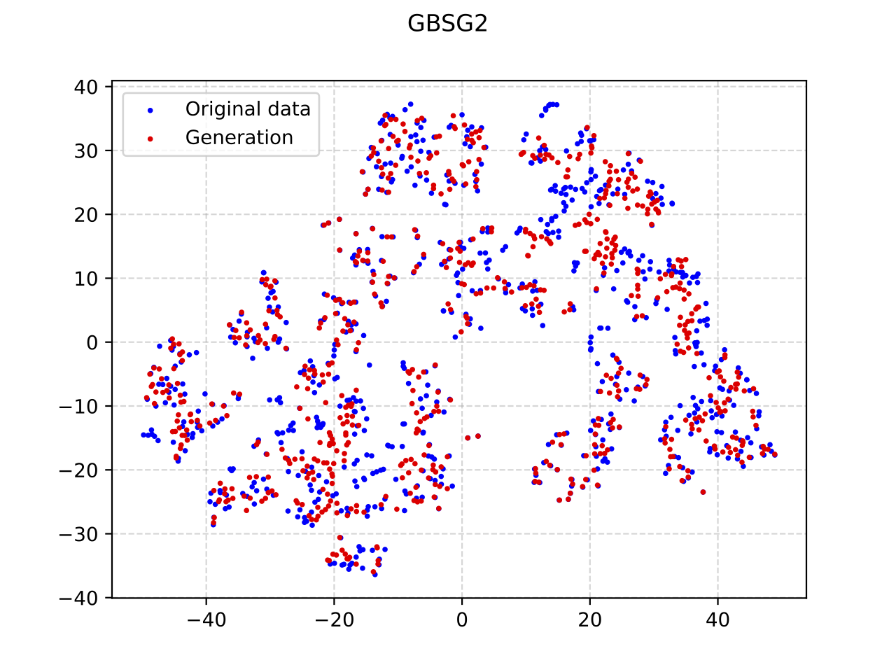
Figure 18: Original and generated instances for the GBSG2 dataset

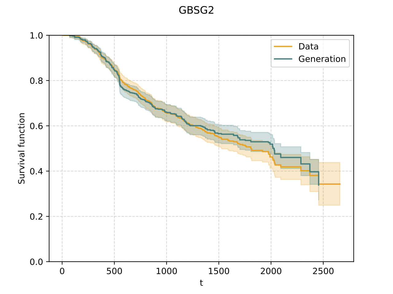
Figure 19: SFs constructed by means of the Kaplan-Meier estimator for original and generated data for the GBSG2 dataset

Figure 20: Trajectories of the continuous features generated for the GBSG2 dataset

Figure 21: Trajectories of the categorical features generated for the GBSG2 dataset

4.2.4 Prediction results

It has been mentioned that the proposed model provides accurate predictions. In order to compare the model with the Beran estimator [23], the Random Survival Forest [29], and the Cox-Nnet [30], we use the C-index. The corresponding results are shown in Table 1. To evaluate the C-index, we perform a cross-validation with $100$ repetitions, where in each run, we randomly select 75% of data for training and 25% for testing. Different values for hyperparameters models have been tested, choosing those leading to the best results. Hyperparameters of the Random Survival Forest used in experiments are the following: numbers of trees are $10$, $50$, $100$, $200$; depths are $3$, $4$, $5$, $6$; the smallest values of instances which fall in a leaf are one instance, 1%, 5%, 10% of the training instances. Values $10^{i}$, $i=-3,...,3$, and also values $0.5$, $5$, $50$, $200$, $500$, $700$ of the bandwidth parameter $\tau$ in the Gaussian kernel are selected as possible values of hyperparameters in the Beran estimator. It can be seen from Table 1 that the proposed model is comparative with the well-known survival models from the prediction accuracy point of view.

Table 1: Comparison of the proposed model with the Beran estimator, the Random Survival Forest, and the Cox-Nnet for different datasets

Dataset	The proposed model	Beran estimator	Random Survival Forest	Cox-Nnet
Veteran	$0.711$	$0.698$	$0.691$	$0.707$
WHAS500	$0.758$	$0.754$	$0.761$	$0.763$
GBSG2	$0.679$	$0.671$	$0.686$	$0.672$

5 Conclusion

A new generating survival model has been proposed. Its main peculiarity is that it generates not only additional survival data on the basis of a given dataset, but also generates the prototype time trajectory characterizing how features of an object could be changed by different event times of interest. Let us point out some peculiarities of the proposed model. First of all, the model extends the class of models which generate survival data, for example, SurvivalGAN. In contrast to SurvivalGAN [15], the model is simply trained due to the use of the VAE. The model is flexible. It can incorporate various survival models for computing the SFs, which are different from the Beran estimator. The main restriction of the survival models is their possibility to be incorporated into the end-to-end learning process. The model generates robust trajectories. The robustness is implemented by incorporating a specific scheme of weighting the generated embeddings. The model copes with the complex data structures. It is seen from numerical experiments where two complex clusters of instances were considered.

In spite of efficiency of the Beran estimator, which takes into account the feature vector relative location, it requires a specific procedure of training. Therefore, an idea for further research is to replace the Beran estimator with a neural network computing the SF in accordance with embeddings of training data.

We have illustrated the efficiency of the proposed model for tabular data. However, it can be also adapted to images. In this case, the VAE can be viewed as the most suitable tool. This adaptation is another direction for research in future.

References

- [1] D. Hosmer, S. Lemeshow, and S. May. Applied Survival Analysis: Regression Modeling of Time to Event Data. John Wiley & Sons, New Jersey, 2008.
- [2] P. Wang, Y. Li, and C.K. Reddy. Machine learning for survival analysis: A survey. ACM Computing Surveys (CSUR), 51(6):1–36, 2019.
- [3] F. Emmert-Streib and M. Dehmer. Introduction to survival analysis in practice. Machine Learning & Knowledge Extraction, 1:1013–1038, 2019.
- [4] R. Ranganath, A. Perotte, N. Elhadad, and D. Blei. Deep survival analysis. In Proceedings of the 1st Machine Learning for Healthcare Conference, volume 56, pages 101–114, Northeastern University, Boston, MA, USA, 2016. PMLR.
- [5] Stephen Salerno and Yi Li. High-dimensional survival analysis: Methods and applications. Annual review of statistics and its application, 10:25–49, 2023.
- [6] S. Wiegrebe, P. Kopper, R. Sonabend, and A. Bender. Deep learning for survival analysis: A review. arXiv:2305.14961, May 2023.
- [7] D.R. Cox. Regression models and life-tables. Journal of the Royal Statistical Society, Series B (Methodological), 34(2):187–220, 1972.
- [8] R. Bender, T. Augustin, and M. Blettner. Generating survival times to simulate cox proportional hazards models. Statistics in Medicine, 24(11):1713–1723, 2005.
- [9] P.C. Austin. Generating survival times to simulate cox proportional hazards models with time-varying covariates. Statistics in Medicine, 31(29):3946–3958, 2012.
- [10] Jeffrey J. Harden and Jonathan Kropko. Simulating duration data for the Cox model. Political Science Research and Methods, 7(4):921–928, 2019.
- [11] David J Hendry. Data generation for the Cox proportional hazards model with time-dependent covariates: a method for medical researchers. Statistics in medicine, 33(3):436–454, 2014.
- [12] Maria E Montez-Rath, Kristopher Kapphahn, Maya B Mathur, Aya A Mitani, David J Hendry, and Manisha Desai. Guidelines for generating right-censored outcomes from a cox model extended to accommodate time-varying covariates. Journal of Modern Applied Statistical Methods, 16(1):6, 2017.
- [13] J.S. Ngwa, H.J. Cabral, D.M. Cheng, D.R. Gagnon, M.P. LaValley, and L.A. Cupples. Generating survival times with time-varying covariates using the Lambert W function. Communications in Statistics - Simulation and Computation, 51(1):135–153, 2022.
- [14] Marie-Pierre Sylvestre and Michal Abrahamowicz. Comparison of algorithms to generate event times conditional on time-dependent covariates. Statistics in medicine, 27(14):2618–2634, 2008.
- [15] Alexander Norcliffe, Bogdan Cebere, Fergus Imrie, Pietro Lio, and Mihaela van der Schaar. Survivalgan: Generating time-to-event data for survival analysis. In International Conference on Artificial Intelligence and Statistics, pages 10279–10304. PMLR, 2023.
- [16] D.P. Kingma and M. Welling. Auto-encoding variational Bayes. arXiv:1312.6114v10, May 2014.
- [17] R. Guidotti, A. Monreale, F. Giannotti, D. Pedreschi, S. Ruggieri, and F. Turini. Factual and counterfactual explanations for black-box decision making. IEEE Intelligent Systems, 34(6):14–23, 2019.
- [18] K. Sokol and P.A. Flach. Counterfactual explanations of machine learning predictions: Opportunities and challenges for AI safety. In SafeAI@AAAI, CEUR Workshop Proceedings, volume 2301, pages 1–4. CEUR-WS.org, 2019.
- [19] S. Wachter, B. Mittelstadt, and C. Russell. Counterfactual explanations without opening the black box: Automated decisions and the GPDR. Harvard Journal of Law & Technology, 31:841–887, 2017.
- [20] C. Molnar. Interpretable Machine Learning: A Guide for Making Black Box Models Explainable. Published online, https://christophm.github.io/interpretable-ml-book/, 2019.
- [21] F. Harrell, R. Califf, D. Pryor, K. Lee, and R. Rosati. Evaluating the yield of medical tests. Journal of the American Medical Association, 247:2543–2546, 1982.
- [22] H. Uno, Tianxi Cai, M.J. Pencina, R.B. D’Agostino, and Lee-Jen Wei. On the c-statistics for evaluating overall adequacy of risk prediction procedures with censored survival data. Statistics in medicine, 30(10):1105–1117, 2011.
- [23] R. Beran. Nonparametric regression with randomly censored survival data. Technical report, University of California, Berkeley, 1981.
- [24] Ilya Tolstikhin, Olivier Bousquet, Sylvain Gelly, and Bernhard Schoelkopf. Wasserstein auto-encoders. arXiv:1711.01558, Nov 2017.
- [25] Eric Jang, Shixiang Gu, and Ben Poole. Categorical reparameterization with Gumbel-softmax. arXiv:1611.01144, Nov 2016.
- [26] J. Kalbfleisch and R. Prentice. The Statistical Analysis of Failure Time Data. John Wiley and Sons, New York, 1980.
- [27] Laurens Van der Maaten and Geoffrey Hinton. Visualizing data using t-sne. Journal of Machine Learning Research, 9(11):2579–2605, 2008.
- [28] W. Sauerbrei and P. Royston. Building multivariable prognostic and diagnostic models: transformation of the predictors by using fractional polynomials. Journal of the Royal Statistics Society Series A, 162(1):71–94, 1999.
- [29] H. Ishwaran and U.B. Kogalur. Random survival forests for r. R News, 7(2):25–31, 2007.
- [30] T. Ching, X. Zhu, and L.X. Garmire. Cox-nnet: An artificial neural network method for prognosis prediction of high-throughput omics data. PLoS Computational Biology, 14(4):e1006076, 2018.