Unconditional quantum MAGIC advantage in shallow circuit computation

Abstract

Quantum theory promises computation speed-ups than classical means. The full power is believed to reside in “magic” states, or equivalently non-Clifford operations — the secret sauce to establish universal quantum computing. Despite the celebrated Gottesman-Knill Theorem stating that magic-free computation can be efficiently simulated by a classical computer, it is still questionable whether “magic” is really magical. Indeed, all the existing results establish its supremacy for efficient computation upon unproven complexity assumptions or queries to black-box oracles. In this work, we show that the magic advantage can be unconditionally established, at least in a shallow circuit with a constant depth. For this purpose, we first construct a specific nonlocal game inspired by the linear binary constraint system, which requires the magic resource to generate the desired nonlocal statistics or quantum “pseudo telepathy.” For a relation problem targeting generating such correlations between arbitrary nonlocal computation sites, we construct a shallow circuit with bounded fan-in gates that takes the strategy for quantum pseudo telepathy as a sub-routine to solve the problem with certainty. In contrast, magic-free counterparts inevitably require a logarithmic circuit depth to the input size, and the separation is proven optimal. As by-products, we prove that the nonlocal game we construct has non-unique perfect winning strategies, answering an open problem in quantum self-testing. We also provide an efficient algorithm to aid the search for potential magic-requiring nonlocal games similar to the current one. We anticipate our results to enlighten the ultimate establishment of the unconditional advantage of universal quantum computation.

I Introduction

Starting from Richard Feynman’s proposal of simulating physics with quantum means [1], it has been an appealing quest to exploit phenomena unique to quantum theory to boost computation. A series of results, such as Shor’s factoring algorithm [2] and Grover’s search [3], strengthen the belief in the power of quantum computation. Notwithstanding the prosperity in the zoo of quantum algorithms, it is still intriguing to answer the following questions: Does quantum theory indeed bring a computation advantage over classical means, and if yes, what is the origin of such power? A well-known statement that seems to respond to both questions is quantum “magic” [4]. The so-called quantum magic states are beyond the reach of stabilizer circuits, the ones initialized in the computational basis state and composed of only Clifford gates and Pauli measurements. The Gottesman-Knill Theorem shows that stabilizer circuits can be perfectly simulated by classical computers in a polynomial time of the input size, deemed as efficient [5, 6]. On the other hand, attempts from the simulation field suggest a strong relevance between the quantity of magic and the extent of quantum advantage [7, 8, 9, 10, 11, 12, 13]. Quantum algorithms richer in magic are often more difficult for a classical computer to handle.

Indeed, considering the structure of quantum state space, magic states, or equivalently non-Clifford operations, are indispensable for a complete picture [4, 14]. In contrast, whether they indeed bring an advantage in computation remains validating. As the quantum state space dimension grows exponentially in the number of components, a naive yet natural thinking is that quantum theory may provide efficient parallel computing that executes super-polynomially or even exponentially faster than any classical counterparts in solving specific problems. Definitely, we need to look into algorithms that resort to the resource of quantum magic states. An unconditional proof of super-polynomial quantum advantage in computation is one of the ultimate goals for quantum and computer scientists. There are pretty good reasons to hold such a tenet, which shall validate a series of verisimilar tales in the complexity theory [15, 16]. Unfortunately, explorations in this direction to date have not got rid of assumptions of unproven hardness for classical algorithms, such as factoring a large number in Shor’s algorithm [2], or the reliance of queries to a black-box oracle as in Grover’s search [3], where the construction of the oracle may be hard work.

To firmly establish the quantum advantage, one may alternatively start from a more restrictive regime in complexity. Instead of defining “efficient” as a polynomially growing time, a notable regime is the set of shallow circuits [17, 18], where the circuit depth, or equivalently the computation time, is restricted to a constant irrelevant to the problem size. The consideration of quantum shallow circuits was partly attributed to an experimental perspective, as it is relatively simpler to deal with system decoherence within a fixed time [19]. More importantly, theorists have rich toolkits from quantum information theory to aid the investigations. A particular instrument is quantum nonlocality, one of the most distinguishing properties of quantum theory [20]. As shown by the renowned Bell theorem [21], entanglement leads to purely quantum correlations between nonlocal observers beyond the scope of classical physics [22]. In specific cases, nonlocal observers can synchronize their behaviors perfectly without signaling to each other, where entanglement brings them quantum “pseudo-telepathy” [23]. On the contrary, any attempt to simulate such correlations by classical parties necessarily requires communication. One can translate quantum nonlocality into a computation task to generate nonlocal statistics among distant computing sites [24, 25]. While classical circuits require a growing time with respect to the input size to scramble the information, quantum shallow circuits are competent to the task, bringing an unconditional advantage.

Despite the recent progress in shallow circuits, a vague question arises: Is “magic” indispensable for the full power of quantum computation in the low-complexity regime? Indeed, among all the existing explorations of quantum shallow circuits, the essential ingredient for the quantum advantage — long-range entanglement, can be generated with Clifford circuits without using the magic state [26]. On the other hand, though not rigorous, with our experiences in the complexity theory such as the padding argument [27], we may be inclined to think of a collapse of the power of universal quantum computation if magic makes no difference in the low-complexity regime. Moreover, from an experimental consideration, while deep quantum circuits are still challenging at the moment, preparing magic states and implementing a few layers of non-Clifford gates are becoming easy [28, 29]. It would be interesting if we could devise computation tasks where quantum magic plays a role.

In this work, we unconditionally confirm that quantum magic brings an advantage, at least in a shallow circuit. For this purpose, we construct a quantum pseudo-telepathy correlation requiring magic resources and prove strict upper bounds on the correlation strength of solely magic-free operations. Then, we translate such nonlocality into a shallow circuit computation task.

(a)

(b)

(c)

Figure 1: (a) A general BCS nonlocal game. Given a BCS, the input or the question to Alice is a constraint indexed by $j$ and the question to Bob is a variable indexed by $i$, with $i\in\mathcal{S}_{j}$. Alice outputs an assignment to the variables $\{v_{k}\}$ satisfying the constraint $j$ and Bob outputs a value for $v_{i}$. The players win the game if and only if Alice’s assignment to $v_{i}$ matches Bob’s. Alice and Bob cannot communicate once the game starts. Nevertheless, they can pre-share a quantum state $\ket{\psi}_{AB}$ and take quantum measurements. (b) The Mermin-Peres BCS, presented as a graph [30, 31]. The BCS has 9 variables $v_{1},\cdots,v_{9}$ and 6 constraints. Each straight line represents a constraint, where a single line stands for $c_{j}=1$, e.g., $v_{1}v_{2}v_{3}=1$, and a double line stands for $c_{j}=-1$, e.g., $v_{3}v_{6}v_{9}=-1$. This BCS has an operator-valued solution, as denoted by the operators next to the variables. Note that each operator is a tensor product of Pauli matrices. (c) A subgraph with four vertices to illustrate the BCS in Eq. (2). Each vertex $v$ corresponds to one variable $a_{v}$, and there are four such variables in the subgraph. Each undirected edge $e=(u,v)$ corresponds to three variables $x_{uv},y_{uv},z_{uv}$. With six edges in the subgraph, there are six variables for each kind. Every two disjoint edges $e_{1}=(u,v),e_{2}=(s,t)$ correspond to two kinds of variable $b_{uv|st}=b_{st|uv}$ and $c_{uv|st},c_{st|uv}$. The subgraph has three sets of disjoint edges, denoted by black solid lines, blue dashed lines, and orange dotted lines, respectively. Consequently, there are three variables of the kind of $b_{uv|st}$ and six variables of the kind of $c_{uv|st}$.

II Magic-necessary binary constraint system

Our starting point is a special nonlocal game originating from the linear binary constraint system (BCS) [32]. A BCS comprises a set of Boolean functions, namely constraints, over binary variables $v_{i}$. We take the variable values over $\{+1,-1\}$ for later convenience. For a linear BCS, the constraints are given by multilinear functions of the variables, namely in the form of $\prod_{i\in\mathcal{S}_{j}}v_{i}=c_{j}\in\{+1,-1\}$, where $\mathcal{S}_{j}$ defines a subset of the variables. Given a linear BCS, consider a corresponding nonlocal game with two parties, Alice and Bob. In each round of the game, a referee picks a constraint from the BCS labelled by $c_{j}$ and a variable $i\in\mathcal{S}_{j}$. The referee asks Alice to assign values to the variables satisfying the constraint and Bob to output a value for $v_{i}$. The nonlocal players win the game if and only if Alice gives a satisfying assignment for the constraint, and her assignment to $v_{i}$ coincides with Bob’s. Alice and Bob cannot communicate with each other once the game starts. Nevertheless, they can agree on a game strategy in advance.

Now, we discuss the potential strategies of the nonlocal players. If the linear BCS has a solution where a fixed value assignment to the variables satisfies all the constraints, then Alice and Bob can win the associated nonlocal game. Actually, this is the only way that the nonlocal players restricted to classical means can win the game perfectly [32]. Notwithstanding, even if a fixed satisfying assignment to the BCS does not exist, the nonlocal players may still win the game perfectly. In the quantum world, Alice and Bob can pre-share an entangled state. Instead of fixing the values of all the variables in each constraint all at once, the players measure proper observables with respect to the referee’s questions and assign the measurement results to the variables. For a valid joint measurement of multiple observables on Alice’s side, the observables corresponding to the variables in each constraint need to be compatible. Due to the intrinsic randomness in quantum measurements, an observable may take different outcomes in each constraint, hence assigning a different value to the same variable. Such flexibility brings an advantage over classical means. A famous example is the Mermin-Peres nonlocal game [30, 31], as shown in Fig. 3(b). The underlying BCS does not have a fixed satisfying assignment and thus no classical winning strategy for this nonlocal game. On the other hand, it can be won perfectly with a quantum strategy, where quantum entanglement brings Alice and Bob “pseudo-telepathy” as if they knew what was going on on the other side via a “spooky action”  [23].

While seemingly different from the classical strategies, the existence of a quantum perfect winning strategy is also closely related to the properties of the underlying linear BCS. Instead of taking values over the binary field, we generalize the BCS to an operator-valued set of functions, where the scalar variables are replaced with Hermitian operators $A_{i}$ with eigenvalues $\{+1,-1\}$, and the constraints are given in terms of $\prod_{i\in\mathcal{S}_{j}}A_{i}=c_{j}\mathbb{I}$ with $\mathbb{I}$ an identity operator of a finite dimension. Corresponding to a valid joint measurement of Alice, here, the operators in each constraint need to be compatible and thus simultaneously measurable. The existence of a quantum perfect winning strategy is equivalent to the operator-valued BCS having a solution [32]. Suppose the solution to the operator-valued BCS is given by a set of $d$-dimensional operators, $\{A_{i}\}_{i}$, then the perfect winning strategy in the corresponding nonlocal game goes as follows: Alice and Bob first share a maximally entangled state, $\ket{\Phi^{+}}=\sum_{i=0}^{d-1}\ket{ii}/\sqrt{d}$. Afterward, Alice measures the observables $\{A_{i}\}_{i}$, and Bob measures the observables $\{A_{i}^{\mathrm{T}}\}_{i}$ to assign values to the variables, where $\mathrm{T}$ denotes the operator transpose. As the observables satisfy the operator-valued BCS, Alice’s measurement results naturally satisfy the constraint. Also, as the maximally entangled state has the property

$$\bra{\Phi^{+}}A_{t}\otimes A_{t}^{\mathrm{T}}\ket{\Phi^{+}}=\frac{1}{d}\tr(A_{t}^{2})=1,$$ (1)

the assignments of Alice and Bob to the same variable thus coincide.

Among quantum strategies for the nonlocal game, there are also different levels of capabilities. Instead of having access to all quantum states and operations, if the nonlocal players are constrained from sharing certain quantum resources, in general, the probability of winning the nonlocal game becomes limited. Here, we are interested in the difference made by quantum magic [4]. A restricted class of quantum strategies is the set of only Clifford operations, which map Pauli operators to themselves by conjugation actions [5] and do not create quantum magic [4]. Specifically, Alice and Bob can apply Clifford operations to a state initialized in $\ket{0}$ before the nonlocal game to create entanglement. Afterward, they each take a share of the state and apply only Pauli-string measurements to the state for the game. For simplicity, we call it a Clifford strategy. If the nonlocal game has a Clifford strategy that wins perfectly, then the underlying BCS has a Pauli-string solution, and vice versa. Notably, we have the following general results. We present their proofs in Appendix B.2.

Theorem 1.

Given a linear BCS with $l$ variables and $m$ constraints, there exists a classical algorithm that finishes in $\mathrm{poly}(l,m)$ steps to determine whether the BCS has a Pauli-string operator-valued solution. If the answer is affirmative, the algorithm returns one such solution.

Theorem 2.

Suppose a linear BCS does not have a Pauli-string solution. Then for its associated nonlocal game, if Alice and Bob are restricted to Clifford strategies, either Alice fails to give satisfying assignments for all the constraints, or there exists one pair of questions $(c_{j},v_{i})$, where the probability that Alice and Bob’s assignments to $v_{i}$ coincide does not exceed $1/2$.

In the literature, various linear BCS nonlocal games have been proposed to exhibit quantum pseudo-telepathy, while Clifford operations suffice for the task. It was conjectured that whenever a linear BCS nonlocal game has a perfect winning strategy, it is either a Clifford or a classical one [33]. Recent group embedding results evidence the falseness of the above conjecture [34, 35]. Here, we directly present a linear BCS nonlocal game to disprove the conjecture. To make it illustrative, we state the underlying BCS in the language of graph theory. Consider an undirected complete graph $G=(V,E)$ with $n$ vertices. An undirected graph indicates that for any two connected vertices, $u$ and $v$, the tuples $(u,v)$ and $(v,u)$ are the same and represent the same edge. The BCS contains the following variables:

1. Each vertex $v\in V$ corresponds to one variable $a_{v}$.

2. Each undirected edge, denoted by $e=(u,v)\in E$, corresponds to three variables $x_{uv},y_{uv}$, and $z_{uv}$.

3. Every two disjoint edges, denoted by $e_{1}=(u,v)\in E$ and $e_{2}=(s,t)\in E$, where $s,t,u$, and $v$ are different vertices, correspond to

   1. one variable $b_{e_{1}e_{2}}\equiv b_{uv|st}$, where $b_{e_{1}e_{2}}=b_{e_{2}e_{1}}$;

   2. two variables $c_{e_{1}e_{2}}\equiv c_{uv|st}$ and $c_{e_{2}e_{1}}\equiv c_{st|uv}$, where $c_{e_{1}e_{2}}\neq c_{e_{2}e_{1}}$ in general.

For clarity, we express the variables with respect to the underlying vertices and denote the BCS (nonlocal game) size with the number of vertices. The smallest non-trivial BCS is defined on a graph with four vertices, as shown in Fig. 3(c). Based on these variables, the BCS contains the following constraints,

$$\begin{split}a_{u}a_{v}y_{uv}&=1,\forall(u,v)\in E,\\ x_{uv}y_{uv}z_{uv}&=1,\forall(u,v)\in E,\\ x_{uv}x_{st}b_{uv|st}&=1,\forall(u,v),(s,t)\in E,\\ x_{uv}z_{st}c_{uv|st}&=1,\forall(u,v),(s,t)\in E,\\ b_{uv|st}b_{vs|ut}b_{su|vt}&=1,\forall u,v,s,t\in V,\\ c_{uv|st}c_{vs|ut}c_{su|vt}&=1,\forall u,v,s,t\in V,\\ \prod_{v\in V}a_{v}&=-1.\end{split}$$ (2)

This family of BCS’s exhibits a hierarchy among classical, Clifford, and general quantum resources, as shown by the following theorem.

Theorem 3.

For the nonlocal game defined through the BCS in Eq. (2),

1. when $n=4$, it has a Clifford strategy to win perfectly, but it does not have a perfect-winning classical strategy;

2. when $n\in 2\mathbb{N}+5=\{5,7,9,\cdots\}$, it has a perfect-winning classical strategy;

3. when $n\in 2\mathbb{N}+6=\{6,8,10,\cdots\}$, it has strategies that exploit quantum magic to win perfectly, but it does not have a perfect-winning Clifford strategy or classical strategy.

In Appendix B, we present a group-theoretic method to determine the perfect-winning strategies. For later convenience, we slightly modify the underlying BCS by introducing $(n-3)$ additional variables and decomposing the constraint $\prod_{v\in V}a_{v}=-1$ into an equivalent set of $(n-2)$ constraints, each consisting of three variables. We shall explain the modification in Appendix C. In the associated nonlocal game, denote the set of questions for Alice as $\mathcal{Q}_{A}$, corresponding to the set of constraints, and denote the set of questions for Bob as $\mathcal{Q}_{B}$, corresponding to the variables. By construction of the BCS nonlocal game, the two sets are correlated with each other. Suppose the size of the underlying BCS is $n$, then there are $3|\mathcal{Q}_{A}|$ sets of questions to the players, with

$$\begin{split}|\mathcal{Q}_{A}|&=2\binom{n}{2}+14\binom{n}{4}+n-2.\\ \end{split}$$ (3)

As a corollary of Theorem 2, for the nonlocal game with $n\in 2\mathbb{N}+6$, with uniformly distributed random questions, the winning probabilities of all Clifford and classical strategies can be upper-bounded by

$$p_{\mathrm{Cli}}\leq 1-\frac{1}{6|\mathcal{Q}_{A}|}.$$ (4)

Before moving on, we briefly discuss some features of the nonlocal game we construct. As explained above, perfect winning strategies are given by the solutions to the operator-valued version of the BCS. The most notable feature is that the operator-valued BCS of Eq. (2) with $n\in 2\mathbb{N}+6$ has more than one inequivalent solutions and thus non-unique quantum strategies to win the corresponding nonlocal game perfectly. In particular, the corresponding quantum strategies for the nonlocal game take maximally entangled states with different dimensions and different measurements. This property sharply differs from common quantum nonlocal games, even including the ones with the “weak-form” self-testing property [36, 37]. While the measurements can be non-unique for the latter, they require a unique entangled state with a fixed dimension up to local isometry for the optimal quantum strategy [38]. Below, we present a realization of $a_{v}$ and $x_{uv}$ in the above BCS when $n=8$. Labelling the vertices from $1$ to $8$,

$$\begin{split}a_{v}&=\mathbb{I}_{8}-2\mathbf{e}_{vv},v=1,\cdots,8,\\ x_{1v}&=\mathbb{I}_{8}-\mathbf{e}_{11}-\mathbf{e}_{vv}+\mathbf{e}_{1v}+\mathbf{e}_{v1},v=2,\cdots,8,\end{split}$$ (5)

where $\mathbb{I}_{8}$ is an eight-dimensional identity operator, and $\mathbf{e}_{ij}$ denotes an elementary matrix, of which the element in the $i$’th row and $j$’th column is one and all the other elements are zero. The other operators can be determined via $a_{v}$’s and $x_{1v}$’s. Among all the perfect winning strategies, we can specify the one that consumes the least amount of entanglement. With respect to the BCS size $n$, the number of e-bits for the strategy, namely, the two-qubit maximally entangled state $(\ket{00}+\ket{11})/\sqrt{2}$, scales at a rate of $O(\log n)$.

Input of $R^{8}_{N}$:
An instance of $(j,k,\alpha,\beta)$ defining

$$\alpha_{i}=\begin{cases}\alpha,&\text{if $i=j$},\\ \perp,&\text{if $i\neq j$},\end{cases}$$

$$\beta_{i}=\begin{cases}\beta,&\text{if $i=k$},\\ \perp,&\text{if $i\neq k$},\end{cases}$$

where $1\leq j<k\leq N,\ \alpha\in\mathcal{Q}^{A},\ \beta\in\mathcal{Q}^{B}$.

Valid outputs of $R^{8}_{N}$:
Bit strings $\{r_{i}^{A}(l)\}_{i}$ and $\{r_{i}^{B}(l)\}_{i},l\in\{1,2,3\}$,
Case I: Long-range nonlocal game

$$\prod_{j<i\leq k}r_{i}^{A}(l) =+1,\forall l\in\{1,2,3\},$$

$$\prod_{j\leq i<k}r_{i}^{B}(l) =+1,\forall l\in\{1,2,3\},$$

$$(\mathbf{r}_{j}^{A},\mathbf{r}_{k}^{B}) =f(\alpha,\beta),$$

where $\mathbf{r}_{i}^{A}=(r_{i}^{A}(1),r_{i}^{A}(2),r_{i}^{A}(3))\in\{\pm 1\}^{3}$ and similar to $\mathbf{r}_{i}^{B}$, $f(\alpha,\beta)$ is the satisfying assignment in the nonlocal game.

Case II: Entanglement swapping flips
There exists $l\in\{1,2,3\}$, such that

$$\prod_{j<i\leq k}r_{i}^{A}(l)=-1,\quad\text{or}\quad\prod_{j\leq i<k}r_{i}^{B}(l)=-1.$$

Additional requirement:
Both cases occur with a non-negligible probability, for all $(j,k,\alpha,\beta)$

(a)

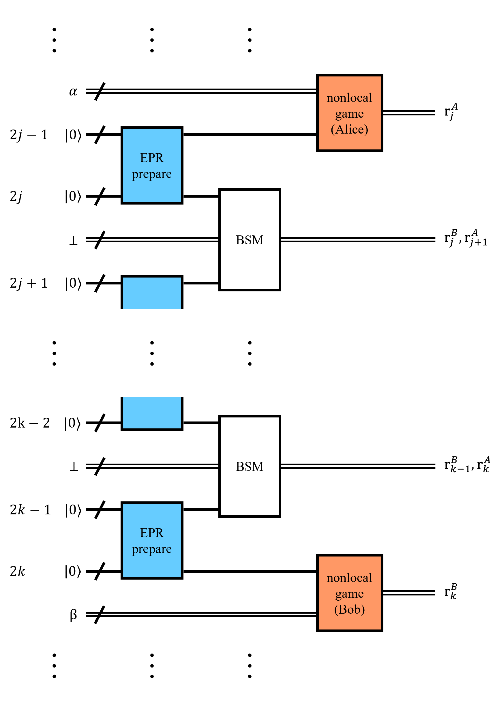
(b)

Figure 2: (a) Description of the shallow-circuit computation task $R^{8}_{N}$. (b) A quantum shallow circuit that realizes $R^{8}_{N}$. The odd-valued sites can be regarded as held by Alice, and the even-valued sites can be regarded as held by Bob. Each site consists of a set of classical wires to receive the input of $R^{8}_{N}$ and quantum wires initialized in $\ket{0}$ for three qubits. Throughout this work, we denote the classical systems by double wires and quantum systems by single wires. First, Alice and Bob prepare three pairs of Einstein-Podolski-Rosen (EPR) state, $(\ket{00}+\ket{11})/\sqrt{2}$, between their adjacent sites $(2i-1,2i),i\in\mathbb{N}^{+}$, as shown by the blue boxes. Next, given an input instance $(j,k,\alpha,\beta)$, Alice and Bob perform concatenated Bell-state measurements (BSM) between their adjacent sites $(2j,2j+1),\cdots,(2k-2,2k-1)$, as shown by the white boxes. In the end, Alice and Bob perform the perfect-winning strategy for the nonlocal game at sites $2j-1$ and $2k$ with respect to the questions $\alpha$ and $\beta$, respectively, as shown by the orange boxes.

(a)

(b)

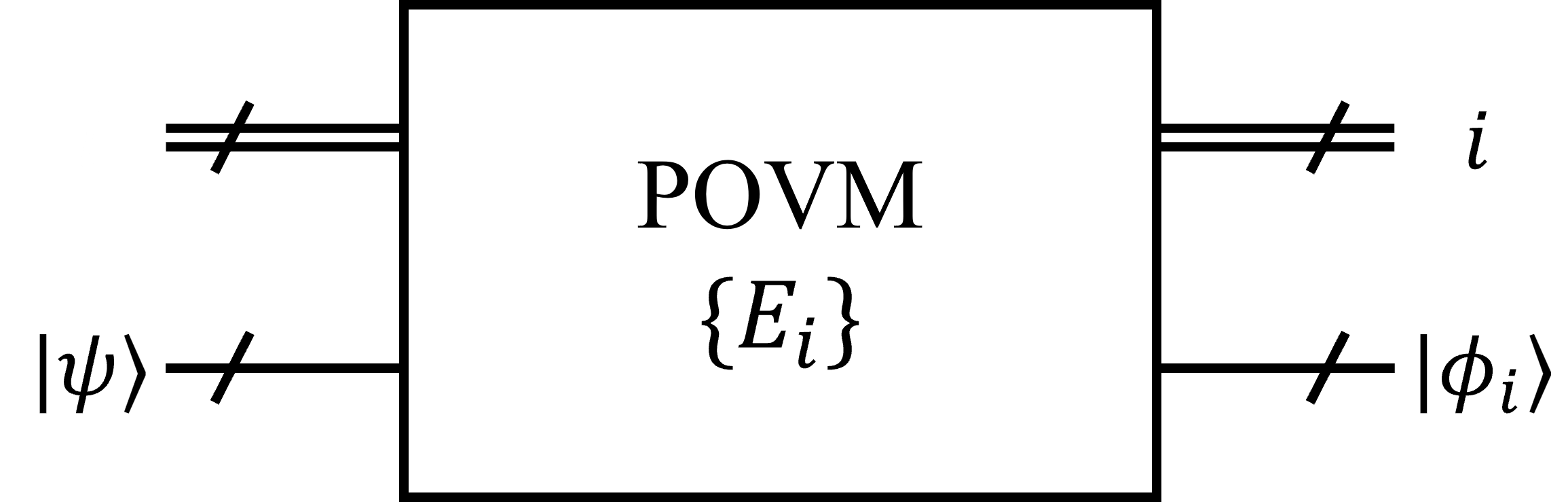
(c)

Figure 3: (a) A general $K$-bounded fan-in gate. In general, it acts on $n_{c}$ bits and $n_{q}$ qubits, with $n_{c}+n_{q}\leq K$. When $n_{c}=0$, it becomes a normal quantum gate characterized by a unitary operation. When $n_{q}=0$, it becomes a normal classical gate. (b) The classically controlled quantum gate. The classical input $i$ controls whether to apply the quantum gate $U_{i}$ to the quantum input state $\ket{\psi}$. In a $\mathsf{ClifNC}^{0}$circuit, we allow such classically controlled gate with $U_{i}$ restricted to a Clifford operation. (c) A general quantum measurement characterized by a positive operator-valued measure (POVM). The classical system acts as a register to record the measurement result. In a $\mathsf{ClifNC}^{0}$circuit, each measurement element $E_{i}$ is a mixture of stabilizer states. Equivalently, for a magic-free quantum input state $\ket{\psi}$, the post-measurement state $\ket{\phi_{i}}$ in a $\mathsf{ClifNC}^{0}$circuit still does not contain quantum magic. In this work, we simply consider projective measurements. Both (b) and (c) can be unified under the general description of (a).

III “Magic” computational advantage in shallow circuits

The nonlocal game shown in Theorem 3 separates the capabilities between a generic quantum world and the magic-free world to generate correlations. Now, we translate correlation generation into a computation task of a relation problem  and show the advantage of magic. As a reminder, the computation task is a single-user one. “Alice” and “Bob” now refer to parts of the circuit, which is merely for an intuitive thinking. In particular, one should not consider the task as a distributed computation.

Briefly speaking, a relation problem randomly selects an input bit string $z_{\mathrm{in}}$ from a set and asks the computation to output a bit string $z_{\mathrm{out}}$, such that $z_{\mathrm{out}}$ always satisfies a certain relation with respect to $z_{\mathrm{in}}$. Given a nonlocal game with size $n$, we can define a relation problem, $R_{N}^{n}$, by embedding it into a one-dimensional grid, as shown in Fig. 2. One can imagine that two experimentalists, Alice and Bob, each hold $N$ computing sites and collaborate to solve $R_{N}^{n}$. We use the capital letter $N$ for the number of computing sites to distinguish it from the underlying nonlocal game size $n$. The input of $R_{N}^{n}$ randomly specifies one site of Alice and Bob, respectively, and picks up questions in the nonlocal game, which we encode as bit strings $\alpha\in\mathcal{Q}^{A},\beta\in\mathcal{Q}^{B}$. Among the valid outputs of $R^{n}_{N}$, the specified two sites are required to output the correct answer with respect to the questions, $(\mathbf{r}_{j}^{A},\mathbf{r}_{k}^{B})=f(\alpha,\beta)$, denoted as a function of the questions, with a non-negligible probability.

In a circuit comprising $K$-bounded fan-in gates, where each gate can act on at most $K$ inputs, the value $K$ mimics the light speed for information scrambling [39]. Furthermore, if the circuit is shallow, where the circuit depth is a constant independent of the problem size, it restricts the “time” for information scrambling; hence, many sites in the circuit are “space-like” separated from each other. Alice and Bob must be capable of playing the nonlocal game between such sites to compute the relation problem successfully. Suppose the nonlocal game defining the relation problem cannot be won perfectly without a particular resource. In that case, the players must communicate to exchange information and generate the desired correlation, which takes “time.” Therefore, a shallow circuit with bounded fan-in gates should fail. On the contrary, things become different if the nonlocal game can be won perfectly: first, entanglement can be created between certain sites and then distributed between two arbitrary sites via entanglement swapping with bounded fan-in quantum gates in constant steps [25]; after sharing entanglement, the two specified sites apply the perfect winning strategy of the nonlocal game to output the correct answers of $R_{N}^{n}$. Note that quantum gates acting on near-neighbor qubits, or geometrically local gates, suffice to complete the two steps. A subtle issue is the so-called bit and phase flips in entanglement swapping, where a subsystem of $\ket{\Phi^{+}}$ may experience a rotation of a Pauli operator. One can embed the circuit outcomes in these cases to the allowed relation for the computation problem.

Applying the Mermin-Peres nonlocal game to this logic, an unconditional advantage of quantum shallow circuits over their classical counterparts has been established [25]. Considering the relation problem $R^{n}_{N}$ defined with the new BCS nonlocal game in Eq. (2), one can further expect an unconditional separation between generic quantum shallow circuits and those without magic. Here, we specify the exact meaning of these circuits. As shown in Fig. 3, a generic gate transforms a number of classical bits and qubits. The classically controlled quantum gate and the measurement can be both unified in this way. In our definition, the fan-in includes both classical bits and qubits. We call a generic quantum shallow circuit comprising general bounded fan-in gates a $\mathsf{QNC}^{0}$circuit [40]. If there is no qubit, the circuit degenerates into a classical one, called an $\mathsf{NC}^{0}$circuit [41, 17]. For the circuit without magic, the initial quantum state must be magic-free, which can be taken as $\ket{0}$ without loss of generality, the classically controlled quantum gates must be Clifford gates, and the measurements must be Pauli measurements. In this way, there is no magic in the quantum part in any step of this circuit, and we name such circuit $\mathsf{ClifNC}^{0}$.

The following theorem illustrates the separation between $\mathsf{QNC}^{0}$and $\mathsf{ClifNC}^{0}$circuits in solving the BCS relation computation problem. We fix $n=8$ here, while the result can be generalized to a general fixed value of $n$. We provide the details in the Appendix C.

Theorem 4.

Given the relation problem, $R_{N}^{8}$, and a constant integer $K\geq 14$, the following holds:

• The relation problem can be perfectly solved by a constant-depth quantum circuit with $K$-bounded fan-in geometrically local gates.

• Any circuit containing only $K$-bounded fan-in magic-free gates that solves the relation problem $R_{N}^{8}$ with probability larger than $(1+p_{\mathrm{Cli}})/2$ with $p_{\mathrm{Cli}}$ is given in Eq. (4), where the gates can be non-geometrically local, must have a circuit depth at least increasing logarithmically with respect to $N$.

Combined with previous results [24, 25], Theorem 4 shows the hierarchy of the circuit power:

$$\text{{\hbox{\mathsf{NC}^0}}}\subset\text{{\hbox{\mathsf{ClifNC}^0}}}\subset\text{{\hbox{\mathsf{QNC}^0}}}.$$ (6)

In the second part of the theorem, the logarithmic separation is tight. That is, a magic-free circuit with bounded fan-in gates can solve the problem, of which the depth grows logarithmically. For a straightforward solution, all the computing sites send their input to a fixed ancilla, which performs the nonlocal game calculation and sends back the result to the specified sites. As entanglement does not help spread the input information faster, using magic-free entanglement does not improve the result.

IV Conclusions

In summary, we discover a family of BCS nonlocal games that requires quantum magic to win perfectly and translate it into an unconditional proof of magic computation advantage. We believe other nonlocal games exist that can demonstrate magic advantage. For instance, following the method of embedding a general group into a BCS in Ref. [35], one can obtain candidate BCS nonlocal games. In Appendix D, we review the procedure. Combined with Theorem 1, one can efficiently check whether it has a perfect-winning Clifford strategy. Besides those based on the BCS, one may look for other types of nonlocal games. Note that to prove the computation advantage, the winning probability of all Clifford strategies in the nonlocal game, which can exploit infinite-dimensional quantum systems, must be upper-bounded. To perform the relation problem calculation in a realistic experiment, one shall further consider the noise and loss. For this purpose, noise-tolerant methods, such as error correction and mitigation in a shallow circuit, need to be developed. While not being the purpose of this work, by applying the “game gluing” technique [42, 43], one can combine games with different sizes in the family and construct a nonlocal game with a strict separation between the winning probabilities of classical, Clifford, and general quantum strategies. We consider this may be of an independent interest to some research. This work takes the first step in proving the computation necessity of quantum magic unconditioned on any complexity assumption. We hope our results can inspire further explorations in this direction, eventually going beyond the regime of shallow circuits and solidifying the “magic” of universal quantum computation.

All the authors contributed equally to this work.

Appendix A Preliminaries

In this section, we review preliminary concepts for this work. We assume readers are familiar with the basic notions of linear algebra, graph theory, and group theory, and the basic description of quantum systems.

In the Appendix, we overuse some letters such as $n$ when expressing the total number of items or labelling the variables; nevertheless, their meaning can be specified from the context.

A.1 Quantum magic and non-Clifford operations

We first briefly review the concept of quantum magic and related notions. For simplicity, we only consider the $n$-qubit system based on the Pauli group. Nevertheless, the results can be easily generalized to systems with a prime dimension by using the Weyl-Heisenberg algebra. Readers who are interested in the topic may refer to the Ph.D. thesis of Gottesman [5] and its following works for a more in-depth discussion.

Let us start with the definition of the Pauli observables on a single qubit:

$$\mathbb{I}=\begin{pmatrix}1&0\\ 0&1\\ \end{pmatrix},\quad\sigma_{x}=\begin{pmatrix}0&1\\ 1&0\\ \end{pmatrix},\quad\sigma_{y}=\begin{pmatrix}0&-i\\ i&0\\ \end{pmatrix},\quad\sigma_{z}=\begin{pmatrix}1&0\\ 0&-1\\ \end{pmatrix},$$ (7)

where $\mathbb{I}$ is the identity operator, and the other three observables $\sigma_{x}$, $\sigma_{y}$, and $\sigma_{z}$ are always named nontrivial Pauli observables. The $n$-qubit Pauli group is defined as the set of operators

$$\mathbb{P}_{n}=\{\pm 1,\pm i\}\times\{\mathbb{I},\sigma_{x},\sigma_{y},\sigma_{z}\}^{\otimes n},$$ (8)

together with the operator multiplication. Sometimes, one may omit the phase $\{\pm 1,\pm i\}$ and consider the $n$-qubit projective Pauli group:

$$\mathbb{P}^{\prime}_{n}=\{\mathbb{I},\sigma_{x},\sigma_{y},\sigma_{z}\}^{\otimes n}.$$ (9)

The Clifford group is defined as the normalizer of the Pauli group $\mathbb{P}_{n}$:

$$\mathbb{C}_{n}=\{C\in\mathbb{U}_{n}|\forall P\in\mathbb{P}_{n},CPC^{\dagger}\in\mathbb{P}_{n}\},$$ (10)

where $\mathbb{U}_{n}$ is the $n$-qubit unitary group. Operators in the Clifford group are called Clifford operations or gates. A highly related concept is the stabilizer state, which is generated by applying Clifford gates on the computational basis states, or equivalently the eigenstates of $\sigma_{z}^{\otimes n}$. If a state cannot be prepared in this way or by mixing stabilizer states, the state is said to contain quantum “magic” [4].

It is well known that if a quantum circuit only contains Clifford gates with the initial state being a computational basis states and measurements as Pauli observables, the measurement results can be simulated by a polynomial-size classical circuit. This is the famous Gottesman-Knill Theorem [5, 6]. Thus, this kind of circuit is deemed to be “easy” and contains no “magic.” Any circuit starting non-stabilizer states, applying non-Clifford gates, or measuring non-Pauli observables might contain magic. As magic-free circuits can be simulated classically, magic is regarded as an indispensable resource for universal quantum computation.

A.2 General binary constraint systems

For completeness, we first review the definition of a binary constraint system (BCS). A BCS consists of $n$ binary variables $v_{1},\cdots,v_{n}$ and $m$ constraints $c_{1},\cdots,c_{m}$, where each $c_{i}$ is a Boolean equation with respect to a subset of $v_{j}$’s. Note that BCS with general Boolean constrains can describe general systems of equations [42]. In a linear BCS, all the constraints are given by addition over $\mathbb{Z}_{2}$, or the parity operation over Boolean variables ranging in $\mathbb{Z}_{2}=\{0,1\}$. In the literature, such a BCS is also called a parity BCS. For convenience of a quantum generalization, it is equivalent to define the BCS over sign variables ranging in $\{+1,-1\}$. In this case, a Boolean function can be equivalently given by a multilinear function of a subset of variables on $\mathbb{R}$. For a linear BCS, the parity constraint becomes a product of the variables. In accordance with the notations in the main text, we mainly use the sign variables and denote each constraint $c_{j}$ as a multilinear function of a set of variables $\{v_{i}:i\in\mathcal{S}_{j}\}$, namely in the form of $\prod_{i\in\mathcal{S}_{j}}v_{i}=c_{j}\in\{+1,-1\}$. Nevertheless, it is sometimes more convenient to use the Boolean variables to represent a BCS. In correspondence to the sign variables,

$$\begin{split}v_{i}v_{j}=+1\Leftrightarrow v_{i}\oplus v_{j}=0,\\ v_{i}v_{j}=-1\Leftrightarrow v_{i}\oplus v_{j}=1,\\ \end{split}$$ (11)

where the LHS are the notations using sign variables and the RHS are the notations using Boolean variables. We shall specify the notations if we resort to the Boolean variables.

If a BCS has a satisfying assignment, namely a fixed assignment to the variables that satisfies all the constraint, we say it has a classical solution. Note that if all the constraints are $c_{j}=+1$, the BCS can be trivially satisfied by assigning all the variables to be $+1$. With respect to the BCS size, searching for a classical solution to a general BCS is $\mathsf{NP}$-hard. On the other hand, the problem is in $\mathsf{P}$ for linear BCS, where one can apply Gaussian elimination or the replacement method to efficiently solve the system.

The quantum generalization of a BCS is an operator-valued constraint system. The variables $v_{j}$’s are replaced with linear operators $A_{j}$’s acting on a Hilbert space $\mathcal{H}$ with a finite dimension, such that

1. Each $A_{j}$ is Hermitian with eigenvalues in $\{1,-1\}$, i.e., $A_{j}=A_{j}^{\dagger}$ and $A_{j}^{2}=\mathbb{I}$ for all $j$.

2. $A_{j}$’s satisfy all the constraints with $c_{i}$ replaced with $c_{i}\mathbb{I}$, where $\mathbb{I}$ is the identity operator on $\mathcal{H}$.

3. If $A_{i}$ and $A_{j}$ appear in the same constraint, they commute with each other, i.e., $A_{i}A_{j}=A_{j}A_{i}$.

If there exists a Hilbert space $\mathcal{H}$ with dimension $d$ and a set of linear operators following the above requirements, we say the BCS has a $d$-dimensional quantum satisfying assignment, or simply a quantum solution. As a side remark, the requirement that the operator variable acts on a finite-dimensional Hilbert space can be relaxed in several directions, including allowing an infinite dimension and limits of finite-dimensional systems. We do not discuss such generalizations and refer readers to Ref. [35, 45] for a more detailed definition.

If a BCS has a quantum solution, one can apply quantum measurements to realize it in an experiment, where they prepare independently and identically many copies of a quantum state and measure the observables in each constraint. For each constraint, the measurement results shall satisfy the relation in the fashion of classical variables. Note that the requirement for a quantum solution guarantees the validity of a joint measurement for each constraint. Due to the intrinsic randomness in quantum measurements, the same variable may take different values in different constraints. It is worth mentioning that measuring the set of observables on any state, including a maximally mixed state, generates the desired statistics for the constraints. The quantum satisfying assignment is also called a state-independent contextuality of the observables [46].

As the dimension can be arbitrary, searching for a quantum solution is undecidable [35, 34]. A helpful way of thinking is to regard the BCS as a group presentation statement [32, 47].

Definition 1 (Group presentation).

Given a set $\mathcal{S}$, let $\mathcal{F}(\mathcal{S})$ be the free group on $\mathcal{S}$ and $\mathcal{R}$ a set of words on $\mathcal{S}$, and denote the quotient group of $\mathcal{F}(\mathcal{S})$ by the smallest normal subgroup containing each element in $\mathcal{R}$ as $\langle\mathcal{S}:\mathcal{R}\rangle$. A group $G$ is said to have the presentation $\langle\mathcal{S}:\mathcal{R}\rangle$ if it is isomorphic to $\langle\mathcal{S}:\mathcal{R}\rangle$.

In the group presentation, the elements in $\mathcal{S}$ are called generators and the elements in $\mathcal{R}$ are called relators. Given a linear BCS, one can regard the constraints as a group presentation.

Definition 2 (Solution group of a linear BCS).

Given a linear BCS with $n$ binary variables $\{v_{i}\}$ and $m$ constraints $\{c_{j}\}$, the solution group of the BCS is defined as the group with the following presentation:

$$\begin{split}\Gamma=\{\{J,g_{i}:i\in[n]\}:\{g_{i}^{2}&=e,\forall i\in[n],\\ J^{2}&=e,\\ \forall j\in[m],g_{k}g_{l}&=g_{l}g_{k},\forall k,l\in\mathcal{S}_{j},\\ Jg_{i}&=g_{i}J,\forall i\in[n],\\ \prod_{i\in\mathcal{S}_{j}}g_{i}&=J^{\chi(c_{j}=-1)},\forall j\in[m]\}\},\end{split}$$ (12)

where the group element $J$ corresponds to $-1$ in the BCS, $e$ defines the identity operator of the group, and $\chi(\cdot)$ is the indicator function that takes the value $1$ if the argument is true and $0$ if the argument is false.

Note that if $J=e$, the solution group is trivial, as the assignment of all the group elements to be $e$ satisfies all the relators. On the contrary, should $J\neq e$, the solution group is non-trivial, and the group presentation corresponds to a valid operator-valued solution to the underlying BCS, as stated by the following lemma.

Lemma 1 ([47, 43]).

Given a linear BCS that defines a solution group with the group element $J$ corresponding to $-1$, if $J$ is non-trivial in some finite-dimensional representation of the solution group, then the BCS has a finite-dimensional quantum satisfying assignment. The converse is also true.

The irreducible representation of the generators in the solution group determines the quantum realization [47, 37]. Here, a representation of the group refers to a group homomorphism of the group to a set of unitary operators on a Hilbert space, and an irreducible representation refers to a representation that does not have a non-trivial group-invariant subspace [48]. For a classical solution, it can be described by the Abelian group, where all the group elements commute with each other.

As an example of linear BCS, we review the Mermin-Peres BCS, also widely known as the “magic-square” system [30, 31]. Note that one should not mistake the name “magic” with the quantum resource of magic states. The Mermin-Peres BCS involves $n=9$ variables and $m=6$ constraints. In terms of sign variables ranging in $\{+1,-1\}$, the BCS is defined as follows:

$$\begin{split}v_{1}v_{2}v_{3}&=1,\\ v_{4}v_{5}v_{6}&=1,\\ v_{7}v_{8}v_{9}&=1,\\ v_{1}v_{4}v_{7}&=1,\\ v_{2}v_{5}v_{8}&=1,\\ v_{3}v_{6}v_{9}&=-1.\end{split}$$ (13)

This BCS does not have a classical solution. On the other hand, it has a unique quantum solution over the Pauli group. We denote the operator that corresponds to $v_{i}$ as $A_{i}$ in accordance with the notations above. The quantum solution is given as follows [44, 43]:

$$\begin{split}A_{1}&=\sigma_{z}\otimes\mathbb{I},\\ A_{2}&=\mathbb{I}\otimes\sigma_{z},\\ A_{3}&=\sigma_{z}\otimes\sigma_{z},\\ A_{4}&=\mathbb{I}\otimes\sigma_{x},\\ A_{5}&=\sigma_{x}\otimes\mathbb{I},\\ A_{6}&=\sigma_{x}\otimes\sigma_{x},\\ A_{7}&=\sigma_{z}\otimes\sigma_{x},\\ A_{8}&=\sigma_{x}\otimes\sigma_{z},\\ A_{9}&=\sigma_{y}\otimes\sigma_{y},\end{split}$$ (14)

where $\otimes$ stands for the tensor product operation.

Given a BCS, one can define an associated nonlocal game [32]. In the nonlocal game, there are two cooperating players, Alice and Bob, who cannot communicate with each other once the game starts. With respect to a probability distribution, a referee randomly selects one constraint, $c_{s}$, and one variable, $v_{t}$, contained in the constraint. In our work, we always take the probability distribution to be uniform. The referee send $s$ to Alice and $t$ to Bob. Then, Alice returns an assignment to each variable $v_{i}$ in $c_{s}$ that satisfies the constraint and Bob returns an assignment to variable $v_{t}$. They win the game if and only if the assignments of Bob and Alice to $v_{t}$ are the same. This type of nonlocal game extends the well-known Clauser-Horne-Shimony-Holt (CHSH) game [49], where the underlying BCS involves two binary variables and two multi-linear constraints,

$$\begin{split}v_{1}v_{2}&=1,\\ v_{1}v_{2}&=-1.\end{split}$$ (15)

This BCS game is equivalent to the CHSH game in the sense of the probability distribution that Alice and Bob can achieve. Note that this BCS does not have either a classical solution or a quantum solution. Still, quantum strategies for the game can bring a higher winning probability than classical ones.

To maximize the winning probability, Alice and Bob can agree on a strategy for playing the game. We call a strategy is perfect if it wins with probability 1. We say Alice and Bob apply a classical strategy if they can access only shared and local randomness. In quantum theory, Alice and Bob can pre-share entanglement and apply local quantum operations. In general, when a BCS does not have a solution, it is possible that Alice assigns different values to the same variable upon different questions of constraint. However, it brings limited advantage. For classical strategies, using basic linear algebra analysis, it is not hard to prove that a BCS game has a perfect classical strategy if and only if the corresponding BCS has a solution. It follows that to decide whether a general BCS game has a perfect classical strategy is in $\mathsf{NP}\text{-hard}$ for general Boolean constraints and in $\mathsf{P}$ for linear constraints with respect to the BCS size. In the above examples, the CHSH game has a maximal winning probability of $3/4$, and the Mermin-Peres game has a maximal winning probability of $8/9$. In the quantum case, if the BCS does not have an operator-valued solution, then there does not exist a perfect winning strategy for the associated nonlocal game, and vice versa. This fact is first proved in Ref. [32]. If the BCS has a quantum solution, it is linked to a perfect quantum winning strategy in a one-to-one correspondence. Suppose the quantum solution to the BCS is given by observables $\{A_{i}\}_{i}$ acting on a $d$-dimensional system. Alice and Bob first share a maximally entangled state, $\ket{\Phi^{+}}=\sum_{i=0}^{d-1}\ket{ii}/\sqrt{d}$. When the nonlocal game starts, upon receiving the constraint $c_{s}$, Alice measures the observables $A_{i}$ belonging to the constraint, and upon receiving the variable $v_{t}$, Bob measures the transpose of the observable $A_{t}$, denoted by $A_{t}^{\mathrm{T}}$. The measurement statistics satisfy the winning condition.

For the well-known existing BCS that are solvable, it either has a classical solution, which corresponds to an Abelian group, or a quantum solution of Pauli strings as in the case of the Mermin-Peres magic square, which corresponds to the Pauli group. In Ref. [33], the author provides an efficient algorithm to determine perfect quantum solutions to a special type of linear BCS, where each variable shows up in exactly two constraints. Moreover, if such a BCS has a solution, the solution is necessarily given by Pauli strings, i.e., the solution is in the Pauli group. Following this result, it was conjectured that any linear BCS with an operator-valued satisfying assignment belongs to either of the two cases [33]. As mentioned in the main text, this conjecture has been suggested false [35, 34]. In the next section, we directly disprove this conjecture with a specific linear BCS.

Appendix B Group-Theoretic Analysis of the Binary Constraint System

In this section, we apply group-theoretic tools to analyse the properties of the proposed linear BCS in the main text.

B.1 A binary constraint system over the permutation group

We first review the BCS proposed in this work. Given an undirected complete graph $G=(V,E)$ with $n$ vertices, it defines the following variables:

1. Each vertex $v\in V$ corresponds to one variable $a_{v}$.

2. Each undirected edge, denoted by $e=(u,v)\in E$, corresponds to three variables $x_{uv},y_{uv},z_{uv}$.

3. Every two disjoint edges, denoted by $e_{1}=(u,v)\in E$ and $e_{2}=(s,t)\in E$, where $s,t,u,v$ are different vertices, correspond to

   1. one variable $b_{uv|st}\equiv b_{st|uv}$, where $b_{e_{1}e_{2}}=b_{e_{2}e_{1}}$;

   2. two variables $c_{e_{1}e_{2}}\equiv c_{uv|st}$ and $c_{e_{2}e_{1}}\equiv c_{st|uv}$, where $c_{e_{1}e_{2}}\neq c_{e_{2}e_{1}}$ in general.

Based on these variables, the BCS contains the following constraints,

$$\begin{split}a_{u}a_{v}y_{uv}&=1,\forall(u,v)\in E,\\ x_{uv}y_{uv}z_{uv}&=1,\forall(u,v)\in E,\\ x_{uv}x_{st}b_{uv|st}&=1,\forall(u,v),(s,t)\in E,\\ x_{uv}z_{st}c_{uv|st}&=1,\forall(u,v),(s,t)\in E,\\ b_{uv|st}b_{vs|ut}b_{su|vt}&=1,\forall(u,v),(s,t)\in E,\\ c_{uv|st}c_{vs|ut}c_{su|vt}&=1,\forall(u,v),(s,t)\in E,\\ \prod_{v\in V}a_{v}&=-1.\end{split}$$ (16)

For a nontrivial BCS, the system size is at least $n=4$. If the BCS has a solution, then the other variables can be generated by $a^{\prime}$s and $x^{\prime}$s. For convenience, we label the vertices with natural numbers from $1$ to $n$. For each vertex $v$ and each edge $(u,v),u\neq v$, we can use transpositions between elements in the set $[2n]$ to represent the generators, where $a_{v}=(2v-1\ 2v)$ and $x_{uv}=(2u-1\ 2v-1)(2u\ 2v)$. Here, $(i\ j)$ represents a transposition between $i$ and $j$. We have the following results for the BCS.

Theorem 5.

For any BCS of the above form with $n\in 2\mathbb{N}+5=\{5,7,9,\cdots\}$, it has a classical solution.

Proof.

When $n\in 2\mathbb{N}+5$, the BCS can be satisfied by assigning all the variables $a_{v}$’s to be $-1$ and all the other variables to be $1$. ∎

Theorem 6.

When $n=4$, this BCS has a two-qubit Pauli-string solution. On the other hand, the BCS does not have a classical solution or a single-qubit Pauli solution in this case.

Proof.

The BCS having no classical solution can be directly checked by solving the BCS on the binary field. By using the fact that there is no state-independent contextuality in a qubit system, one can prove that the BCS does not have a single-qubit Pauli solution either [50, 51, 52]. Later, we prove this statement under the context of linear BCS.

For the former statement, here is one construction of the two-qubit Pauli-string solution. We abbreviate the Pauli operators $\mathbb{I},\sigma_{x},\sigma_{y},\sigma_{z}$ as $I,X,Y,Z$, respectively, and omit the tensor-product operator in the expressions.

$a_{1}$	$a_{2}$	$a_{3}$	$a_{4}$
$-ZZ$	$II$	$ZI$	$IZ$
$x_{12}$	$x_{13}$	$x_{14}$	$x_{23}$	$x_{24}$	$x_{34}$
$-YY$	$XI$	$IX$	$II$	$II$	$ZZ$
$y_{12}$	$y_{13}$	$y_{14}$	$y_{23}$	$y_{24}$	$y_{34}$
$-ZZ$	$-IZ$	$-ZI$	$ZI$	$IZ$	$ZZ$
$z_{12}$	$z_{13}$	$z_{14}$	$z_{23}$	$z_{24}$	$z_{34}$
$-XX$	$-XZ$	$-ZX$	$ZI$	$IZ$	$II$
$b_{12|34}$	$b_{13|24}$	$b_{14|23}$
$XX$	$XI$	$IX$
$c_{12|34}$	$c_{13|24}$	$c_{14|23}$	$c_{34|12}$	$c_{24|13}$	$c_{23|14}$
$-YY$	$XZ$	$ZX$	$YY$	$-XZ$	$-ZX$

Table 1: A two-qubit Pauli-string solution for the BCS when $n$ = $4$.

∎

Theorem 7 (A special case of the results in Ref. [50, 51, 52]).

If a linear BCS has a single-qubit operator-valued solution, then it has a classical solution.

Proof.

Two-dimensional matrices have such a special property: Suppose $A,B\in\mathbb{C}^{2\times 2}$ and $[A,B]=AB-BA=0$. At least one of the following cases would happen (1) $A=c\mathbb{I}$ for some $c\in\mathbb{C}$; (2) $B=c\mathbb{I}$ for some $c\in\mathbb{C}$; (3) $A=cB$ for some $c\in\mathbb{C}$. Therefore, all two-dimensional matrices that are not proportional to the identity matrix $\mathbb{I}$ can be classified into different equivalence classes, with elements in a class proportional to each other.

Given a single-qubit operator-valued solution, denote the first equivalent class as $\{c_{1}O,c_{2}O,\cdots|c_{1},c_{2},\cdots=\pm 1\}$ where $O\neq\pm\mathbb{I}$ and $O^{2}=\mathbb{I}$. Substituting $\{c_{1}O,c_{2}O,\cdots|c_{1},c_{2},\cdots=\pm 1\}$ with $\{c_{1}\mathbb{I},c_{2}\mathbb{I},\cdots|c_{1},c_{2},\cdots=\pm 1\}$ and not changing other variables also provides a solution. This is because (1) variables in different equivalent classes do not show up in the same constraint; (2) the constraints among the variables proportional to $\mathbb{I}$ and in the first equivalent class are not violated after the substitution. Similarly, we can set all variables proportional to $\mathbb{I}$ to give a solution. The proportional coefficient is a valid classical solution. ∎

Theorem 8.

For any BCS of the above form with $n\in 2\mathbb{N}+6=\{6,8,10,\cdots\}$, it does not have a Pauli-string solution.

Proof.

Later we shall present a general method to determine whether a general linear BCS has a Pauli-string solution, where the current result can be regarded as a special case. Nevertheless, here we present a graph-based proof specific to this BCS, which is more illustrative.

We first specify the commutation properties of Pauli strings. The Pauli group elements are either anti-commuting, like $\{X,Z\}=XZ+ZX=0$, or commuting, like $[X\otimes X,Z\otimes Z]=(X\otimes X)(Z\otimes Z)-(Z\otimes Z)(X\otimes X)=0$. Therefore, if we swap any two operators in a multiplication of some Pauli-string operators, the operator value of the multiplication would at most differ with a sign.

Now we prove the theorem by contradiction. Assume the BCS described in the theorem has a Pauli-string solution. Without loss of generality, with respect to the correspondence between the BCS variables and vertices in a fully connected undirected graph in Fig. 3(c), let us consider the sets of variables and constraints corresponding to a subgraph with five vertices, labeled with $1$ through $5$. For the quadrangle $\{1,2,4,5\}$, we have the equation $b_{12|45}b_{24|15}b_{41|25}=\mathbb{I}$. Substituting all the $b$-type variables by $x_{uv}x_{st}b_{uv|st}=\mathbb{I}$, we have

$$x_{12}x_{45}x_{24}x_{15}x_{41}x_{25}=\mathbb{I}.$$ (17)

Similarly, for the quadrangles $\{1,3,4,5\}$ and $\{2,3,4,5\}$, we have the equations

$$x_{13}x_{45}x_{34}x_{15}x_{41}x_{35} =\mathbb{I}.$$ (18)

$$x_{23}x_{45}x_{34}x_{25}x_{42}x_{35} =\mathbb{I}.$$ (19)

Next, by multiplying the left and right sides of Eqs. (17)(18) and (19), respectively, swapping the order of the variables, and eliminating the adjacent two variables that are the same, we get

$$x_{12}x_{13}x_{23}x_{45}=\pm\mathbb{I},$$ (20)

where “$\pm$” denotes that either case would happen. In this step, we have used the commutation properties of Pauli strings. In other words,

$$x_{45}\in\{\pm x_{12}x_{13}x_{23}\}.$$ (21)

As a reminder, $x_{uv}$ and $x_{vu}$ represent the same variable. Note that there is nothing special about the choice of $x_{45}$ among the variables, and a similar result can be obtained with an arbitrary specification of a subgraph with five vertices. For instance, we can get

$$x_{46}\in\{\pm x_{12}x_{13}x_{23}\}.$$ (22)

Combining the above two equations, we have $x_{45}=\pm x_{46}$. For $n\geq 6$, following the above procedure and enumerating all such identities, one shall find that all the $x$-type variables differ from each other up to a sign, i.e., $x_{uv}\in\{\pm x\}$ for all $(u,v)\in E$. Thus we can assume that $x_{uv}=x^{\prime}_{uv}x$ where $x^{\prime}_{uv}\in\{\pm 1\}$.

Following the specification of the $x$-type variables, for any four distinct vertices $u,v,s,t\in V$, we have the following expressions:

$$\begin{split}b_{uv|st}&=x_{uv}x_{st}=x^{\prime}_{uv}x^{\prime}_{st}\mathbb{I},\\ c_{uv|st}&=x_{uv}z_{st}=x_{uv}x_{st}y_{st}=x^{\prime}_{uv}x^{\prime}_{st}y_{st}=x^{\prime}_{uv}x^{\prime}_{st}a_{s}a_{t}.\end{split}$$ (23)

Consequently,

$$\begin{split}b_{uv|st}b_{vs|ut}b_{su|vt}&=x^{\prime}_{uv}x^{\prime}_{st}x^{\prime}_{vs}x^{\prime}_{ut}x^{\prime}_{su}x^{\prime}_{vt}=1,\\ c_{uv|st}c_{vs|ut}c_{su|vt}&=x^{\prime}_{uv}x^{\prime}_{st}x^{\prime}_{vs}x^{\prime}_{ut}x^{\prime}_{su}x^{\prime}_{vt}a_{s}a_{t}a_{u}a_{t}a_{v}a_{t}=1.\end{split}$$ (24)

Note that all the $a$-type variables commute with each other, since they simultaneously appear in the last equation of the BCS. We hence derive that $a_{u}a_{v}a_{s}a_{t}=1$ for all four distinct vertices $u,v,s,t\in V$, which is equivalent to

$$a_{u}=a_{v}a_{s}a_{t}.$$ (25)

By applying a similar argument as for the $x$-type variables, we shall find that all the $a$-type variables are identical, i.e., $a_{v}\equiv a,\forall v\in V$. This contradicts the constraint $\prod_{v\in V}a_{v}=-1$ when $n$, the number of vertices, is even. Therefore, the BCS of the above form with $n\in 2\mathbb{N}+6$ does not have a Pauli-string solution. ∎

Theorem 9.

For any BCS of the above form with $n\geq 4$, label the vertices from $1$ to $n$. The BCS has a solution over the centralizer group of element $J=(1\ 2)(3\ 4)\cdots(2n-1\ 2n)$ in the permutation group $S_{2n}$.

Proof.

Consider $x_{(u,v)}=(2u-1\ 2v-1)(2u\ 2v)$, $a_{v}=(2v-1\ 2v)$, and all the other variables generated by them. One can easily check that the assignment satisfies the constraints. As $J$ does not map to the identity element of the group, this is a non-trivial quantum solution following Lemma 1. The solution group corresponds to the centralizer of $J$ in the permutation group, given by

$$C_{J}=S_{n}\ltimes\mathbb{Z}_{2}^{n},$$ (26)

which is the semi-product of the permutation group $S_{n}$ generated by $x_{(u,v)}$, and an Abelian group $\mathbb{Z}_{2}^{n}$ generated by $a_{v}$. ∎

Now we solve the irreducible representations of the solution, which gives the quantum realizations. We have the following theorem.

Theorem 10.

An irreducible representation of $S_{n}\ltimes\mathbb{Z}_{2}^{n}$ can be labeled by $\left(m,\theta^{(m)},\rho^{(n-m)}\right)$ where $m$ is an integer in $[0,n]$, $\theta^{(m)}$ and $\rho^{(n-m)}$ are two irreducible representations of permutation groups $S_{m}$ and $S_{n-m}$, respectively. Given label $\left(m,\theta^{(m)},\rho^{(n-m)}\right)$, we first get an irreducible representation of group $S_{m}\times S_{n-m}\ltimes\mathbb{Z}_{2}^{n}$, which is given by

$$\begin{split}\phi^{(m,\theta,\rho)}:S_{m}\times S_{n-m}\ltimes\mathbb{Z}_{2}^{n}&\rightarrow M_{\dim\theta^{(m)}\times\dim\rho^{(n-m)}}(\mathbb{R})\\ x\in S_{m},y\in S_{n-m},z\in\mathbb{Z}_{2}^{n},(x,y,z)&\mapsto\theta^{(m)}(x)\otimes\rho^{(n-m)}(y)\otimes\varphi^{(m)}(z).\end{split}$$ (27)

Here, $\varphi^{(m)}$ is an irreducible representation of $\mathbb{Z}_{2}^{n}$ such that for any element $z=(z_{1},z_{2},\cdots,z_{n})\in\mathbb{Z}_{2}^{n}$ where $\forall j,z_{j}\in\{0,1\}$,

$$\varphi^{(m)}(z)=\prod_{j=1}^{m}(-1)^{z_{j}}.$$ (28)

The irreducible representation of $S_{n}\ltimes\mathbb{Z}_{2}^{n}$ labeled by $\left(m,\theta^{(m)},\rho^{(n-m)}\right)$, denoted as $\Phi^{(m,\theta,\rho)}$, is the induced representation of $\phi^{(m,\theta,\rho)}$. Specifically, one first finds the left coset of $S_{m}\times S_{n-m}\ltimes\mathbb{Z}_{2}^{n}$ in $S_{n}\ltimes\mathbb{Z}_{2}^{n}$, given by

$$\left\{g_{1}S_{m}\times S_{n-m}\ltimes\mathbb{Z}_{2}^{n},g_{2}S_{m}\times S_{n-m}\ltimes\mathbb{Z}_{2}^{n},\cdots,g_{\binom{n}{m}}S_{m}\times S_{n-m}\ltimes\mathbb{Z}_{2}^{n}\right\},$$ (29)

where $\left\{g_{1},g_{2},\cdots,g_{\binom{n}{n}}\right\}$ are representative elements and $g_{1}$ is the identity. Then, the induced representation $\Phi^{(m,\theta,\rho)}$ is defined on the bases $\left\{g_{i}\vec{e}_{j}|1\leq i\leq\binom{n}{m},1\leq j\leq\dim\phi^{(m,\theta,\rho)}\right\}$ where $\vec{e}_{j}$ is a basis of the representation space of $\phi^{(m,\theta,\rho)}$. That is, for any element $g\in S_{n}\ltimes\mathbb{Z}_{2}^{n}$, suppose that $gg_{i}\in g_{\sigma(i)}S_{m}\times S_{n-m}\ltimes\mathbb{Z}_{2}^{n}$ and set $h_{i}=g_{\sigma(i)}^{-1}gg_{i}$ where $\sigma$ is a permutation on $\left\{1,2,\cdots,\binom{n}{m}\right\}$, then

$$\Phi^{(m,\theta,\rho)}(g)=\left(\Pi_{\sigma}\otimes\mathbb{I}_{\dim\phi^{(m,\theta,\rho)}}\right)\left(\bigoplus_{i=1}^{n}\phi^{(m,\theta,\rho)}(h_{i})\right).$$ (30)

Here, $\Pi_{\sigma}$ is a permutation matrix defined on the computational basis $\ket{1},\ket{2},\cdots,\ket{\binom{n}{m}}$ and transforms $\ket{i}$ to $\ket{\sigma(i)}$.

Proof.

This theorem is a direct corollary of Proposition 25 in [48]. To get an irreducible representation of $C_{J}=S_{n}\ltimes\mathbb{Z}_{2}^{n}$, we start from the irreducible representation of $\mathbb{Z}_{2}^{n}$. Note that $\mathbb{Z}_{2}^{n}=\langle a_{1}\rangle\times\langle a_{2}\rangle\times\cdots\times\langle a_{n}\rangle$ is generated by $n$ two-order elements $a_{1},a_{2},\cdots,a_{n}$. Any irreducible representation of $\mathbb{Z}_{2}^{n}$ can be labeled by a vector with length $n$, like $(1,-1,\cdots,1)$, denoting the values that $n$ generators would be mapped to in the representation. Meanwhile, we call two irreducible representations equivalent if they can be mutually transformed via $S_{n}$. In other words, two irreducible representations are equivalent if and only if the corresponding vectors have the same number of -1. To obtain an irreducible representation of $C_{J}$, we only need to consider inequivalent irreducible representations of $\mathbb{Z}_{2}^{n}$ under the transformation of $S_{n}$. Without loss of generality, we choose these irreducible representations as $(1,1,\cdots,1)$, $(-1,1,\cdots,1)$, $(-1,-1,\cdots,1)$, and $\cdots$, $(-1,-1,\cdots,-1)$ and label them with the number of -1, that is, $\{0,1,\cdots,n\}$.

For a number $m\in\{0,1,\cdots,n\}$, we get an irreducible representation of $\mathbb{Z}_{2}^{n}$, denoted as $\varphi^{(m)}$, mapping the generators $a_{i}$ to $\varphi^{(m)}(a_{i})=(-1)^{\mathbbm{1}_{i\leq m}}$. Then, we consider a subgroup of $S_{n}$, such that any element $h$ in this subgroup satisfies $\forall z\in\mathbb{Z}_{2}^{n}$,

$$\varphi^{(m)}(gzg^{-1})=\varphi^{(m)}(z),$$ (31)

or equivalently, $1\leq i\leq n$,

$$\varphi^{(m)}(ga_{i}g^{-1})=\varphi^{(m)}(a_{i}).$$ (32)

Clearly, this subgroup must be $S_{m}\times S_{n-m}$. Then, one can define the irreducible representation of $S_{m}\times S_{n-m}\ltimes\mathbb{Z}_{2}^{n}$ as

$$\begin{split}\phi^{(m,\theta,\rho)}:S_{m}\times S_{n-m}\ltimes\mathbb{Z}_{2}^{n}&\rightarrow M_{\dim\theta^{(m)}\times\dim\rho^{(n-m)}}(\mathbb{R})\\ x\in S_{m},y\in S_{n-m},z\in\mathbb{Z}_{2}^{n},(x,y,z)&\mapsto\theta^{(m)}(x)\otimes\rho^{(n-m)}(y)\otimes\varphi^{(m)}(z),\end{split}$$ (33)

where $\theta^{(m)}$ and $\rho^{(n-m)}$ are two irreducible representations of permutation groups $S_{m}$ and $S_{n-m}$, respectively. Note that $\phi^{(m,\theta,\rho)}$ is a well-defined group homomorphism due to the condition of Eq. (31). Proposition 25 in [48] tells us that any irreducible representation of $S_{n}\ltimes\mathbb{Z}_{2}^{n}$ can be constructed by the induced representation of $\phi^{(m,\theta,\rho)}$ by traversing $m$, $\theta$, and $\rho$. Proof is done. ∎

For a perfect strategy of the non-local game, the element $J$ must be mapped to a non-identity element. Note that any element in $C_{J}$ commutes with $J$. Via Theorem 10, one can obtain the following result:

$$\begin{split}\Phi^{(m,\theta,\rho)}(J)&=\varphi^{(m)}(J)\mathbb{I}_{\dim\Phi}\\ &=\varphi^{(m)}\left(\prod_{i=1}^{n}a_{i}\right)\mathbb{I}_{\dim\Phi}\\ &=\prod_{i=1}^{n}\varphi^{(m)}(a_{i})\mathbb{I}_{\dim\Phi}\\ &=(-1)^{\mod(m,2)}\mathbb{I}_{\dim\Phi},\end{split}$$ (34)

where $\dim\Phi=\binom{n}{m}\dim\phi=\binom{n}{m}\dim\theta^{(m)}\dim\rho^{(n-m)}\geq\binom{n}{m}$. Thus, $\Phi^{(m,\theta,\rho)}(J)$ corresponds to a perfect measurement strategy if and only if $m$ is odd. The smallest dimension of the quantum system for a perfect strategy is $n$ when $m=1$ or $m=n-1$ and $\dim\theta^{(m)}=\dim\rho^{(n-m)}=1$.

The quantum realization of the BCS in Eq. (16) is not unique. The underlying reason is that unlike the Pauli group, the permutation group has more than one inequivalent irreducible representations [48]. For $n=8$, which is the smallest size for a non-trivial result where there is not a Pauli-string solution to the BCS, we consider the case where $m=1$ and $\theta$ and $\rho$ are both trivial representations, in which the dimension of the quantum system is $8$. It implies that the corresponding non-local game can be realized with only $3$ EPR pairs. The representations of the generators are given by the following:

$$a_{1}=\begin{pmatrix}-1&0&\cdots&0\\ 0&1&\cdots&0\\ \vdots&\vdots&\ddots&\vdots\\ 0&0&\cdots&1\end{pmatrix},a_{2}=\begin{pmatrix}1&0&\cdots&0\\ 0&-1&\cdots&0\\ \vdots&\vdots&\ddots&\vdots\\ 0&0&\cdots&1\end{pmatrix},\cdots,a_{8}=\begin{pmatrix}1&0&\cdots&0\\ 0&1&\cdots&0\\ \vdots&\vdots&\ddots&\vdots\\ 0&0&\cdots&-1\end{pmatrix},$$ (35)

$$x_{12}=\begin{pmatrix}0&1&0&\cdots&0\\ 1&0&0&\cdots&0\\ 0&0&1&\cdots&0\\ \vdots&\vdots&\vdots&\ddots&\vdots\\ 0&0&0&\cdots&1\end{pmatrix},x_{13}=\begin{pmatrix}0&0&1&\cdots&0\\ 0&1&0&\cdots&0\\ 1&0&0&\cdots&0\\ \vdots&\vdots&\vdots&\ddots&\vdots\\ 0&0&0&\cdots&1\end{pmatrix},\cdots,x_{18}=\begin{pmatrix}0&0&0&\cdots&1\\ 0&1&0&\cdots&0\\ 0&0&1&\cdots&0\\ \vdots&\vdots&\vdots&\ddots&\vdots\\ 1&0&0&\cdots&0\end{pmatrix}.$$ (36)

From the expression of the generators, we can see that the measurement observables do not belong to the Pauli group and need magic to realize. Following the same derivation, one can prove that the smallest non-trivial irreducible representation of the solution to the BCS defined over $n$ vertices requires an $n$-dimensional system. Thus, we obtain an upper bound of the smallest number of qubits to win the non-local game.

Corollary 1.

The smallest number of qubits to win the associated nonlocal game of Eq. (16) is $2\log n$.

B.2 Capabilities of Clifford strategies in the nonlocal game

In proving the “magic” advantage in shallow circuit quantum computation, we need to specify the capabilities of Clifford strategies in the nonlocal BCS game. Thanks to the algebraic structure of BCS, we can use mature techniques from linear algebra to obtain quantitative results.

Suppose the players in a nonlocal game are restricted to Clifford operations only, or that they do not have access to quantum magic resources. In this case, the most general strategy they can apply to playing the nonlocal game is as follows:

• Before the nonlocal game starts:

  1. Alice and Bob prepares an $n$-qubit state and initialize it in $\ket{0}$.

  2. Alice and Bob apply joint Clifford operations and Pauli-string measurements to the state and evolve it into an entangled state $\rho_{AB}$, where the subscripts denote the subsystems they each will hold in the game.

• After the nonlocal game starts: Alice and Bob each applies Pauli-string measurements to their own quantum system.

In our discussions, we allow an arbitrarily large $n$. Using a convexity argument, we know that a mixed state does not bring any advantage to Alice and Bob in winning the nonlocal game, and we can hence take $\rho_{AB}$ as a pure state $\ket{\psi}$ without loss of generality. By further applying the Schmidt decomposition result, a pure state can be written as

$$\ket{\psi}=\sum_{i=0}^{d-1}\alpha_{i}\ket{ii},$$ (37)

where $\forall i,\alpha_{i}\geq 0$, and $\sum_{i=0}^{d-1}\alpha_{i}^{2}=1$. Note that the maximally entangled state, which is

$$\ket{\Phi^{+}}=\sum_{i=0}^{d-1}\frac{1}{\sqrt{d}}\ket{ii},$$ (38)

can be prepared by applying control-NOT operations to $\ket{0}$, which is a Clifford operation. Therefore, a general bipartite entangled state $\ket{\psi}$ shared by Alice and Bob can only be linked with $\ket{\Phi^{+}}$ with a Clifford operation, i.e., $\ket{\psi}=U_{C}\ket{\Phi^{+}}$.

Based upon the above observations, we discuss the capabilities of Clifford operations in playing a parity BCS nonlocal game. In demonstrating the magic advantage, we are interested in the parity BCS that do not have a Pauli-string quantum satisfying assignment. We have the following result for these instances.

Theorem 11.

Suppose a parity BCS does not have a satisfying assignment with Pauli-string observables. Then, for any Clifford strategy, there exist a constraint labelled by $c_{s}$ and a variable in it labelled by $v_{t}$, where the probability that the assignments of Alice and Bob to $v_{t}$ under the constraint $c_{s}$ are identical does not exceed $1/2$.

Proof.

In the first part of the proof, we prove the case where Alice and Bob initially share a maximally entangled state $\ket{\Phi^{+}}$ in Eq. (38) of an arbitrary dimension and then generalize the result to general Clifford strategies. In the BCS nonlocal game, without loss of generality, upon receiving the constraint labelled by $s$, Alice shall measure a set of commuting Pauli-string observables that return a satisfying assignment to the constraint, since a failure in satisfying the constraint results in a loss in the nonlocal game. On the other hand, the observables that she measures for the same variable, e.g., $v_{t}$, in different constraints can be different. To specify her strategy, we denote the observable Alice measures for vairable $v_{t}$ in the constraint $c_{s}$ as $A_{t}^{(s)}$. On Bob’s side, we denote the observable he measures for variable $v_{t}$ as $B_{t}$.

Now, suppose Alice and Bob initially share the maximally entangled state $\ket{\Phi^{+}}$. Assume there exists a Clifford strategy, such that $\forall s,t$,

$$\bra{\Phi^{+}}A_{t}^{(s)}\otimes B_{t}\ket{\Phi^{+}}>0.$$ (39)

Since Alice and Bob apply a Clifford strategy, $A_{t}^{(s)}$ and $B_{t}$ are both Pauli strings, so is $A_{t}^{(s)}B_{t}^{\mathrm{T}}$. Using the property of $\ket{\Phi^{+}}$, the left-hand side of the above equation equals $\bra{\Phi^{+}}A_{t}^{(s)}B_{t}^{\mathrm{T}}\otimes\mathbb{I}\ket{\Phi^{+}}=\tr(A_{t}^{(s)}B_{t}^{\mathrm{T}})/d$, where $d$ is the system dimension. Since $A_{t}^{(s)}B_{t}^{\mathrm{T}}$ is a Pauli string, we have $\tr(A_{t}^{(s)}B_{t}^{\mathrm{T}})/d\in\{0,\pm 1\}$. According to our assumption, we conclude that $A_{t}^{(s)}=B_{t}^{\mathrm{T}}$ and $\bra{\Phi^{+}}A_{t}^{(s)}\otimes B_{t}\ket{\Phi^{+}}=1$ for all $s,t$. Besides,

$$\begin{split}\bra{\Phi^{+}}A_{t}^{(s_{1})}A_{t}^{(s_{2})}\otimes\mathbb{I}\ket{\Phi^{+}}&=\bra{\Phi^{+}}(A_{t}^{(s_{1})}\otimes\mathbb{I})(A_{t}^{(s_{2})}\otimes\mathbb{I})\ket{\Phi^{+}}\\ &=\bra{\Phi^{+}}(A_{t}^{(s_{1})}\otimes\mathbb{I})(A_{t}^{(s_{2})}\otimes\mathbb{I})\ket{\Phi^{+}}\bra{\Phi^{+}}(\mathbb{I}\otimes B_{t})(\mathbb{I}\otimes B_{t})\ket{\Phi^{+}}\\ &\geq\bra{\Phi^{+}}A_{t}^{(s_{1})}\otimes B_{t}\ket{\Phi^{+}}\bra{\Phi^{+}}A_{t}^{(s_{2})}\otimes B_{t}\ket{\Phi^{+}}\\ &>0,\end{split}$$ (40)

which holds for all $s_{1},s_{2}$ and $t$. In the third line, we apply the Cauchy-Schwarz inequality. The only value that the above equation can take is hence $1$, indicating that $A_{t}^{(s_{1})}=A_{t}^{(s_{2})}$. Thus we can omit the superscript $(s)$.

Since the linear BCS does not have a satisfying assignment with Pauli-string observables, we can use the commutation properties of Pauli operators and the substitution method and derive an expression $A_{t_{1}}A_{t_{2}}\cdots A_{t_{m}}=-\mathbb{I}$ for a set of variables that leads to a contradiction of $\mathbb{I}=-\mathbb{I}$. The proof of this statement shall be given in Corollary 2 in Appendix D.2. Therefore, for any Clifford strategy, there exists a particular pair of inputs $s,t$ such that $\bra{\Phi^{+}}A_{t}^{(s)}\otimes B_{t}\ket{\Phi^{+}}\leq 0$. Consequently,

$$\Pr[\text{win}\mid s,t]=\frac{1}{2}\left(1+\bra{\Phi^{+}}A_{t}^{(s)}\otimes B_{t}\ket{\Phi^{+}}\right)\leq\frac{1}{2}.$$ (41)

Therefore, the average winning probability of the game is

$$\Pr[\text{win}]=\sum_{s^{\prime},t^{\prime}}\Pr[\text{win}|s^{\prime},t^{\prime}]\Pr[s^{\prime},t^{\prime}]\leq 1-\frac{1}{2}\Pr[s,t].$$ (42)

In the second part of the proof, we use the definition of Clifford operations that map a Pauli-string observable to a Pauli-string observable. For any initial state $\ket{\psi}$ that Alice and Bob may share in advance, it is linked with $\ket{\Phi^{+}}$ via a Clifford operation $U_{C}$. Then for any Pauli-string observables $A_{t},B_{t}$,

$$\bra{\psi}A_{t}\otimes B_{t}\ket{\psi}=\bra{\Phi^{+}}U_{C}^{\dagger}(A_{t}\otimes B_{t})U_{C}\ket{\Phi^{+}}\equiv\bra{\Phi^{+}}A_{t}^{\prime}\otimes B_{t}^{\prime}\ket{\Phi^{+}},$$ (43)

where $A_{t}^{\prime}$ and $B_{t}^{\prime}$ are also Pauli-string observables that adapt to the systems of Alice and Bob, respectively. Then, either $\{A_{t}^{\prime}\}$ fails in yielding a satisfying assignment to one of the constraints, or the proof dates back to the first part. This finishes the proof. ∎

Theorem 11 links the upper bound of the winning probability of the BCS nonlocal game by Clifford strategies with the game size. Consider the BCS game we construct through Eq. (16). We denote the set of questions for Alice as $\tilde{\mathcal{Q}}_{A}$, namely the BCS constraints, and the set of questions for Bob as $\tilde{\mathcal{Q}}_{B}$, namely the BCS variables. In the following tables, we give the expressions to calculate the set sizes and provide the concrete numbers for the BCS with $n=8$. For the BCS game of size $n$ with uniformly distributed questions, one may obtain a direct upper bound on the average winning probability of Clifford strategies as $1-1/(2[3(|\tilde{\mathcal{Q}}_{A}|-1)+n])$, noticing that the constraint $\prod_{v\in\mathcal{V}}a_{v}=-1$ comprises $n$ variables, while each of the other constraints consist of three variables.

constraint format	$aa^{\prime}y=1$	$xyz=1$	$xx^{\prime}b=1$	$xzc=1$	$bb^{\prime}b^{\prime\prime}=1$	$cc^{\prime}c^{\prime\prime}=1$	$\prod a=-1$	total
expression	$\binom{n}{2}$	$\binom{n}{2}$	$\binom{n}{4}\cdot 3$	$\binom{n}{4}\cdot 3\cdot 2$	$\binom{n}{4}$	$\binom{n}{4}\cdot 4$	$1$	$|\tilde{\mathcal{Q}}_{A}|$
number	$28$	$28$	$210$	$420$	$70$	$280$	$1$	$1037$

Table 2: Number of constraints in the BCS game.

variable type	$a$	$x$	$y$	$z$	$b$	$c$	total
expression	$n$	$\binom{n}{2}$	$\binom{n}{2}$	$\binom{n}{2}$	$\binom{n}{4}\cdot 3$	$\binom{n}{4}\cdot 3\cdot 2$	$|\tilde{\mathcal{Q}}_{B}|$
number	$8$	$28$	$28$	$28$	$210$	$420$	$722$

Table 3: Number of variables in the BCS game.

Appendix C 1D Magic BCS Relation Problem

In this part, we introduce the relation problem in detail by embedding the BCS nonlocal game into a one-dimensional grid. We will prove Theorem 4, showing this problem can be solved by a generic constant-depth quantum circuit with only bounded fan-in gates, while any magic-free circuit requires a circuit depth that increases at least logarithmically to the input size. For simplicity, we consider the non-trivial BCS game with size $n=8$, of which the quantum realization requires the least number of qubits, namely three pairs of qubits. One can consider other values of $n$, where the proofs are similar.

Before we commence, we slightly modify the underlying BCS defined in Eq. (16). In the BCS, all the constraints consists of three variables except for $\prod_{v\in\mathcal{V}}a_{v}=-1$, which consists of $n$ variables. For this $n$-variable constraint, we can introduce $(n-3)$ new variables and turn it into an equivalent set of $(n-2)$ constraints with three variables each. That is, we introduce new variables $a_{12},a_{123},\cdots,a_{1\cdots n-2}$ and convert the constraint as

$$a_{1}a_{2}a_{3}\cdots a_{n}=-1\quad\Longleftrightarrow\quad\left\{\begin{array}[]{rl}a_{1}a_{2}a_{12}&=1\\ a_{12}a_{3}a_{123}&=1\\ \cdots\\ a_{1\cdots n-3}a_{n-2}a_{1\cdots n-2}&=1\\ a_{1\cdots n-2}a_{n-1}a_{n}&=-1.\end{array}\right.$$ (44)

Note that the commutation requirement between variables in each constraint of the BCS is preserved in this conversion. Denote the set of constraints in the modified BCS as $\mathcal{Q}_{A}$. Suppose the original BCS with size $n$ consists of $|\tilde{\mathcal{Q}}_{A}|$ constraints. Then, in the modified BCS nonlocal game, there are $3|\mathcal{Q}_{A}|$ sets of questions, with $|\mathcal{Q}_{A}|=|\tilde{\mathcal{Q}}_{A}|+n-3$. For the case of $n=8$, by applying Theorem 11, we have the following result.

Lemma 2.

In the modified BCS game with $n=8$, suppose the questions are picked up uniformly at random. Then, the maximal winning probability for all Clifford strategies is upper-bounded by

$$p_{\mathrm{Cli}}\leq 1-\frac{1}{6252}.$$ (45)

Now we introduce the relation problem $R_{N}$, which is labeled with a number $N$ representing the problem size. One can assume that two players, Alice and Bob, collaborate with each other to solve $R_{N}$. The input and output of $R_{N}$ are given as follows.

1. Input: in each round, Alice and Bob are given a question,

   $$q=(\alpha_{1},\cdots,\alpha_{N},\beta_{1},\cdots,\beta_{N}),\alpha_{i}\in\mathcal{Q}^{A}\cup\{\perp\},\beta_{i}\in\mathcal{Q}^{B}\cup\{\perp\},$$ (46)

   where $q$ stands for “question”, $\alpha_{i}$ is the input on Alice’s side at site $i\in[N]$, and $\beta_{i}$ is the input on Bob’s side at site $i\in[N]$. $\mathcal{Q}^{A}$ consists of the set of constraints in the BCS, and $\mathcal{Q}^{B}$ consists of the set of variables in the BCS. Here, $\{\perp\}$ represents a null input.

2. Output: in each round, Alice and Bob need to return a reaction to the question,

   $$r=(\mathbf{r}_{1}^{A},\cdots,\mathbf{r}_{N}^{A},\mathbf{r}_{1}^{B},\cdots,\mathbf{r}_{N}^{B}),$$ (47)

   where $r$ stands for “reaction”, $\mathbf{r}_{i}^{A}=(r_{i}^{A}(1),r_{i}^{A}(2),r_{i}^{A}(3))\in\{\pm 1\}^{3}$ is the output on Alice’s side at site $i$, and similarly on Bob’s side.

Now, we define the 1D magic BCS relation problem $R_{N}$. In the computation task, Alice and Bob are promised to receive an instance given by a tuple $(j,k,\alpha,\beta),1\leq j<k\leq N$, which defines the input as

$$\alpha_{i}=\begin{cases}\alpha,&\text{if $i=j$},\\ \perp,&\text{if $i\neq j$},\end{cases}\quad\beta_{i}=\begin{cases}\beta,&\text{if $i=k$},\\ \perp,&\text{if $i\neq k$}.\end{cases}$$ (48)

That is, we require the sites $j$ on Alice’s side and $k$ on Bob’s side to play the BCS nonlocal game with questions $\alpha$ and $\beta$, respectively. Alice and Bob are required to give an output satisfying either of the following requirements:

1. For any $l\in\{1,2,3\}$,

   $$\begin{split}\prod_{j<i\leq k}r_{i}^{A}(l)=+1,\\ \prod_{j\leq i<k}r_{i}^{B}(l)=+1,\\ \end{split}$$ (49)

   and

   $$(\mathbf{r}_{j}^{A},\mathbf{r}_{k}^{B})=f(\alpha,\beta),$$ (50)

   where $f$ is the relation defined by the BCS nonlocal game.

2. There exists $l\in\{1,2,3\}$ such that,

   $$\prod_{j<i\leq k}r_{i}^{A}(l)=-1,$$ (51)

   or

   $$\prod_{j\leq i<k}r_{i}^{B}(l)=-1.$$ (52)

In addition, we require that case 1 occurs with a probability no smaller than a positive constant value $p\in(0,1/64]$. By constant, we mean that $p$ cannot be negligibly small, where there exists a sequence of positive values $\{p_{1},\cdots,p_{t},\cdots\}$ such that $p=\lim_{t\rightarrow\infty}p_{t}=0^{+}$. Note that if $k=j$, Alice and Bob are required to output $(\mathbf{r}_{j}^{A},\mathbf{r}_{k}^{B})=f(\alpha,\beta)$.

Below, we show the 1D magic relation problem $R_{N}$ can be solved by a $\mathsf{QNC}^{0}$circuit but cannot be solved by any $\mathsf{ClifNC}^{0}$circuit. We first show that there exists a shallow circuit with generic bounded fan-in quantum gates that perfectly completes this task. Now consider the following strategy:

1. As shown in Fig. 2(b) (1D magic relation problem), Alice and Bob share $3N$ pairs of EPR states, $\ket{\Phi^{+}}^{\otimes 3N}$, where $\ket{\Phi^{+}}=(\ket{00}+\ket{11})/\sqrt{2}$, and arrange them in three layers, denoted by $q_{2i-1}(l),q_{2i}(l),i\in[N],l\in\{1,2,3\}$, where qubits $q_{2i-1}(l)$ and $q_{2i}(l)$ reside in the state $\ket{\Phi^{+}}$. Alice holds the qubits $q_{2i-1}(l)$ and Bob holds the qubits $q_{2i}(l)$.

2. Except for qubits $q_{2j-2}(l),q_{2j-1}(l)$ and $q_{2k}(l),q_{2k+1}(l)$, perform an entanglement swapping operation between pairs of EPRs with a BSM on qubits $q_{2i}(l)$ and $q_{2i+1}(l)$. Denote the Bell state measurement results on the pair of adjacent qubits as $(r_{i}^{A}(l),r_{i}^{B}(l))$.

3. On the three pairs of qubits $q_{2j-1}(l)$ and $q_{2k}(l)$, Alice and Bob perform the measurements corresponding to the winning strategy in the BCS nonlocal game and obtain outputs $(r_{j}^{A}(l),r_{k}^{B}(l))$.

4. Take an arbitrary measurement on the qubits that are not measured and record the measurement results with respect to the site indices.

By construction, this strategy naturally meets the problem requirements, and the first requirement defined through Eq. (49) and (50) is met with probability $1/64$. One can also see the reason that we modify the underlying BCS game: Alice needs to output an assignment to all the variables that appear in the constraint. As Alice can only output $3$ bits in the relation problem, we need to decompose the original $n$-variable constraint into smaller ones. Note that at the end of the entanglement swapping operations, qubits $q_{2j-1}(l)$ and $q_{2k}(l)$ reside in $\ket{\Phi^{+}}$ with probability $1/4$ for each $l\in\{1,2,3\}$. Measuring the observables in the winning strategy of the BCS nonlocal game thus results in the desired statistics. Moreover, the above strategy can be realized in a constant depth with finite fan-in operations and a computational basis measurement. Nevertheless, there is a minimal fan-in size of the gates to realize the above strategy. The following theorem gives a sufficient gate fan-in size.

Theorem 12.

Suppose the quantum computation circuits act on qubits or bits. Then, the fan-in size $K=14$ is sufficient for the above strategy.

Proof.

Based on Table 2 and 3, in the modified BCS nonlocal game for the relation probelm $R^{8}_{N}$, the number of variables is $727+1<2^{10}$, and the number of constraints is $1042+1<2^{11}$, where we also need to consider the null input $\perp$. Thus, all possible inputs $\alpha_{i},\beta_{i}$ at site $i\in[N]$ can be encoded as $11$ bits.

Next, we prove that all the operations in Fig. 2 can be implemented by $K$-bounded fan-in gates with $K=14$. Note that all constant input size boolean function can be computed in $\mathsf{NC}^{0}$, so we only care about the classically controlled quantum gates [Fig. 3(b)] and quantum measurements [Fig. 3(c)]. We analyze the algorithm step by step:

1. EPR preparation: No classical bit is involved. The quantum circuit involves simply one or two-qubit quantum gates, hence $K\geq 0+2=2$ in this step.

2. BSM: First determine whether the input is $\perp$ through classical computing. Then perform BSM if it so and do nothing if not. This step requires $K\geq 1+2=3$.

3. Nonlocal game: 11 classical bits are needed to control 3-qubit quantum gates. This step requires $K\geq 11+3=14$.

Therefore, all the operations in Fig. 2 can be implemented using $K$ bounded fan-in gates with $K=14$. This finishes the proof. ∎

As a side remark, note that a classically controlled quantum gate with a constant number of classical control bits can be decomposed into compositions of single-bit classically controlled quantum gates within a constant depth [53]. Thus, actually $K=4$ is sufficient, albeit a compromise of a few circuit layers.

Below, we prove the hardness of the problem for a circuit with only bounded fan-in classical gates and Clifford gates, including classically controlled Clifford gates and constant-weight Pauli-string measurements. The bounded fan-in classically controlled quantum gates require the numbers of classical input bits and the controlled qubits to be both finite. This circuit allows intermediate measurements, and the measurement results can be used to control subsequent quantum gates. The constant-weight Pauli measurement is measuring a Pauli observable on a constant number of qubits. As a constant-weight Pauli measurement is equivalent to implementing a constant-depth Clifford gate followed by the computational basis measurement on the first qubit and implementing the inverse of the Clifford gate, we can take all measurements as computational basis measurements, or $\sigma_{z}$ measurements.

Now, consider a magic-free circuit with depth $D$, and the gates within it have fan-in bounded by $K$, which means the total number of input classical bits and qubits of the gates is no larger than $K$. Denote the qubit or bit at site $a$ as $i_{a}$ and suppose $\mathcal{E}_{1}$ is the gate of the first layer that contains $i_{a}$ as an input. Then, $\mathrm{supp}(\mathcal{E}_{1}(i_{a}))$ determines a set of qubits and bits after the first layer of the circuit that may be affected by $i_{a}$. Similarly, we can consider the qubits and bits that may be affected in the next layer of the circuit. Denote the gates in each circuit layer are given by $\{\mathcal{E}_{1},\mathcal{E}_{2},\cdots,\mathcal{E}_{D}\}$. In the end, we call the set of qubits and bits

$$L_{C}^{\rightarrow}(i_{a})=\mathrm{supp}(\mathcal{E}_{D}(\mathrm{supp}(\cdots\mathrm{supp}(\mathcal{E}_{2}(\mathrm{supp}(\mathcal{E}_{1}(i_{a})))))))$$ (53)

the forward light cone of $i_{a}$.

The backward light cone of an output bit or qubit, $o_{b}$, at site $b$ can be defined with the reverse of the forward light cone of the input and given by

$$L_{C}^{\leftarrow}(o_{b}):=\{i_{a}|o_{b}\in L_{C}^{\rightarrow}(i_{a})\}.$$ (54)

The backward light cone of an output set, $O$, is defined as

$$L_{C}^{\leftarrow}(O):=\bigcup_{o\in O}L_{C}^{\leftarrow}(o).$$ (55)

Note that if a depth-$D$ quantum circuit, $\mathcal{C}$, only comprises gates with fan-in bounded by $K$, then

$$|L_{C}^{\leftarrow}(o)|\leq K^{D},$$ (56)

and

$$|L_{C}^{\leftarrow}(O)|\leq|O|K^{D}.$$ (57)

Note that the input of the relation problem $R_{N}$ is classical and given by $q=(\alpha_{1},\cdots,\alpha_{N},\beta_{1},\cdots,\beta_{N})$. Before acting gates, there are also an arbitrary number of classical ancillas with value 0 and quantum ancillas at state $\ket{0}$, which do not contain any input information. With the circuit evolution, the input information will spread among classical bits and also qubits via classically controlled quantum gates. Nonetheless, due to the gates being bounded fan-in and the circuit is at constant depth, the input information cannot spread a lot. The output of $R_{N}$ can be read out from the classical bits after constant-depth circuit evolution. Without loss of generality, we can assume the output of $R_{N}$ is read out from the first $6n$ bits at the last step of the circuit, which is $r=(\mathbf{r}_{1}^{A},\cdots,\mathbf{r}_{N}^{A},\mathbf{r}_{1}^{B},\cdots,\mathbf{r}_{N}^{B})$ as mentioned above. Using the idea of information not spreading a lot, we will show that with high probability, an input value $\alpha_{j}$ ($\beta_{k}$) is independent of the output $\mathbf{r}_{k}^{B}$ ($\mathbf{r}_{j}^{A}$), as presented in Lemma 4. Before proving it, we first present the following lemma.

Lemma 3.

Let $\mathcal{C}$ be a circuit with classical inputs and an arbitrary number of quantum and classical ancillas, which comprises gates, including classical gates, classical controlled quantum gates, and measurements, with fan-in upper bounded by $K$, depth $D$, and $M$ output bits. Then, the following holds:

Let $O$ be a fixed subset of output bits, and suppose $I$ is a randomly chosen subset of input bits such that

$$\Pr[v\in I]\leq q$$ (58)

for every input bit $v$. Then

$$\Pr[O\cap L_{C}^{\rightarrow}(I)\neq\emptyset]\leq q|O|2^{|O|}K^{D}.$$ (59)

Proof.

$$\begin{split}\Pr[O\cap L_{C}^{\rightarrow}(I)\neq\emptyset]&=\sum_{P\subseteq O,P\neq\emptyset}\Pr[O\cap L_{C}^{\rightarrow}(I)=P]\\ &\leq\sum_{P\subseteq O,P\neq\emptyset}\Pr[I\cap L_{C}^{\leftarrow}(P)\neq\emptyset]\\ &\leq\sum_{P\subseteq O,P\neq\emptyset}\sum_{v\in L_{C}^{\leftarrow}(P)}\Pr[v\in I]\\ &\leq 2^{|O|}|O|K^{D}q.\end{split}$$ (60)

∎

Lemma 4.

Consider a depth-$D$ quantum-classical circuit composed of gates, including classical gates, classical controlled quantum gates, and measurements, of fan-in at most $K$. The input of the circuit $q=(\alpha_{1},\cdots,\alpha_{N},\beta_{1},\cdots,\beta_{N})$ is determined by a tuple $(j,k,\alpha,\beta)$ with $1\leq j<k\leq N$ and given by Eq. (48). We denote the set of all possible inputs as $S$. The output of the circuit is given by $r=(\mathbf{r}_{1}^{A},\cdots,\mathbf{r}_{N}^{A},\mathbf{r}_{1}^{B},\cdots,\mathbf{r}_{N}^{B})$. Define the event $E_{\mathcal{C}}\subset S$ in which the input parameters satisfy

$$\mathbf{r}_{j}^{A}\cap L_{C}^{\rightarrow}(\beta_{k})=\emptyset\ \mathrm{and}\ \mathbf{r}_{k}^{B}\cap L_{C}^{\rightarrow}(\alpha_{j})=\emptyset.$$ (61)

Under a uniform choice of input from $S$, the event $E_{\mathcal{C}}$ occurs with probability $\Pr[E_{\mathcal{C}}]\geq 1-\frac{48K^{D}}{N}$.

Proof.

We consider a random input from the set $S$, which is constructed by a randomly generated tuple $(j,k,\alpha,\beta)$. Note that $j$ and $k$ are two different numbers uniformly and randomly picked from $\{1,2,\cdots,N\}$ while $\alpha$ and $\beta$ are randomly and uniformly picked from $\mathcal{Q}^{A}$ and $\mathcal{Q}^{B}$, respectively. By considering the input bit set as $I=\mathcal{Q}^{A}$ on the site $j$ in Lemma 3, we have

$$\Pr[v\in\mathcal{Q}^{A}]=\Pr_{1\leq i\leq N}[i=j]=\frac{1}{N}.$$ (62)

Based on Lemma 3, we obtain

$$\Pr[\mathbf{r}_{k}^{B}\cap L_{C}^{\rightarrow}(\alpha_{j})\neq\emptyset]\leq 2^{|\mathbf{r}_{k}^{B}|}|\mathbf{r}_{k}^{B}|K^{D}\frac{1}{N}.$$ (63)

Note that $\mathbf{r}_{k}^{B}$ only has 3 output bits, then

$$\Pr[\mathbf{r}_{k}^{B}\cap L_{C}^{\rightarrow}(\alpha_{j})\neq\emptyset]\leq\frac{24K^{D}}{N}.$$ (64)

Similarly, we get

$$\Pr[\mathbf{r}_{j}^{A}\cap L_{C}^{\rightarrow}(\beta_{k})\neq\emptyset]\leq\frac{24K^{D}}{N}.$$ (65)

Thus,

$$\begin{split}\Pr[E_{\mathcal{C}}]&=\Pr[\mathbf{r}_{j}^{A}\cap L_{C}^{\rightarrow}(\beta_{k})=\emptyset\cap\mathbf{r}_{k}^{B}\cap L_{C}^{\rightarrow}(\alpha_{j})=\emptyset]\\ &=1-\Pr[\mathbf{r}_{j}^{A}\cap L_{C}^{\rightarrow}(\beta_{k})\neq\emptyset\cup\mathbf{r}_{k}^{B}\cap L_{C}^{\rightarrow}(\alpha_{j})\neq\emptyset]\\ &\geq 1-\Pr[\mathbf{r}_{j}^{A}\cap L_{C}^{\rightarrow}(\beta_{k})\neq\emptyset]-\Pr[\mathbf{r}_{k}^{B}\cap L_{C}^{\rightarrow}(\alpha_{j})\neq\emptyset]\\ &\geq 1-\frac{48K^{D}}{N}.\end{split}$$ (66)

∎

With Lemma 4, we are able to achieve our ultimate goal to prove the hardness of $R_{N}$ for magic-free shallow circuits. The main idea is that with high probability, the event defined in Lemma 4 would happen, and if this event happens, the magic-free circuit cannot give a correct output as the nonlocal game requires magic to win with certainty.

Theorem 13.

Let $\mathcal{C}$ be a depth-$D$ circuit with classical input values and classical and quantum ancillas, which only comprises Clifford gates with fan-in upper bounded by $K$, including classically controlled gates and Pauli measurements. Now, consider the classical input $q=(\alpha_{1},\cdots,\alpha_{N},\beta_{1},\cdots,\beta_{N})$ determined by Eq. (48) with $\alpha_{j}$ and $\beta_{k}$ selected uniformly at random from $\mathcal{Q}^{A}$ and $\mathcal{Q}^{B}$. Then for any constant value $p\in(0,1)$, the average probability that $\mathcal{C}$ outputs $r=(\mathbf{r}_{1}^{A},\cdots,\mathbf{r}_{N}^{A},\mathbf{r}_{1}^{B},\cdots,\mathbf{r}_{N}^{B})$ such that (1) $r$ and $q$ satisfy the requirements in cases 1 and 2, and (2) outputs case 1 with probability no smaller than $p$, is at most $\frac{48K^{D}}{N}+p_{\mathrm{Cli}}$, with $p_{\mathrm{Cli}}$ given in Lemma 45. To meet the requirements with a success probability larger than $(1+p_{\mathrm{Cli}})/2$, the circuit depth requirement is $\Theta(\log N)$.

Proof.

The average success probability of $\mathcal{C}$ to output a correct relation between $r$ and $q$ is

$$\begin{split}\Pr[\mathrm{success}]=&\Pr[\mathrm{case}~{}\ref{enum:shallowgame1}]\Pr[\mathrm{success}|\mathrm{case}~{}\ref{enum:shallowgame1}]+\Pr[\mathrm{case}~{}\ref{enum:shallowgame2}]\Pr[\mathrm{success}|\mathrm{case}~{}\ref{enum:shallowgame2}]\\ =&\Pr[\mathrm{case}~{}\ref{enum:shallowgame1}](\Pr[E_{\mathcal{C}}|\mathrm{case}~{}\ref{enum:shallowgame1}]\Pr[\mathrm{success}|\mathrm{case}~{}\ref{enum:shallowgame1},E_{\mathcal{C}}]+\Pr[E_{\mathcal{C}}^{C}|\mathrm{case}~{}\ref{enum:shallowgame1}]\Pr[\mathrm{success}|\mathrm{case}~{}\ref{enum:shallowgame1},E_{\mathcal{C}}^{C}])\\ &+\Pr[\mathrm{case}~{}\ref{enum:shallowgame2}]\Pr[\mathrm{success}|\mathrm{case}~{}\ref{enum:shallowgame2}]\\ \leq&\Pr[\mathrm{case}~{}\ref{enum:shallowgame1}](\Pr[E_{\mathcal{C}}|\mathrm{case}~{}\ref{enum:shallowgame1}]\Pr[\mathrm{success}|\mathrm{case}~{}\ref{enum:shallowgame1},E_{\mathcal{C}}]+1-\Pr[E_{\mathcal{C}}|\mathrm{case}~{}\ref{enum:shallowgame1}])+\Pr[\mathrm{case}~{}\ref{enum:shallowgame2}]\\ =&1-\Pr[\mathrm{case}~{}\ref{enum:shallowgame1}]\Pr[E_{\mathcal{C}}|\mathrm{case}~{}\ref{enum:shallowgame1}](1-\Pr[\mathrm{success}|\mathrm{case}~{}\ref{enum:shallowgame1},E_{\mathcal{C}}])\\ =&1-\Pr[E_{\mathcal{C}}](1-\Pr[\mathrm{success}|\mathrm{case}~{}\ref{enum:shallowgame1},E_{\mathcal{C}}])\\ =&1-\Pr[E_{\mathcal{C}}]+\Pr[E_{\mathcal{C}}]\Pr[\mathrm{success}|\mathrm{case}~{}\ref{enum:shallowgame1},E_{\mathcal{C}}]\\ \leq&\frac{48K^{D}}{N}+\Pr[\mathrm{success}|\mathrm{case}~{}\ref{enum:shallowgame1},E_{\mathcal{C}}].\end{split}$$ (67)

Here, $E_{\mathcal{C}}$ is the event defined in Lemma 4 and $E_{\mathcal{C}}^{C}$ is the complementary set of $E_{\mathcal{C}}$. From the above inequality, notice that the upper bound on the average success probability is irrelevant with the probability for case 1 to occur, i.e., the value of $p$. Now, we only need to investigate the value of $\Pr[\mathrm{success}|\mathrm{case}~{}\ref{enum:shallowgame1},E_{\mathcal{C}}]$.

When case 1 happens, the success condition is making the inputs $\alpha_{j}$ and $\beta_{k}$ and the outputs $\mathbf{r}_{j}^{A}$ and $\mathbf{r}_{k}^{B}$ satisfy the relation defined by the BCS game, i.e., Eq. (50). Also, when $E_{\mathcal{C}}$ happens, the output $\mathbf{r}_{j}^{A}$ only depends on $\alpha_{j}$ and does not depend on $\beta_{k}$. And the reverse is true for $\mathbf{r}_{k}^{B}$. It reduces to the case that Alice and Bob are trying to win the BCS non-local game without classical communication. As the circuit only comprises zero input states, Clifford gates, and Pauli measurements, it means that Alice and Bob need to win this non-local game with Pauli measurements and magic-free states, whose winning probability is upper bounded by $p_{\mathrm{Cli}}$. That is, $\Pr[\mathrm{success}|\mathrm{case}~{}\ref{enum:shallowgame1},E_{\mathcal{C}}]\leq p_{\mathrm{Cli}}$. Then, we conclude that the average success probability of $\mathcal{C}$ to output a correct relation between $r$ and $q$ is

$$\Pr[\mathrm{success}]\leq\frac{48K^{D}}{N}+p_{\mathrm{Cli}}.$$ (68)

To output the correct relation with a success probability larger than $(1+p_{\mathrm{Cli}})/2$, the circuit depth $D$ has a lower bound as below.

$$\frac{48K^{D}}{N}+p_{\mathrm{Cli}}\geq\frac{1+p_{\mathrm{Cli}}}{2}\Leftrightarrow D\geq\frac{\log N+\log\frac{1-p_{\mathrm{Cli}}}{96}}{\log K}=\Omega(\log N).$$ (69)

On the other hand, as stated in the main text, there is a classical circuit with circuit depth $O(\log N)$ that solves the problem. Therefore, the bound on the circuit depth for magic-free circuits to solve the problem is tight. This finishes the proof. ∎

Appendix D Finding Potential Magic-Necessary Linear Binary Constraint Systems

In this section, we discuss how to find other instances of linear BCS that necessarily requires magic for a perfect quantum solution. It is difficult to develop a general procedure for this target. Instead, we provide a “guess-and-test” procedure: (1) First, obtain a potential BCS, and (2) Second, verify whether the BCS has a solution over the Pauli group. For the first step, one can use the group embedding results in Ref. [35]. Building on the group-theoretic results including Ref. [32, 47], Ref. [35] provides an efficient procedure to embed a group into a BCS, which is a group homomorphism of the original group to a non-trivial BCS solution group; hence the procedure constructs a BCS that necessarily has a (quantum) solution. In particular, the output solution group inherits representation properties of the original group. However, such a BCS may have a classical solution or a quantum solution over the Pauli group, where magic is absent. For this issue, we develop an efficient classical algorithm to decide whether a linear BCS has a Pauli-string solution. Besides aiding the search for non-trivial linear BCS, we hope this result can help explore the decidability problems for general BCS and nonlocal games [45].

D.1 Slofstra’s group embedding procedure

A group $G$ is said to be embedded into group $K$ if there exists an injective group homomorphism $\phi:G\rightarrow K$. One can pose additional requirements to the group embedding to guarantee the inheritance of group representation properties, see Definition 10 and 14 in Ref. [35] for example. This is also one of the core issues in the group embedding procedure in Ref. [35]. For our purpose of finding magic-necessary BCS, we do not need to consider this issue. Nevertheless, we faithfully review the group embedding results of Ref. [35] here and leave the problem of simplifying the procedure for the current problem to future work. For convenience of stating the group embedding results, we use the Boolean variables and parity constraints instead of the sign variables and multilinear constraints in this subsection.

As we now use the Boolean variable notation, a BCS can be compactly written as $M\vec{v}=\vec{c}$, where $M$ is an $m\times n$ Boolean matrix, $\vec{v}=(v_{1},\cdots,v_{n})^{\mathrm{T}}$ is the vector of variables, and $\vec{c}=(c_{1},\cdots,c_{m})^{\mathrm{T}}$ is the vector of constraints. The non-zero elements in the $j$’th row of $M$ defines the set of variables presented in the $j$’th constraint, $\mathcal{S}_{j}$. We first define several classes of groups, including a restatement of the solution group with the current notations.

Definition 3 (Solution group of a linear BCS using Boolean variables).

Given a linear BCS with $n$ binary variables $\{v_{i}\}$ and $m$ constraints $\{c_{j}\}$ specified by $M\vec{v}=\vec{c}$, the solution group of the BCS is defined as the group with the following presentation:

$$\begin{split}\Gamma(M,\vec{c})=\{\{J,g_{i}:i\in[n]\}:\{g_{i}^{2}&=e,\forall i\in[n],\\ J^{2}&=e,\\ \forall j\in[m],g_{k}g_{l}&=g_{l}g_{k},\forall k,l\in\mathcal{S}_{j},\\ Jg_{i}&=g_{i}J,\forall i\in[n],\\ \prod_{i\in\mathcal{S}_{j}}g_{i}&=J^{c_{j}},\forall j\in[m]\}\},\end{split}$$ (70)

where the group element $J$ corresponds to $-1$ in the BCS, and $e$ defines the identity operator of the group.

Definition 4 (Linear-plus-conjugacy group).

Given a linear BCS with $n$ binary variables $\{v_{i}\}$ and $m$ constraints $\{c_{j}\}$ specified by $M\vec{v}=\vec{c}$, and $\mathcal{C}\subseteq[n]\times[n]\times[n]$ with $[n]=\{1,\cdots,n\}$, the linear-plus-conjugacy group $\Gamma(M,\vec{c},\mathcal{C})$ is defined as

$$\Gamma(M,\vec{c},\mathcal{C})\equiv\langle\Gamma(M,\vec{c}):g_{i}g_{j}g_{i}=g_{k},\forall(i,j,k)\in\mathcal{C}\rangle,$$ (71)

where the relators $g_{i}g_{j}g_{i}=g_{k}$ are additionally posed to the solution group $\Gamma(M,\vec{c})$.

Definition 5 (Homogeneous linear-plus-conjugacy group).

Given an $m\times n$ Boolean matrix $M$ where the set of non-zero elements in the $j$’th row given by $\mathcal{S}_{j}$, and $\mathcal{C}\subseteq[n]\times[n]\times[n]$, the homogeneous linear-plus-conjugacy group $\Gamma(M,\mathcal{C})$ is defined as

$$\begin{split}\Gamma_{0}(M,\mathcal{C})=\{\{J,g_{i}:i\in[n]\}:\{g_{i}^{2}&=e,\forall i\in[n],\\ J^{2}&=e,\\ \forall j\in[m],g_{k}g_{l}&=g_{l}g_{k},\forall k,l\in\mathcal{S}_{j},\\ Jg_{i}&=g_{i}J,\forall i\in[n],\\ \prod_{i\in\mathcal{S}_{j}}g_{i}&=e,\forall j\in[m],\\ g_{i}g_{j}g_{i}&=g_{k},\forall(i,j,k)\in\mathcal{C}\}\}.\end{split}$$ (72)

Definition 6 (Extended homogeneous linear-plus-conjugacy group).

Given an $m\times n$ Boolean matrix $M$, $\mathcal{C}_{0}\subseteq[n]\times[n]\times[n]$, $\mathcal{C}_{1}\subseteq[l]\times[n]\times[n]$, and $L$ an $l\times l$ lower-triangular matrix with non-negative integer entries, the extended homogeneous linear-plus-conjugacy group $E\Gamma(M,\mathcal{C}_{0},\mathcal{C}_{1},L)$ is defined as

$$\begin{split}E\Gamma_{0}(M,\mathcal{C}_{0},\mathcal{C}_{1},L)\equiv\langle\Gamma_{0}(M,\mathcal{C}_{0}),h_{1},\cdots,h_{l}:h_{i}g_{j}h_{i}^{-1}&=g_{k},\forall(i,j,k)\in\mathcal{C}_{1},\\ h_{i}h_{j}h_{i}^{-1}&=h_{j}^{L_{ij}},\forall i>j\cap L_{ij}>0\rangle,\end{split}$$ (73)

where $L_{ij}$ refers to the element on the $i$’th row and $j$’column of matrix $L$.

With the above definition, Ref. [35] proves the following embedding results:

Theorem 14 ([35]).

Suppose a group $G$ has a presentation in the form of an extended homogeneous linear-plus-conjugacy group, given by $E\Gamma(M,\mathcal{C}_{0},\mathcal{C}_{1},L)$. Then there are the following group embedding results:

1. There exists a group embedding of $E\Gamma_{0}(M,\mathcal{C}_{0},\mathcal{C}_{1},L)$ into a homogeneous linear-plus-conjugacy group (Proposition 33 in Ref. [35]):

   $$\begin{split}E\Gamma_{0}(M,\mathcal{C}_{0},\mathcal{C}_{1},L)&\rightarrow\Gamma_{0}(M^{\prime},\mathcal{C}),\\ \end{split}$$ (74)

   where $\Gamma_{0}(M^{\prime},\mathcal{C})$ is a homogeneous linear-plus-conjugacy group.

2. The extended $\Gamma_{0}(M^{\prime},\mathcal{C})$ can be transformed into a linear-plus-conjugacy group:

   $$\Gamma_{0}(M^{\prime},\mathcal{C})\times\mathbb{Z}_{2}=\Gamma(M^{\prime},0,\mathcal{C}).$$ (75)

3. By adding relations involving a group element $J\neq e$ into $M^{\prime}$, which extends matrix $M^{\prime}$ into $N$ and adds non-homogeneous linear constraints of $J$ to some group elements, extend the linear-plus-conjugacy group:

   $$\Gamma(M^{\prime},0,\mathcal{C})\rightarrow\Gamma(N,\vec{c},\mathcal{C}^{\prime}),$$ (76)

   where $\vec{c}\neq 0$, with some entries equal to $J$.

4. There exists a group embedding of $\Gamma(N,\vec{c},\mathcal{C}^{\prime})$ into a linear group (Proposition 27 in Ref. [35]):

   $$\Gamma(N,\vec{c},\mathcal{C})\rightarrow\Gamma(N^{\prime},\vec{c}^{\prime}),$$ (77)

   which defines a BCS solution group that has a non-trivial group element $J\neq e$.

The proof is constructive, thus one can derive the concrete groups in each step. In brief, as long as a group can be presented in the form of Def. 6, an extended homogeneous linear-plus-conjugacy group, it can be converted into a BCS solution group with a series of group embeddings and a proper construction of non-trivial relators with respect to a group element $J\neq e$, which is set to correspond to $-1$ in the BCS. As promised by Lemma 1, the underlying BCS of the solution group has an (operator-valued) solution.

D.2 Efficient algorithm for finding perfect Pauli-string solutions to linear BCS

Next, we provide an efficient algorithm to determine the existence of a Pauli-string solution to a general linear BCS. Combined with Slofstra’s group embedding procedure, one can guess and test BCS instances to search for a potential BCS that has a non-trivial solution group other than the Pauli group.

We first present some fundamental properties of Pauli-string observables.

Lemma 5.

Suppose $A_{1},A_{2},\cdots,A_{n}$ are Pauli-string observables. For $i,j\in[n]$, define $C_{ij}=A_{i}A_{j}A_{i}A_{j}$ as the commutator between $A_{i}$ and $A_{j}$. Then, $C_{ij}$’s have the following properties:

1. $C_{ij}\in\{\pm\mathbb{I}\}$. Specifically, $C_{ij}=\mathbb{I}$ when $A_{i}A_{j}-A_{j}A_{i}=0$, and $C_{ij}=-\mathbb{I}$ when $A_{i}A_{j}+A_{j}A_{i}=0$;

2. $C_{ij}=C_{ji}$ and $C_{ii}=\mathbb{I}$;

3. $A_{i}A_{j}=C_{ij}A_{j}A_{i}$.

The proof of Lemma 5 is straightforward, and we leave it to the readers as an exercise. According to the first property, $C_{ij}$ is always proportional to $\mathbb{I}$ and thus commute with all the $A_{i}$’s. We can treat $C_{ij}$’s as numbers $\pm 1$ for simplicity. The second property shows that for a group of $n$ $A_{i}$’s, the number of independent commutators $C_{ij}$’s among them is at most $n(n-1)/2$. The third property shall be vital for our later discussions, as it allows us to swap two adjacent variables $A_{i}$ and $A_{j}$ in a product of Pauli strings up to an additional coefficient $C_{ij}$. Together with the first property, for a product of Pauli-string variables, we can arbitrarily rearrange their order up to a change in the sign.

Given a linear BCS, we first determine if it has a classical solution, i.e., $A_{i}\in\{\pm 1\}$ for all $i\in[n]$. This is equivalent to solving a system of linear equations over $\mathbb{Z}_{2}$, which can be done in $\mathrm{poly}(n)$ steps through, for example, the Gaussian elimination method. Going back to determine if the BCS has a Pauli-string solution, if we hope to apply a similar procedure, the only obstacle is that the variables might not commute with each other. Nevertheless, thanks to the nice properties of Pauli strings in Lemma 5, we can do the same thing as finding a classical solution with at most a difference in sign, which we record as a sign variable $C_{i}$. Should the BCS have a Pauli-string solution, at the end of the elimination, we can express each variable $A_{i}$ as a product of some variables, which we term the “free variables,” multiplied by a plus or minus sign $C_{i}\in\{\pm 1\}$. We use the terminology “free variables” as they are allowed to take any value, while the remaining variables depend on their values. Now we give the rigorous statement and prove it.

Lemma 6.

For a linear BCS with $n$ variables $A_{1},\cdots,A_{n}$ and $m$ constraints, if it has a Pauli-string solution, then there exists a set of free variables $\{A_{i_{k}}\}_{k}$, such that each variable in the BCS can be represented in the form of $A_{i}=C_{i}A_{i_{1}}A_{i_{2}}\cdots A_{i_{k}}\cdots$, where $C_{i}\in\{\pm 1\}$ and $A_{i_{k}}$’s are arranged with the subscript $k$ from small to large. This result can be obtained in $\mathrm{poly}(n,m)$ steps.

Proof.

When finding an operator-valued solution to a linear BCS, we require the variables in the same constraint to be compatible, as discussed in Appendix A.2. Now we prove a stronger statement that does not rely on this requirement.

We prove the lemma by mathematical induction on $m$. The statement holds when $m=1$, where $A_{1}A_{2}\cdots A_{n}=\pm 1$. Clearly, $A_{1}=\pm A_{2}\cdots A_{n}$, and we can take $A_{2}\cdots A_{n}$ as free variables. We use the first property in Lemma 5 when there is a need to change the order of two variables, which finishes in $\mathrm{poly}(n)$ steps using a sorting algorithm. Now assume the statement holds for $m=k$. When $m=k+1$, without loss of generality, suppose the first constraint is the added constraint with $A_{1}A_{2}\cdots A_{l}=\pm 1$. Thus, $A_{1}=\pm A_{2}\cdots A_{l}$. Substitute this expression into the other equations and simplify them using Lemma 5, which finishes in $\mathrm{poly}(n,m)$ steps using Gaussian elimination. Then, we get a set of $k$ constraints. According to the induction hypothesis, every variable $A_{i}$ can be represented as a product of free variables up to a sign. So we can plug the free variables into the added constraint $A_{1}=\pm A_{2}\cdots A_{l}$ and get the expression for $A_{1}$ in terms of free variables. Therefore, the statement holds for $m=k+1$. ∎

Now, we get the expression for each variable in terms of a set of free variables, resulting in a linear BCS over $A_{i}$’s and additional sign variables $C_{i}$’s.

We further consider the conditions in the original linear BCS and eliminate all the non-free variable $A_{i}$’s. Using Lemma 6, we find a set of free variables and use them to express all the other variables. Then, we substitute the expressions into the original BCS and obtain a new BCS containing the free variables and $C_{i}$’s. By the definition of the free variable, every free variable occurs for an even number of times in each constraint of the new BCS by this step, otherwise, it is determined by the other variables through their commutators. By further applying Lemma 5, we can get rid of all the $A_{i}$ variables and obtain a set of equations of $C_{i}$’s and $C_{kl}$’s where $k,l$ are the commutators of the free variables $A_{k}$ and $A_{l}$. In addition, if $A_{i}$ and $A_{j}$ appear in the same constraint of the original BCS, they commute with each other, i.e., $A_{i}A_{j}A_{i}A_{j}=1$. For each pair of $A_{i}$ and $A_{j}$, by applying Lemma 6, replace them in the equation $A_{i}A_{j}A_{i}A_{j}=1$ via their expressions in terms of the free variables and obtain the other equations of $C_{kl}$’s where $k,l$ are indices of free variables. In the end, we convert the original linear BCS to an equivalent set of equations of $C_{i}$’s ($i\in[n]$) and $C_{kl}$’s ($k,l$ are indices of free variables), which is just a system of linear equations over $\mathbb{Z}_{2}$. Note that all the procedures are simply substitutions and the order swaps between variables, which finish in $\mathrm{poly}(n,m)$ steps. Should the original BCS have a Pauli-string solution, we can efficiently solve the newly derived linear equations and get a set of valid values for $C_{i}$’s and $C_{kl}$’s.

Note that by this step, we have not finished solving the original BCS over the Pauli group, as we have not determined the operator values of $A_{i}$’s. The following lemma gives a systematic method to assign legitimate Pauli-string values for all the free variables, and hence all the variables in the original BCS.

Lemma 7.

Given the commutator relation among $n$ variables, i.e., $C_{ij}=A_{i}A_{j}A_{i}A_{j}=\pm 1$, the following procedure gives a Pauli-string assignment to the variables that satisfy the commutator relation:

1. Construct a matrix $S\in\mathbb{Z}_{2}^{n\times n}$, where

   $$S_{ij}=\begin{cases}0,&\text{if $A_{i}A_{j}A_{i}A_{j}=\mathbb{I}$},\\ 1,&\text{if $A_{i}A_{j}A_{i}A_{j}=-\mathbb{I}$};\end{cases}$$ (78)

2. Expand the matrix $S$ as

   $$S=\sum_{i<j}S_{ij}E^{ij},S_{ij}\in\{0,1\},$$ (79)

   where $E^{ij}=\mathbf{e}_{ij}+\mathbf{e}_{ji}$, with $\mathbf{e}_{ij}$ denoting the elementary matrix in $\mathbb{Z}_{2}^{n\times n}$;

3. For $S_{ij}\neq 0$, let $E^{ij}$ correspond to a set of $n$ operators in the Pauli group,

   $$\begin{split}E^{ij}&\Leftrightarrow\{M_{k}^{ij}\}_{k\in[n]},M_{k}^{ij}=\begin{cases}\sigma_{x},&\text{if $k=i$},\\ \sigma_{z},&\text{if $k=j$},\\ \mathbb{I},&\text{otherwise},\end{cases}\end{split}$$ (80)

   with $\mathbf{0}$ corresponding to a set of $n$ identity operators for completeness;

4. Link $S$ with a set of $n$ Pauli strings via the following equation,

   $$S\Leftrightarrow\left\{A_{k}=\bigotimes_{i<j:S_{ij}=1}M_{k}^{ij}\bigg{|}k\in[n]\right\},$$ (81)

   where the tensor product operation is performed in ascending order with respect to the tuple $(i,j)$.

While cumbersome, the assignment can be directly checked. Later we take the Mermin-Peres’ magic square BCS as an example to exhibit the entire procedure. As a side note, the correspondence between traceless symmetric matrices over $\mathbb{Z}_{2}^{n\times n}$ and Pauli strings was implicitly used in Lemma 7 in Ref. [42].

Now we summarize the results for determining the Pauli-string solution to a linear BCS.

Theorem 15.

For a linear BCS with $n$ variables and $m$ constraints, there exists a classical algorithm that determines whether it has a perfect quantum strategy on the Pauli group in $\mathrm{poly}(n,m)$ steps.

The procedures can be summarized as follows:

1. Solve the BCS as if it is a classical one, with a recording of the commutator and sign changes in each step. Get an expression for each variable in terms of a set of free variables.

2. Substitute the expressions into the original BCS. Get a system of linear functions of $C_{i}$’s and $C_{kl}$’s and solve them over $\mathbb{Z}_{2}$.

3. Assign a Pauli string to every free variable. Then derive the operator values of all the variables according to the expressions in step 1.

On the other hand, if there is not a Pauli-string solution to the linear BCS, we shall come to a contradiction somewhere in the procedures.

Corollary 2.

Suppose a linear BCS does not have a satisfying assignment with Pauli-string observables. On the one hand, we can use the substitution method of solving a BCS and obtain a relation for a subset of variables,

$$A_{t_{1}}A_{t_{2}}\cdots A_{t_{k}}=-\mathbb{I}.$$ (82)

On the other hand, by posing the commutation properties of Pauli strings to the BCS variables, the left-hand side can be eliminated to $\mathbb{I}$, resulting in a contradiction.

The proof of this corollary is similar to Lemma 6. In brief, in the algorithm for finding Pauli-string solutions, we only use two operations throughout the process: (1) substitution of expressions, and (2) swapping two variables in an expression according to Lemma 5. If the algorithm cannot find a Pauli-string solution, it must result in a contradiction. As we keep the right-hand side of each formula to be $\pm\mathbb{I}$, the contradiction is thus the form of the statement in the corollary.

As an example, we apply the algorithm to find a Pauli-string solution to the Mermin-Peres magic square BCS. The original BCS is given by

$$\begin{split}A_{1}A_{2}A_{3}&=1,\\ A_{4}A_{5}A_{6}&=1,\\ A_{7}A_{8}A_{9}&=1,\\ A_{1}A_{4}A_{7}&=1,\\ A_{2}A_{5}A_{8}&=1,\\ A_{3}A_{6}A_{9}&=-1.\end{split}$$ (83)

After the first step, we find that the BCS variables can be determined by a set of free variables $\{A_{5},A_{6},A_{8},A_{9}\}$:

$$\begin{split}A_{1}&=C_{1}A_{5}A_{6}A_{8}A_{9},\\ A_{2}&=C_{2}A_{5}A_{8},\\ A_{3}&=C_{3}A_{6}A_{9},\\ A_{4}&=C_{4}A_{5}A_{6},\\ A_{7}&=C_{7}A_{8}A_{9}.\end{split}$$ (84)

Substituting these expressions into the original BCS, we obtain the set of equations

$$\begin{split}A_{1}A_{2}A_{3}&=C_{1}C_{2}C_{3}C_{59}C_{56}C_{58}C_{69}C_{89}=1,\\ A_{4}A_{5}A_{6}&=C_{4}C_{56}=1,\\ A_{7}A_{8}A_{9}&=C_{7}C_{89}=1,\\ A_{1}A_{4}A_{7}&=C_{1}C_{4}C_{7}C_{59}C_{68}C_{56}C_{58}C_{69}C_{89}=1,\\ A_{2}A_{5}A_{8}&=C_{2}C_{58}=1,\\ A_{3}A_{6}A_{9}&=C_{3}C_{69}=-1.\end{split}$$ (85)

Using the commutation conditions between variables in the same constraint as the original BCS, we have the equations

$$\begin{split}A_{1}A_{2}A_{1}A_{2}&=C_{69}=1,\\ \cdots&\\ A_{4}A_{7}A_{4}A_{7}&=C_{59}C_{68}C_{56}C_{58}C_{69}C_{89}=1,\\ \cdots&\\ A_{8}A_{9}A_{8}A_{9}&=C_{89}=1.\end{split}$$ (86)

Solving Eq. (85) and (86) over $\mathbb{Z}_{2}$, we have

$$\begin{split}C_{1}&=C_{2}=C_{4}=C_{7}=1,\\ C_{3}&=-1,\\ C_{56}&=C_{58}=C_{69}=C_{89}=1,\\ C_{59}&=C_{68}=-1.\end{split}$$ (87)

With respect to the commutators among the free variables, construct the matrix $S$:

$$S=\begin{pmatrix}S_{55}&S_{56}&S_{58}&S_{59}\\ S_{65}&S_{66}&S_{68}&S_{69}\\ S_{85}&S_{86}&S_{88}&S_{89}\\ S_{95}&S_{96}&S_{98}&S_{99}\end{pmatrix}=\begin{pmatrix}0&0&0&1\\ 0&0&1&0\\ 0&1&0&0\\ 1&0&0&0\end{pmatrix}=E^{59}+E^{68}.$$ (88)

We map the basis matrices $E^{59}$ and $E^{68}$ as

$$\begin{split}E^{59}&\Leftrightarrow\{M_{5}^{59},M_{6}^{59},M_{8}^{59},M_{9}^{59}\}\\ &\equiv\{\sigma_{x},\mathbb{I},\mathbb{I},\sigma_{z}\},\\ E^{68}&\Leftrightarrow\{M_{5}^{68},M_{6}^{68},M_{8}^{68},M_{9}^{68}\}\\ &\equiv\{\mathbb{I},\sigma_{x},\sigma_{z},\mathbb{I}\},\end{split}$$ (89)

and hence assign the free variables as

$$\begin{split}A_{5}&=M_{5}^{59}\otimes M_{5}^{68}=\sigma_{x}\otimes\mathbb{I},\\ A_{6}&=M_{6}^{59}\otimes M_{6}^{68}=\mathbb{I}\otimes\sigma_{x},\\ A_{8}&=M_{8}^{59}\otimes M_{8}^{68}=\mathbb{I}\otimes\sigma_{z},\\ A_{9}&=M_{9}^{59}\otimes M_{9}^{68}=\sigma_{z}\otimes\mathbb{I},\end{split}$$ (90)

and the other variables are then determined as

$$\begin{split}A_{1}&=-\sigma_{y}\otimes\sigma_{y},\\ A_{2}&=\sigma_{x}\otimes\sigma_{z},\\ A_{3}&=-\sigma_{z}\otimes\sigma_{x},\\ A_{4}&=\sigma_{x}\otimes\sigma_{x},\\ A_{7}&=\sigma_{z}\otimes\sigma_{z}.\\ \end{split}$$ (91)

This solution is equivalent to the solution in Eq. (14) in the sense of a unitary transformation, or a relabelling of the variables.

References

- Feynman [1982] R. P. Feynman, Int. J. Theor. Phys. 21 (1982).
- Shor [1997] P. W. Shor, SIAM J. Comput. 26, 1484 (1997), place: Philadelphia, PA, USA Publisher: Society for Industrial and Applied Mathematics.
- Grover [1997] L. K. Grover, Phys. Rev. Lett. 79, 325 (1997).
- Bravyi and Kitaev [2005] S. Bravyi and A. Kitaev, Phys. Rev. A 71, 022316 (2005).
- Gottesman [1997] D. Gottesman, Stabilizer codes and quantum error correction (California Institute of Technology, 1997).
- Aaronson and Gottesman [2004] S. Aaronson and D. Gottesman, Phys. Rev. A 70, 052328 (2004).
- Bravyi et al. [2016] S. Bravyi, G. Smith, and J. A. Smolin, Phys. Rev. X 6, 021043 (2016).
- Howard and Campbell [2017] M. Howard and E. Campbell, Phys. Rev. Lett. 118, 090501 (2017).
- Seddon and Campbell [2019] J. R. Seddon and E. T. Campbell, Proc. Math. Phys. Eng. Sci. 475, 20190251 (2019).
- Bravyi et al. [2019] S. Bravyi, D. Browne, P. Calpin, E. Campbell, D. Gosset, and M. Howard, Quantum 3, 181 (2019).
- Wang et al. [2019] X. Wang, M. M. Wilde, and Y. Su, New J. Phys. 21, 103002 (2019).
- Seddon et al. [2021] J. R. Seddon, B. Regula, H. Pashayan, Y. Ouyang, and E. T. Campbell, PRX Quantum 2, 010345 (2021).
- Chen et al. [2023] J. Chen, Y. Yan, and Y. Zhou, arXiv:2308.01886 (2023).
- Zhu et al. [2016] H. Zhu, R. Kueng, M. Grassl, and D. Gross, arXiv:1609.08172 (2016).
- Kitaev et al. [2002] A. Y. Kitaev, A. Shen, and M. N. Vyalyi, Classical and quantum computation, 47 (American Mathematical Soc., 2002).
- Preskill [2023] J. Preskill, in Feynman Lectures on Computation (CRC Press, 2023) pp. 193–244.
- Cook [1985] S. A. Cook, Inf. Control. 64, 2 (1985), international Conference on Foundations of Computation Theory.
- Høyer and Špalek [2005] P. Høyer and R. Špalek, Theory Comput. 1, 81 (2005).
- Chuang et al. [1995] I. L. Chuang, R. Laflamme, P. W. Shor, and W. H. Zurek, Science 270, 1633 (1995).
- Brunner et al. [2014] N. Brunner, D. Cavalcanti, S. Pironio, V. Scarani, and S. Wehner, Rev. Mod. Phys. 86, 419 (2014), publisher: American Physical Society.
- Bell [1964] J. S. Bell, Physics Physique Fizika 1, 195 (1964).
- Horodecki et al. [2009] R. Horodecki, P. Horodecki, M. Horodecki, and K. Horodecki, Rev. Mod. Phys. 81, 865 (2009).
- Brassard et al. [2005] G. Brassard, A. Broadbent, and A. Tapp, Found. Phys. 35, 1877 (2005).
- Bravyi et al. [2018] S. Bravyi, D. Gosset, and R. König, Science 362, 308 (2018).
- Bravyi et al. [2020] S. Bravyi, D. Gosset, R. König, and M. Tomamichel, Nat. Phys. 16, 1040 (2020).
- Barrett et al. [2007] J. Barrett, C. M. Caves, B. Eastin, M. B. Elliott, and S. Pironio, Phys. Rev. A 75, 012103 (2007).
- Arora and Barak [2009] S. Arora and B. Barak, Computational complexity: a modern approach (Cambridge University Press, 2009).
- Arute et al. [2019] F. Arute, K. Arya, R. Babbush, D. Bacon, J. C. Bardin, R. Barends, R. Biswas, S. Boixo, F. G. Brandao, D. A. Buell, et al., Nature 574, 505 (2019).
- Wu et al. [2021] Y. Wu, W.-S. Bao, S. Cao, F. Chen, M.-C. Chen, X. Chen, T.-H. Chung, H. Deng, Y. Du, D. Fan, et al., Phys. Rev. Lett. 127, 180501 (2021).
- Mermin [1990] N. D. Mermin, Phys. Rev. Lett. 65, 3373 (1990).
- Peres [1990] A. Peres, Phys. Lett. A 151, 107 (1990).
- Cleve and Mittal [2014] R. Cleve and R. Mittal, in Automata, Languages, and Programming: 41st International Colloquium, ICALP 2014, Copenhagen, Denmark, July 8-11, 2014, Proceedings, Part I 41 (Springer, 2014) pp. 320–331.
- Arkhipov [2012] A. Arkhipov, arXiv:1209.3819 (2012).
- Slofstra [2020] W. Slofstra, J. Am. Math. Soc. 33, 1 (2020).
- Slofstra [2019] W. Slofstra, in Forum Math. Pi, Vol. 7 (Cambridge University Press, 2019) p. e1.
- Kaniewski [2020] J. m. k. Kaniewski, Phys. Rev. Res. 2, 033420 (2020).
- Paddock et al. [2023] C. Paddock, W. Slofstra, Y. Zhao, and Y. Zhou, arXiv:2301.11291 (2023).
- Šupić and Bowles [2020] I. Šupić and J. Bowles, Quantum 4, 337 (2020).
- Lieb and Robinson [1972] E. H. Lieb and D. W. Robinson, Commun. Math. Phys. 28, 251 (1972).
- Høyer and Špalek [2003] P. Høyer and R. Špalek, in STACS 2003, edited by H. Alt and M. Habib (Springer Berlin Heidelberg, Berlin, Heidelberg, 2003) pp. 234–246.
- Pippenger [1979] N. Pippenger, in 20th Annual Symposium on Foundations of Computer Science (sfcs 1979) (1979) pp. 307–311.
- Ji [2013] Z. Ji, arXiv:1310.3794 (2013).
- Coladangelo and Stark [2017] A. Coladangelo and J. Stark, arXiv:1709.09267 (2017).
- Wu et al. [2016] X. Wu, J.-D. Bancal, M. McKague, and V. Scarani, Phys. Rev. A 93, 062121 (2016).
- Fu [2021] H. H. Fu, The membership problem for constant-sized quantum correlations is undecidable, Ph.D. thesis, University of Maryland, College Park (2021).
- Cabello [2008] A. Cabello, Phys. Rev. Lett. 101, 210401 (2008).
- Cleve et al. [2017] R. Cleve, L. Liu, and W. Slofstra, J. Math. Phys. 58, 012202 (2017).
- Serre et al. [1977] J.-P. Serre et al., Linear representations of finite groups, Vol. 42 (Springer, 1977).
- Clauser et al. [1969] J. F. Clauser, M. A. Horne, A. Shimony, and R. A. Holt, Phys. Rev. Lett. 23, 880 (1969).
- Specker [1960] E. Specker, Dialectica 14, 239 (1960).
- Kochen and Specker [1967] S. Kochen and E. Specker, J. Math. Mech. 17, 59 (1967).
- Renner and Wolf [2004] R. Renner and S. Wolf, in International Symposium on Information Theory, 2004. ISIT 2004. Proceedings. (IEEE, 2004) pp. 322–322.
- Nielsen and Chuang [2010] M. A. Nielsen and I. L. Chuang, Quantum computation and quantum information (Cambridge university press, 2010).