Constrained Boundary Labeling

Abstract

Boundary labeling is a technique used to label dense sets of feature points in an illustration. It involves placing labels along a rectangular boundary box and connecting each label with its corresponding feature using non-crossing leader lines. Although boundary labeling is well-studied, semantic constraints on the labels have not been investigated thoroughly. In this paper, we consider grouping and ordering constraints for boundary labeling: Grouping constraints enforce that all labels in a group are placed consecutively on the boundary, and ordering constraints enforce a partial order over the labels. We show that finding an admissible labeling for labels of uniform size that can be placed on fixed candidate positions on two opposite sides of the boundary is NP-complete. Furthermore, we show that it is also weakly NP-hard to find an admissible labeling for non-uniform labels that can slide along one side of the boundary. However, we obtain polynomial-time algorithms in the one-sided setting for either fixed candidate positions or uniform-height labels. Finally, we experimentally confirm that our approach has also practical relevance.

1 Introduction

Annotating features of interest with textual information in illustrations, e.g., in technical, medical, or geographic domains, is an important and challenging task in graphic design and information visualization. One common guideline when creating such labeled illustrations is to “not obscure important details with labels” [10, p. 35]. Therefore, for complex illustrations, designers tend to place the labels outside the illustrations, creating an external labeling as shown in Figure 1(a). Feature points, which are called sites, are connected to descriptive labels with non-crossing polyline leaders, often optimizing some objective function.

External labeling is a well-studied area both from a practical visualization perspective and from a formal algorithmic perspective [5]. One aspect of external labeling that has not yet been thoroughly studied in the literature, though, and which we investigate in this paper, is that of constraining the placement of (subsets of) labels in the optimization process. The arrangement of external labels as a linear sequence outside the illustration creates new spatial proximities between the labels that do not necessarily correspond to the geometric patterns of the sites in the illustration. Hence, it is of interest in many applications to put constraints on the grouping and ordering of these labels in order to improve the readability and semantic coherence of the labeled illustration. Examples of such constraints could be to group labels of semantically related sites or to restrict the top-to-bottom order of certain labels to reflect some ordering of their sites in the illustration; see Figure 1(a), where the inner and outer layers of the sun are grouped and ordered from the core to the surface.

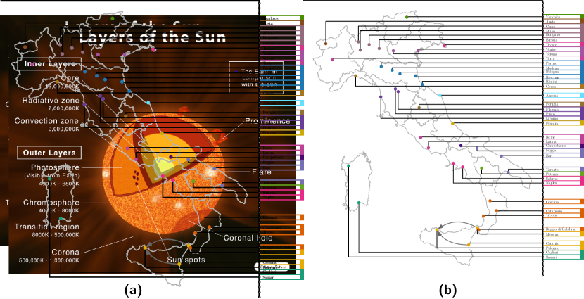
(a) Schematic of the sun. © ScienceFacts.net [8]

(b) Cities in Italy. Labeling with $\mathit{po}$-leaders created by our algorithm described in Section 3.2.

Figure 1: Labelings that adhere to semantic constraints.

More precisely, we study such constrained labelings in the boundary labeling model, which is a well-studied special case of external labelings. Here, the labels must be placed along a rectangular boundary $\mathcal{B}$ around the illustration [4]. Initial work placed the labels on one or two sides of the boundary, usually the left and right sides. For uniform-height labels, efficient algorithms to compute a labeling that minimizes the length of the leaders [4] or more general optimization functions [7] have been proposed. Polynomial-time approaches to compute a labeling with equal-sized labels on (up to) all four sides of the boundary are also known [26]. For non-uniform height labels, (weak) NP-hardness has been shown in the general two-sided [4], and different one-sided settings [3, 14]. Different leader styles have been considered, and we refer to the user study of Barth et al. [1] and the survey of Bekos et al. [5] for an overview. In this paper, we will focus on a frequently used class of L-shaped leaders called $\mathit{po}$-leaders that consist of two segments: one is parallel and the other orthogonal to the side of the boundary on which the label is placed [4], as shown in Figure 1(b). These $\mathit{po}$-leaders turned out as the recommended leader type in the study of Barth et al. [1] as they performed well in various readability tasks and received high user preference ratings.

The literature considered various extensions of boundary labeling [2, 14, 19, 20], and we broaden this body of work with our paper that aims at systematically investigating the above-mentioned constraints in boundary labeling from an algorithmic perspective.

Problem Description.

Let $\mathcal{S}$ be a set of $n$ sites in $\mathbb{R}^{2}$ enclosed in a bounding box $\mathcal{B}$ and in general position, i.e., no two sites share the same $x$- or $y$-coordinate. For each site $s_{i}\in\mathcal{S}$, we have an open rectangle $\ell_{i}$ of height $h(\ell_{i})$ and some width, which we call the label of the site. The rectangles describe the bounding box of the (textual) labels, which are usually a single line of text in a fixed font size. Hence, we often restrict ourselves to uniform-height labels, but neglect their width. The $\mathit{po}$-leader $\lambda_{i}=(s_{i},p_{i})$ is a polyline consisting of (up to) one vertical and one horizontal segment and connects $s_{i}$ with the port $p_{i}$ of $\ell_{i}$, which is the place where $\lambda_{i}$ touches $\ell_{i}$. We define the port for each label $\ell$ to be at half its height. Let $\Lambda$ be the set of all possible leaders. In a $b$-sided boundary labeling $\mathcal{L}\subseteq\Lambda$ we route for each site $s\in\mathcal{S}$ a leader $\lambda$ to a port $p$ on the right ($b=1$) or the right and left ($b=2$) side of $\mathcal{B}$, s.t. we can (in a post-processing step) place the label $\ell$ for $s$ at $p$ and no two labels will overlap.

(a) Length-minimal

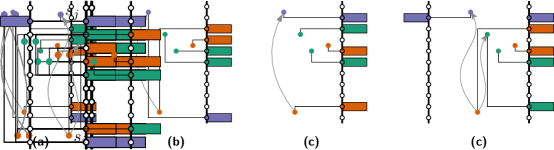
(b) Bend-minimal

(c) A $2$-sided labeling

(d) Non-admissable

Figure 2: Colors indicate grouping and arcs ordering constraints. Labelings that are optimal w.r.t. (2(a)) the total leader length and  (2(b)) the number of bends. In the $2$-sided layout (2(c)) the ordering constraint $s_{i}\preccurlyeq s_{j}$ is not enforced since $\ell_{i}$ and $\ell_{j}$ are on different sides. Note that (2(d)) is a planar but non-admissible length-minimal labeling.

If we are given a finite set of $m$ candidates for the ports $\mathcal{P}$, we say that we have fixed ports, otherwise $\mathcal{P}$ consists of the respective side(s) of $\mathcal{B}$ and is called sliding ports. A labeling is called planar if no two labels overlap and there is no leader-leader or leader-site crossing. We can access the $x$- and $y$-coordinate of a site or port with $x(\cdot)$ and $y(\cdot)$. Furthermore, we are given a set of constraints $\mathcal{C}=\left(\mathscr{G},\preccurlyeq\right)$, consisting of a family of grouping constraints $\mathscr{G}$ and a partial order $\preccurlyeq$ on the sites. A grouping constraint $\emptyset\neq\mathcal{G}\subseteq\mathcal{S}$ enforces that the labels for the sites in $\mathcal{G}$ appear consecutively on the same side of the boundary, as in Figures 2(a), 2(b) and 2(c), but in general there can be gaps between two labels of the same group; compare Figures 2(a) and 2(b). An ordering constraint $s_{i}\preccurlyeq s_{j}$ enforces that we have, for the ports $p_{i}$ and $p_{j}$, $y(p_{i})\geq y(p_{j})$ if they are on the same side of $\mathcal{B}$, i.e., if the labels $\ell_{j}$ and $\ell_{i}$ are placed on the same side of $\mathcal{B}$, then $\ell_{j}$ must not appear above $\ell_{i}$ (see also Figure 2(c)). We assume the existence of reflexive and transitive constraints in $\preccurlyeq$ and denote with $r$ the number of remaining constraints in the transitive reduction of $(\mathcal{S},\preccurlyeq)$. The number of grouping constraints will be denoted with $k$.

We say that a labeling respects the grouping/ordering constraints if all the grouping/ordering constraints are satisfied. Furthermore, we call the grouping/ordering constraints consistent if there exists a (not necessarily planar) labeling that respects them. Similarly, the constraints $\mathcal{C}=\left(\mathscr{G},\preccurlyeq\right)$ are consistent if there exists a (not necessarily planar) labeling that respects $\mathscr{G}$ and $\preccurlyeq$ simultaneously. Finally, a labeling is admissible if it is planar and respects the constraints. Furthermore, if an admissible labeling exists, we aim for one that optimizes a quality criterion expressed by a function $f\colon\Lambda\to\mathbb{R}_{0}^{+}$. In this paper, the optimization function $f$ measures the length of a leader or expresses whether it has a bend or not. Figure 2 highlights the differences and shows in (2(d)) that an optimal admissible labeling might be, w.r.t. the quality criterion expressed by $f$, worse than its planar (but non-admissible) counterpart.

In an instance $\mathcal{I}$ of the Constrained $b$-Sided Boundary Labeling problem ($b$-CBL in short), we ask for an admissible $b$-sided $\mathit{po}$-labeling $\mathcal{L}^{*}$ for $\mathcal{I}$ (possibly on a set of $m$ ports $\mathcal{P}$) that minimizes $\sum_{\lambda\in\mathcal{L}^{*}}f(\lambda)$ or report that no admissible labeling exists.

Related Work on Constrained External Labeling.

Our work is in line with (recent) efforts to integrate semantic constraints into the external labeling model. The survey of Bekos et al. [5] reports a few papers that group labels. Some results consider heuristic label placements in interactive 3D visualizations [21, 22] or group (spatially close) sites together to label them with a single label [13, 29, 35], bundle the leaders [30], or align the labels [36]. These “groupings” are often driven by the distance between (similar) sites and do not allow defining the groups beforehand. To the best of our knowledge, Niedermann et al. [31] are the first that support the explicit grouping of labels while ensuring non-crossing leaders. They proposed a contour labeling algorithm, a generalization of boundary labeling, that can be extended to group sets of labels on the contour as hard constraints in their model. However, they did not analyze this extension in detail and do not support ordering constraints. Recently, Gedicke et al. [18] tried to maximize the number of respected groups that arise from the spatial proximity of the sites or their semantics, i.e., they reward a labeling also based on the number of consecutive labels from the same group. They disallow assigning a site to more than one group, but see combining spatial and semantic groups as an interesting direction for further research. We work towards that goal, as we allow grouping constraints to overlap. Finally, we want to mention the work by Klawitter et al. [28] on visualizing geophylogenies, by embedding a binary (phylogenetic) tree on one side of the boundary. Each leaf of the tree corresponds to a site, and the goal is to connect them using straight-line leaders with few crossings. Such trees implicitly encode grouping constraints, as two sites with a short path between their leaves must be labeled close together on the boundary. In contrast to our work, Klawitter et al. not only considered a different optimization function, but they also restrict themselves to binary trees, which can only represent a limited set of grouping constraints.

Contributions.

Firstly, we show in Section 2 that finding an admissible constrained two-sided boundary labeling is NP-complete, even for uniform-height labels and on fixed ports. Secondly, in Section 3, we take a closer look at 1-CBL. We prove that it is weakly NP-hard to find an admissible labeling with sliding ports and unrestricted label heights. Nevertheless, we also present two polynomial-time algorithms: One for fixed ports and unrestricted label sizes, and one for sliding ports and uniform-height labels. We furthermore implemented the former algorithm and report in Section 4 on an experimental evaluation of its performance.

2 Constrained Two-Sided Boundary Labeling is NP-complete

We will show that finding some admissible two-sided boundary labeling in the presence of grouping and ordering constraints is NP-complete, even if we have uniform-height labels and fixed ports. The crucial ingredient of the reduction is the observation that we can use ordering constraints to transmit information: For the ordering constraint $s\preccurlyeq s^{\prime}$, if the geometric properties of the instance require us to label $s$ below $s^{\prime}$, then any admissible labeling must label $s$ and $s^{\prime}$ on opposite sides of $\mathcal{B}$.

Construction of the Instance.

We reduce from Monotone 1-In-3 Sat, which is a restricted version of 3-Sat, where each clause contains only positive literals, i.e., the variables appear only non-negated, and a clause is satisfied iff exactly one literal evaluates to true [17]. It is known [17, 33] that this problem is NP-complete. For ease of presentation, the following construction will not be in general position. However, we can always perturbate some sites slightly without affecting the correctness of the reduction. Furthermore, note that we will place the ports (and sites) such that there is sufficient vertical space between any two ports and both can be used without overlapping labels. From top to bottom, we will assign a vertical slice on the boundary to each clause, and one for all variables together. All sites and ports placed for a clause are contained within their slice, while all variable related sites and ports are contained in the lowest slice. All slices are pairwise disjoint and separated by blocker gadgets. In a blocker gadget, the placement of the sites together with the grouping constraints indicated in Figure 3 allows only one admissible labeling for them, namely the one shown in Figure 3(b).

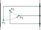
(a) Substructure of the blocker gadget. We add the grouping constraint $\{s_{1},s_{2},s_{3}\}$ and the ordering constraints $s_{1}\preccurlyeq s_{2}$ and $s_{2}\preccurlyeq s_{3}$.

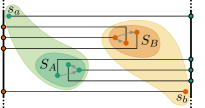
(b) The complete blocker gadget and its only admissible labeling. $S_{A}$ and $S_{B}$ are created as in (3(a)).

Figure 3: The gadget blocker that subdivides the instance.

By placing the sites $s_{a}$ and $s_{b}$ from Figure 3(b) sufficiently close to the boundary, they partition the instance by blocking other leaders from passing through.

For each variable $x_{i}$, we place a site $s_{i}$ and two ports, one on each the left ($p_{i}^{0}$) and one on the right ($p_{i}^{1}$) side of the boundary. Intuitively, if the site is labeled on the right (left), the variable is set to true (false). For each clause $C_{j}$ we place a gadget consisting of three sites, $c_{j}^{1}$, $c_{j}^{2}$, and $c_{j}^{3}$, one for each occurring variable, arranged horizontally, and three ports, one on the left side of the boundary and below the sites, and two on the right side of the boundary and above the sites. For every variable in the clause, we add an ordering constraint, which forces the label of the variable site to be placed above the label of the clause site. Since the blockers prevent any variable site to be labeled above a clause site, only one variable can be labeled on the right boundary (corresponding to its truth value being true). This is the variable, which satisfies the clause. Therefore, by setting exactly those variables whose sites are (in an admissible labeling) labeled to the right to true, we obtain a variable assignment in which exactly one variable per clause is true. Figure 4 gives an overview of the construction by means of a small example.

(a) The constructed instance.

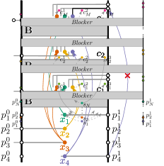
(b) A (non-admissible) labeling that violates an ordering constraint.

Figure 4: The instance created by our reduction for the formula $({x_{1}}\lor x_{2}\lor x_{3})\land(x_{2}\lor{x_{3}}\lor x_{4})\land({x_{1}}\lor{x_{3}}\lor{x_{4}})$. Ordering constraints between variables and their occurrences in clauses are indicated in (4(a)). While we can label the vertices of some clauses such that all constraints are respected, since the formula is a No-instance of Monotone 1-In-3 Sat, at least one ordering constraint has to be violated as highlighted with the black leader in (4(b)).

NP-containment follows readily from the possibility to check admissibility of a labeling in polynomial time.

Theorem 2.1.

Deciding if an instance of 2-CBL has an admissible labeling is NP-complete, even for uniform-height labels and fixed ports.

Proof 2.2.

We argue NP-containment and NP-hardness separately. *NP-containment. Given an instance $\mathcal{I}$ of 2-CBL, we can describe an admissible (witness) labeling $\mathcal{L}$ as a function from the domain of the sites into the co-domain of the ports. Hence, it uses $\mathcal{O}(nm)$ space. To check whether $\mathcal{L}$ is planar, we evaluate all $\mathcal{O}(n^{2})$ leader combinations in $\mathcal{O}(1)$ time each. For the grouping constraints, we check for each of the $k$ groups whether the corresponding $\mathcal{O}(n)$ sites are labeled on the same side of the boundary and no other label is between them. Finally, we can check the $r$ ordering constraints in $\mathcal{O}(r)=\mathcal{O}(n^{2})$ time. Therefore, we can check whether $\mathcal{L}$ is admissible in $\mathcal{O}(n^{2}+kn)$ time. Since these are all polynomials in the input size, NP-containment of 2-CBL follows.

*NP-hardness. We show NP-hardness using the reduction from Monotone 1-In-3 Sat to 2-CBL described in Section 2. Let $\varphi=(\mathcal{X},C)$ be an instance of Monotone 1-In-3 Sat, consisting of $N$ variables $\mathcal{X}=\{x_{1},\ldots,x_{n}\}$ and $M$ clauses $C=\{C_{1},\ldots,C_{M}\}$, and $\mathcal{I}(\varphi)$ the corresponding instance of 2-CBL. Let $\overline{\preccurlyeq}$ be the ordering constraints in $\mathcal{I}(\varphi)$ that put the sites for variables into relation with the sites for the clauses in which they occur. Assuming that each clause gadget is “responsible” for the blocker immediately below it, we derive that we create in total $M$ blocker gadgets. From Figure 3, we can see that each blocker consists of eight sites and eight ports. Each variable gives us one site and two ports, and each clause three sites and three ports. Hence, $\mathcal{I}(\varphi)$ consists of $8M+N+3M=11M+N$ sites and $8M+2N+3M=11M+2N$ ports. Regarding the constraints, we have $4M$ grouping and $4M$ ordering constraints from the blockers. Together with the $3M$ ordering constraints from $\overline{\preccurlyeq}$, three per clause, this sums up to $4M$ grouping and $7M$ ordering constraints. To analyze the height of $\mathcal{I}(\varphi)$ (excluding the height of the labels), we set w.l.o.g. $h=1$. Then, a vertical distance of one between any two neighboring ports on the same side of the boundary is sufficient to maintain correctness of our reduction. For a single blocker gadget, this then corresponds to a height of seven (see Figure 3(b)), which sums up to a height of $7M$ for all blocker gadgets together. Regarding the sites for the variables, we spread them out with a vertical distance of one, the same for the ports. Hence, the variable segment occupies $\left(N-1\right)$ space on the boundary. Finally, for the clause gadgets, we need to ensure that any site can reach the single port on the left side of the boundary. This can be done by placing that port at a distance of one below the sites. On the right side, we can place the two ports a distance of one and two above the three sites. This gives a height of $3M$ for all $M$ clauses together. Summing everything up, we get a height of $7M+N-1+3M+2M=12M+N-1$ for $\mathcal{I}(\varphi)$, excluding the labels, where the last $2M$ follow from the vertical offset we have to maintain before and after each blocker so that they do not interfere with the other building blocks of our reduction. We can assume the width of $\mathcal{I}(\varphi)$ to be constant. Therefore, $\mathcal{I}(\varphi)$ has polynomial size and can be created in polynomial time with respect to the size of $\varphi$. It remains to show the correctness of our reduction.

*($\boldsymbol{\Rightarrow}$) Assume that $\varphi$ is a positive instance of Monotone 1-In-3 Sat. Hence, there exists a truth assignment $\Gamma\colon\mathcal{X}\to\{0,1\}$ s.t. for each clause $C_{i}\in C$, $1\leq i\leq M$, we can find a variable $x_{j}\in C_{i}$ so that $\Gamma(x_{j})=1$ and $\Gamma(x_{j^{\prime}})=0$, for all $x_{j^{\prime}}\in C_{i}$ with $x_{j}\neq x_{j^{\prime}}$, i.e., exactly one literal of each clause evaluates to true under $\Gamma$. We replicate this assignment in a labeling $\mathcal{L}$ of $\mathcal{I}(\varphi)$ by labeling $s_{i}$, $1\leq i\leq N$, at $p_{i}^{1}$ if $\Gamma(x_{i})=1$, otherwise at $p_{i}^{0}$. We label the sites in the clause gadget on the left boundary if the corresponding variable they represent satisfies the clause, i.e., is true, and otherwise on the right side of the boundary. For the sites that make up the blocker gadgets, we label them according to Figure 3(b). What is left to do is argue that $\mathcal{L}$ is admissible. For the sites in the blocker gadgets, this is true by construction. As for any variable $x\in\mathcal{X}$, we have either $\Gamma(x)=1$ or $\Gamma(x)=0$, but never both, the label positions for the sites representing the variables are well-defined. Since we placed the ports and sites with sufficient space from each other, mimicking $\Gamma$ in $\mathcal{L}$ as described above will always result in an admissible labeling. For the sites in the clause gadgets, as $\Gamma$ ensures that exactly one literal evaluates to true, we know that one site will be labeled at the left boundary and the other two at the right boundary. This is exactly the distribution of the three ports we have chosen when creating the clause gadgets (see Figure 4). Furthermore, we have ensured that no matter which two sites we label on the right side, there is a way to label them. Therefore, $\mathcal{L}$ is planar. To show that $\mathcal{L}$ respects also the constraints, we first note that we respect the constraints in the blocker gadgets by construction. Therefore, we only have to consider the ordering constraints from $\overline{\preccurlyeq}$. Let the variable $x_{i}$ appear in the clause $C_{j}$ and let $s_{i}\preccurlyeq c_{j}^{l}$, $l\in\{1,2,3\}$, be the ordering constraint from $\overline{\preccurlyeq}$ that puts them into relation. Since $s_{i}$ represents a variable and $c_{j}^{l}$ its occurrence in a clause, we know that $s_{i}$ will be labeled below $c_{j}^{l}$ in $\mathcal{L}$. Therefore, to respect $s_{i}\preccurlyeq c_{j}^{l}$, we must show that $s_{i}$ and $c_{j}^{l}$ are labeled on different sides of the boundary. There are two cases: $\Gamma(x_{i})=0$ or $\Gamma(x_{i})=1$. In the former case, we label $s_{i}$ on the left side and, as the clause $C_{i}$ is then not satisfied by the variable $x_{i}$, $c_{j}^{l}$ is labeled on the right side. In the latter case, i.e., if $\Gamma(x_{i})=1$, we label $s_{i}$ on the right side and, as it satisfies the clause, $c_{j}^{l}$ is (the only site in this clause gadget that is) labeled on the left side. As we label them in both cases on different sides of the boundary, this ordering constraint is trivially satisfied. Since we selected $s_{i}\preccurlyeq c_{j}^{l}$ arbitrarily, we know that this holds for all constraints in $\overline{\preccurlyeq}$. Hence, $\mathcal{L}$ is admissible.

*($\boldsymbol{\Leftarrow}$) Let $\mathcal{I}(\varphi)$ possess an admissible labeling $\mathcal{L}$. Based on $\mathcal{L}$, we create a truth assignment $\Gamma\colon\mathcal{X}\to\{0,1\}$ over $\mathcal{X}$ with $\Gamma(x_{i})=1$ if $\mathcal{L}$ labels $s_{i}$ at $p_{i}^{1}$, $1\leq i\leq N$. Otherwise, i.e., if $\mathcal{L}$ labels $s_{i}$ at $p_{i}^{0}$, we set $\Gamma(x_{i})=0$. Due to the structure of the variable block, we can assume that we label each $s_{i}$ at one of those two ports, and thus is $\Gamma$ well-defined. All that remains to do is to show that in every clause $C_{i}$ exactly one literal evaluates to true. We remind the reader that every literal in $\varphi$ is an un-negated variable. $\mathcal{L}$ respects all the constraints of $\mathcal{I}(\varphi)$, in particular the ordering constraints $\overline{\preccurlyeq}$. However, observe that due to the blocker gadgets, especially the one between the variable slice and the first clause gadget, in any admissible labeling, and therefore also in $\mathcal{L}$, all sites in the variable slice are labeled below those in the clause gadgets. Therefore, to respect the constraints in $\overline{\preccurlyeq}$, $\mathcal{L}$ must satisfy them “trivially”, i.e., by labeling the sites on different sides of the boundary. Hence, for each site $s_{i}$ in the variable slice that we label on the right side, i.e., at $p_{i}^{1}$, we must label all sites for its occurrences in clauses on the left side, as there is a corresponding constraint in $\overline{\preccurlyeq}$. A symmetric argument holds if we label $s_{i}$ on the left side. However, since for every clause gadget representing some clause $C_{j}$, $1\leq j\leq M$, we create three ordering constraints in $\overline{\preccurlyeq}$ and there is only one port on the left side and two ports on the right side, we know that $\mathcal{L}$ can only be admissible if exactly one of the three sites that make up the clause gadget is labeled on the left side, i.e., considered true. Consequently, $\Gamma$ satisfies exactly one literal of each clause in $\varphi$, i.e., $\varphi$ is a positive instance of Monotone 1-In-3 Sat.

3 The Constrained One-Sided Boundary Labeling Problem

In the light of Theorem 2.1, the natural next step is to consider 1-CBL. In Section 3.1, we show that finding an admissible labeling for an instance of 1-CBL is weakly NP-hard. However, by restricting the input to either fixed ports (Section 3.2) or uniform labels (Section 3.3), we can obtain polynomial-time algorithms. Observe that this is in hard contrast to 2-CBL, where we have shown that the problem is NP-complete even for a uniform label size and fixed ports.

3.1 Constrained One-Sided Boundary Labeling is Weakly NP-hard

To show that it is weakly NP-hard to find an admissible labeling in an instance of 1-CBL, we can adapt the idea of Fink and Suri [14]. They reduce Partition to the problem of finding a planar labeling with non-uniform height labels and sliding ports in the presence of a single obstacle on the plane. We create with our constraints an obstacle on the boundary that serves the same purpose. The following illustration is not in general position and contains leader-site crossings. As before, this can be resolved by perturbating some sites slightly.

Construction of the Instance.

We will first give a reduction that only uses grouping constraints. In the end, we show how we can replace the grouping constraints by ordering constraints. Let $\left(\mathcal{A}=\{a_{1},\ldots a_{N}\},w\colon\mathcal{A}\to\mathbb{N}\right)$ be an instance of Partition with $\sum_{a\in\mathcal{A}}w(a)=2A$, for some $A\in\mathbb{N}$ [17]. We create for each element $a_{i}$ a site $s_{i}$ whose corresponding label has a height of $w(a_{i})$, and place the sites on a horizontal line next to each other. Furthermore, we create five sites, $b_{1}$ to $b_{5}$, with corresponding labels of height 1 for $b_{1}$ and $b_{5}$, height $\lfloor\frac{A-4}{2}\rfloor$ for $b_{2}$ and $b_{4}$, and height 2 or 3 for $b_{3}$, depending on whether $A$ is even or odd, respectively, and place them as in Figure 5. Observe that the height of the labels for $b_{1}$ to $b_{5}$ sums up to $A$. We create the grouping constraints $\{\{b_{1},b_{2},b_{3},b_{4},b_{5}\},\{b_{1},b_{2},b_{3}\},\{b_{3},b_{4},b_{5}\},\{b_{2},b_{3},b_{4}\},\{b_{1},b_{2}\},\{b_{4},b_{5}\}\}$.

Figure 5: Creating an obstacle using grouping constraints as indicated by colored bands. An alternative way of forcing the same structure with only ordering constraints is shown with the arrows.

These grouping constraints enforce that any admissible labeling must label these sites as indicated in Figure 5. Since there is neither an alternative order of the labels nor room to slide around, the labels of these sites must be placed contiguously, without any free space, and at that fixed position on the boundary. Hence, we call the resulting structure a block. We create two similar blocks above and below the sites for $\mathcal{A}$ and leave between them a space of $A$ on the boundary, respectively. We visualize this construction in Figure 6 and observe that this creates two $A$-high free windows on the boundary where we can place the labels for the sites representing the elements of $\mathcal{A}$ in. Finally, note that the grouping constraints we used to keep the labels for the sites of the blocks in place can be exchanged by the ordering constraints $\{b_{1}\preccurlyeq b_{2},b_{2}\preccurlyeq b_{3},b_{3}\preccurlyeq b_{4},b_{4}\preccurlyeq b_{5}\}$ (also shown in Figure 5). Similar substitutions have to be performed in the other two blocks. As this exchanges 18 grouping constraints with twelve ordering constraints, we obtain Theorem 3.1.

Theorem 3.1.

Deciding if an instance of 1-CBL has an admissible labeling is weakly NP-hard, even for a constant number of grouping or ordering constraints.

Proof 3.2.

For an instance $(\mathcal{A},\omega)$ of Partition, let $\mathcal{I}(\mathcal{A},\omega)$ be the created instance for 1-CBL according to our reduction from Section 3.1. See Figure 6 for an illustration of the created instance. Note that we use in Figure 6 the sites $x_{1}$ to $x_{5}$, $b_{1}$ to $b_{5}$, and $y_{1}$ to $y_{5}$ to create the blocker above, next to, and below the sites for $\mathcal{A}$, respectively. Regarding the size of the created instance, we note that $\mathcal{I}(\mathcal{A},\omega)$ has $N+15$ sites and $18$ grouping ($12$ ordering) constraints, where $N=\left|\mathcal{A}\right|$. Furthermore, the height is linear in $A$, where we defined $2A=\sum_{a\in\mathcal{A}}w(a)$. For the correctness of the reduction, we observe the following.

*($\boldsymbol{\Rightarrow}$) Let $\left(\mathcal{A},w\right)$ be a positive instance of Partition and $\mathcal{A}_{1}$ and $\mathcal{A}_{2}$ a corresponding solution, i.e., we have $\sum_{a\in\mathcal{A}_{1}}w(a)=\sum_{a\in\mathcal{A}_{2}}w(a)=A$. We transform this information now into an admissible labeling for $\mathcal{I}(\mathcal{A},w)$. The blocks are labeled as in Figures 5 and 6. To determine the position of the labels for the remaining sites, $s_{1}$ to $s_{N}$, we traverse them from left to right. For any site $s_{i}$, $1\leq i\leq N$, we check whether its corresponding element $a_{i}$ is in $\mathcal{A}_{1}$ or $\mathcal{A}_{2}$. If it is in $\mathcal{A}_{1}$, we place the label for $s_{i}$ as far up as possible, i.e., inside the upper free space of Figure 6. On the other hand, if it is in $\mathcal{A}_{2}$, we place the label for $s_{i}$ as far down as possible, i.e., inside the lower free space of Figure 6. As the sum of the weights of the elements of $\mathcal{A}_{1}$ and $\mathcal{A}_{2}$ evaluates to $A$, respectively, and we reflect the values of the sum in the height of the respective labels, it is guaranteed that we can place all labels for sites that represent entries in $\mathcal{A}_{1}$ and $\mathcal{A}_{2}$ in the respective $A$-high windows. Finally, by traversing the sites from left to right and assigning the outermost possible position for the respective label, we guarantee that the resulting labeling is planar and thus admissible.

*($\boldsymbol{\Leftarrow}$) Let $\mathcal{L}$ be an admissible labeling for $\mathcal{I}(\mathcal{A},w)$. By the placement of the sites for the elements in $\mathcal{A}$ and the (sites for the) blocks, which is shown in Figure 6, we conclude that the labels for the sites $s_{1}$ to $s_{N}$ can only be inside the $A$-high windows on the boundary. We define $\mathcal{A}_{1}$ as the set of elements whose corresponding site is labeled between $x_{5}$ and $b_{1}$ and $\mathcal{A}_{2}$ as the one where the label is between $b_{5}$ and $y_{1}$. Recall that in each of these windows, there is only space for that many sites such that the sum of their label heights equals $A$. Therefore, we know that $A=\sum_{a\in\mathcal{A}_{1}}w(a)=\sum_{a\in\mathcal{A}_{2}}w(a)$ must hold, i.e., $\left(\mathcal{A},w\right)$ is a positive instance of Partition.

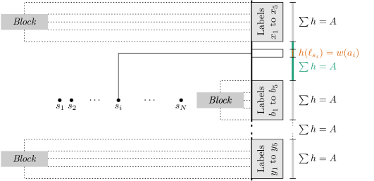
Figure 6: The placement of the sites in the reduction that shows weakly NP-hardness for 1-CBL. Gray boxes visualize the blocks.

3.2 Fixed Ports

We assume that we are given a set $\mathcal{P}$ of $m\geq n$ ports. Benkert et al. [7] observed that in a planar labeling $\mathcal{L}$, the leader $\lambda_{L}$ connecting the leftmost site $s_{L}\in\mathcal{S}$ with some port $p_{L}$ splits the instance $\mathcal{I}$ into two independent sub-instances, $\mathcal{I}_{1}$ and $\mathcal{I}_{2}$, excluding $s_{L}$ and $p_{L}$. Therefore, we can describe a sub-instance $I$ of $\mathcal{I}$ by two leaders $(s_{1},p_{1})$ and $(s_{2},p_{2})$ that bound the sub-instance from above and below, respectively. We denote the sub-instance as $I=(s_{1},p_{1},s_{2},p_{2})$ and refer with ${\mathcal{S}}(I)$ (${\mathcal{P}}(I)$) to the sites (ports) in $I$, excluding those used in the definition of $I$, i.e., ${\mathcal{S}}(I)\coloneqq\{s\in\mathcal{S}\mid x(s_{1})<x(s),\ x(s_{2})<x(s),\ y(p_{1})<y(s)<y(p_{2})\}$ and ${\mathcal{P}}(I)\coloneqq\{p\in\mathcal{P}\mid y(p_{1})<y(p)<y(p_{2})\}$. Similarly, for a leader $\lambda=(s,p)$, we say that a site $s^{\prime}$ with $x(s)<x(s^{\prime})$ is above $\lambda$ if $y(s^{\prime})>y(p)$ holds and below $\lambda$ if $y(s^{\prime})<y(p)$ holds. See also Figure 7 for a visualization of these definitions.

Two more observations about admissible labelings can be made: First, $\lambda_{L}$ can never split sites $s,s^{\prime}\in\mathcal{G}$ with $s_{L}\notin\mathcal{G}$. Second, $\lambda_{L}$ never splits sites $s,s^{\prime}\in\mathcal{S}$ with $s$ above $\lambda_{L}$ and $s^{\prime}$ below $\lambda_{L}$, for which we have $s^{\prime}\preccurlyeq s_{L}$, $s^{\prime}\preccurlyeq s$, or $s_{L}\preccurlyeq s$. Now, we could immediately define a dynamic programming (DP) algorithm that evaluates the induced sub-instances for each leader that adheres to these observations. However, we would then check every constraint in each sub-instance and not make use of implicit constraints given by, for example, overlapping groups. The following data structure makes these implicit constraints explicit.

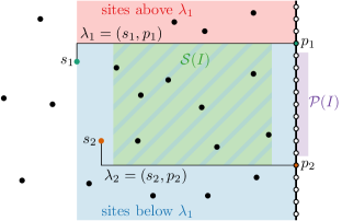
Figure 7: A sub-instance $I=(s_{1},p_{1},s_{2},p_{2})$ of our DP-algorithm and the used notation.

PQ-A-Graphs.

Every labeling $\mathcal{L}$ induces a permutation $\pi$ of the sites by reading the labels from top to bottom. Assume $k>0$ and let $M(\mathcal{S},\mathscr{G})$ be a $n\times k$ binary matrix with $m_{i,j}=1$ iff $s_{i}\in\mathcal{G}_{j}$ for $\mathcal{G}_{j}\in\mathscr{G}$. We call $M(\mathcal{S},\mathscr{G})$ the sites vs. groups matrix, and observe that $\mathcal{L}$ satisfies the constraint $\mathcal{G}_{j}$ iff the ones in the column $j$ of $M(\mathcal{S},\mathscr{G})$ are consecutive after we order the rows of $M(\mathcal{S},\mathscr{G})$ according to $\pi$. If this holds for all columns of $M(\mathcal{S},\mathscr{G})$, then the matrix has the so-called consecutive ones property (C1P) [16].

Lemma 3.3.

$\mathscr{G}$ are consistent for $\mathcal{S}$ iff $M(\mathcal{S},\mathscr{G})$ has the C1P.

Proof 3.4.

We show both directions separately. For ease of presentation, we assume $m=n$ fixed ports on the boundary. However, the proof extends readily to $m\geq n$ or sliding ports.

*($\boldsymbol{\Rightarrow}$) We assume that the grouping constraints $\mathscr{G}$ are consistent. Let $\mathcal{L}$ be a (not necessarily planar) labeling that respects all grouping constraints. We order the rows of $M(\mathcal{S},\mathscr{G})$ according to the order imposed by $\mathcal{L}$ on the sites $\mathcal{S}$, i.e., when reading the labels top-to-bottom, and obtain thus a permutation $\pi$ of $\mathcal{S}$. As $\mathcal{L}$ is a witness labeling for the consistency of $\mathscr{G}$, each group $\mathcal{G}_{j}\in\mathscr{G}$, $1\leq j\leq k$, is not intersected by a label for a site that is not part of $\mathcal{G}_{j}$. Therefore, for each group $\mathcal{G}_{j}$, the ones in the $j$th column of $M(\mathcal{S},\mathscr{G})$ must be consecutive. Consequently, $\pi$ witnesses that $M(\mathcal{S},\mathscr{G})$ has the C1P.

*($\boldsymbol{\Leftarrow}$) We assume that $M(\mathcal{S},\mathscr{G})$ has the C1P. This means there exists a permutation $\pi$ of the rows, i.e., the sites, such that the ones in each column, i.e., for each group, are consecutive. If we order the labels according to the order of their respective sites in $\pi$ and create the corresponding (not necessarily planar) labeling $\mathcal{L}$, which is uniquely defined on the $m=n$ ports, $\mathcal{L}$ will respect all the grouping constraints. If not, this would mean that we have a group $\mathcal{G}_{j}\in\mathscr{G}$, $1\leq j\leq k$, that is intersected by a label for a site $s_{i}\notin\mathcal{G}_{j}$ outside the group. However, by our definition of $M(\mathcal{S},\mathscr{G})$, $m_{i,j}=0$ must hold, and since the group $\mathcal{G}_{j}$ is intersected by $s_{i}$, we know that $m_{i_{1},j}=m_{i_{2},j}=1$ holds, for some $\pi(i_{1})<\pi(i)<\pi(i_{2})$, $1\leq i,i_{1},i_{2}\leq n$. This would mean that $\pi$ is not a witness for $M(\mathcal{S},\mathscr{G})$ having the C1P, contradicting our initial assumption. Therefore, $\mathcal{L}$ must witness the consistency of $\mathscr{G}$.

Booth and Lueker [9] propose an algorithm to check whether a binary matrix has the C1P. They use a PQ-Tree to keep track of the allowed row permutations. A PQ-Tree $\tau$, for a given set $\mathcal{A}$ of elements, is a rooted tree with one leaf for each element of a $\mathcal{A}$ and two different types of internal nodes $t$: P-nodes, that allow to freely permute the children of $t$, and Q-nodes, where the children of $t$ can only be inversed [9]. Lemma 3.3 tells us that each family of consistent grouping constraints can be represented by a PQ-Tree. Furthermore, we can interpret each subtree of the PQ-Tree as a grouping constraint and call them the canonical groups. However, not every grouping constraint results in a canonical group.

While we can deduce from Lemma 3.3 that PQ-Trees can represent families of consistent grouping constraints, it is folklore that directed graphs can be used to represent partial orders, i.e., our ordering constraints. We now combine these two data structures into PQ-A-Graphs.

Definition 3.5 (PQ-A-Graph).

Let $\mathcal{S}$ be a set of sites, $\mathscr{G}$ be a family of consistent grouping constraints, and $\preccurlyeq$ be a partial order on $\mathcal{S}$. The PQ-A-Graph $\mathcal{T}=(\tau{},A)$ consists of the PQ-Tree $\tau$ for $\mathscr{G}$, on whose leaves we embed the arcs $A$ of a directed graph representing $\preccurlyeq$.

We denote with $T_{i}$ the subtree in the underlying PQ-Tree $\tau$ rooted at the node $t_{i}$ and with $\text{leaves}(T_{i})$ the leaf set. Figure 8 visualizes a PQ-A-Graph and the introduced terminology. Furthermore, observe that checking on the consistency of $\mathcal{C}=\left(\mathscr{G},\preccurlyeq\right)$ is equivalent to solving the Reorder problem on $\tau$ and $\preccurlyeq$, i.e., asking whether we can re-order $\text{leaves}(\tau{})$ such that the order induced by reading them from left to right extends the partial order $\preccurlyeq$ [27].

Lemma 3.6.

We can check if the constraints $\mathcal{C}=\left(\mathscr{G},\preccurlyeq\right)$ are consistent for $\mathcal{S}$ and, if so, create the PQ-A-Graph $\mathcal{T}$ in $\mathcal{O}(n+k+r+\sum_{\mathcal{G}\in\mathscr{G}}\left|\mathcal{G}\right|)$ time. $\mathcal{T}$ uses $\mathcal{O}(n+r)$ space.

Proof 3.7.

We prove the statements of the lemma individually.

*Checking the Consistency of $\boldsymbol{\mathscr{G}}$. We showed in Lemma 3.3 that $\mathscr{G}$ being consistent for $\mathcal{S}$ is equivalent to the sites vs. groups matrix $M(\mathcal{S},\mathscr{G})$ having the C1P. Booth and Lueker [9] propose an algorithm to check whether a binary matrix $M$ has the C1P. Since their algorithm decomposes $M$ into its columns to build a PQ-Tree $\tau$ out of those, which for $M(\mathcal{S},\mathscr{G})$ would correspond to the groups $\mathcal{G}\in\mathscr{G}$, we do not need to compute $M(\mathcal{S},\mathscr{G})$ but can directly work with $\mathscr{G}$. Plugging in the resulting equivalences, we derive that their algorithm runs in $\mathcal{O}(n+k+\sum_{\mathcal{G}\in\mathscr{G}}\left|\mathcal{G}\right|)$ time [9, Theorem 6]. If it outputs that $M(\mathcal{S},\mathscr{G})$ does not have the C1P, then we know that $\mathcal{C}$ cannot be consistent for $\mathcal{S}$. On the other hand, if it outputs that $M(\mathcal{S},\mathscr{G})$ has the C1P, we can modify the algorithm to also return the computed PQ-Tree $\tau$ without spending additional time.

*Checking the Consistency of $\boldsymbol{\preccurlyeq}$. It remains to check whether $\tau$ allows for a permutation that extends the partial order $\preccurlyeq$ on the sites. This is equivalent to the instance $(\tau{},\preccurlyeq)$ of the Reorder problem. Klávic et al. show that we can solve this problem in $\mathcal{O}(n+r)$ time [27].

The claimed running time for checking the consistency of $\mathcal{C}=\left(\mathscr{G},\preccurlyeq\right)$ for $\mathcal{S}$ follows then readily. For the rest of the proof, we assume that the constraints $\mathcal{C}$ are consistent for $\mathcal{S}$, as otherwise the corresponding PQ-A-Graph $\mathcal{T}$ might not be defined.

*Creation Time of $\boldsymbol{\mathcal{T}}$. We have already concluded that we can obtain the PQ-Tree $\tau$ in $\mathcal{O}(n+k+\sum_{\mathcal{G}\in\mathscr{G}}\left|\mathcal{G}\right|)$ time using the algorithm by Booth and Lueker [9]. In the following, we assume that we maintain a map that returns for each site $s\in\mathcal{S}$ the corresponding leaf in $\tau$. Since we never add or remove a leaf, maintaining this list does not increase the asymptotic running time of creating the PQ-Tree $\tau$. To finish the creation of $\mathcal{T}$, we have to enrich $\tau$ by the ordering constraints $\preccurlyeq$. Let $s\preccurlyeq s^{\prime}$ be one of those constraints. Since we can find the leaves for $s$ and $s^{\prime}$ in $\tau$ in constant time using our lookup table, adding the corresponding arc to $\tau$ takes $\mathcal{O}(1)$ time. This sums up to $\mathcal{O}(r)$ and together with above arguments we get $\mathcal{O}(n+k+r+\sum_{\mathcal{G}\in\mathscr{G}}\left|\mathcal{G}\right|)$.

*Space Consumption of $\boldsymbol{\mathcal{T}}$. Regarding the space consumption of the underlying PQ-Tree $\tau$, we first note that Booth and Lueker assumed that they work with proper PQ-Trees. This means that any P-node has at least two and any Q-node at least three children, respectively, i.e., there are no (chains of) nodes with a single child [9]. Hence, $\tau$ uses $\mathcal{O}(n)$ space [25]. To embed the arcs on the leaves of $\tau$, we can use adjacency sets, i.e., adjacency lists where we use sets to store the neighbors of the nodes. This gives us constant time look-up while needing $\mathcal{O}(n+r)$ space, and combined with the space consumption of $\tau$, we get $\mathcal{O}(n+r)$.

The Dynamic Programming Algorithm.

Let $I=(s_{1},p_{1},s_{2},p_{2})$ be a sub-instance and $s_{L}$ the leftmost site in $\mathcal{S}$(I). Let $\mathcal{T}(s_{1},s_{2})$ denote the sub-graph of the PQ-A-Graph $\mathcal{T}$ rooted at the lowest common ancestor of $s_{1}$ and $s_{2}$ (in $\mathcal{T}$). Note that $\mathcal{T}(s_{1},s_{2})$ contains all the sites in ${\mathcal{S}}(I)$, together with $s_{1}$ and $s_{2}$, and hence represents all constraints relevant for the sub-instance $I$. Other constraints either do not affect sites in $I$ or are trivially satisfied. Imagine we want to place the label $\ell_{L}$ for $s_{L}$ at the port $p_{L}\in{\mathcal{P}}(I)$. We have to ensure that $\lambda_{L}=(s_{L},p_{L})$ does not violate planarity w.r.t. the already fixed labeling and that in the resulting sub-instances there are enough ports for the sites. Let ${\textsc{Admissible}}(I,\mathcal{T},p_{L})$ be a procedure that checks the following criteria.

1. The label $\ell_{L}$ does not overlap with the labels $\ell_{1}$, placed at $p_{1}$, and $\ell_{2}$, placed at $p_{2}$, for the sites $s_{1}$ and $s_{2}$, respectively, that define the sub-instance $I$.

2. The leader $\lambda_{L}$ does not intersect with a site $s^{\prime}\in{\mathcal{S}}(I)$, $s^{\prime}\neq s_{L}$.

3. In both resulting sub-instances $I_{1}=(s_{1},p_{1},s,p)$ and $I_{2}=(s,p,s_{2},p_{2})$, there are enough ports for all sites, i.e., $\left|{\mathcal{S}}(I_{i})\right|\leq\left|{\mathcal{P}}(I_{i})\right|$, for $i=1,2$.

4. $p_{L}$ respects the constraints expressed by $\mathcal{T}(s_{1},s_{2})$.

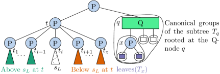
Figure 8: A sample PQ-A-Graph together with the used terminology.

To check the last criterion efficiently, we make use of ${\textsc{RespectsConstraints}}(I,\mathcal{T},\lambda_{L})$, a procedure which we define now. Let $t_{L}$ be the leaf for $s_{L}$ in $\mathcal{T}(s_{1},s_{2})$. There is a unique path from $t_{L}$ to $t_{r}$, which is the root of $\mathcal{T}(s_{1},s_{2})$, which we traverse bottom up and consider each internal node on it. Let $t$ be such a node with the children $t_{1},\dots,t_{z}$ in this order from left to right. Let $T_{i}$, $1\leq i\leq z$, be the subtree that contains the site $s_{L}$, rooted at $t_{i}$. The labels for all sites represented by $\text{leaves}(T_{1}),\dots,\text{leaves}(T_{i-1})$ will be placed above $\ell_{L}$ in any labeling $\mathcal{L}$ of $\mathcal{S}$ in which the children of $t$ are ordered as stated. Therefore, we call these sites above $s_{L}$ (at $t$). Analogously, the sites represented by $\text{leaves}(T_{i+1}),\dots,\text{leaves}(T_{z})$ are below $s_{L}$ (at $t$). Figure 8 visualizes this. The sites represented by $\text{leaves}(T_{i})$ are neither above nor below $s_{L}$ at $t$. It is important to note that we use two different notions of above/below. On the one hand, sites can be above a node $t$ in the PQ-A-Graph $\mathcal{T}(s_{1},s_{2})$, which depends on the order of the children of $t$. On the other hand, a site can also be above a leader $\lambda$, which depends on the (geometric) position of $\lambda$ and is independent of $\mathcal{T}(s_{1},s_{2})$. Recall (and compare) Figure 8 with Figure 7 for the former and latter notion of above and below, respectively.

If $t$ is a P-node, we seek a permutation $\pi$ of the children $t_{1},\dots,t_{z}$ of $t$ in which all the sites in $\mathcal{S}$(I) above $s_{L}$ at $t$ (in the permutation $\pi$) are above $\lambda_{L}$, and all the sites in $\mathcal{S}$(I) below $s_{L}$ at $t$ (in the permutation $\pi$) are below $\lambda_{L}$. This means that it cannot be the case that some sites of the same subtree $T$, where $T$ does not contain $s_{L}$, are above $\lambda_{L}$, while others are below $\lambda_{L}$, as this would imply that we violate the canonical grouping constraint induced by $T$. To not iterate through all possible permutations, we distribute the children of $t$, except $t_{i}$, into two sets, $t_{\text{above}}$ and $t_{\text{below}}$, depending on whether they contain only leaves for sites that should be above or below $s$ at $t$. Depending on the position of $t$ in $\mathcal{T}(s_{1},s_{2})$, the children of $t$ might contain sites that are not part of the instance $I$. In particular, this can be the case when $t$ is an internal node on the path from, for example, $s_{1}$ to $t_{r}$. Unless specified otherwise, whenever we mention in the following the site $s_{1}$, then the same applies to $s_{2}$, but possibly after exchanging above with below.

If $T_{j}$, rooted at a child $t_{j}$ of $t_{i}$, $1\leq j\leq z$, $i\neq j$, only contains sites from ${\mathcal{S}}(I)$, we check whether all the sites are above $\lambda_{L}$, or if all are below $\lambda_{L}$. In the former case, we put $t_{j}$ in the set $t_{\text{above}}$, and in the latter case in $t_{\text{below}}$. Recall that if neither of these cases applies, we know that $\lambda_{L}$ would split a (canonical) group to which $s_{L}$ does not belong, and hence, $p_{L}$ does not respect the constraints at $t$ for $s_{L}$, and we can return with failure.

Otherwise, if $T_{j}$ contains only sites outside the sub-instance and not $s_{1}$, we immediately put it in $t_{\text{above}}$. If $T_{j}$ contains $s_{1}\in\text{leaves}(T_{j})$, it can contain some sites in $I$ and others outside $I$. In this case, we only check whether all sites in $\text{leaves}(T_{j})\cap{\mathcal{S}}(I)$, are above $\lambda_{L}$. For both cases, the definition of $I$ enforce this, as these sites are outside the sub-instance and must, therefore, be above $s_{L}$ at $t$ as $s_{1}$ is also above $s_{L}$ at $t$. Hence, we can return with failure if these checks do not succeed. Furthermore, if $s_{1}\in\text{leaves}(T_{i})$ holds, then $t_{\text{above}}$ must not contain a child $t_{j}$ containing sites from ${\mathcal{S}}(I)$, as they would then be labeled outside $I$, violating the definition of $I$. Figure 9 visualizes this.

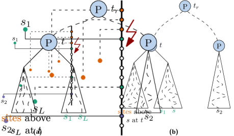
(a) A PQ-A-Graph $\mathcal{T}(s_{1},s_{2})$, rooted at $t_{r}$, with $s_{1}\in\text{leaves}(T_{i})$.

(b) A (sub-)instance $I$, where a wrong permutation of the children of $t$ in $\mathcal{T}(s_{1},s_{2})$ from (9(a)) would label the orange sites outside $I$.

Figure 9: In this situation $t_{\text{above}}$ must not contain subtrees with sites from the sub-instance.

Observe that, as long as $t\neq t_{r}$ holds, we have that $s_{1}$, $s_{2}$, or neither of them is in the subtree rooted at $t$. Hence, the definition of $I$ already dictates whether a child $t_{j}$ of $t$ that contains sites outside the sub-instance must be in $t_{\text{above}}$ or $t_{\text{below}}$. However, if $t=t_{r}$ holds, we must be more careful, as $s_{1}$ and $s_{2}$ are part of the subtree rooted at $t$. Hence, sites outside the sub-instance could be above or below $s_{L}$ at $t$. If a $T_{j}$ does not contain the sites $s_{1}$ and $s_{2}$, and only sites outside $I$, then $t_{j}$ could be put in $t_{\text{above}}$ or $t_{\text{below}}$, unless there is a relevant constraint that allows us to infer the set in which we have to put $t_{j}$. But if there is such a constraint, then it must have been considered the latest when we placed $s_{1}$ or $s_{2}$, as their leaders divided the sites in ${\mathcal{S}}(I)$ from those in $T_{j}$. Hence, it is safe to ignore this child, and we put it in neither of the sets. Similar to before, if $s_{1}\in\text{leaves}(T_{i})$ holds, then $t_{\text{above}}$ must not contain a $t_{j}$ having sites from $I$ and analogous with $t_{\text{below}}$ if we have $s_{2}\in\text{leaves}(T_{i})$.

Observe that we query the position of each site $s^{\prime}$ in a subtree $T_{j}$, $1\leq j\leq z$, $i\neq j$, $\mathcal{O}(1)$ times and determine each time its position w.r.t. the leader $\lambda_{L}$, which takes $\mathcal{O}(1)$ time, or check whether it is in the sub-instance, which also takes $\mathcal{O}(1)$ time. Afterwards, we do not consider this site anymore. Hence, this process can be implemented in $\mathcal{O}(\left|T_{j}\right|)=\mathcal{O}(n)$ time. What remains to do is to ensure the following. There cannot be a site $s_{u}$, represented by a leaf $l_{u}\in\bigcup_{t_{u}\in t_{\text{above}}}\text{leaves}(T_{u})$, a site $s_{v}$, represented by a leaf $l_{v}\in\text{leaves}(T_{i})$, and a site $s_{w}$, represented by a leaf $l_{w}\in\bigcup_{t_{w}\in t_{\text{below}}}\text{leaves}(T_{w})$, such that we have one of the arcs $(s_{v},s_{u})$, $(s_{w},s_{u})$, or $(s_{w},s_{v})$ in $\mathcal{T}(s_{1},s_{2})$. If there are such sites, we know that we violate an ordering constraint and return with failure. To perform these checks efficiently, we can maintain, while computing $t_{\text{above}}$ and $t_{\text{below}}$, a look-up table that stores for each site whether it belongs to $t_{\text{above}}$, $t_{\text{below}}$, or $T_{i}$. Then we check for each of the arcs in $\mathcal{T}(s_{1},s_{2})$ in constant time, whether we violate it or not. Since there are at most $r$ arcs, we can implement these checks to run in $\mathcal{O}(n+r)$ time, which already includes the time required to compute the look-up tables.

The checks that have to be performed if $t$ is a Q-node are conceptually the same, but simpler, since Q-nodes only allow to inverse the order: Either all sites above $s_{L}$ at $t$ are above $\lambda_{L}$, and all sites below $s_{L}$ at $t$ are below $\lambda_{L}$. Or all sites above $s_{L}$ at $t$ are below $\lambda_{L}$, and all sites below $s_{L}$ at $t$ are above $\lambda_{L}$. In the former case, we keep the order of the children at the node $t$ as they are. In the latter case, we inverse the order of the children at the node $t$. Furthermore, there must not be an arc $(s_{u},s_{v})\in\mathcal{T}(s_{1},s_{2})$, $1\leq u,v\leq n$, that prevents this (inversion of the) ordering. Note that if a child of $t$ contains sites outside the sub-instance $I$ but in $\mathcal{T}(s_{1},s_{2})$, one of the two allowed inversions is enforced by the definition of $I$. The above sketched checks for a Q-node trivially run in $\mathcal{O}(n+r)$ time.

Next, we want to argue why we only have to check the subtree of the PQ-A-Graph rooted at the least common ancestor of $s_{1}$ and $s_{2}$, where $s_{1}$ and $s_{2}$ define the sub-instance $I=(s_{1},p_{1},s_{2},p_{2})$. This is because we will respect any constraint that originates from a node $t$ further up in the tree: All sites from $\mathcal{S}$(I) are then in the subtree of the same child of $t$. Let $I^{\prime}=(s_{1}^{\prime},p_{1}^{\prime},s_{2}^{\prime},p_{2}^{\prime})$ be a sub-instance that contains $I$, i.e., we have $s_{1},s_{2}\in{\mathcal{S}}(I^{\prime})$ and $p_{1},p_{2}\in{\mathcal{P}}(I^{\prime})$. Observe that the sub-graph $\mathcal{T}(s_{1}^{\prime},s_{2}^{\prime})$ of $\mathcal{T}$ that we considered for the sub-instance $I^{\prime}$ has its root $t_{r^{\prime}}$ at $t_{r}$ or above $t_{r}$, i.e., $t_{r^{\prime}}=t_{r}$ or $t_{r^{\prime}}$ is an ancestor of $t_{r}$. Thus, on the way from the leftmost site in $I^{\prime}$ to $t_{r^{\prime}}$, we “passed by” $t_{r}$, either directly as $t_{r}$ was a node on the path to $t_{r^{\prime}}$, or indirectly, as $t_{r}$ was a node in a subtree whose leaves we considered. In either case, we ensured that we can respect the constraints there.

Finally, we say that the (candidate) port $p_{L}$ respects the constraints for $s_{L}$ imposed by $\mathcal{T}(s_{1},s_{2})$ in the sub-instance $I=(s_{1},p_{1},s_{2},p_{2})$ if it respects them for $s_{L}$ at every node $t$ on the path from $s_{L}$ to the root of $\mathcal{T}(s_{1},s_{2})$. The procedure ${\textsc{RespectsConstraints}}(I,\mathcal{T},\lambda_{L})$ as defined above performs these checks for each of the $\mathcal{O}(n)$ nodes on the path from $s_{L}$ to $t_{r}$. The following lemma shows that ${\textsc{RespectsConstraints}}(I,\mathcal{T},\lambda_{L})$ runs in $\mathcal{O}(n\left(n+r\right))$ time and uses this to show that ${\textsc{Admissible}}(I,\mathcal{T},p_{L})$ takes $\mathcal{O}(n^{2}+nr+\log m)$ time.

Lemma 3.8.

Let $I=(s_{1},p_{1},s_{2},p_{2})$ be a sub-instance of our DP-Algorithm with the constraints expressed by $\mathcal{T}$. We can check whether the port $p_{L}\in{\mathcal{P}}(I)$ is admissible for the leftmost site $s_{L}\in{\mathcal{S}}(I)$ using ${\textsc{Admissible}}(I,\mathcal{T},p_{L})$ in $\mathcal{O}(n^{2}+nr+\log m)$ time.

Proof 3.9.

We argue the running time for each of the criteria individually.

*Criterion 1. In Criterion 1, we must check whether two labels overlap, which we can do in constant time. Observe that by our assumption of fixed ports, together with the label heights $h(\ell_{1})$, $h(\ell_{2})$, and $h(\ell_{L})$, for the sites $s_{1}$, $s_{2}$, and $s_{L}$, respectively, we only have to check whether $y(p_{2})+\frac{h(\ell_{2})+h(\ell_{L})}{2}\leq y(p_{L})\leq y(p_{1})-\frac{h(\ell_{1})+h(\ell_{L})}{2}$ holds.

*Criterion 2. For Criterion 2, we can check for each site $s^{\prime}\in{\mathcal{S}}(I)$, $s^{\prime}\neq s_{L}$, to the right of $s$, i.e., each site where we have $x(s_{L})<x(s^{\prime})$, that it does not have the same $y$-coordinate as the port $p_{L}$, i.e, it cannot hold $y(s^{\prime})=y(p_{L})$. This takes $\mathcal{O}(n)$ time.

*Criterion 3. To check this criterion efficiently, we assume that we can access a range tree storing the sites, and a list containing the ports sorted by their $y$-coordinate. We will account for this when we discuss the overall properties of our DP-Algorithm. With this assumption, we can compute the number of ports in a sub-instance by running two binary searches for $p_{1}$ and $p_{2}$ that define the sub-instance, which takes $\mathcal{O}(\log m)$ time. To count the number of sites in the sub-instance, we can run a counting range query on the sites, which takes $\mathcal{O}(\log n)$ time [11]. In the end, we only have to compare the retrieved numbers. Combining this, we arrive at a running time of $\mathcal{O}(\log n+\log m)$.

*Criterion 4. For the following arguments, we observe that we do not need to compute $\mathcal{T}(s_{1},s_{2})$. We can simply traverse the path from $t_{L}$, which is the leaf for the leftmost site $s_{L}\in{\mathcal{S}}(I)$, to the root of $\mathcal{T}$ and stop once we reach the root of $\mathcal{T}(s_{1},s_{2})$, which is the least common ancestor of $s_{1}$ and $s_{2}$. We will account for the time to compute the least common ancestor of $s_{1}$ and $s_{2}$ when we discuss the overall running time of our DP-Algorithm.

As the time required to check Criterion 4 depends on the running time of the procedure ${\textsc{RespectsConstraints}}(I,\mathcal{T},\lambda_{L})$, we first discuss its running time. When describing the procedure, we have observed that we can check whether $p_{L}$ respects for $s_{L}$ the constraints imposed by $\mathcal{T}(s_{1},s_{2})$ at a node $t$ on the path from $s_{L}$ to the root of $\mathcal{T}(s_{1},s_{2})$ in time $\mathcal{O}(n+r)$. Since we have to check this on each of the $\mathcal{O}(n)$ nodes $t$ on the path to the root of $\mathcal{T}(s_{1},s_{2})$, we end up with a running time for ${\textsc{RespectsConstraints}}(I,\mathcal{T},\lambda_{L})$ (and thus also Criterion 4) of $\mathcal{O}(n^{2}+nr)$.

Combining all, we get a running time of $\mathcal{O}(n^{2}+nr+\log m)$.

For a sub-instance $I=(s_{1},p_{1},s_{2},p_{2})$, we store in a table $D$ the value $f(\mathcal{L}^{*})$ of an optimal admissible labeling $\mathcal{L}^{*}$ on $I$ or $\infty$ if none exists. If $I$ does not contain a site we set $D[I]=0$. Otherwise, we use the following relation, where the minimum of the empty set is $\infty$.

$$D[I]=\min_{\begin{subarray}{c}p_{L}\in{\mathcal{P}}(I)\ \text{where}\\ \ {\textsc{Admissible}}(I,\mathcal{T},p_{L})\ \text{is true}\end{subarray}}\left(D[(s_{1},p_{1},s_{L},p_{L})]+D[(s_{L},p_{L},s_{2},p_{2})]\right)+f((s_{L},p_{L}))$$

Correctness follows from the correctness of the approach from Benkert et al. [7], who use a similar dynamic program to compute a one-sided labeling with $\mathit{po}$-leaders and a similar-structured optimization function, combined with the fact that we consider only those ports that are admissible for $s_{L}$. By adding artificial sites $s_{0}$ and $s_{n+1}$, and ports $p_{0}$ and $p_{m+1}$, that bound the instance from above and below, we can describe any sub-instance by a tuple $I=(s_{1},p_{1},s_{2},p_{2})$, and in particular the sub-instance for $\mathcal{I}$ by $I_{0}=(s_{0},p_{0},s_{n+1},p_{m+1})$. As two sites and two ports describe a sub-instance, there are $\mathcal{O}(n^{2}m^{2})$ possible sub-instances $I$ that we have to evaluate in the worst case. We then fill the table $D$ top-down using memoization. This guarantees us that we have to evaluate each sub-instance $I$ at most once, and only those that arise from admissible (candidate) leaders. The running time of evaluating a single instance is dominated by the time required to determine for each candidate port whether it is admissible. Combined with the size of the table $D$, we get the following.

Theorem 3.10.

1-CBL, with fixed ports, can be solved in $\mathcal{O}(n^{5}m^{3}\log m+k+\sum_{\mathcal{G}\in\mathscr{G}}\left|\mathcal{G}\right|)$ time and $\mathcal{O}(n^{2}m^{2})$ space.

Proof 3.11.

Let $\mathcal{I}$ be an instance of 1-CBL with the constraints $\mathcal{C}=\left(\mathscr{G},\preccurlyeq\right)$. From Lemma 3.6, we know that we can check in $\mathcal{O}(n+k+r+\sum_{\mathcal{G}\in\mathscr{G}}\left|\mathcal{G}\right|)$ time whether the constraints $\mathcal{C}$ are consistent for $\mathcal{S}$. Let us assume that they are, as otherwise $\mathcal{I}$ does not possess an admissible labeling $\mathcal{L}$. Therefore, we can obtain, in this time, the corresponding PQ-A-Graph $\mathcal{T}$ that uses $\mathcal{O}(n+r)$ space.

As further preprocessing steps, we create an additional list storing the ports $p\in\mathcal{P}$ sorted by $y(p)$ in ascending order and a range tree on the sites. We can do the former in $\mathcal{O}(m\log m)$ time and $\mathcal{O}(m)$ space, and the latter in $\mathcal{O}(n\log n)$ time and space [11]. In addition, we compute for each internal node $t$ of the PQ-A-Graph $\mathcal{T}$ the canonical group induced by the subtree rooted at $t$, and for each pair of sites $s_{1}$ and $s_{2}$ the least common ancestor of $s_{1}$ and $s_{2}$ in $\mathcal{T}$. We can do the former in $\mathcal{O}(n^{2})$ time and space by traversing $\mathcal{T}$ bottom-up, as $\mathcal{T}$ has $\mathcal{O}(n)$ internal nodes and each canonical group is of size at most $n$. We can do the latter in $\mathcal{O}(n^{2})$ time [6]. Furthermore, we create a look-up table for $f(s,p)$, i.e., we compute $f(s,p)$ for all $(s,p)\in\mathcal{S}\times\mathcal{P}$. Note that $\mathcal{S}\times\mathcal{P}=\Lambda$ for fixed ports. Creating this look-up table consumes $\mathcal{O}(nm)$ space and requires $\mathcal{O}(nm)$ time, assuming that $f(\cdot,\cdot)$ can be evaluated in constant time. Note that this is true if we seek an admissible, length-, or bend-minimal labeling. By adding the artificial sites $s_{0}$ and $s_{n+1}$ and ports $p_{0}$ and $p_{m+1}$ located above and below all sites and ports from $\mathcal{I}$, we can describe any sub-instance by a tuple $I=(s_{1},p_{1},s_{2},p_{2})$, and in particular the sub-instance for $\mathcal{I}$ by $I_{0}=(s_{0},p_{0},s_{n+1},p_{m+1})$.

Observe that two sites and two ports describe a sub-instance. Therefore, there are $\mathcal{O}(n^{2}m^{2})$ possible sub-instances $I$ that we have to evaluate in the worst case. We fill a DP-table $D$ of size $\mathcal{O}(n^{2}m^{2})$ starting at $I_{0}$ top-down using memoization, which ensures that we evaluate each sub-instance $I$ at most once and only if it arises from admissible (candidate) leaders. For each such $I$, we have to, when evaluating the recurrence relation, check for $\mathcal{O}(m)$ candidate ports if they are admissible for the leftmost site $s_{L}$. We can obtain $s_{L}$ in $\mathcal{O}(n)$ time. For each candidate port $p_{L}$, we first have to check whether it is admissible for $s_{L}$, which we can do in $\mathcal{O}(n^{2}+nr+\log m)$ time due to Lemma 3.8. Since we have pre-computed all values for $f(s,p)$, this is the overall time required for a single candidate port $p_{L}$. Hence, evaluating all candidate ports in $I$ takes $\mathcal{O}(m\left(n^{2}+nr+\log m\right))$ time. Recall that the table $D$ has $\mathcal{O}(n^{2}m^{2})$ entries. Therefore, our DP-algorithm solves 1-CBL, for a given instance $\mathcal{I}$, in $\mathcal{O}(n^{2}m^{2}(n+m\left(n^{2}+nr+\log m\right))+k+\sum_{\mathcal{G}\in\mathscr{G}}\left|\mathcal{G}\right|)=\mathcal{O}(n^{4}m^{3}+n^{3}m^{3}r+n^{2}m^{3}\log m+k+\sum_{\mathcal{G}\in\mathscr{G}}\left|\mathcal{G}\right|)$ time using $\mathcal{O}(n^{2}m^{2})$ space. Note that the above bounds include the time required to compute the PQ-A-Graph, but dominate the time and space required for the remaining preprocessing steps. Observe that $r=\mathcal{O}(n^{2})$ holds. Hence, if $r$ is small, i.e., $r=\mathcal{O}(n)$, above bounds can be simplified to $\mathcal{O}(n^{4}m^{3}+n^{2}m^{3}\log m+k+\sum_{\mathcal{G}\in\mathscr{G}}\left|\mathcal{G}\right|)$. On the other hand, if $r$ is large, i.e., $r=\Theta(n^{2})$, above bounds yield $\mathcal{O}(n^{5}m^{3}+n^{2}m^{3}\log m+k+\sum_{\mathcal{G}\in\mathscr{G}}\left|\mathcal{G}\right|)$. Although yielding a higher bound, to ease readability, we will upper-bound the latter running time by $\mathcal{O}(n^{5}m^{3}\log m+k+\sum_{\mathcal{G}\in\mathscr{G}}\left|\mathcal{G}\right|)$, resulting in the claimed bounds.

We implemented a variant of this algorithm that assumes uniform-height labels. Figure 1(b) was computed by this algorithm and we discuss in Section 4 an experimental evaluation of it.

3.3 Sliding Ports with Uniform-Height Labels

Fixed ports have the limitation that the admissibility of an instance depends on the choice and position of the ports, as Figure 10 shows.

(a) We cannot avoid crossings if we want to respect the constraints.

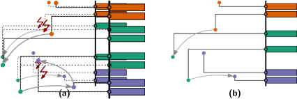
(b) An alternative set of ports to (10(a)) which allows for an admissible labeling.

Figure 10: An instance whose admissibility depends on the position of the ports.

By allowing the labels to slide along a sufficiently long vertical boundary line, we remove this limitation. To avoid the NP-hardness shown in Section 3.1 we require that all labels now have uniform height $h>0$.

In this section, we will first define for each site $s$ $\mathcal{O}(n)$ ports placed at multiples of $h$ away from $s$, building on an idea of Fink and Suri [14] that is visualized in Figure 11(a). After extending these ports by some small offset $\varepsilon>0$ we will prove in order: That if an instance has an admissible labeling, it also has an admissible (bend-minimal) labeling using these ports (Lemma 3.12), that if such an instance has an admissible labeling in which every leader has a minimum distance to every site, then there is a labeling with the same property using a slightly different set of ports, which also has equal or smaller total leader length (Lemma 3.14) and finally that these results in concert with Theorem 3.10 can be used to solve 1-CBL with uniform-height labels in polynomial time (Theorem 3.16).

Let $d$ be the smallest value one would need to add to a multiple of $h$ such that two sites are this far apart. Formally, this means $d\coloneqq\min_{s,s^{\prime}\in\mathcal{S}}\left(\left|y(s)-y(s^{\prime})\right|-qh\right)$, where $q=\left\lfloor\left|y(s)-y(s^{\prime})\right|/h\right\rfloor$. For the following arguments to work, we require $d>0$. However, this can easily be ensured by enforcing that the vertical distance $\left|y(s)-y(s^{\prime})\right|$ between any pair of sites $s$ and $s^{\prime}$ is not a multiple of $h$, which can be achieved by perturbating some sites slightly. As we then have $d>0$, we can select an $\varepsilon$ with $0<\varepsilon<d$. We now define a set of $\mathcal{O}(n^{2})$ ports s.t. there exists an admissible labeling on these (fixed) ports, if the instance with sliding ports possesses an admissible labeling. For each $s\in\mathcal{S}$, we define the following set.

$$\mathcal{P}(s)\coloneqq\{y(s)+ih,\ y(s)+ih\pm\varepsilon,\ y(s)-ih,\ y(s)-ih\pm\varepsilon\mid 0\leq i\leq n\}$$

Now, we define the set of canonical ports $\mathcal{P}(\mathcal{S})$ as $\mathcal{P}(\mathcal{S})\coloneqq\bigcup_{s\in\mathcal{S}}\mathcal{P}(s)$, some of which are visualized in Figure 11(b), and show the following.

(a) Ports induced by the sites as defined in [14].

(b) Ports from (11(a)) extended to the canonical ports.

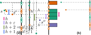
(c) The leader of $s$ crosses $s^{\prime}$ after moving all labels upwards. We only show the ports that arise from $s^{\prime}$.

Figure 11: The set of ports we construct in this section and (11(c)) their usage in the proofs.

Lemma 3.12.

Let $\mathcal{I}$ be an instance of 1-CBL with uniform-height labels, where the labels can slide along a vertical boundary line. If $\mathcal{I}$ possesses an admissible labeling, then there also exists one in which each port is from $\mathcal{P}(\mathcal{S})$.

Proof 3.13.

Our proof builds on arguments used by Fink and Suri for a similar result [14, Lemma 1] and we will call a maximal set of touching (but non-overlapping) labels a stack, following nomenclature used by Nöllenburg et al. [32].

Let $\mathcal{L}$ be an admissible labeling of $\mathcal{I}$ in which not all ports are from $\mathcal{P}(\mathcal{S})$. We will transform it into an admissible labeling $\mathcal{L}^{\prime}$ in which each port is from $\mathcal{P}(\mathcal{S})$. Throughout the proof, we will never change the order of the labels. Hence, if $\mathcal{L}$ respects the constraints, so does $\mathcal{L}^{\prime}$. Let $s_{t}$ and $s_{b}$ be the top-most and bottom-most sites in the instance, respectively. If there are labels that have their port strictly above $y(s_{t})$, we take them and arrange them as a single stack in the same order starting at the port $p$ with $y(p)=y(s_{t})+h$. These labels are all now placed at ports from $\mathcal{P}(\mathcal{S})$. A symmetric operation is performed with all labels that have their port strictly below $s_{b}$, which we place at the port $p$ with $y(p)=y(s_{b})-h$. Since these labels were initially placed above $s_{t}$ or below $s_{b}$, which is still the case afterwards, this cannot introduce any leader-site crossings. Furthermore, since we never move past sites or change the order of the labels, we cannot introduce leader-leader crossings.

Hence, the only labels that we have to deal with are those positioned between $s_{t}$ and $s_{b}$. For them, we proceed bottom-to-top as follows. We take the bottom-most not yet moved label $\ell$ and move it upwards until it either is positioned at a port from $\mathcal{P}(\mathcal{S})$ or hits another label $\ell^{\prime}$. In the former case, we stop. In the latter case, $\ell$ might not yet be at a port from $\mathcal{P}(\mathcal{S})$. To ensure that $\mathcal{L}^{\prime}$ is admissible, we “merge” these labels into a stack and move from now on this entire stack and thus all its labels simultaneously. We continue moving all the remaining not-yet-positioned labels in the same manner, until one of the above cases occurred for each of them. Observe that a label $\ell$ can never move past by a site since any site induces a port in $\mathcal{P}(\mathcal{S})$, i.e., in the worst case, we stop at a $p\in\mathcal{P}(\mathcal{S})$ with $y(p)=y(s)$ for some $s\in\mathcal{S}$. This may result in leaders crossing other sites if in $\mathcal{L}$ a leader $\lambda$ for a label $\ell$, originated at a site $s$, passes between a port of $\mathcal{P}(\mathcal{S})$ and a site $s^{\prime}\in\mathcal{S}$, $s\neq s^{\prime}$. If we then move $\ell$ upwards, the first port that we hit for $\ell$ might be the one directly induced by $s^{\prime}$, i.e., the port $p$, with $y(p)=y(s^{\prime})$. Depending on the position of $s^{\prime}$, i.e., if $x(s)<x(s^{\prime})$ holds, $\lambda$ now crosses $s^{\prime}$. To resolve this crossing, we take that label and the stack it belongs to, if there is one, and move it downwards until we hit a port from $\mathcal{P}(\mathcal{S})$. By our selection of $\varepsilon$, it is guaranteed that we will hit a port before we hit another site since there is at least one other port strictly between the end of the stack and any other site $s^{\prime\prime}$, as

$$0<\varepsilon<d\leq\left(\left|y(s^{\prime})-y(s^{\prime\prime})\right|-\left\lfloor\frac{\left|y(s^{\prime})-y(s^{\prime\prime})\right|}{h}\right\rfloor h\right)$$

holds, and we have ports at $y(s^{\prime})\pm\varepsilon$ and $y(s^{\prime\prime})\pm\varepsilon$. This is already indicated in Figure 11(b), but Figure 11(c) visualizes this in more detail with the orange ports. Note that $d\leq 1$ holds in Figure 11(c). Therefore, we have $\varepsilon<1$, and consequently $h+\varepsilon<h+d\leq h+2$, which is the (green) distance between the orange and the purple site. If we move all such (stacks of) labels simultaneously, we can never overlap with a placed label by moving downwards, but might merge with another stack already placed at ports from $\mathcal{P}(\mathcal{S})$. In the resulting labeling $\mathcal{L}^{\prime}$, each label is located at a port $p\in\mathcal{P}(\mathcal{S})$, and since we never changed the order of the labels when transforming $\mathcal{L}$ into $\mathcal{L}^{\prime}$, all constraints are still respected and $\mathcal{L}^{\prime}$ is admissible.

Observe that each site $s\in\mathcal{S}$ induces a port $p\in\mathcal{P}$ for which we have $y(s)=y(p)$. Hence, existence of a bend-minimal labeling on $\mathcal{P}(\mathcal{S})$ follows immediately. For length-minimal labelings, Figure 10 demonstrates that admissible instances without optimal labelings exist, as we can in Figure 10(b) always move the leader for the lower green site by a small $\varepsilon^{\prime}>0$ closer to the purple site, which reduces the length of the leaders, but guarantees that it remains admissible. To ensure the existence of length-minimal labelings, we enforce that the leaders maintain a minimum vertical distance of $0<d_{\min}$ to other sites. We define an alternative set of canonical ports $\mathcal{P}^{\prime}(\mathcal{S})$ that takes $d_{\min}$ into account.

$$\mathcal{P}^{\prime}(s) \coloneqq\{y(s)+qh,\ y(s)+qh\pm d_{\min},\ y(s)-qh,\ y(s)-qh\pm d_{\min}\mid 0\leq q\leq n\}$$

Equipped with $\mathcal{P}^{\prime}(\mathcal{S})\coloneqq\bigcup_{s\in\mathcal{S}}\mathcal{P}^{\prime}(s)$, we can show Lemma 3.14, which is a variant of Lemma 3.12.

Lemma 3.14.

Let $\mathcal{I}$ be an instance of 1-CBL with uniform labels, where the labels can slide along a vertical boundary line. If $\mathcal{I}$ possesses an admissible labeling $\mathcal{L}$ in which each leader maintains a minimum vertical distance $d_{\min}$ to other sites, then there also exists one in which each port is from $\mathcal{P}^{\prime}(\mathcal{S})$ and each leader still maintains the minimum vertical distance $d_{\min}$ to other sites. Furthermore, the leader length of $\mathcal{L}^{\prime}$ is not larger than that of $\mathcal{L}$.

Proof 3.15.

The crux of the proof is similar to the one for Lemma 3.12. However, we make two observations. Firstly, moving all labels that have their ports strictly above $y(s_{t})$ down can never increase the length of their leaders as they have their sites below their ports. A symmetric argument can be given for the labels that have their port below $y(s_{b})$. Secondly, in the initial labeling $\mathcal{L}$, all leaders maintain a vertical distance of at least $d_{\min}$ to other sites. Since we place a port this far away from each site $s$, we can never hit a site with our leaders while moving (stacks of) labels, i.e., we can never introduce a leader-site crossing.

The remainder of the proof is identical to the one for Lemma 3.12, except that we move (stacks of) labels always in a non-increasing direction with respect to the lengths of the involved leaders. This means that if in a stack more labels have their site above the respective ports, we move the stack upwards, and vice versa. We break ties arbitrarily. If this leads to two stacks touching before they reach ports from $\mathcal{P}^{\prime}(\mathcal{S})$, we merge them and move the single resulting stack in the same manner. As already observed by Fink and Suri [14], we never increase the overall leader length and this operations must eventually stop. Thus, for the labeling $\mathcal{L}^{\prime}$ that we eventually obtain, we know that the sum of the leader lengths can be at most as large as the one in the initial labeling $\mathcal{L}$.

Note that $\mathcal{P}^{\prime}(\mathcal{S})$ can contain ports for which leaders would not satisfy our requirement on a vertical distance of at least $d_{\min}$ to other sites. However, observe that we never move past a port while sliding labels. Since we started with an admissible labeling where the leaders maintain the distance $d_{\min}$ to other sites, and created ports that are that far away from the sites, this cannot result in a labeling violating our requirement of the leaders having a minimum vertical distance of $d_{\text{min}}$ to other sites. This criterion can also be patched into the admissibility-checks without affecting the running time. Finally, having this additional requirement is not a limitation, as this is already often required in real-world labelings [31].

Theorem 3.16.

1-CBL, with uniform-height labels, can be solved in $\mathcal{O}(n^{11}\log n+k+\sum_{\mathcal{G}\in\mathscr{G}}\left|\mathcal{G}\right|)$ time and $\mathcal{O}(n^{6})$ space.

Proof 3.17.

First, note that for our sets of canonical ports we have $\mathcal{O}(\left|\mathcal{P}(\mathcal{S})\right|)=\mathcal{O}(\left|\mathcal{P}^{\prime}(\mathcal{S})\right|)=\mathcal{O}(n^{2})$. Furthermore, we have shown in Lemmas 3.12 and 3.14 that these ports are sufficient for obtaining an admissible, bend-, and length-minimal labeling, if there exists one at all. Therefore, we have reduced the 1-CBL problem with uniform-height labels to the 1-CBL problem with fixed ports (and uniform height labels). Thus, we can use our DP-Algorithm from Section 3.2 and obtain Theorem 3.16 by plugging in $m=\mathcal{O}(n^{2})$ in Theorem 3.10.

4 Experimental Evaluation of the DP-Algorithm for Fixed Ports

From a theoretical point of view, Theorem 3.10 shows that 1-CBL can for fixed ports be solved in polynomial time. However, the large (asymptotic) running time of the algorithm leads one to assume that it has little practical relevance. Given that the problem is motivated from real-world applications, we now seek to experimentally evaluate the approach on synthetic and real-world instances. In contrast to our description from Section 3.2, which allows for non-uniform height labels and more general optimization functions, we will in the following stick to uniform-height labels and minimize the length of the leaders. We will give an overview of the experiments and its results, but refer to Depian’s Master’s thesis [12] for full details.

Implementation Details.

We implemented our DP in C++17 to find a leader-length minimal labeling for uniform-height ($20$ pixels) labels on fixed ports.

For the PQ-A-Graphs, we used a PC-Tree implementation by Fink et al. [15] that outperforms existing PQ-Tree implementations as starting point. We make also use of a range tree implementation by Weihs [39] that was already used in the literature [38]. Furthermore, we implement two ideas to speed up the running time of our algorithm for many real-world instances. Note that each of them does not decrease the asymptotic time complexity of the algorithm and has no influence on its correctness.

Our first idea concerns the computation of the least common ancestor of two leaves. As this information is accessed several times in the algorithm, we noticed that pre-computing this information for all pairs of leaves had a positive effect on the measured running time.

Our second idea aims at avoiding checking whether the leader $\lambda_{L}=(s_{L},p_{L})$ would respect the constraints, if we can already infer this information from previously performed checks. Note that this circumvents (re-) running the time-expensive procedure ${\textsc{RespectsConstraints}}(I,\mathcal{T},\lambda_{L})$. More concretely, assume that the bounding box of the sites in a sub-instance $I=(s_{1},p_{1},s_{2},p_{2})$ is identical to the one in a sub-instance $I^{\prime}=(s_{1},p_{1}^{\prime},s_{2},p_{2}^{\prime})$. As this bounding box comprises the same sites and both sub-instances are described by $s_{1}$ and $s_{2}$, everything that affects the outcome of ${\textsc{RespectsConstraints}}(I,\mathcal{T},\lambda_{L})$ for $\lambda_{L}=(s_{L},p_{L})$ is identical, given that $s_{L}$ is the leftmost site (in both sub-instances) and we have $p_{L}\in{\mathcal{P}}(I)\cap{\mathcal{P}}(I^{\prime})$. As a consequence, we can use memoization and just (re-) use the result from, for example, ${\textsc{RespectsConstraints}}(I^{\prime},\mathcal{T},\lambda_{L})$. We visualize this idea in Figure 12 and want to mention that it is inspired by the practical considerations made by Niedermann et al. [31] to speed up their contour labeling algorithm.

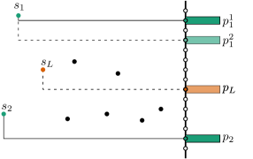
Figure 12: No matter if we have the sub-instance $I=(s_{1},p_{1}^{1},s_{2},p_{2})$ or $I^{\prime}=(s_{1},p_{1}^{2},s_{2},p_{2})$, if we label $s_{L}$ at $p_{L}$ the leader $\lambda_{L}=(s_{L},p_{L})$ will in both sub-instances either respect the constraints or do not respect them.

Furthermore, we implemented the ILP-formulation from the user study by Barth et al. [1], which we call in the following Naïve-ILP, and use it as a reference for the running time of our DP-algorithm. Note that this should only simulate a “textbook” implementation of a labeling algorithm and does not claim to be the most efficient way to obtain a leader-length minimal labeling on fixed ports. Furthermore, the ILP is unaware of our constraints.

Datasets.

We used four datasets, where three of them are based on the following real-world data. The cities dataset contains instances with the $n\in\{10,15,20,25,30,35,40,45\}$ largest cities from Austria, Germany, and Italy, respectively, obtained from simplemaps.com [34]. For each combination of country and $n$, we create one instance without constraints, which we use for the ILP, and group the cities in the other instances according to the administrative regions of the respective country. In addition, in one of the instances with the groups, we order the cities in each group according to their administrative status (create so-called intra-group constraints). A fourth instance is created where we order the groups according to their population computed from the cities in the instance (create so-called inter-group constraints). To do the latter, we select a representative site from each group and insert the corresponding ordering constraints. We create multiple variants of this dataset, each with a different number of ports. In cities-2x, each instance has $m=2n$ many ports, and cities-90 defines 90 ports per instance. For these two datasets, we maintain a distance of at least twenty pixels, the label height, between two ports. For cities-10px, we perform differently. We take the initial height of the boundary and place a port every ten pixels. If this leads to too few ports, we add more ports accordingly, thus increasing the height of the boundary. This approach led to 71 ports for the Austrian cities and 128 and 130 for the German and Italian cities, respectively, independent of the number of cities in the instance.

The ports dataset is a variation of the cities dataset(s), where we consider the $n=25$ largest cities from the countries. For each combination of country and constraints, we create different instances where we vary the number of ports $m$. We use $m\in\{\lceil xn\rceil\mid x\in\{1.0,1.1,\dots,2.9,3.0\}\}$ and enforce a distance of at least ten pixels between two ports.

Finally, the last real-world dataset contains five instances obtained from the Sobotta atlas of human anatomy [37] that Niedermann et al. used to evaluate the performance of their contour labeling algorithm [31]. These instances are enriched with grouping and ordering constraints as described in Table 1. Note that the book uses contour labeling for their illustrations. Therefore, we selected the instances such that we maintain feasibility also under the boundary labeling model. Similar to Niedermann et al., we place a port every ten pixels.

Table 1: Size of the instances based on illustrations from the Sobotta atlas of human anatomy [37].

Figure	$n$	$m$	$k$	$r$	Definition of Constraints
Fig. 8.30	11	44	3	0	Groups based on colored regions or curly brackets enclosing labels.
Fig. 8.81	9	60	0	7	A nerve branching off another nerve should be labeled below its “parent”.
Fig. 9.23	11	53	3	0	Overlapping groups based on explicit curly brackets or colored regions.
Fig. 12.33	9	38	3	0	Grouping based on colored regions. Sites on the boundary of two regions are in both regions, i.e., groups overlap.
Fig. 12.59	19*	62	3	6	Grouping based on curly brackets, ordering based on Roman letters next to some labels.

• The original figure contains 31 sites labeled on the left and right sides of the illustration. However, we took only the sites labeled on the left side.

We furthermore used a synthetic dataset containing random instances. However, the datasets based on real-world data gave us the most insight and we thus discuss in this paper only the results for them. A description of and the results for the fourth dataset can be found in Depian’s Master’s thesis [12]. All datasets together contain 750 instances.

Experimental Setup.

Most instances were solved on a compute cluster with Intel Xeon E5-2640 v4 10-core processors at 2.40GHz that have access to 160 GB of RAM. We set a hard time limit of twenty hours per instance and a hard memory limit of 96 GB. Neither of the limits was exceeded. To simulate a real-world setting, we computed the instances from the book on an off-the shelf laptop with an Intel Core i5-8265U 4-core processor at 1.60GHz. There, we had, inside a WSL2 environment, access to 7.8 GB of RAM.

Results.

A detailed discussion of the results can be found in the Master’s thesis [12], but at a glance the experiments revealed that, apart from the dataset based on the book, each dataset contains, on average, only thirty percent feasible instances. In particular, those instances that contained grouping and ordering constraints were often infeasible. Comparing the feasible instances with both types of constraints to their counterpart without ordering constraints revealed that the former only have a negligible higher leader length. This gives the impression that ordering constraints are well suited for enforcing locally limited orders but should not be used to put labels for sites far away into relation. As the instances based on the book were feasible, but not all real-world instances, we conclude that we should not only consider the semantics of sites but also their (geometric) position when defining constraints.

We present in Figures 13, 14 and 2 the running times and running time plots for our implementation. For the cities dataset(s), we report in Figure 13 the running time plots. Figure 13(a) shows the running times for the instances that contain only grouping constraints. Furthermore, we plot the average running time of the ILP together with the range of measured running times as reference.

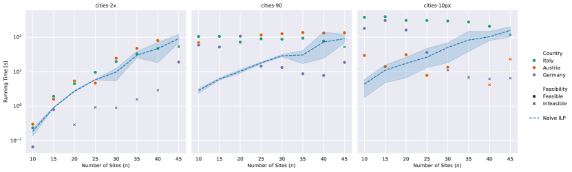
(a) Running time for instances that only contain grouping constraints.

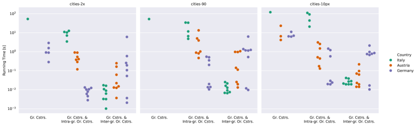
(b) Time required to detect infeasible instances.

Figure 13: Running time on the cities datasets ($\log$-plots). Gr. stands for grouping and Or. for ordering constraints (abbreviated as Cstrs.)

As many of the instances with grouping and ordering constraints were infeasible, we refrain from plotting their running times in detail. However, they are included in Figure 13(b), where we plot the running times of all infeasible instances. For the ports dataset, we plot in Figure 14 the running times. Figure 14(a) shows the running times of the instances with only grouping constraints and contains, as for the cities datasets, the running time of the ILP as a reference. We plot the running times of all infeasible instances in Figure 14(b).

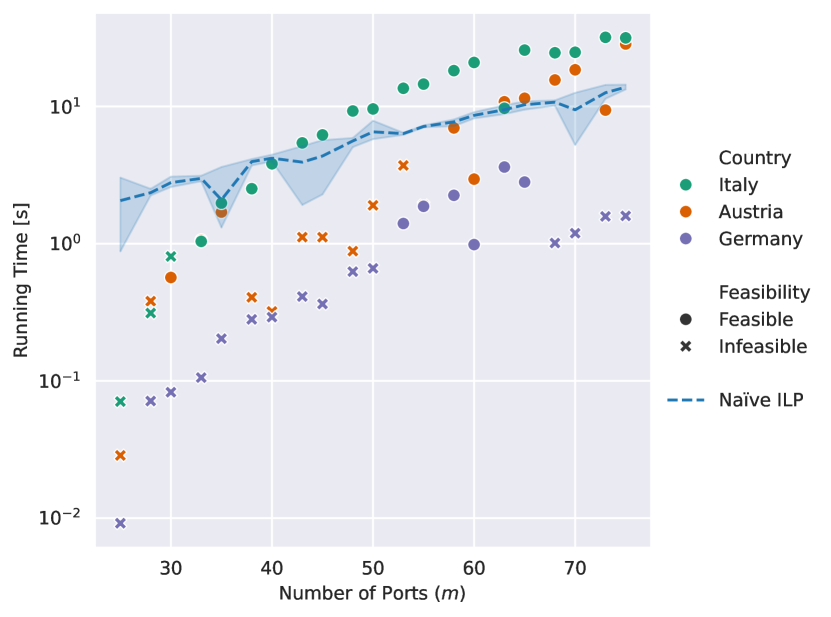
(a) Running time for instances that only contain grouping constraints.

(b) Time required to detect infeasible instances.

Figure 14: Running time on the ports dataset ($\log$-plots). Gr. stands for grouping and Or. for ordering constraints (abbreviated as Cstrs.).

Table 2 contains the running times for our solver and the ILP on the instances from the Sobotta atlas of human anatomy.

Table 2: Running time (in seconds) of our algorithms on the instances from the Sobotta atlas of human anatomy.

		Our DP-Algorithm
Instance	Naïve ILP	Total	Of Which Bookkeeping*
Fig. 8.30	0.7922	0.6084	0.0003
Fig. 8.81	0.4295	0.3700	0.0003
Fig. 9.23	0.5023	0.3658	0.0004
Fig. 12.33	0.2519	0.0418	0.0003
Fig. 12.59	2.4632	3.6388	0.0006

• This includes everything but filling the DP-Table $D$.

From the plots and measurements, we can observe that our algorithm is for small to medium-sized instances fast enough to compute a labeling in a few seconds or classify them as infeasible, even on an off-the-shelf laptop (Table 2). On the other hand, if the instance is large, the running time can be seen as a limitation of our approach. In particular, we could measure a running time of up to seven minutes for the largest instances (Figure 13(a)). On a positive note, infeasibility was for most instances detected within ten seconds (Figures 13(b) and 14(b)). Furthermore, we observed that the running time seems to be more dependent on the number of ports than on the number of sites.

Finally, the ports had not only an influence on the running time. We could in addition observe that the quality and feasibility of the labeling strongly depend on them, which justifies our considerations in Section 3.3 for a setting without a pre-determined set of ports.

5 Conclusion

We analyzed the support of grouping and ordering constraints in boundary labeling. While finding an admissible labeling is (weakly) NP-hard, efficient algorithms for 1-sided instances with fixed ports or uniform-height labels exist. Natural next steps would be to consider the inclusion of soft constraints, i.e., a setting where even if not all constraints can be adhered to, we aim to maximize the number of satisfied constraints. Since often features other than points are labeled, it is also worth studying a variant of this problem with uncertain or variable site locations. Similarly, the support of other leader styles, which have been established for boundary labeling, or entire other labeling styles, should be investigated. Finally, the visual quality of the produced labeling should be experimentally evaluated.

References

- [1] Lukas Barth, Andreas Gemsa, Benjamin Niedermann, and Martin Nöllenburg. On the readability of leaders in boundary labeling. Information Visualization, 18(1):110–132, 2019. doi:10.1177/1473871618799500.
- [2] Michael A. Bekos, Sabine Cornelsen, Martin Fink, Seok-Hee Hong, Michael Kaufmann, Martin Nöllenburg, Ignaz Rutter, and Antonios Symvonis. Many-to-One Boundary Labeling with Backbones. Journal of Graph Algorithms and Applications (JGAA), 19(3):779–816, 2015. doi:10.7155/jgaa.00379.
- [3] Michael A. Bekos, Michael Kaufmann, Martin Nöllenburg, and Antonios Symvonis. Boundary Labeling with Octilinear Leaders. Algorithmica, 57(3):436–461, 2010. doi:10.1007/s00453-009-9283-6.
- [4] Michael A. Bekos, Michael Kaufmann, Antonios Symvonis, and Alexander Wolff. Boundary labeling: Models and efficient algorithms for rectangular maps. Computational Geometry, 36(3):215–236, 2007. doi:10.1016/j.comgeo.2006.05.003.
- [5] Michael A. Bekos, Benjamin Niedermann, and Martin Nöllenburg. External Labeling: Fundamental Concepts and Algorithmic Techniques. Synthesis Lectures on Visualization. Springer, 2021. doi:10.1007/978-3-031-02609-6.
- [6] Michael A. Bender and Martin Farach-Colton. The LCA Problem Revisited. In Proc. 4th Latin American Symposium on Theoretical Informatics (LATIN), volume 1776 of Lecture Notes in Computer Science (LNCS), pages 88–94. Springer, 2000. doi:10.1007/10719839_9.
- [7] Marc Benkert, Herman J. Haverkort, Moritz Kroll, and Martin Nöllenburg. Algorithms for Multi-Criteria Boundary Labeling. Journal of Graph Algorithms and Applications (JGAA), 13(3):289–317, 2009. doi:10.7155/jgaa.00189.
- [8] Satyam Bhuyan and Santanu Mukherjee (sciencefacts.net). Layers of the Sun, 2023. Accessed on 2023-09-07. URL: https://www.sciencefacts.net/layers-of-the-sun.html.
- [9] Kellogg S. Booth and George S. Lueker. Testing for the Consecutive Ones Property, Interval Graphs, and Graph Planarity Using PQ-Tree Algorithms. Journal of Computer and System Sciences (JCSS), 13(3):335–379, 1976. doi:10.1016/S0022-0000(76)80045-1.
- [10] Mary Helen Briscoe. A Researcher’s Guide to Scientific and Medical Illustrations. Springer Science & Business Media, 1990. doi:10.1007/978-1-4684-0355-8.
- [11] Mark de Berg, Otfried Cheong, Marc J. van Kreveld, and Mark H. Overmars. Computational Geometry: Algorithms and Applications, 3rd Edition. Springer, 2008.
- [12] Thomas Depian. Grouping and Ordering Constraints in Boundary Labeling. Master’s thesis, TU Wien, 2023. doi:10.34726/HSS.2023.113812.
- [13] Martin Fink, Jan-Henrik Haunert, André Schulz, Joachim Spoerhase, and Alexander Wolff. Algorithms for Labeling Focus Regions. IEEE Transactions on Visualization and Computer Graphics, 18(12):2583–2592, 2012. doi:10.1109/TVCG.2012.193.
- [14] Martin Fink and Subhash Suri. Boundary Labeling with Obstacles. In Proc. 28th Canadian Conference on Computational Geometry (CCCG), pages 86–92. Simon Fraser University, 2016.
- [15] Simon D. Fink, Matthias Pfretzschner, and Ignaz Rutter. Experimental Comparison of PC-Trees and PQ-Trees. In Proc. 29th European Symposium on Algorithms (ESA), volume 204 of Leibniz International Proceedings in Informatics (LIPIcs), pages 43:1–43:13. Schloss Dagstuhl - Leibniz-Zentrum für Informatik, 2021. doi:10.4230/LIPIcs.ESA.2021.43.
- [16] Delbert Fulkerson and Oliver Gross. Incidence matrices and interval graphs. Pacific Journal of Mathematics, 15(3):835–855, 1965.
- [17] Michael R. Garey and David S. Johnson. Computers and Intractability: A Guide to the Theory of NP-Completeness. W. H. Freeman, 1979.
- [18] Sven Gedicke, Lukas Arzoumanidis, and Jan-Henrik Haunert. Automating the external placement of symbols for point features in situation maps for emergency response. Cartography and Geographic Information Science (CaGIS), 50(4):385–402, 2023. doi:10.1080/15230406.2023.2213446.
- [19] Sven Gedicke, Annika Bonerath, Benjamin Niedermann, and Jan-Henrik Haunert. Zoomless Maps: External Labeling Methods for the Interactive Exploration of Dense Point Sets at a Fixed Map Scale. IEEE Transactions on Visualization and Computer Graphics, 27(2):1247–1256, 2021. doi:10.1109/TVCG.2020.3030399.
- [20] Andreas Gemsa, Jan-Henrik Haunert, and Martin Nöllenburg. Multirow Boundary-Labeling Algorithms for Panorama Images. ACM Transactions on Spatial Algorithms and Systems (TSAS), 1(1):1:1–1:30, 2015. doi:10.1145/2794299.
- [21] Timo Götzelmann, Knut Hartmann, and Thomas Strothotte. Agent-Based Annotation of Interactive 3D Visualizations. In Proc. 6th International Symposium on Smart Graphics (SG), volume 4073 of Lecture Notes in Computer Science (LNCS), pages 24–35. Springer, 2006. doi:10.1007/11795018_3.
- [22] Timo Götzelmann, Knut Hartmann, and Thomas Strothotte. Contextual Grouping of Labels. In Proc. 17th Simulation und Visualisierung (SimVis), pages 245–258. SCS Publishing House e.V., 2006.
- [23] Bernhard Haeupler and Robert Endre Tarjan. Planarity algorithms via pq-trees (extended abstract). Electronic Notes in Discrete Mathematics, 31:143–149, 2008. doi:10.1016/J.ENDM.2008.06.029.
- [24] Wen-Lian Hsu and Ross M. McConnell. PC trees and circular-ones arrangements. Theoretical Computer Science, 296(1):99–116, 2003. doi:10.1016/S0304-3975(02)00435-8.
- [25] Haitao Jiang, Hong Liu, Cédric Chauve, and Binhai Zhu. Breakpoint distance and PQ-trees. Information and Computation, 275:104584, 2020. doi:10.1016/j.ic.2020.104584.
- [26] Philipp Kindermann, Benjamin Niedermann, Ignaz Rutter, Marcus Schaefer, André Schulz, and Alexander Wolff. Multi-sided Boundary Labeling. Algorithmica, 76(1):225–258, 2016. doi:10.1007/s00453-015-0028-4.
- [27] Pavel Klavík, Jan Kratochvíl, Yota Otachi, Toshiki Saitoh, and Tomás Vyskocil. Extending Partial Representations of Interval Graphs. Algorithmica, 78(3):945–967, 2017. doi:10.1007/s00453-016-0186-z.
- [28] Jonathan Klawitter, Felix Klesen, Joris Y. Scholl, Thomas C. van Dijk, and Alexander Zaft. Visualizing Geophylogenies - Internal and External Labeling with Phylogenetic Tree Constraints. In Proc. 12th International Conference Geographic Information Science (GIScience), volume 277 of Leibniz International Proceedings in Informatics (LIPIcs), pages 5:1–5:16. Schloss Dagstuhl - Leibniz-Zentrum für Informatik, 2023. doi:10.4230/LIPIcs.GIScience.2023.5.
- [29] Konrad Mühler and Bernhard Preim. Automatic Textual Annotation for Surgical Planning. In Proc. 14th International Symposium on Vision, Modeling, and Visualization (VMV), pages 277–284. DNB, 2009.
- [30] Benjamin Niedermann and Jan-Henrik Haunert. Focus+context map labeling with optimized clutter reduction. International Journal of Cartography, 5(2–3):158–177, 2019. doi:10.1080/23729333.2019.1613072.
- [31] Benjamin Niedermann, Martin Nöllenburg, and Ignaz Rutter. Radial Contour Labeling with Straight Leaders. In Proc. 10th IEEE Pacific Visualization Symposium (PacificVis), Lecture Notes in Computer Science (LNCS), pages 295–304. IEEE Computer Society, 2017. doi:10.1109/PACIFICVIS.2017.8031608.
- [32] Martin Nöllenburg, Valentin Polishchuk, and Mikko Sysikaski. Dynamic one-sided boundary labeling. In Proc. 18th ACM SIGSPATIAL International Conference on Advances in Geographic Information Systems (GIS), pages 310–319. Association for Computing Machinery (ACM), 2010. doi:10.1145/1869790.1869834.
- [33] Thomas J. Schaefer. The Complexity of Satisfiability Problems. In Proc. 10th Symposium on the Theory of Computing (STOC), pages 216–226. Association for Computing Machinery (ACM), 1978. doi:10.1145/800133.804350.
- [34] SimpleMaps.com. simplemaps: Interactive Maps & Data, 2023. Accessed on 2023-10-13. URL: https://simplemaps.com/.
- [35] Markus Tatzgern, Denis Kalkofen, and Dieter Schmalstieg. Dynamic Compact Visualizations for Augmented Reality. In Proc. 20th IEEE Conference on Virtual Reality and 3D User Interfaces (VR), pages 3–6. IEEE Computer Society, 2013. doi:10.1109/VR.2013.6549347.
- [36] Ian Vollick, Daniel Vogel, Maneesh Agrawala, and Aaron Hertzmann. Specifying label layout style by example. In Proc. 20th ACM Symposium on User Interface Software and Technology (UIST), pages 221–230. Association for Computing Machinery (ACM), 2007. doi:10.1145/1294211.1294252.
- [37] Jens Waschke and Friedrich Paulsen. Sobotta Atlas of Human Anatomy: Head, Neck and Neuroanatomy, volume 3. Elsevier, 15th edition edition, 2013.
- [38] Luca Weihs, Mathias Drton, and Nicolai Meinshausen. Symmetric rank covariances: a generalized framework for nonparametric measures of dependence. Biometrika, 105(3):547–562, 2018. doi:10.1093/biomet/asy021.
- [39] Luca (Lucaweihs) Weihs. GitHub: C++ Range Tree Data Structure, 2020. Accessed on 2023-10-29. URL: https://github.com/Lucaweihs/range-tree.