Concentration Inequalities, Dynamical Activity, and Trade-off Relations

Abstract

We present a concentration inequality in stochastic thermodynamics that provides a lower bound for the probability distribution of observables in Markov processes, where the lower bound includes the dynamical activity, a central thermodynamic quantity in trade-off relations. The derived inequality is called the thermodynamic concentration inequality. As a first corollary of the thermodynamic concentration inequality, by combining it with the Markov inequality, we derive an upper bound on the expectation of an observable given its maximum. Furthermore, as a second corollary, we obtain a generalization of the thermodynamic uncertainty relation, where the first and second moments of the original relation are replaced by the $p$-norm. These corollaries are valid for an arbitrary Markov process with time-dependent transition rates and for an arbitrary initial probability distribution. The thermodynamic concentration inequality provides the foundation for discovering trade-off relations.

Introduction.—In recent years, the concept of trade-off relations is gaining considerable interest in thermodynamics and quantum mechanics. The thermodynamic uncertainty relation (TUR) [1, 2, 3, 4, 5, 6, 7, 8, 9, 10, 11, 12, 13, 14, 15, 16, 17, 18, 19, 20, 21] (see [22] for a review) and the speed limit [23, 24, 25, 26, 27, 28, 29, 30, 31, 32, 33, 34] (see [35] for a review) are essential components of the trade-off relations. The TUR implies that a thermodynamic machine needs a larger thermodynamic input to achieve a higher level of precision. The speed limit suggests that making more significant or faster changes to the state requires more thermodynamic or quantum resources. Essentially, these relations illustrate the principle that there are no effortless gains in the physical world.

Concentration inequalities estimate the degree to which a random variable deviates from a certain value [36]. They are indispensable tools in the field of probability theory and are widely used in numerous areas, including machine learning, statistics, and optimization. The major advantage of concentration inequalities lies in their generality. Many concentration inequalities hold universally because they make very few assumptions about random variables. In this Letter, we derive a concentration inequality in stochastic thermodynamics that provides a lower bound for the probability distribution of general observables in Markov processes. We refer to the obtained relation as the thermodynamic concentration inequality (Theorem 1). The lower bound of this inequality comprises dynamical activity, which is a central quantity in the thermodynamic uncertainty relations [3, 5] and the classical speed limits [31].

As corollaries of the thermodynamic concentration inequality, we derive several trade-off relations by combining it with other concentration inequalities. We first employ the Markov inequality, which provides an upper bound for the probability that a non-negative random variable is equal to or exceeds a certain positive constant, to obtain the first corollary. The first corollary (Corollary 1) bounds the expected value of a general observable, given that the observable is bounded from above by a constant. Moreover, as a second corollary (Corollary 2), we obtain a trade-off relation for the norm of the observable by using the Petrov inequality [37], which is a generalization of the Paley-Zygmund inequality [38]. The Paley-Zygmund inequality establishes a lower bound for the probability that a nonnegative random variable surpasses a specific value based on the first two moments of the variable. The obtained relation is reminiscent of a TUR recently derived in Ref. [39]. Although the TURs reported so far concern the first and second moments, the derived bound considers the $p$-norm. We show that the result shown in the second corollary is more general and stronger than the previously shown TUR [39]. Due to the generality of the concentration inequalities, the relations shown in these corollaries exhibit a very high level of generality. In addition, we perform computer simulations to validate the theorem and corollaries. Information inequalities, such as the Cramér-Rao inequality, have been widely used in TURs and speed limits. Here, our derivation of the thermodynamic concentration inequality opens the way to discovering new trade-off relations through the integration of the derived inequality with other concentration inequalities.

Methods.—We consider a classical Markov process comprising $M$ states, denoted as a set $\mathfrak{B}=\{B_{1},B_{2},\cdots,B_{M}\}$. Let $P(\nu;t)$ be the probability that the state equals $B_{\nu}$ at time $t$ and let $W_{\nu\mu}$ be the transition rate from state $B_{\mu}$ to state $B_{\nu}$. The time evolution of $\mathbf{P}(t)=[P(1;t),\ldots,P(M;t)]^{\top}$ is subject to the following master equation:

$$\frac{d\mathbf{P}(t)}{dt}=\mathbf{W}\mathbf{P}(t),$$ (1)

where $\mathbf{W}=[W_{\nu\mu}]$ and the diagonal entries of $\mathbf{W}$ are defined by $W_{\nu\nu}\equiv-\sum_{\mu(\neq\nu)}W_{\mu\nu}$. Along with the ensemble average description, in stochastic thermodynamics, we are often interested in the trajectory-level description. Let $\omega_{\tau}$ be a trajectory of the Markov process within the time interval $[0,\tau]$ ($\tau>0$). Suppose that a trajectory consists of $K$ jump events. Let us denote the timestamp of the $l$th jump as $t_{l}$, where $l\in\{0,1,\cdots,K\}$ (here $t_{0}=0$, $t_{K+1}=\tau$). Furthermore, we define $B_{\mu_{l}}$ as the state that follows immediately after the $l$th jump, where the trajectory begins with $B_{\mu_{0}}$. Then the probability of a trajectory $\omega_{\tau}$ is given by

$$\mathcal{P}(\omega_{\tau};\mathbf{W})=P(\mu_{0};0)\mathcal{P}(\omega_{\tau}|\mu_{0};\mathbf{W}),$$ (2)

where $\mathcal{P}(\omega_{\tau}|\mu_{0};\mathbf{W})$ is the conditional probability of $\omega_{\tau}$ given the initial state $B_{\mu_{0}}$. It is expressed as

$$\mathcal{P}(\omega_{\tau}|\mu_{0};\mathbf{W})=\prod_{l=1}^{K}W_{\mu_{l}\mu_{l-1}}e^{-\sum_{l=0}^{K}\left(t_{l+1}-t_{l}\right)R\left(\mu_{l}\right)},$$ (3)

where $R(\mu)\equiv\sum_{\nu(\neq\mu)}W_{\nu\mu}$. In Eq. (2), we explicitly represent the dependence of the trajectory probability on the transition rate matrix $\mathbf{W}$ for later use.

Let $N(\omega_{\tau})$ be an observable of the trajectory $\omega_{\tau}$, which is the key quantity in this Letter. The observable $N(\omega_{\tau})$ can be arbitrary as long as the following condition is satisfied:

$$N(\omega_{\varnothing})=0,$$ (4)

where $\omega_{\varnothing}$ is a trajectory with no jump. Equation (4) simply states that the observable should vanish when there is no jump. This condition is a generalization of the counting observable, which counts the number of jump events (see Eq. (5)), and was used in Refs. [18, 40, 39]. Hereafter, we will simplify the notation $N(\omega_{\tau})$ to $N(\tau)$. A typical example of $N(\tau)$ that satisfies the condition of Eq. (4) is the counting observable:

$$N(\tau)=\sum_{\mu,\nu,\mu\neq\nu}C_{\nu\mu}N_{\nu\mu}(\tau),$$ (5)

where $\mathbf{C}=[C_{\nu\mu}]$ is the real weight matrix and $N_{\nu\mu}(\tau)$ is the number of jump events from $B_{\mu}$ to $B_{\nu}$ within time interval $[0,\tau]$. For instance, the TUR of Ref. [3] concerns the counting observable of Eq. (5). Furthermore, when condition $C_{\nu\mu}=-C_{\mu\nu}$ is satisfied, Eq. (5) can represent the thermodynamic current, which is a key quantity in the original TUR [1, 2]. Given that $\omega_{\tau}$ is a random variable, $N(\tau)$ is also a random variable. Therefore, we can think of its probability distribution $P(N(\tau))$.

Next, we define the dynamical activity which is a thermodynamic quantity often considered in the TURs [3, 5] and the classical speed limits [31, 41]. The time-integrated dynamical activity within $[0,\tau]$ is defined by

$$\mathcal{A}(\tau)\equiv\int_{0}^{\tau}\sum_{\nu,\mu\,(\nu\neq\mu)}P_{\mu}(t)W_{\nu\mu}(t)dt.$$ (6)

Here, $\mathcal{A}(\tau)$ represents the average frequency of jump events occurring during the time interval $[0,\tau]$. Therefore, $\mathcal{A}(\tau)$ quantifies the activity of the Markov process. Here, we claim that the dynamical activity $\mathcal{A}(\tau)$ and probability $P(N(\tau)=0)$ are related via the inequality, which is stated as follows.

Theorem 1.

For $0\leq(1/2)\int_{0}^{\tau}\sqrt{\mathcal{A}(t)}/t\,dt\leq\pi/2$, the thermodynamic concentration inequality holds:

$$\cos\left[\frac{1}{2}\int_{0}^{\tau}\frac{\sqrt{\mathcal{A}(t)}}{t}dt\right]^{2}\leq P(N(\tau)=0).$$ (7)

A proof of Theorem 1 is shown in the Appendix. For $\tau$ outside the condition $0\leq(1/2)\int_{0}^{\tau}\sqrt{\mathcal{A}(t)}/t\,dt\leq\pi/2$, the trivial inequality $0\leq P(N(\tau)=0)$ holds. Theorem 1 is the main result of this Letter because it serves as the key ingredient to obtain trade-off relations through other concentration inequalities. Equation (7) can be equivalently expressed by $\sin\left[(1/2)\int_{0}^{\tau}\sqrt{\mathcal{A}(t)}/t\,dt\right]^{2}\geq P(|N(\tau)|>0)$, which estimates the deviation of the probability that $|N(\tau)|$ exceeds $0$. When the dynamical activity $\mathcal{A}(\tau)$ is higher, it is naturally expected that the probability $P(N(\tau)=0)$ becomes lower because there are more jumps. Theorem 1 demonstrates this notion quantitatively.

We perform numerical simulations to validate Theorem 1. We prepare random Markov processes and calculate $P(N(\tau)=0)$ as a function of $\cos\left[(1/2)\int_{0}^{\tau}\sqrt{\mathcal{A}(t)}/t\,dt\right]^{2}$ for the random realizations. Here, we use the counting observable [Eq. (5)] with $C_{\nu\mu}=1$ for all $\mu$ and $\nu$, which simply counts the number of jump events within $[0,\tau]$. The random realizations are plotted by circles in Fig. 1(a). In Fig. 1(a), the dashed line denotes the equality case in Eq. (7). We see that all circles appear to be above the dashed line, thus numerically validating Theorem 1. From the simulation, Eq. (7) is tighter for a larger value of $P(N(\tau)=0)$, which implies that Eq. (7) provides a more precise estimate for $P(N(\tau)=0)$ for shorter $\tau$.

Next, we obtain the corollaries of Theorem 1 by combining it with other concentration inequalities. The most common concentration inequality is the Markov inequality. Let $X$ be a random variable and let $\mathbb{E}[X]$ be the expectation of $X$. For a positive constant $a$, the Markov inequality states

$$P(|X|\geq a)\leq\frac{\mathbb{E}\left[|X|\right]}{a}.$$ (8)

The Markov inequality is a fundamental relation in probability theory and statistics. It provides an upper bound on the probability that a nonnegative function of a random variable is equal to or greater than a specific positive constant. This theorem serves as a fundamental tool because of its simplicity and generality; it does not require knowledge of the probability distribution, just its mean. Using the Markov inequality, we can derive an upper bound for $\mathbb{E}[|N(\tau)|]$ as follows.

Corollary 1.

Let $N_{\mathrm{max}}$ be the maximum of $|N(\tau)|$. Then, for $0\leq(1/2)\int_{0}^{\tau}\sqrt{\mathcal{A}(t)}/t\,dt\leq\pi/2$, the following relation holds:

$$\mathbb{E}[|N(\tau)|]\leq N_{\max}\sin\left[\frac{1}{2}\int_{0}^{\tau}\frac{\sqrt{\mathcal{A}(t)}}{t}dt\right]^{2}.$$ (9)

A proof of Corollary 1 is based on application of Theorem 1 to the Markov inequality, which is shown in the Appendix. Corollary 1 holds for any Markov processes with time-dependent transition rates and general observables that satisfy Eq. (4). Equation (9) is similar to the bound derived in Ref. [42]. While the bound in Ref. [42] provides an upper bound for $|\mathbb{E}[N(\tau)]-\mathbb{E}[N(0)]|$, Eq. (9) does so for $\mathbb{E}[|N(\tau)|]$. Furthermore, Eq. (9) is stronger than the bound presented in Ref. [42].

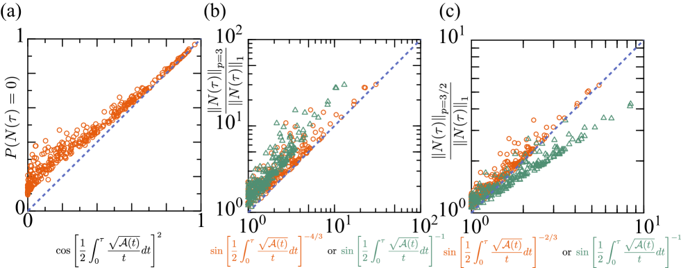
Figure 1: (a) Random simulation of Theorem 1. $P(N(\tau)=0)$ is plotted as a function of $\cos\left[(1/2)\int_{0}^{\tau}\sqrt{\mathcal{A}(t)}/t\,dt\right]^{2}$. Here, we exclude points with vanishing $\cos\left[(1/2)\int_{0}^{\tau}\sqrt{\mathcal{A}(t)}/t\,dt\right]^{2}$. (b) Simulation of Corollary 2 for $p=3$. Circles and triangles denote $\left\|N(\tau)\right\|_{p=3}/\left\|N(\tau)\right\|_{1}$ as a function of $\sin\left[(1/2)\int_{0}^{\tau}\sqrt{\mathcal{A}(t)}/t\,dt\right]^{-4/3}$ and $\sin\left[(1/2)\int_{0}^{\tau}\sqrt{\mathcal{A}(t)}/t\,dt\right]^{-1}$, respectively. For circles and triangles, the dashed line denotes the equality case of Eqs. (12) and (16), respectively. (c) Simulation of Corollary 2 for $p=3/2$. Circles and triangles denote $\left\|N(\tau)\right\|_{p=3/2}/\left\|N(\tau)\right\|_{1}$ as a function of $\sin\left[(1/2)\int_{0}^{\tau}\sqrt{\mathcal{A}(t)}/t\,dt\right]^{-2/3}$ and $\sin\left[(1/2)\int_{0}^{\tau}\sqrt{\mathcal{A}(t)}/t\,dt\right]^{-1}$, respectively. For circles and triangles, the dashed line denotes the equality case of Eqs. (12) and (16), respectively.

So far, we relate the probability $P(N(\tau)=0)$ with $\mathbb{E}[|N(\tau)|]$ to obtain a bound for the expectation value $\mathbb{E}[|N(\tau)|]$. Next, we relate the probability $P(N(\tau)=0)$ with the moment of $N(\tau)$ through another concentration inequality. Here, we consider the Petrov inequality [37]:

$$P(|X|>b)\geq\frac{\left(\mathbb{E}[|X|^{r}]-b^{r}\right)^{s/(s-r)}}{\mathbb{E}[|X|^{s}]^{r/(s-r)}},$$ (10)

where $0<r<s$, $b\geq 0$, and $b^{r}\leq\mathbb{E}[|X|^{r}]$. The well-known Paley-Zygmund inequality [38] can be obtained by putting $r=1$, $s=2$, and $b=\lambda\mathbb{E}[|X|]$ in Eq. (10), where $0\leq\lambda\leq 1$. Using Theorem 1 and Eq. (10), we can obtain a generalization of the TUR as follows.

Corollary 2.

For $0\leq(1/2)\int_{0}^{\tau}\sqrt{\mathcal{A}(t)}/t\,dt\leq\pi/2$ and $0<r<s$, the following relation holds:

$$\frac{\mathbb{E}[|N(\tau)|^{s}]^{r/(s-r)}}{\mathbb{E}[|N(\tau)|^{r}]^{s/(s-r)}}\geq\sin\left[\frac{1}{2}\int_{0}^{\tau}\frac{\sqrt{\mathcal{A}(t)}}{t}dt\right]^{-2}.$$ (11)

A proof of Corollary 2 is a direct application of Theorem 1 to Eq. (10). Equation (11) holds for an arbitrary Markov process (having a time-independent transition rate) starting from an arbitrary initial state with an arbitrary observable with the condition of Eq. (5). For a random variable $X$, we can define the $p$-norm as $\left\|X\right\|_{p}\equiv\mathbb{E}[|X|^{p}]^{1/p}$ for $p>1$, which is widely used in statistics. Using $r=1$ and $s=p$ in Eq. (11), we obtain the following bound for $0\leq(1/2)\int_{0}^{\tau}\sqrt{\mathcal{A}(t)}/t\,dt\leq\pi/2$:

$$\frac{\left\|N(\tau)\right\|_{p}}{\left\|N(\tau)\right\|_{1}}\geq\sin\left[\frac{1}{2}\int_{0}^{\tau}\frac{\sqrt{\mathcal{A}(t)}}{t}dt\right]^{-\frac{2(p-1)}{p}}\,(p>1),$$ (12)

which gives a generalization of a TUR for the $p$-norm. For $p=2$, Eq. (12) recovers the conventional TUR for the mean and variance of $N(\tau)$:

$$\frac{\mathrm{Var}[N(\tau)]}{\mathbb{E}[N(\tau)]^{2}}\geq\frac{\mathrm{Var}[|N(\tau)|]}{\mathbb{E}[|N(\tau)|]^{2}}\geq\tan\left[\frac{1}{2}\int_{0}^{\tau}\frac{\sqrt{\mathcal{A}(t)}}{t}dt\right]^{-2},$$ (13)

where $\mathrm{Var}[X]\equiv\mathbb{E}[X^{2}]-\mathbb{E}[X]^{2}$ is the variance of $X$, and the first inequality uses $\mathbb{E}[|N(\tau)|]\geq\mathbb{E}[N(\tau)]$ and $\mathrm{Var}[|N(\tau)|]\leq\mathrm{Var}[N(\tau)]$. Note that Eq. (13) was reported in Ref. [39]. Conventionally, the TUR for the dynamical activity is given by [3, 5]

$$\frac{\mathrm{Var}[N(\tau)]}{\mathbb{E}[N(\tau)]^{2}}\geq\frac{1}{\mathcal{A}(\tau)}.$$ (14)

While Eq. (14) necessitates a steady-state condition, the condition is not required for Eq. (13). However, note that Eq. (13) is weaker than Eq. (14) (they agree when $\tau$ is sufficiently small).

We mentioned above that Eq (13) derives from Eq. (12). Although the reverse is not applicable, we can use the Lyapunov inequality to establish a weaker bound for the $p$-norm using Eq. (13). Let $X$ be a random variable. The Lyapunov inequality states

$$\left\|X\right\|_{r}\leq\left\|X\right\|_{s},$$ (15)

for $0<r<s$. Using Eq. (15), from Eq. (13), we obtain

$$\frac{\left\|N(\tau)\right\|_{p}}{\left\|N(\tau)\right\|_{1}}\geq\sin\left[\frac{1}{2}\int_{0}^{\tau}\frac{\sqrt{\mathcal{A}(t)}}{t}dt\right]^{-1}\;\;(p>2).$$ (16)

Since $\sin(x)^{p}\geq\sin(x)^{2(p-1)}$ for $0\leq x\leq\pi/2$ and $p>2$, Eq. (16) is weaker than Eq. (12). Moreover, we cannot calculate the bound for $1<p<2$ using the Lyapunov inequality, while Eq. (12) holds for $1<p<2$. This shows that Corollary 2 is a more general and tighter relation than Eq. (13).

We perform numerical simulations to validate Eq. (12). We generate random Markov processes and calculate $\left\|N(\tau)\right\|_{p}$ and $\left\|N(\tau)\right\|_{1}$ for $p=3$ in Fig. 1(b). We plot $\left\|N(\tau)\right\|_{p=3}/\left\|N(\tau)\right\|_{1}$ as a function of $\sin\left[(1/2)\int_{0}^{\tau}\sqrt{\mathcal{A}(t)}/t\,dt\right]^{-4/3}$, which is the right-hand side of Eq. (12), with circles in Fig. 1(b). The dashed line in Fig. 1(b) is the equality case of Eq. (12). It can be seen that all circles are above the dashed line, validating Eq. (12). Moreover, we observe that the inequality of Eq. (12) is rather tight, as many circles are very close to the dashed line representing the equality case. In Fig. 1(b), we also plot $\left\|N(\tau)\right\|_{p=3}/\left\|N(\tau)\right\|_{1}$ as a function of $\sin\left[(1/2)\int_{0}^{\tau}\sqrt{\mathcal{A}(t)}/t\,dt\right]^{-1}$, which is the right-hand side of Eq. (16) and is expected to provide a weaker lower bound, with triangles. Again, the dashed line in Fig. 1(b) represents the equality case of Eq. (16). All triangles are above the dashed line that represents the equality case, but there is a gap between the triangles and the dashed line, indicating that Eq. (16) is weaker than Eq. (12).

Next, using random Markov processes, we calculate $\left\|N(\tau)\right\|_{p}$ and $\left\|N(\tau)\right\|_{1}$ for $p=3/2$ in Fig. 1(c). Note that for $p=3/2$, there was no previously known bound for the $p$-norm, since Eq. (16) holds only for $p>2$. We plot $\left\|N(\tau)\right\|_{p=3/2}/\left\|N(\tau)\right\|_{1}$ as a function of $\sin\left[(1/2)\int_{0}^{\tau}\sqrt{\mathcal{A}(t)}/t\,dt\right]^{-2/3}$, which corresponds to the right-hand side of Eq. (12), with circles in Fig. 1(c). It can be seen that all circles are above the dashed line, which is the equality case, validating Eq. (12). Similarly to the $p=3$ case, the inequality of Eq. (12) is also tight for $p=3/2$. In Fig. 1(c), we also plot $\left\|N(\tau)\right\|_{p=3/2}/\left\|N(\tau)\right\|_{1}$ as a function of $\sin\left[(1/2)\int_{0}^{\tau}\sqrt{\mathcal{A}(t)}/t\,dt\right]^{-1}$, which is the right-hand side of Eq. (16), with triangles. Note that Eq. (16) is not expected to hold for $p=3/2$. The dashed line in Fig. 1(c) represents the equality case of Eq. (16). Apparently, some triangles are below the dashed line, demonstrating that Eq. (16) does not hold for $p<2$. These numerical simulations demonstrate that Corollary 2 provides a more general and stronger relation than the previously identified relation.

So far we have been concerned with classical Markov processes. It is straightforward to generalize the approach presented in this Letter to quantum Markov processes. Through this generalization, the classical dynamical activity $\mathcal{A}(\tau)$, appearing in the derived inequalities in this Letter, should be replaced by the quantum dynamical activity $\mathcal{B}(\tau)$ [17, 39, 43, 44], which includes the effect of coherent dynamics in the Lindblad equation. The quantum generalization is detailed in the Appendix.

Conclusion.—This Letter derived the thermodynamic concentration inequality, which relates the probability distribution of an observable and the dynamical activity, within Markov processes. The concentration inequality obtained is valid regardless of the transition rates or the initial distribution. By combining the inequality obtained with other concentration inequalities, we derived two inequalities stated as Corollaries 1 and 2. Corollary 1 bounds the expected value of a general observable given that the observable is bounded from above by a constant. Corollary 2 provides a generalization of the TUR, which is concerned with the $p$-norm including the conventional moments as specific cases. Information inequalities, such as the Cramér-Rao inequality, are commonly utilized in the study of thermodynamic uncertainty relations and speed limits. Our focus is on deriving the concentration inequality in the context of stochastic thermodynamics. This approach paves the way towards uncovering new uncertainty relations by combining the resulting inequality with other prevalent concentration inequalities. We reserve this investigation for future research.

Derivation of Theorem 1.—We present a proof of Theorem 1. Let $\mathrm{Hel}^{2}(p_{1},p_{2})$ be the Hellinger distance between two probability distributions $p_{1}(x)$ and $p_{2}(x)$:

$$\mathrm{Hel}^{2}\left(p_{1}(x),p_{2}(x)\right) \equiv\frac{1}{2}\sum_{x}\left(\sqrt{p_{1}(x)}-\sqrt{p_{2}(x)}\right)^{2}$$

$$=1-\mathrm{Bhat}\left(p_{1}(x),p_{2}(x)\right),$$ (17)

where $\mathrm{Bhat}\left(p_{1}(x),p_{2}(x)\right)$ is the Bhattacharyya coefficient:

$$\mathrm{Bhat}\left(p_{1}(x),p_{2}(x)\right)\equiv\sum_{x}\sqrt{p_{1}(x)p_{2}(x)}.$$ (18)

Let $\mathbf{W}_{0}$ denote the null transition rate matrix where all entries are zero. Then, we have

$$\mathrm{Bhat}\left(\mathcal{P}\left(\omega_{\tau};\mathbf{W}_{0}\right),\mathcal{P}\left(\omega_{\tau};\mathbf{W}\right)\right)$$

$$=\sum_{\mu}P(\mu;0)\sqrt{e^{-\tau\sum_{\nu(\neq\mu)}W_{\nu\mu}}}.$$ (19)

Let $\mathfrak{p}(\tau)$ be the probability that there is no jump events within $[0,\tau]$. Moreover, from Eq. (2), $\mathfrak{p}(\tau)$ is expressed by

$$\mathfrak{p}(\tau)=\sum_{\mu}P(\mu;0)e^{-\tau\sum_{\nu(\neq\mu)}W_{\nu\mu}}.$$ (20)

Using the Jensen inequality, the following relation holds:

$$\mathrm{Bhat}\left(\mathcal{P}\left(\omega_{\tau};\mathbf{W}_{0}\right),\mathcal{P}\left(\omega_{\tau};\mathbf{W}\right)\right)\leq\sqrt{\mathfrak{p}(\tau)}.$$ (21)

Moreover, from Eq. (S12) in Ref. [42], the following relation holds:

$$\cos\left[\frac{1}{2}\int_{0}^{\tau}\frac{\sqrt{\mathcal{A}(t)}}{t}dt\right]\leq\mathrm{Bhat}\left(\mathcal{P}\left(\omega_{\tau};\mathbf{W}_{0}\right),\mathcal{P}\left(\omega_{\tau};\mathbf{W}\right)\right).$$ (22)

Next, we associate $\mathfrak{p}(\tau)$ with the probability $P(N(\tau)=0)$. When there is no jump with in the inverval $[0,\tau]$, the observable is $N(\tau)=0$ due to the condition of Eq. (4), but the inverse is not necessarily true (for instance, for a two-state Markov process with the weight $C_{21}=1$ and $C_{12}=-1$, $N(\tau)=0$ can occur even when there are jump events). Then we have the following relation:

$$P(N(\tau)=0)\geq\mathfrak{p}(\tau).$$ (23)

When the weight matrix $\mathbf{C}$ is positive for all elements, the equality of Eq. (23) holds. Combining Eqs. (21), (22), and (23) completes the proof of Theorem 1.

Derivation of Corollary 1.— Here, we present a proof for Corollary 1. Let $X$ be a random variable and $X_{\mathrm{max}}$ be its maximum value. Then, by substituting these relations into Eq. (8), the following relation holds for $X_{\mathrm{max}}>a$:

$$P(X\leq a)\leq\frac{\mathbb{E}[X_{\mathrm{max}}-X]}{X_{\mathrm{max}}-a},$$ (24)

which is referred to as the reverse Markov inequality. Substituting $a=0$, $X=|N(\tau)|$, and $X_{\mathrm{max}}=N_{\mathrm{max}}\equiv\max|N(\tau)|$ into Eq. (24), we have

$$P(|N(\tau)|\leq 0)\leq 1-\frac{\mathbb{E}[|N(\tau)|]}{N_{\mathrm{max}}}.$$ (25)

Using $P(N(\tau)=0)=P(|N(\tau)|\leq 0)$ and Theorem 1, we obtain Corollary 1.

Quantum generalization.—It is straightforward to generalize the classical case to the quantum case, which is detailed as follows.

The thermodynamic concentration inequality can be considered in the continuous measurement of the Lindblad equation. For details of the continuous measurement, see a recent comprehensive review paper [45]. Let $\rho_{S}(t)$ be the density operator at time $t$. The Lindblad equation is represented as $\dot{\rho}_{S}=\mathcal{L}\rho_{S}$, where $\mathcal{L}$ is the Lindblad superoperator defined as

$$\mathcal{L}\rho_{S}\equiv-i[H_{S},\rho_{S}]+\sum_{m=1}^{N_{C}}\mathcal{D}[L_{m}]\rho_{S},$$ (26)

where $H_{S}$ represents the system Hamiltonian, $L_{m}$ is the $m$th jump operator, $N_{C}$ denotes the number of jump channels, and $\mathcal{D}[L]\rho_{S}=$ $L\rho_{S}L^{\dagger}-\frac{1}{2}\{L^{\dagger}L,\rho_{S}\}$. Let $H_{\text{eff }}\equiv H_{S}-\frac{i}{2}\sum_{m}L_{m}^{\dagger}L_{m}$ be the effective (non-Hermitian) Hamiltonian. The Lindblad equation admits a Kraus representation, which can be expressed as

$$\rho_{S}(t+dt)=\sum_{m=0}^{N_{C}}V_{m}\rho_{S}(t)V_{m}^{\dagger},$$ (27)

where $V_{m}$ corresponds to Kraus operators defined as follows: $V_{0}=\mathbb{I}_{S}-idtH_{\mathrm{eff}}$ and for $1\leq m\leq N_{C}$, $V_{m}=\sqrt{dt}L_{m}$. Therefore, $m=0$ corresponds to no jump and $m\geq 1$ to the $m$th jump. According to the completeness relation, the sum of the products of each operator $V_{m}$ and its adjoint is equal to the identity operator $\sum_{m=0}^{N_{C}}V_{m}^{\dagger}V_{m}=\mathbb{I}_{S}$, where $\mathbb{I}_{S}$ is the identity operator in the system. Applying Eq. (27) repeatedly, the density operator at $t=\tau$ becomes

$$\rho_{S}(\tau)=\sum_{\boldsymbol{m}}V_{m_{J-1}}\cdots V_{m_{0}}\rho_{S}(t)V_{m_{0}}^{\dagger}\cdots V_{m_{J-1}}^{\dagger},$$ (28)

where $J$ is a sufficiently larger natural number that satisfies $Jdt=\tau$ and $\boldsymbol{m}\equiv[m_{J-1},\cdots,m_{0}]$. The Kraus representation of Eq. (28) leads us to consider the following continuous matrix product state representation:

$$\ket{\Psi(\tau)} =\sum_{\boldsymbol{m}}V_{m_{J-1}}\cdots V_{m_{0}}\ket{\psi_{S}(0)}\otimes\ket{m_{J-1},\cdots,m_{0}}$$

$$=\sum_{\boldsymbol{m}}\mathcal{V}_{\boldsymbol{m}}\ket{\psi_{S}(0)}\otimes\ket{\boldsymbol{0}},$$ (29)

where $\mathcal{V}_{\boldsymbol{m}}\equiv V_{m_{J-1}}\cdots V_{m_{0}}$, $\boldsymbol{0}\equiv[0_{J-1},\cdots,0_{0}]$, and $\ket{\psi_{S}(0)}$ is the initial state vector ($\rho_{S}(0)=\ket{\psi_{S}(0)}\bra{\psi_{S}(0)}$). Since $\mathcal{V}_{\boldsymbol{0}}$ corresponds to no jump within $[0,\tau]$, the continuous matrix product state corresponding to no jump is

$$\ket{\Psi_{\mathrm{nojump}}(\tau)} =\mathcal{V}_{\boldsymbol{0}}\ket{\psi_{S}(0)}\otimes\ket{\boldsymbol{0}}.$$ (30)

Therefore, the probability of no jump $\mathfrak{p}(\tau)$ is

$$\mathfrak{p}(\tau)=\braket{\psi_{S}(0)}{\mathcal{V}_{\boldsymbol{0}}^{\dagger}\mathcal{V}_{\boldsymbol{0}}}{\psi_{S}(0)}.$$ (31)

The following inequality holds:

$$\left|\braket{\Psi(0)}{\Psi(\tau)}\right|^{2} =\left|\braket{\psi_{S}(0)}{\mathcal{V}_{\boldsymbol{0}}}{\psi_{S}(0)}\right|^{2}$$

$$\leq\left|\braket{\psi_{S}(0)}{\mathcal{V}_{\boldsymbol{0}}^{\dagger}\mathcal{V}_{\boldsymbol{0}}}{\psi_{S}(0)}\right|$$

$$=\mathfrak{p}(\tau),$$ (32)

where, from the first to the second lines, we used the Cauchy-Schwarz inequality. Moreover, from Eq. (50) in Ref. [39], we have

$$\cos\left[\frac{1}{2}\int_{0}^{\tau}\frac{\sqrt{\mathcal{B}(t)}}{t}dt\right]\leq\left|\braket{\Psi(0)}{\Psi(\tau)}\right|,$$ (33)

where $\mathcal{B}(\tau)$ is the quantum dynamical activity. As the classical dynamical activity, the quantum dynamical activity also plays an important role in quantum TURs [17, 39, 46, 47] and quantum speed limits [39, 47]. Using Eqs. (32) and (33), we obtain

$$\cos\left[\frac{1}{2}\int_{0}^{\tau}\frac{\sqrt{\mathcal{B}(t)}}{t}dt\right]^{2}\leq\mathfrak{p}(\tau).$$ (34)

Again, using Eq. (23), Eq. (34) provides a quantum generalization of Theorem 1. Because subsequent corollaries are based on Theorem 1, Corollaries 1 and 2 hold for the quantum case by simply replacing $\mathcal{A}(\tau)$ with $\mathcal{B}(\tau)$.