Structure of activity in multiregion recurrent neural networks

Abstract

Neural circuits are composed of multiple regions, each with rich dynamics and engaging in communication with other regions. The combination of local, within-region dynamics and global, network-level dynamics is thought to provide computational flexibility. However, the nature of such multiregion dynamics and the underlying synaptic connectivity patterns remain poorly understood. Here, we study the dynamics of recurrent neural networks with multiple interconnected regions. Within each region, neurons have a combination of random and structured recurrent connections. Motivated by experimental evidence of communication subspaces between cortical areas, these networks have low-rank connectivity between regions, enabling selective routing of activity. These networks exhibit two interacting forms of dynamics: high-dimensional fluctuations within regions and low-dimensional signal transmission between regions. To characterize this interaction, we develop a dynamical mean-field theory to analyze such networks in the limit where each region contains infinitely many neurons, with cross-region currents as key order parameters. Regions can act as both generators and transmitters of activity, roles that we show are in conflict. Specifically, taming the complexity of activity within a region is necessary for it to route signals to and from other regions. Unlike previous models of routing in neural circuits, which suppressed the activities of neuronal groups to control signal flow, routing in our model is achieved by exciting different high-dimensional activity patterns through a combination of connectivity structure and nonlinear recurrent dynamics. This theory provides insight into the interpretation of both multiregion neural data and trained neural networks.

I Introduction

A ubiquitous example of convergent evolution in nervous systems is the emergence of well-defined anatomical regions that interact with each other [1, 2, 3, 4]. Neurons show region-specific functional specialization to varying degrees [5, 6, 7, 8, 4], and this modularity is thought to underlie the flexible, adaptive capabilities of neural circuits [9, 10, 11]. Advances in neural-recording technologies have enabled the simultaneous monitoring of thousands of neurons across multiple brain regions in-vivo [12, 13, 14]. A general feature of these datasets is that while some signals are region-specific, others are broadly distributed across many regions. This structure raises a variety of questions about the mechanistic origin and functional consequences of the activity in multiregion neural circuits [15, 16, 17, 18].

To answer such questions, a promising approach is to construct and analyze multiregion recurrent neural network models, trained either to perform cognitive tasks similar to those used in experiments [19, 20, 21, 22] or to generate recorded neural-activity data [8, 23]. These models have shed light on directed multiregion interactions involved in sensorimotor processing, context modulation, and changes in behavioral states [24].

Yet, in both neural circuits and the artificial counterparts constructed to understand them, the nature of multiregion interactions remains largely mysterious. For example, we lack an understanding of the synaptic connectivity that supports modular computations; even the basic principles of how within- and cross-region connectivity must differ to make a multiregion network distinct from a single large network are not well established. Functionally, how region-specific and network-wide dynamics coexist and interact, as well as the mechanisms by which networks flexibly route signals, are unclear.

Here, we address these issues by analyzing a recurrent neural network model with multiple regions. Each region has a combination of random (unstructured) and low-rank (structured) connectivity, allowing isolated regions to generate both high-dimensional fluctuating activity and specific low-dimensional activity patterns [25, 26]. Inspired by experimental findings, the regions are connected by structured low-rank connectivity, enabling selective routing of activity patterns between regions while restricting the propagation of chaotic fluctuations.

In analogy with the structure of multiregion neural-activity data, this network has two forms of dynamics: high-dimensional fluctuations from disordered connectivity within regions, and low-dimensional signal transmission via low-rank cross-region connectivity. These forms of dynamics can be qualitatively different. For example, regions can show chaotic fluctuations while maintaining fixed points or limit cycles in their low-dimensional dynamics. Our analysis describes the coexistence and interaction of these two forms of dynamics.

In this model, regions function both as generators and transmitters of activity. When the intrinsic dynamics within a region grow strong or complex, the region may cease to transmit signals due to a conflict between signal generation and transmission. Our analysis characterizes this conflict and shows how taming within-region dynamics is crucial for communication at the network level. This behavior is reminiscent of the experimental finding that neuronal variability quenches at stimulus onset, suggesting that this quenching is a signature of of increased cross-region communication [27, 28].

A key feature of our model is that signals are routed throughout the network not by activating or deactivating neurons in specific regions, but by shifting which subspaces of high-dimensional activity space, also called neural modes, are excited or unexcited through the combination of connectivity statistics and nonlinear recurrent dynamics [29]. The pattern of subspace excitation is determined by the geometric arrangement of the low-rank connectivity patterns and the strength of disordered connectivity. Thus, our model reflects a shift in perspective from earlier models of gating and routing in neural circuits, which emphasized single-neuron biophysical mechanisms [30], to a geometric, population-level view.

We analyze the network by deriving and solving a dynamical mean-field theory (DMFT). A central object in this DMFT is a third-order tensor that encodes the geometric arrangement of cross-region connectivity patterns. This effective-interaction tensor governs the evolution of order parameters that represent directed currents between pairs of regions, constituting the low-dimensional dynamics mentioned above. Additional order parameters (two-point functions) describe the high-dimensional dynamics. Thus, while neuron-to-neuron interactions are usually modeled as having a vector dynamics shaped by a matrix, in our framework, region-to-region interactions have a matrix dynamics shaped by a third-order tensor. The spectral properties of a matrix associated to this tensor often enable prediction of network behavior.

Our paper proceeds as follows. We start by introducing the connectivity model as an experimentally motivated way of balancing the extremes of fully specialized and homogeneous activity. We then derive DMFT equations for the network dynamics in the limit where each region has infinitely many neurons, for any intensive number of regions. To gain insight into the solutions of these DMFT equations, our analysis of them proceeds in stages. We start by considering symmetric effective interactions, leading to fixed-point solutions in the low-dimensional dynamics; then progress to include disorder; and finally consider general effective interactions, with the potential for low-dimensional limit-cycle solutions. The link between spectral structure of the effective-interaction tensor and the network behavior is particularly useful in this general case.

One challenge in analyzing this system is the tensorial nature of the effective interactions in the DMFT. We suggest that understanding the dynamics of large and complex neural circuits, characterized by significant modularity and hierarchy, will require grappling with multilinear interactions involving many indices. To this end, we have found the language of tensor diagrams from physics [31, 32] to be useful (Figs. 2,  10).

Overall, our study provides an analytically tractable model of multiregion interactions in high-dimensional neural systems based on combining an experimentally motivated form of connectivity with nonlinear recurrent dynamics. The DMFT we develop to describe this model, and the dynamic, subspace-based picture of routing that it provides, enhance our understanding of multiregion neural circuits. Furthermore, our work establishes a theoretical foundation for the implementation and interpretation of machine-learning tools that involve training multiregion recurrent networks to analyze neural data [9].

II Multiregion network model

We study rate-based recurrent neural networks comprised of $R$ regions, with each region containing $N$ neuronal units. We keep $R$ finite and take $N\rightarrow\infty$. The preactivations of the neurons are denoted by $x_{i}^{\mu}(t)$, where ${\mu\in\{1,\ldots,R\}}$ specifies the region and ${i\in\{1,\ldots,N\}}$ specifies the within-region neuron. The post-activations are ${\phi_{i}^{\mu}(t)=\phi\left(x_{i}^{\mu}(t)\right)}$, where ${\phi(x)}$ is a pointwise nonlinearity. We use ${\phi(x)=\text{erf}(\sqrt{\pi}x/2)}$, which is similar to the more conventional $\tanh(x)$ but allows analytical evaluation of Gaussian integrals. The neurons interact through a synaptic coupling matrix $J^{\mu\nu}_{ij}$ according to

$$(1+\partial_{t})x_{i}^{\mu}(t)=\sum_{\nu,j}J_{ij}^{\mu\nu}\phi_{j}^{\nu}(t).$$ (1)

We assume that the couplings are randomly sampled from an ensemble, with zero mean for simplicity.

We first describe coupling ensembles that lead to either extreme functional specialization or homogeneity, both undesirable in a multiregion network. We then introduce a connectivity model that strikes a balance between these extremes through selective signal routing.

Consider first a network with no cross-region couplings and independently and identically distributed (i.i.d.) within-region couplings,

$$J^{\mu\nu}_{ij}=\delta^{\mu\nu}\chi^{\mu}_{ij},$$ (2)

where $\chi^{\mu}_{ij}$ has zero mean and $\left\langle(\chi^{\mu}_{ij})^{2}\right\rangle_{\bm{J}}=(g^{\mu})^{2}/N$ (throughout, $\left\langle\cdot\right\rangle_{\bm{J}}$ will denote an average with respect to the coupling ensemble in question). This represents $R$ independent versions of the classic network model of Sompolinsky et al. [33], potentially with different $g^{\mu}$ values across $\mu$. In this case, each region $\mu$ transitions from quiescence to chaos at a critical coupling variance of $g^{\mu}=1$. This results in a trivial form of regional specialization where the regions do not communicate.

For nontrivial interregion dynamics, the cross-region terms in $J^{\mu\nu}_{ij}$ must be nonzero and have statistics that depend on $(\mu,\nu)$–in particular, the statistics for $\mu=\nu$ and $\mu\neq\nu$ should be different. Along these lines, Aljadeff et al. [34] considered independently but not identically distributed couplings of the form

$$J^{\mu\nu}_{ij}=\chi^{\mu\nu}_{ij},$$ (3)

where $\chi^{\mu\nu}_{ij}$ has zero mean and $\left\langle(\chi^{\mu\nu}_{ij})^{2}\right\rangle_{\bm{J}}=G^{\mu\nu}/RN$, with $G^{\mu\nu}$ being a matrix of variance parameters. A transition to chaos occurs when $G^{\mu\nu}$ acquires an eigenvalue with real part larger than unity. However, despite having region-dependent statistics, such couplings do not produce regionally specialized activity. Instead, chaotic activity is distributed globally across regions. For example, within- and cross-region pairwise correlations between neuronal activities are not differentiated in their scaling, which is ${\sim 1/\sqrt{N}}$ in both cases. Additionally, region-specific single-neuron two-point functions differ only by linear transformations. We will later show that the global propagation of chaotic fluctuations in this network is due to its high-dimensional cross-region connectivity.

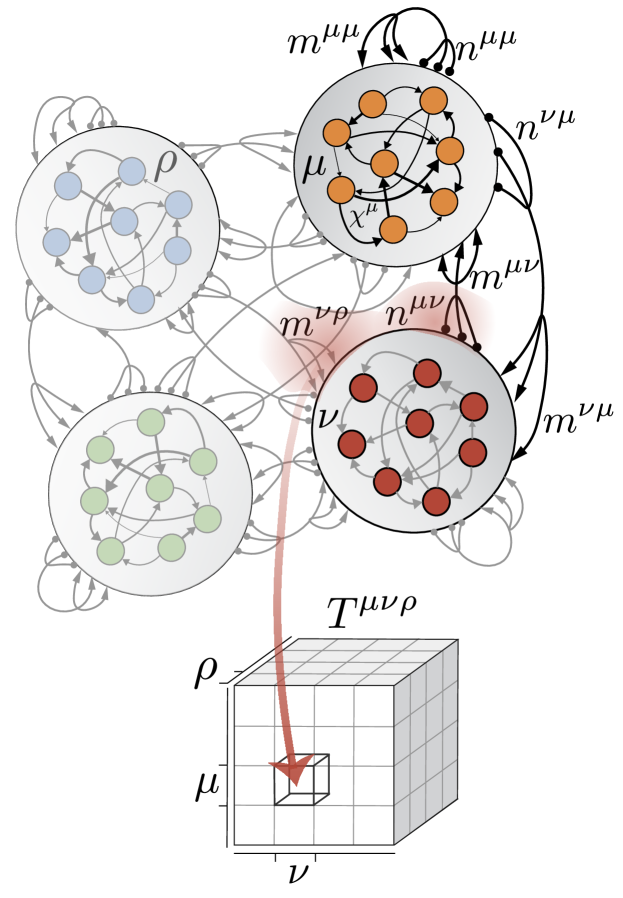
Figure 1: Top: Schematic of the synaptic connectivity model. Different regions, each of which has “random plus rank-one” connectivity, are linked via rank-one matrices representing communication subspaces. In this network of $R=4$ regions, we highlight the rank-one and disordered couplings in region $\mu$, as well as the structured couplings to and from region $\nu$. Rank-one connections are defined through the outer product of vectors $n_{i}^{\mu\nu}$ and $m_{i}^{\nu\rho}$. Bottom: Effective-interaction tensor $T^{\mu\nu\rho}$, which encodes the geometric arrangement of the connectivity patterns and determines the dynamics of region-to-region currents in the mean-field picture. The entry $T^{\mu\nu\rho}$ measures the overlap between $n_{i}^{\mu\nu}$ and $m_{i}^{\nu\rho}$, contracted over the neuron index $i$.

Our approach to generate network behavior between these extremes is rooted in experiments demonstrating that cortical areas interact through so-called communication subspaces. In particular, Semedo et al. [35] found that only a low-dimensional subspace of neural activity in primary visual cortex, V1, shows correlation with activity in V2, and this subspace is distinct from the subspace that captures the most variance of the activity in V1. This can be explained by the synaptic connectivity matrix from V1 to V2 having low-rank structure. In this case, whether activity in V1 is transmitted to V2 depends on the degree of alignment of the activity with the column space of this matrix. That is, an activity-dependent bottleneck limits communication between regions. This study was followed by others demonstrating communication subspaces relevant to visual processing [36], motor control [37, 38], attention [39], audition [22], and brain-wide activity during unstructured behavior [40].

We operationalize this idea by considering couplings of the form

$$J^{\mu\nu}_{ij}=\delta^{\mu\nu}\chi^{\mu}_{ij}+\frac{1}{N}m^{\mu\nu}_{i}n^{\mu\nu}_{j},$$ (4)

where $\left\langle(\chi^{\mu}_{ij})^{2})\right\rangle_{\bm{J}}=(g^{\mu})^{2}/N$. Here, the synaptic connections within region $\mu$ are the sum of random disordered couplings, $\chi^{\mu}_{ij}$, and a rank-one matrix, $m_{i}^{\mu\mu}n_{j}^{\mu\mu}/N$. These terms represent the combination of disorderly and structured recurrent circuitry within brain regions [25]. Meanwhile, to model communication subspaces, the cross-region couplings from region $\nu$ to region $\mu$, for $\mu\neq\nu$, are a rank-one matrix $m_{i}^{\mu\nu}n_{j}^{\mu\nu}/N$ (Fig. 1, top). Note that we study the case where there is no additional disorder in the cross-region connectivity, but we provide DMFT equations incorporating such disorder in Sec.VII (see Eq. 38). The “degree of alignment of the activity with the column space” of a cross-region connectivity matrix, mentioned in the previous paragraph, is given by the inner product of an activity vector $\phi_{i}^{\nu}$ and a connectivity pattern $n^{\mu\nu}_{i}$; these inner products are order parameters in the DMFT.

In this model, there are $2R^{2}$ vector components for each neuron index $i$, namely, ${\{m_{i}^{\mu\nu}\}_{\mu,\nu=1}^{R}\cup\{n_{i}^{\mu\nu}\}_{\mu,\nu=1}^{R}}$. These components are sampled from a zero-mean multivariate Gaussian, i.i.d. across $i$. The second-order statistics of this Gaussian are defined by the tensors

$$T^{\mu\nu\rho} =\left\langle n_{i}^{\mu\nu}m_{i}^{\nu\rho}\right\rangle_{\bm{J}},$$ (5a)

$$U^{\mu\nu\rho} =\left\langle m_{i}^{\mu\nu}m_{i}^{\mu\rho}\right\rangle_{\bm{J}}.$$ (5b)

Specification of the remaining second-order statistics is not required for the mean-field description of the model. However, to sample the vectors defining the low-rank part of the couplings, we must specify $\left\langle n_{i}^{\mu\nu}n_{i}^{\rho\nu}\right\rangle_{\bm{J}}$. We set this proportional to $\delta^{\mu\rho}$ with a positive scale factor large enough so that the full covariance matrix is positive-definite. This scale-factor degree of freedom allows any pair of tensors $T^{\mu\nu\rho}$ and $U^{\mu\nu\rho}$, the latter being symmetric and positive-semidefinite in $(\nu,\rho)$ for all $\mu$, to define a valid distribution over couplings.

As $N\rightarrow\infty$, these tensors are equivalently given by inner products between vectors,

$$T^{\mu\nu\rho} =\frac{1}{N}\sum_{i}{n_{i}^{\mu\nu}m_{i}^{\nu\rho}},$$ (6a)

$$U^{\mu\nu\rho} =\frac{1}{N}\sum_{i}{m_{i}^{\mu\nu}m_{i}^{\mu\rho}}.$$ (6b)

Hence, $T^{\mu\nu\rho}$ and $U^{\mu\nu\rho}$ represent the geometric arrangement of structured low-rank connectivity patterns (Fig. 1, bottom) .

This connectivity allows selective communication of activity between regions in a manner controlled by the geometry encoded in $T^{\mu\nu\rho}$. We first explain this heuristically. If $\phi^{\nu}_{i}$ is an activity pattern in region $\nu$, the activity communicated to region $\mu$ is proportional to the projection $\sum_{i}{n}^{\mu\nu}_{i}\phi^{\nu}_{i}/N$. For a generic pattern $\phi^{\nu}_{i}$ (e.g., induced by the disordered connectivity $\chi^{\nu}_{ij}$), this projection is of order $1/\sqrt{N}$, and thus vanishes for $N\rightarrow\infty$. However, if $\phi_{i}^{\nu}$ has a component along $n_{i}^{\mu\nu}$, this projection is order-one. For this to be the case, there must be a region $\rho$ such that $m^{\nu\rho}_{i}$, which delivers input to region $\nu$, has a component along $n_{i}^{\mu\nu}$. This component is $T^{\mu\nu\rho}$. It follows from this argument that high-dimensional chaotic activity is unable to propagate between regions as $N\rightarrow\infty$.

III Spectral analysis

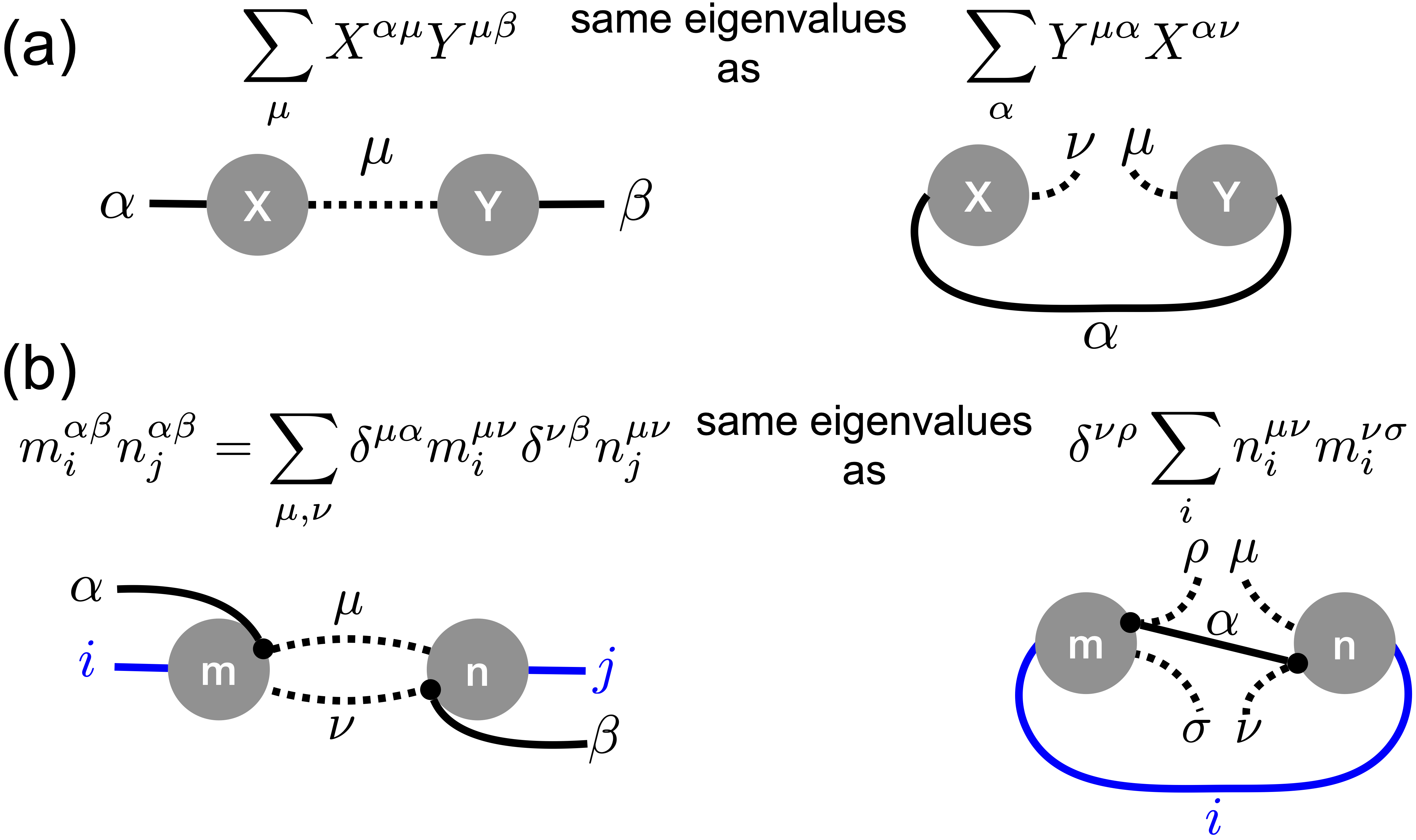
Figure 2: Tensor diagrams illustrating the relationships between (a) matrices $\bm{X}\bm{Y}$ and $\bm{Y}\bm{X}$, and (b) the matrices with more complicated indices relevant to Sec. III. In both (a) and (b), the tensors on the left and right have the same eigenvalues, up to zeros, with respect to the left-right bipartition of the indices. Dangling legs are indices of the output tensor, connected legs are summed over, and $\bullet$ is the Kronecker delta. Dashed lines are summed over on the left and split open on the right; solid lines are dangling on the left and joined on the right.

Before proceeding to the mean-field analysis, we describe the spectrum of $J^{\mu\nu}_{ij}$, which controls the linearized dynamics about the trivial fixed point, $x^{\mu}_{i}=0$. Rather than as a fourth-order tensor, $J^{\mu\nu}_{ij}$ can be interpreted as an $RN$-by-$RN$ matrix with respect to the two “superindices” $(\mu,i)$ and $(\nu,j)$. In other words, the multiregion network can be interpreted as a single large network. This $RN$-by-$RN$ matrix has a bulk spectrum resulting from the random matrices $\chi_{ij}^{\mu}$, whose density in the complex plane, for $N\rightarrow\infty$, is a superposition of $R$ uniform disks of radii $g^{\mu}$.

We denote the low-rank part of the connectivity by ${L^{\mu\nu}_{ij}=m^{\mu\nu}_{i}n^{\mu\nu}_{j}/N}$. This term has up to $R^{2}$ nonzero eigenvalues, which do not interact with the bulk as $N\rightarrow\infty$; they either are outliers or are swallowed by the bulk. To determine these eigenvalues, we seek an $R^{2}$-by-$R^{2}$ matrix whose spectrum coincides with that of $L^{\mu\nu}_{ij}$ as $N\rightarrow\infty$. Such a matrix can be found using the property that the matrices $\bm{X}\bm{Y}$ and $\bm{Y}\bm{X}$ have the same spectra up to zeros (Fig. 2(a)). First, we express the low-rank component as a product of matrices,

$$L^{\alpha\beta}_{ij}=\sum_{\mu,\nu}\frac{\delta^{\mu\alpha}m_{i}^{\mu\nu}}{\sqrt{N}}\frac{\delta^{\nu\beta}n_{j}^{\mu\nu}}{\sqrt{N}},$$ (7)

contracting over the superindex $(\mu,\nu)$ to form a matrix with superindices $(\alpha,i)$ and $(\beta,j)$. The same eigenvalues, up to zeros, are obtained by contracting instead over the superindex $(\alpha,i)=(\beta,j)$, resulting in a matrix with superindices $(\mu,\nu)$ and $(\rho,\sigma)$. This $R^{2}$-by-$R^{2}$ matrix is given by

$$\hat{T}^{\mu\nu,\rho\sigma} =\delta^{\nu\rho}\frac{1}{N}\sum_{i}n_{i}^{\mu\nu}m_{i}^{\nu\rho}$$

$$=\delta^{\nu\rho}T^{\mu\nu\sigma},$$ (8)

where the limit $N\rightarrow\infty$ was taken in the second line. This matrix can also be derived in a single step using a tensor diagram (Fig. 2(b)).

When all eigenvalues of this matrix and the bulk have real parts less than unity, the trivial fixed point of the network is stable, leading to quiescent behavior. If any eigenvalue exceeds this threshold, the network exhibits nontrivial activity described by the DMFT.

IV Dynamical mean-field theory (DMFT)

In the mean-field description of the network, the order parameters comprise the $R$ region-specific two-point functions,

$$\Delta^{\mu}(t,t^{\prime}) =\left\langle x^{\mu}_{i}(t)x^{\mu}_{i}(t^{\prime})\right\rangle_{\bm{J}},$$ (9a)

$$C^{\mu}(t,t^{\prime}) =\left\langle\phi^{\mu}_{i}(t)\phi^{\mu}_{i}(t^{\prime})\right\rangle_{\bm{J}},$$ (9b)

together with $R^{2}$ additional parameters describing pairwise communication between regions,

$$S^{\mu\nu}(t)=\int_{-\infty}^{t}dt^{\prime}e^{-(t-t^{\prime})}\left\langle n^{\mu\nu}_{i}\phi_{i}^{\nu}(t^{\prime})\right\rangle_{\bm{J}},$$ (10)

which is the activity in region $\nu$ that gets communicated to region $\mu$ (after being low-pass filtered). We refer to these variables as currents, borrowing the terminology of Perich et al. [9]. In the mean-field picture, these currents interact according to

$$(1+\partial_{t})S^{\mu\nu}(t) =H^{\mu\nu}(t),\text{ where}$$ (11a)

$$H^{\mu\nu}(t) =\psi^{\nu}(t)\sum_{\rho}{T}^{\mu\nu\rho}S^{\nu\rho}(t),$$ (11b)

which is a matrix dynamics shaped by a third-order tensor. Here, $\psi^{\nu}(t)=\left\langle\phi^{\prime}(x^{\nu}_{i}(t))\right\rangle_{\bm{J}}$ is the average gain of neurons in region $\nu$ at time $t$. Due to the Gaussianity of the preactivations, this can be expressed as $\psi^{\nu}(t)=\psi(\Delta^{\nu}(t,t))$ where

$$\psi(\Delta)=\left\langle\phi^{\prime}(x)\right\rangle_{x},\>\>\>x\sim\mathcal{N}(0,\Delta).$$ (12)

Once $\Delta^{\mu}(t,t)$ has been determined, the dynamics of the currents are given by Eq. 11. Squaring both sides of the network dynamics, Eq. 1, and doing a disorder average gives a dynamic equation for $\Delta^{\mu}(t,t^{\prime})$,

$$(1+\partial_{t})(1+\partial_{t^{\prime}})\Delta^{\mu}(t,t^{\prime})=(g^{\mu})^{2}C^{\mu}(t,t^{\prime})\\ +\sum_{\nu,\rho}U^{\mu\nu\rho}H^{\mu\nu}(t)H^{\mu\rho}(t^{\prime}).$$ (13)

These DMFT equations are closed by expressing $C^{\mu}(t,t^{\prime})$ in terms of $\Delta^{\mu}(t,t^{\prime})$. Again noting the Gaussianity of the preactivations, we have ${C^{\mu}(t,t^{\prime})=C(\Delta(t,t^{\prime}),\Delta(t,t),\Delta(t^{\prime},t^{\prime}))}$, where

$$C(\Delta_{12},\Delta_{11},\Delta_{22})=\left\langle\phi(x_{1})\phi(x_{2})\right\rangle_{x_{1},x_{2}},\\ \left(\begin{array}[]{c}x_{1}\\ x_{2}\end{array}\right)\sim\mathcal{N}\left(\left(\begin{array}[]{c}0\\ 0\end{array}\right),\left(\begin{array}[]{cc}\Delta_{11}&\Delta_{12}\\ \Delta_{12}&\Delta_{22}\end{array}\right)\right).$$ (14)

In the case of the error-function nonlinearity, the Gaussian integrals in Eqs. 12 and 14 can be evaluated analytically to give

$$\psi(\Delta)=\frac{1}{\sqrt{1+{\pi\Delta}/{2}}},$$ (15a)

$$C(\Delta_{12},\Delta_{11},\Delta_{22})$$ (15b)

$$\hskip 22.0pt=\frac{2}{\pi}\text{arctan}\frac{\Delta_{12}}{\sqrt{\left(\Delta_{11}+{2}/{\pi}\right)\left(\Delta_{22}+{2}/{\pi}\right)}}.$$

Eqs. 11–14 comprise a set of deterministic, causal dynamic equations for the $R$ region-specific two-point functions and $R^{2}$ currents. In general, these equations must be solved via numerical integration on a two-dimensional grid (e.g., see [42]). This can be avoided in situations without disorder or with time-translation invariance, both of which we will consider.

For time-independent gains ${\psi^{\nu}(t)=\text{const.}}$ (e.g., at the trivial fixed point), the currents interact via linear dynamics. Note that $\hat{T}^{\mu\nu,\rho\sigma}$, defined in Eq. 8, is the $R^{2}$-by-$R^{2}$ matrix that governs these linear dynamics, i.e.,

$$(1+\partial_{t})S^{\mu\nu}(t)\propto\sum_{\rho,\sigma}\hat{T}^{\mu\nu,\rho\sigma}S^{\rho\sigma}(t).$$ (16)

For this reason, we expect the spectrum of $\hat{T}^{\mu\nu,\rho\sigma}$ to shape the full dynamics of the currents even in the nonlinear case, in analogy with other scenarios where a local linear instability is informative of global nonlinear behavior [43, 44].

Finally, throughout the rest of the paper, we assume $U^{\mu\nu\rho}=\delta^{\nu\rho}$ for all $\mu$, and focus on the role of $T^{\mu\nu\rho}$. Geometrically, this means that inputs from other regions into region $\mu$ are organized in orthogonal subspaces in region $\mu$.

V Symmetric effective interactions

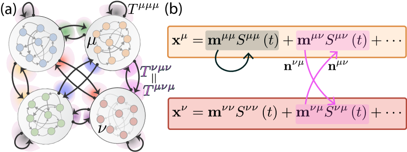
Figure 3: (a) Restriction to the effective-interaction tensor $T^{\mu\nu\rho}$ corresponding to enforcing symmetry. This constraint sets $T^{\mu\nu\rho}=\delta^{\mu\rho}c^{\mu\nu}$, where $c^{\mu\nu}$ is a symmetric matrix. Nonzero overlaps between connectivity patterns are indicated by colored auras, with equal colors indicating equal overlaps. In this scenario with $R=4$ regions, the connectivity has 10 independent parameters: 4 for direct and 6 for indirect effective self-interactions. (b) Illustration of subspace-based routing in the case of symmetric effective interactions. When the activity subspace defined by the span of ${m}_{i}^{\mu\mu}$ in region $\mu$ is excited, bidirectional communication between regions $\mu$ and $\nu$ is suppressed, and vice versa, due to the nonlinear dynamics of the network.

We first make a common assumption in the study of many-body dynamics, namely, that the interactions are symmetric. Enforcing symmetry in this system is nontrivial, however, because the effective interactions are a third-order tensor $T^{\mu\nu\rho}$. As per the above discussion, a natural choice is to impose symmetry on the matrix $\hat{T}^{\mu\nu,\rho\sigma}$, i.e., $\hat{T}^{\mu\nu,\rho\sigma}=\hat{T}^{\rho\sigma,\mu\nu}$. This constraint reduces the number of free parameters from $\mathcal{O}(R^{3})$ to $\mathcal{O}(R^{2})$ by requiring

$$T^{\mu\nu\rho} =\delta^{\mu\rho}c^{\mu\nu},\text{ where }$$ (17a)

$$c^{\mu\nu} =c^{\nu\mu}.$$ (17b)

In contrast, for standard coupling matrices, imposing symmetry does not reduce the scaling of the number of parameters. Note that, even with this constraint, the high-dimensional couplings $J^{\mu\nu}_{ij}$ are not symmetric, both because the matrices $\chi^{\mu}_{ij}$ are asymmetric, and because sampling the vectors $m^{\mu\nu}_{i}$ and $n^{\mu\nu}_{i}$ results in ${m^{\mu\nu}_{i}n^{\mu\nu}_{j}\neq m^{\nu\mu}_{j}n^{\nu\mu}_{i}}$.

The presence of $\delta^{\mu\rho}$ in Eq. 17a implies that each region $\mu$ either interacts directly with itself ($\mu=\nu$) or does so indirectly through an intermediate region, $\nu$ ($\mu\neq\nu$). Moreover, the symmetry of $c^{\mu\nu}$, Eq. 17b, implies that the coupling through which region $\mu$ interacts with itself via region $\nu$ is equivalent to that for region $\nu$ interacting with itself via region $\mu$. In terms of the geometric arrangement of connectivity patterns, these constraints imply that within region $\mu$, the vectors $n^{\mu\mu}_{i}$ and $m^{\mu\mu}_{i}$ have nontrivial overlap; similarly, the vectors $n^{\mu\nu}_{i}$ and $m^{\nu\mu}_{i}$, which define how activity is extracted from region $\nu$ and provided to region $\mu$, also have nontrivial overlap. This latter overlap is the same when $\mu$ and $\nu$ are switched in accordance with the symmetry of $c^{\mu\nu}$. All other overlaps are zero. This geometric arrangement of connectivity patterns underpins the dynamics of subspace-based signal routing, with orthogonality between pairs of vectors replacing the traditional notion of connectivity sparsity. This is illustrated in Fig. 3(a).

To make analytical progress, we further constrain $c^{\mu\nu}$ to have a “rank-one plus diagonal” form with only $\mathcal{O}(R)$ parameters,

$$c^{\mu\nu}=u^{\mu}u^{\nu}+\delta^{\mu\nu}h^{\mu},$$ (18)

where $u^{\mu}$ and $h^{\mu}$ are arbitrary vectors. The expressivity of this parameterization of a symmetric matrix is well known from the factor-analysis model in statistics [45]. This parameterization provides a minimal example in which one has independent control over the strength of direct versus indirect self-connectivity, which are captured by the quantities

$$a^{\mu} =(u^{\mu})^{2}+h^{\mu},\text{ and}$$ (19a)

$$b^{\mu} =(u^{\mu})^{2},$$ (19b)

respectively. Finally, the $R^{2}$ eigenvalues of $\hat{T}^{\mu\nu,\rho\sigma}$ are $a^{\mu}$ for all $\mu$ and $\pm\sqrt{|b^{\mu}b^{\nu}|}$ for all pairs $\mu\neq\nu$. We will assume that, for each $\mu$, ${\text{max}(a^{\mu},b^{\mu})>1}$.

V.1 Disorder-free case

The lack of disorder simplifies the DMFT because the variance of neurons is due solely to the currents. Mathematically, setting $g^{\mu}=0$ implies that the two-point function dynamics, Eq. 13, can be integrated to give $\Delta^{\mu}(t,t)=\sum_{\nu}(S^{\mu\nu}(t))^{2}$. Generically, symmetric interactions lead to fixed points, and this is the case here. Upon setting $g^{\mu}$ and the time-derivative to zero in the DMFT equations (Eqs. 11–14) and further specializing to the parameterization of $T^{\mu\nu\rho}$ given above, fixed points $S^{\mu\nu}_{0}$ of the disorder-free current dynamics satisfy

$$S_{0}^{\mu\nu} =\psi_{0}^{\nu}(u^{\mu}u^{\nu}+\delta^{\mu\nu}h^{\nu})S_{0}^{\nu\mu},$$ (20a)

$$\psi^{\nu}_{0} =\psi(A^{\nu}),$$ (20b)

$$A^{\nu} =\sum_{\rho}{(S_{0}^{\nu\rho})^{2}},$$ (20c)

where we introduce the variable $A^{\mu}$ to represent the squared $L^{2}$-norm of row $\mu$ of the current matrix. In the disorder-free case, these norms are equivalent to the variance of neurons in region $\mu$, $A^{\mu}=\Delta^{\mu}(0)$.

Solving these equations allows us to determine a broad class of stable and unstable fixed points, including the stable fixed points encountered in simulations. Solutions in this class have the following structure, detailed below. Each region $\mu$ can either be a generator of current, $S_{0}^{\mu\mu}\neq 0$, blocking signal transmission; or lack self-excitation, $S_{0}^{\mu\mu}=0$, allowing signal transmission and participating in a network-level set of fixed points. We refer to these region-specific behaviors as non-routing and routing modes, respectively, and define $\mathcal{S}_{\text{route}}\subseteq\{1,\ldots,R\}$ to be the subset of regions in routing mode. Examples of these cases, which exemplify the tension between signal generation and transmission, are shown in Fig. 4.

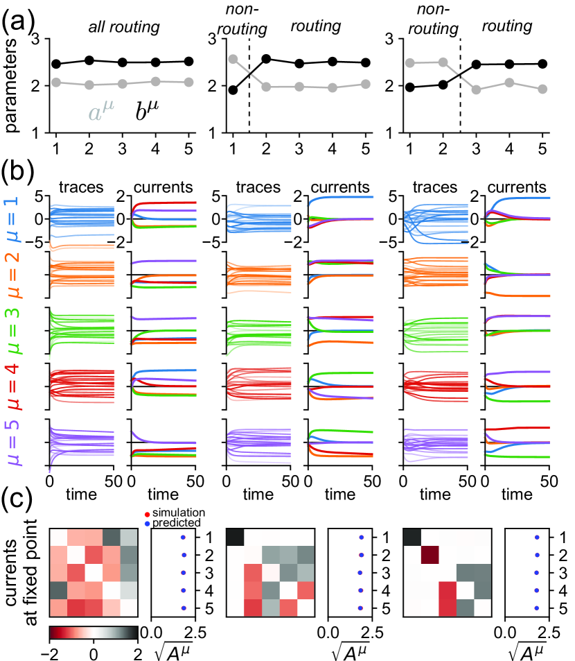
Figure 4: Structure of fixed points in networks with symmetric effective interactions. The same information for three different cases is shown on the left, center and right. (a) Values of $a^{\mu}$ and $b^{\mu}$ in the $R=5$ regions. (b) Dynamics of sampled neurons (left) and of incoming currents (right) in large simulations for each region. (c) Visualization of the steady-state current matrix $S^{\mu\nu}_{0}$ (left) and of the $L^{2}$-norms of the rows of this matrix (right). We show row-norms from the simulations (red dots) alongside analytical predictions (blue dot). In the leftmost plots, all regions are in non-routing mode. In the middle plots, region 1 is in non-routing mode and regions 2–4 are in routing mode. In the rightmost plots, regions 1 and 2 are in non-routing mode and regions 3–5 are in routing mode.

Quantitatively, for a region $\mu$ in non-routing mode,

$$\psi_{0}^{\mu} =\frac{1}{a^{\mu}},$$ (21a)

$$(S_{0}^{\mu\mu})^{2} =A^{\mu},$$ (21b)

$$S_{0}^{\mu\nu} =S_{0}^{\nu\mu}=0\text{ for all }\nu\neq\mu;$$ (21c)

and, for a region $\mu$ in routing mode,

$$\psi_{0}^{\mu} =\frac{1}{b^{\mu}},$$ (22a)

$$S_{0}^{\mu\mu} =0,$$ (22b)

$$S_{0}^{\mu\nu}u^{\nu} =S_{0}^{\nu\mu}u^{\mu}\text{ for all }\nu\in\mathcal{S}_{\text{route}}\setminus\{\mu\}.$$ (22c)

Additionally, for the subset of regions in routing mode, there are group constraints on the squared $L^{2}$-norms of the rows of $S_{0}^{\mu\nu}$,

$$\sum_{\nu\in\mathcal{S}_{\text{route}}\setminus\{\mu\}}(S_{0}^{\mu\nu})^{2}=A^{\mu}\text{ for all {\hbox{\mu\in\mathcal{S}_\text{route}}}}.$$ (23)

Based on Eqs. 21 and  22, the squared $L^{2}$-norm of the currents received by region $\mu$ takes one of two possible values, depending on whether $\mu$ is in routing or non-routing mode:

$$A^{\mu}=\begin{cases}\psi^{-1}\left(\frac{1}{b^{\mu}}\right)&\mu\in\mathcal{S}_{\text{route}}\\ \psi^{-1}\left(\frac{1}{a^{\mu}}\right)&\text{otherwise}.\end{cases}$$ (24)

Here, $\psi^{-1}(1/x)$ is a monotonically increasing function of $x$, so the norm of row $\mu$ increases with $a^{\mu}$ or $b^{\mu}$. For the error-function nonlinearity, ${\psi^{-1}(1/x)=2(x^{2}-1)/\pi}$.

Finally, despite the symmetry of the effective interactions, $S^{\mu}_{0}$ itself is not symmetric. Instead, $S^{\mu\nu}_{0}$ has a generalized symmetry property, namely, that both $S^{\mu\nu}_{0}u^{\nu}$ and $S^{\mu\nu}_{0}/u^{\mu}$ are symmetric.

V.2 Stability

There are $2^{R}$ ways to assign routing and non-routing modes to regions. Which of these configurations are stable? We will show that stable states are characterized by region $\mu$ being in routing mode if $a^{\mu}<b^{\mu}$ and in non-routing mode if $a^{\mu}>b^{\mu}$. The degree of intrinsic recurrent activity within a region therefore acts as a gate, controlling whether signals from other regions are transmitted.

The tensorial form of the Jacobian makes it difficult to assess stability by calculating its spectrum analytically, so we instead consider a first-order perturbation $\sigma^{\mu\nu}\left(t\right)$ about a fixed point $S_{0}^{\mu\nu}$ and define a “local energy,”

$$E[\bm{\sigma}]=\frac{1}{2}\sum_{\mu,\nu}\left(\frac{\sigma^{\mu\nu}}{u^{\mu}}\right)^{2},$$ (25)

where the factor $1/u^{\mu}$ is inspired by the generalized symmetry property. We will show that $\partial_{t}E\leq 0$ for all $\sigma^{\mu\nu}$ when $S^{\mu\nu}_{0}$ is in a configuration claimed to be stable. Computing the time derivative and subsequently replacing $\sigma^{\mu\nu}\rightarrow u^{\mu}\sigma^{\mu\nu}$ gives $\partial_{t}E=\sum_{\nu}e^{\nu}$, where

$$e^{\nu}= -\sum_{\mu}(\sigma^{\mu\nu})^{2}+b^{\nu}\psi_{0}^{\nu}\sum_{\mu}\sigma^{\nu\mu}\sigma^{\mu\nu}$$

$$+2b^{\nu}\psi^{\prime\nu}_{0}\Big{(}\sum_{\mu}S_{0}^{\nu\mu}\sigma^{\mu\nu}\Big{)}\Big{(}\sum_{\rho}S_{0}^{\nu\rho}\sigma^{\nu\rho}\Big{)}$$

$$+h^{\nu}(\sigma^{\nu\nu})^{2}\left(\psi_{0}^{\nu}+2\psi^{\prime\nu}_{0}(S_{0}^{\nu\nu})^{2}\right),$$ (26)

where $\psi^{\nu}_{0}=\psi(A^{\nu})$ and $\psi^{\prime\nu}_{0}=\psi^{\prime}(A^{\nu})$. We perform a symmetric-antisymmetric decomposition, ${\sigma^{\mu\nu}=\alpha^{\mu\nu}+\beta^{\mu\nu}}$, where ${\alpha^{\mu\nu}=\alpha^{\nu\mu}}$ and ${\beta^{\mu\nu}=-\beta^{\nu\mu}}$, and discard the term $-2\sum_{\mu}\alpha^{\mu\nu}\beta^{\mu\nu}$, which vanishes under the outer $\nu$ sum. We then have for a region $\nu$ in routing mode

$$e^{\nu}=2b^{\nu}\psi^{\prime\nu}_{0}\Big{(}\sum_{\mu}S_{0}^{\mu\nu}\alpha^{\mu\nu}\Big{)}^{2}+h^{\nu}\psi_{0}^{\nu}(\alpha^{\nu\nu})^{2}\\ -2\sum_{\mu}(\beta^{\mu\nu})^{2}-2b^{\nu}\psi^{\prime\nu}_{0}\Big{(}\sum_{\mu}S_{0}^{\mu\nu}\beta^{\mu\nu}\Big{)}^{2}.$$ (27)

The first term is nonpositive since $\psi^{\prime\nu}_{0}<0$. The second is nonpositive when $h^{\nu}<0$, i.e., $a^{\nu}<b^{\nu}$. The third and fourth terms, involving $\beta^{\mu\nu}$, are net-nonpositive for all $\beta^{\mu\nu}$ if, and only if, ${-{\psi^{\prime}(\Delta)\Delta}/{\psi(\Delta)}\leq 1}$. This quantity varies between 0 to $1/2$ as $\Delta$ varies from zero to infinity, so this holds. Thus, $\partial_{t}E\leq 0$.

For a region $\nu$ in non-routing mode,

$$e^{\nu}=-\left(1-\frac{b^{\nu}}{a^{\nu}}\right)\sum_{\mu\neq\nu}(\alpha^{\mu\nu})^{2}+{2a^{\nu}\psi^{\prime\nu}_{0}(S_{0}^{\nu\nu})^{2}}(\alpha^{\nu\nu})^{2}\\ -\left(1+\frac{b^{\nu}}{a^{\nu}}\right)\sum_{\mu}(\beta^{\mu\nu})^{2}.$$ (28)

The second and third terms are nonpositive, and the first is nonpositive for $a^{\nu}>b^{\nu}$. Thus, when the routing and non-routing modes are chosen according to whether $a^{\mu}$ or $b^{\mu}$ is larger, the resulting state is stable.

Conversely, if there is a routing mode with ${a^{\mu}>b^{\mu}}$, we obtain $\partial_{t}E>0$ by picking $\alpha^{\mu\mu}$ to be nonzero and all other components of $\alpha^{\mu\nu}$ and $\beta^{\mu\nu}$ to be zero. Similarly, if there is a non-routing mode with $a^{\mu}<b^{\mu}$, we obtain $\partial_{t}E>0$ by picking $\alpha^{\mu\nu}$ to be nonzero and orthogonal to $S^{\mu\nu}_{0}$ when contracted over $\nu$, and everything else zero. These choices of $\sigma^{\mu\nu}$ indicate directions along which perturbations grow away from the fixed point. For a region $\mu$ in routing mode, there are directions in which the local energy neither grows nor shrinks, $\partial_{t}E=0$, obtained by $\alpha^{\mu\nu}$ being nonzero and orthogonal to $S^{\mu\nu}_{0}$ when contracted over $\nu$, and everything else zero. We show in Sec. V.4 that such directions correspond to translation along a continuous attractor manifold.

While $\partial_{t}E\leq 0$ rigorously indicates (marginal) stability, $\partial_{t}E>0$ does not necessarily indicate instability; it might reflect transient dynamics en route to a stable state. Nevertheless, we find through numerical diagonalization of the Jacobian that the perturbations with $\partial_{t}E>0$ given above indeed represent unstable directions. An interesting, as yet unanswered question is whether this system, under the symmetry constraint, possesses a global energy function that ensures convergence to fixed points from any initial condition, similar to regular neural networks with coupling symmetry.

Before we introduce disorder into the model, we highlight how the method for routing neural signals used here differs from traditional approaches. Traditional approaches typically relied on manipulating individual neurons or synapses through neuromodulation, inhibition, or gain modulation. In contrast, our approach bases the transmission of signals between regions on the geometry of neural population activity. Specifically, instead of significantly reducing $\psi_{0}^{\mu}$ to switch a region $\mu$ to a non-routing mode–akin to gain control–our model leverages the interaction between connectivity geometry and nonlinear recurrent dynamics. This interaction aligns neural activity with subspaces that allow or prevent cross-region communication. This is illustrated in Fig. 3(b). Thus, our model offers a new perspective on routing in neural circuits, emphasizing the excitation of subspaces sculpted by the structure of connectivity and network dynamics.

V.3 Effect of disorder

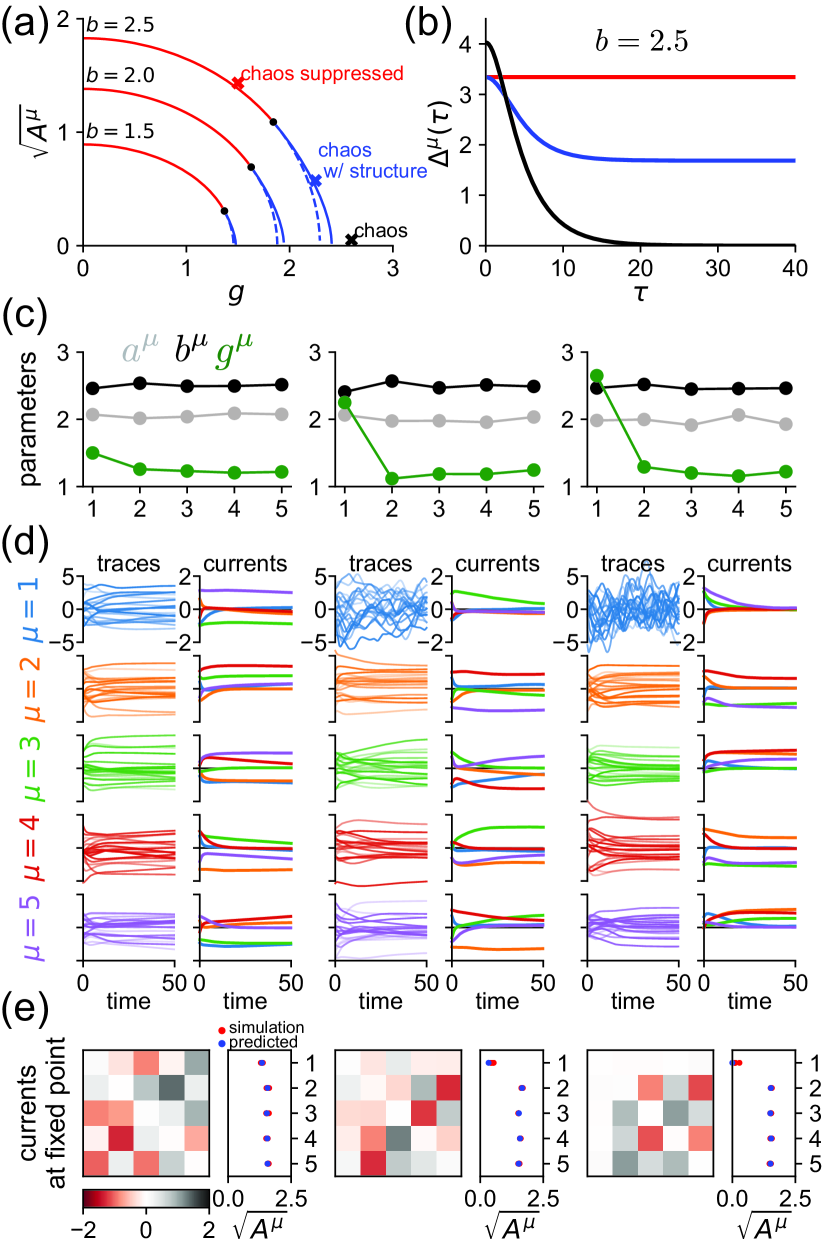
Figure 5: Structure of activity in networks with disorder and symmetric effective interactions among regions. (a) Relationship between $A^{\mu}$ and $g^{\mu}$ for various values of $b^{\mu}$ in the DMFT. (b) Solutions for the two-point function $\Delta^{\mu}(\tau)$ for the parameter values indicated by the markers in (a). (c–e) are the same as (a–c) in Fig. 4, but with disorder, whose levels are shown in (a). All regions have $g^{\mu}>1$, so regions produce chaotic fluctuations unless tamed by current-based activity. In the leftmost plots, chaos is suppressed in all regions, and all regions are in routing mode. In the middle plots, all regions are in routing mode, and chaotic fluctuations exist alongside the structured current-based activity in region 1. In the rightmost plots, region 1 is in disorder-dominated non-routing mode, and regions 2–5 are in routing mode.

In this section, we introduce disorder into the model by allowing nonzero $g^{\mu}$, potentially leading to high-dimensional chaotic fluctuations. Such fluctuations can disrupt signal transmission between regions. In particular, chaos scrambles neural signals, preventing coherent communication. This is comparable to the structure-dominated non-routing mode discussed above, where structured within-region activity impedes signal flow. Both types of non-routing behaviors exemplify the underlying tension between signal generation and transmission.

The symmetric structure of the effective-interaction tensor implies that, even with disorder, the currents converge to fixed points, $S^{\mu\nu}_{0}$. Due to the possibility of coexisting high-dimensional chaotic fluctuations, $\Delta^{\mu}(t,t^{\prime})$ can depend on time. We seek stationary solutions, $\Delta(t,t^{\prime})=\Delta(\tau)$ where $\tau=t-t^{\prime}$, in which case the DMFT equations become

$$S_{0}^{\mu\nu} =\psi^{\nu}_{0}(u^{\mu}u^{\nu}+\delta^{\mu\nu}h^{\nu})S_{0}^{\nu\mu},$$ (29a)

$$\psi_{0}^{\nu} =\psi(\Delta^{\nu}(0)),$$ (29b)

$$\partial_{\tau}^{2}\Delta^{\mu}(\tau) =-\partial_{\Delta^{\mu}}V^{\mu}(\Delta^{\mu};A^{\mu}),$$ (29c)

$$V^{\mu}(\Delta^{\mu};A^{\mu}) =-\frac{(\Delta^{\mu})^{2}}{2}$$

$$\hskip 11.99998pt+(g^{\mu})^{2}\Phi(\Delta^{\mu},\Delta^{\mu}(0))+A^{\mu}\Delta^{\mu},$$ (29d)

$$A^{\mu} =\sum_{\nu}(S_{0}^{\mu\nu})^{2},$$ (29e)

where we replaced ${(1+\partial_{t})(1+\partial_{t^{\prime}})\rightarrow 1-\partial_{\tau}^{2}}$ in Eq. 13, then integrated its rhs with respect to $\Delta^{\mu}(\tau)$. To obtain $\Phi(\Delta_{12},\Delta_{11})$, we first define $C(\Delta_{12},\Delta_{11})$ by setting $\Delta_{11}=\Delta_{12}$ in Eq. 15b, then integrate with respect to $\Delta_{12}$.

These equations generalize Eq. 20 to the case where the squared $L^{2}$-norms of the rows of the current matrix differ from the equal-time two-point functions, ${A^{\mu}\neq\Delta^{\mu}(0)}$, due to chaotic fluctuations contributing to the variance of activity in addition to the currents. As in Sompolinsky et al. [33], $\Delta^{\mu}(\tau)$ acts like a Newtonian particle in a Mexican-hat potential, $V^{\mu}(\Delta^{\mu};A^{\mu})$. The values of $\psi^{\mu}_{0}$ and thus $\Delta^{\mu}(0)$ are determined by $a^{\mu}$ and $b^{\mu}$ as in the disorder-free case, but $A^{\mu}$ is as yet undetermined. We exchange the dependence of the potential on $A^{\mu}$ for a dependence on the large-$\tau$ value of the two-point function, ${\Delta^{\mu}(\infty)=\lim_{\tau\rightarrow\infty}\Delta^{\mu}(\tau)}$, which satisfies $\partial_{\Delta^{\mu}}V^{\mu}(\Delta^{\mu}(\infty))=0$ because the Newtonian particle must come to rest at the top of a hill to obtain a valid decaying two-point function. This condition can be expressed as

$$A^{\mu}=\Delta^{\mu}(\infty)-(g^{\mu})^{2}C(\Delta^{\mu}(\infty),\Delta^{\mu}(0)).$$ (30)

We use this to express the potential as $V^{\mu}(\Delta^{\mu};\Delta^{\mu}(\infty))$, eliminating the dependence on $A^{\mu}$. Finally, $\Delta^{\mu}(\infty)$ is determined by energy conservation, $V^{\mu}(\Delta^{\mu}(0);\Delta^{\mu}(\infty))=V^{\mu}(\Delta^{\mu}(\infty);\Delta^{\mu}(\infty))$. $A^{\mu}$ can then be found using Eq. 30, shown in Fig. 5(a), and the full form of $\Delta^{\mu}(\tau)$ is given by integrating the Newtonian dynamics, shown in Fig. 5(b). A similar analysis was done by Mastrogiuseppe and Ostojic [25].

Solutions of these equations have the following structure, depicted in Figs. 5(c–e). When $g^{\mu}$ is small, chaotic fluctuations are not present in region $\mu$, so $\Delta^{\mu}(\tau)=\Delta^{\mu}(0)=\Delta^{\mu}(\infty)$. Routing and non-routing modes behave as in the disorder-free case, namely, $\psi^{\mu}=1/a^{\mu}$ or $\psi^{\mu}=1/b^{\mu}$, with the same constraints on the placement of zeros in the current matrix, and with stability determined by whether $a^{\mu}$ or $b^{\mu}$ is larger. This non-chaotic regime exists for $g^{\mu}>1$, reflecting the suppression of chaos by currents emanating from within the region, if in non-routing mode, or from other regions, if in routing mode. Compared to the disorder-free case, $A^{\mu}$ is reduced, implying that disorder hinders currents. As $g^{\mu}$ increases, there is a phase transition to a regime in which chaotic fluctuations coexist with currents, corresponding to $\Delta^{\mu}(\infty)<\Delta^{\mu}(0)$ with $\Delta^{\mu}(\tau)$ decaying. In both of these phases, disorder-induced reductions of $A^{\mu}$ can change the topology of the set of fixed points, as we show in Sec. V.4.

When $g^{\mu}$ becomes sufficiently large, there is a phase transition to a new type of non-routing mode dominated by disorder. In this case, $\Delta^{\mu}(\tau)$ decays from $\Delta^{\mu}(0)>0$ to $\Delta^{\mu}(\infty)=0$, and $A^{\mu}=0$. The values of $\psi_{0}^{\mu}$ and $\Delta^{\mu}(\tau)$ are no longer determined by $a^{\mu}$ and $b^{\mu}$; instead, $\Delta^{\mu}(\tau)$ follows the solution of [33] as if there were no structured connectivity. This phase differs from the structure-dominated non-routing mode, described in the previous section, in that signal transmission from other regions is thwarted by high-dimensional chaotic fluctuations rather than structured self-exciting activity, resulting in $S^{\mu\mu}_{0}=0$. That is, chaotic fluctuations scramble incoming and outgoing signals to the degree that reliable signal transmission is not possible. These disorder-induced phase transitions are decoupled across regions because the low-rank structure of the cross-region connectivity prevents propagation of high-dimensional chaotic fluctuations.

V.4 Dimension and topology of the attractor manifold

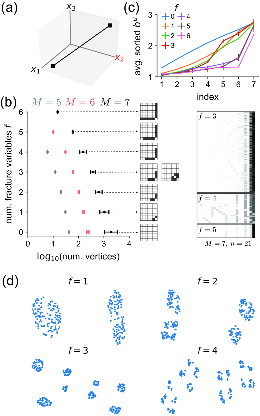
Figure 6: Convex geometry of the attractor manifold in multiregion networks. (a) Cartoon illustration of fracture variables. In a cartoon “feasible region” defined by a line segment, $x_{2}$ is never zero, leading to a binary fracturing of the current-space manifold. (b) Left: Summary of the geometry of the solution polytope, determined by random choices of $\bm{b}$. For each choice, a point is plotted in a plane with axes representing the log-number of vertices and the number of fracture variables, $f$. Different colors indicate different numbers of regions in routing mode, $M$. Center: Configurations of the current submatrix at fixed points for choices of $\bm{b}$ resulting in $f$ fracture variables, with increasing values of $f$ (ascending) and $M=7$. Right: “Barcode” visualization of all vertices of the feasible region, in $\bm{x}$ space, for specific choices of $\bm{b}$. Here, $M=7$, and thus there are $n=21$ variables in the linear program. Barcodes for $f\in\{3,4,5\}$ are displayed (descending). (c) Averaged sorted values of $b^{\mu}$, conditioned on yielding specified numbers of fracture variables $f$. (d) t-SNE visualizations of fixed-point manifolds, in current space, for various numbers of fracture variables $f$ with $M=7$.

By imposing symmetry on the effective-interaction tensor, the multiregion system acts as an attractor network, with the currents (but, if disorder is present, not necessarily neuronal activations) converging to fixed points. These equilibrium states remain unchanged over a timescale significantly longer than that of individual neurons, becoming infinite as $N\rightarrow\infty$. In neuroscience, attractor dynamics have been theoretically and experimentally successful in explaining memory mechanisms involving discrete and continuous variables, as well as in the integration of continuous variables. Models in this category include discrete attractors, such as Hopfield networks [46]; and continuous attractors, such as line [23], ring [47, 48, 49], and toroidal attractors [50, 51]. These various structures are appropriate for different cognitive tasks; for instance, discrete attractors are useful for tasks requiring the retention and recall of specific information, whereas continuous attractors are useful for tasks involving the tracking or integration of ongoing stimuli or movements.

Our analysis thus far focused on the structure of fixed points without considering the dimension and topology of the manifold on which they reside. We now explore the structure of this current-space manifold, which is linearly embedded in neuronal space, through a connection to convex geometry. We demonstrate that the architecture of the multiregion network facilitates a blend of discrete and continuous attractors, potentially useful for tasks that necessitate tracking continuous signals in a context-specific way. Furthermore, the dimension and topology of the manifold can be modified by adjusting the effective interactions, rather than by rewiring the network architecture. We begin by reducing the problem of determining the structure of the current-space manifold to a linear program, then use this linear-program equivalence to describe the manifold’s dimension and topology.

For both the disordered and non-disordered cases, the structure of the current-space manifold is shaped by three constraints on the submatrix of $S^{\mu\nu}_{0}$ restricted to the set of regions $\mathcal{S}_{\text{route}}$ in routing mode: 1) zero on-diagonals; 2) equality constraints on the squared $L^{2}$-norms of rows (involving $A^{\mu}$); and 3) the generalized symmetry property, ${S_{0}^{\mu\nu}u^{\nu}=S_{0}^{\nu\mu}u^{\mu}}$. We encode these constraints as a linear program with a vector of variables $\bm{x}$. These variables correspond to the squared upper-triangular elements of the current submatrix restricted to regions in routing mode,

$$\bm{x}=\{(S^{\mu\nu}_{0})^{2}\>|\>\mu,\nu\in\mathcal{S}_{\text{route}},\>\mu<\nu\}.$$ (31)

Thus, the size of $\bm{x}$ is ${n=M(M-1)/2}$, where $M=|\mathcal{S}_{\text{route}}|$ is the number of regions in routing mode. Crucially, there is a nonnegativity constraint, $x_{k}\geq 0$ for $k\in\{1,\ldots,n\}$, because the variables represent squared quantities.

There are $M$ linear equality constraints that can be expressed as $\bm{C}\bm{x}=\bm{A}$. Here, $\bm{A}$ has components $A^{\mu}$, where $A^{\mu}$ is the required squared $L^{2}$-norm of row $\mu$ of the current submatrix, and $\bm{C}$ is an $M$-by-$n$ constraint matrix. Each element of $\bm{C}$ is set to unity or the ratio $b^{\mu}/b^{\nu}$ if the element corresponds to an upper- or lower-triangular element of the current submatrix, respectively; otherwise the element is set to zero. For concreteness, in the case of $M=5$, symmetric pairs of elements of the current submatrix can be indexed from $1$ through $n=10$ as

$$\begin{pmatrix}\bullet&1&2&3&4\\ 1&\bullet&5&6&7\\ 2&5&\bullet&8&9\\ 3&6&8&\bullet&10\\ 4&7&9&10&\bullet\\ \end{pmatrix},$$ (32)

which gives the constraint matrix

$$\bm{C}=\begin{pmatrix}1&1&1&1&0&0&0&0&0&0\\ \frac{b_{2}}{b_{1}}&0&0&0&1&1&1&0&0&0\\ 0&\frac{b_{3}}{b_{1}}&0&0&\frac{b_{3}}{b_{2}}&0&0&1&1&0\\ 0&0&\frac{b_{4}}{b_{1}}&0&0&\frac{b_{4}}{b_{2}}&0&\frac{b_{4}}{b_{3}}&0&1\\ 0&0&0&\frac{b_{5}}{b_{1}}&0&0&\frac{b_{5}}{b_{2}}&0&\frac{b_{5}}{b_{3}}&\frac{b_{5}}{b_{4}}\\ \end{pmatrix}.$$ (33)

The solution set of this linear program, called the feasible region, is a convex polytope. The dimension $d$ of the feasible region is, barring fine tuning, the number of variables minus the number of constraints,

$$d=n-M=\frac{M(M-3)}{2}.$$ (34)

This is also the dimension of the current-space manifold. Thus, for $M\geq 4$, the manifold is continuous with dimension $d\geq 2$. For $M=3$, the manifold reduces to a zero-dimensional point set. For $M=2$, or for a sufficiently nonuniform constraint vector $\bm{A}$, the linear program is infeasible (i.e., has no solutions). In this case, the assumptions of the linear-program formulation are violated and we must return to the fixed-point equations. We revisit this momentarily.

To characterize the topology of the current-space manifold, we first observe that, for a given point $\bm{x}$ on the feasible region, there are $2^{n}$ corresponding points in current space. This multiplicity arises from the different ways one can choose the signs of the currents. The connectedness, or lack thereof, of current space hinges on whether $x_{k}=0$ for each $k\in\{1,\ldots,n\}$ is included in the feasible region. If included, positive and negative current-space branches connect; otherwise, a binary fracture of the manifold is induced. We refer to variables $x_{k}$ that never take on zero as fracture variables and denote their number by $f$. This is visualized in Fig. 6(a). Each fracture variable contributes one binary split to the manifold, resulting in $2^{f}$ connected components. Zeros in components of $\bm{x}$ occur only at vertices of the feasible region, so to identify all fracture variables, it suffices to enumerate all vertices. This can be done using the double-description method of Motzkin [52, 53]. Alternatively, to determine if $x_{k}$ is a fracture variable, one could set $x_{k}=0$ and check if the resulting linear program in $n-1$ variables is feasible using the efficient simplex algorithm.

To generate many realizations of this linear program, we repeatedly do the following. We first pick a vector $\bm{b}$ by sampling its components $b^{\mu}$ uniformly over $1\leq b^{\mu}\leq 3$ and sort the components in ascending order for visualization purposes. We then set $A^{\mu}=\psi^{-1}(1/b^{\mu})$ for each $\mu$, effectively assuming the disorder-free case with all regions in routing mode (Eq. 24). We then use the double-description algorithm to identify all verities. We summarize the results of this analysis by plotting the number of fracture variables $f$ against the log-number of vertices for many realizations of the linear program with $M\in\{5,6,7\}$ (Fig. 6(b), left). The typical number of vertices grows exponentially in $M$. $f$ is negatively correlated with the number of vertices and is at most $M-1$. With the exception of $f=3$, we find that, for a given choice of $\bm{b}$, all fracture variables correspond to the incoming and outgoing currents for a single region, specifically, the one with largest $b^{\mu}$ (Fig. 6(b), center). For $f=3$, there is an additional configuration where the variables corresponding to all three currents between the three regions with the largest values of $b^{\mu}$ are fracture variables. We visualized all $n=21$ vertices for example realizations of the linear program with $M=7$ and $f\in\{3,4,5\}$ (Fig. 6(b), right). Choices of $\bm{b}$ that lead to larger numbers of fracture variables tend to have nonuniform components (Fig. 6(c)).

We confirmed that the topology predicted by fracture variables matches that of the current-space manifold. For various samples of $\bm{b}$, we evolved the disorder-free DMFT equations with a large number of initial conditions until convergence to fixed points. We then applied t-SNE nonlinear dimensionality reduction to the collection of fixed points [54]. As expected, the number of distinct clusters was $2^{f}$ in all cases, as visualized in Fig. 6(d). Each cluster has some spread corresponding to the continuous dimensions of variation on the manifold.

If ${M=2}$, or if the values of $b^{\mu}$ are highly nonuniform, the linear program is infeasible. Because the trivial fixed point is unstable, there must be at least one stable, nontrivial fixed point in this case that violates the form assumed to parameterize the linear program. We find that this exceptional fixed point is unique up to sign flips and has all current submatrix elements set to zero except for the incoming and outgoing currents in the region with the highest value of $b^{\mu}$. If this maximal value is $b^{M}$, this exceptional fixed point can be found by first finding $\psi^{M}_{0}$ by solving

$$\psi^{M}_{0}=\psi\left(\sum_{\mu=1}^{M-1}\frac{\psi^{-1}\left(\frac{1}{b^{\mu}b^{M}\psi_{0}^{M}}\right)}{b^{\mu}b^{M}(\psi_{0}^{M})^{2}}\right),$$ (35)

from which $S_{0}^{\mu M}$ and $S_{0}^{M\mu}$ follow. We find that this fixed point becomes stable when the linear program becomes infeasible.

The dimension and topology of the current-space manifold are determined by the number of regions in routing mode and the values of $A^{\mu}$, respectively. Modifications to these quantities can be achieved by adjusting the parameters $a^{\mu}$, $b^{\mu}$, and $g^{\mu}$. Therefore, dynamically altering the strengths of interactions (for instance, through neuromodulation) offers a method to maintain an attractor manifold with a variable dimension and number of connected components, without the need to construct a completely new network architecture. This adaptability could be advantageous for responding to various cognitive tasks or environmental conditions, where the computational demands on the attractor system may change rapidly and significantly.

VI Asymmetric effective interactions

So far, we have restricted our analysis to effective interactions with a symmetry constraint. We now lift this constraint, allowing the effective-interaction tensor to have arbitrary elements. In this case, the current dynamics need not be dominated by fixed points. To analyze the dependence of the current dynamics on the geometric structure of the connectivity, we turn to the spectrum of $\hat{T}^{\mu\nu,\rho\sigma}$. When this matrix has a real leading eigenvalue (where “leading” refers to having greatest real part), the current dynamics tend to converge to fixed points. When there is instead a complex-conjugate pair of leading eigenvalues, particularly with large imaginary part, the currents typically show limit cycles. We have not found chaotic attractors in the currents.

We characterize the relationships between the current dynamics, within-region chaotic fluctuations, and the leading eigenvalue of $\hat{T}^{\mu\nu,\rho\sigma}$ through the following analysis. We consider networks of $R=2$ regions with disorder levels $g^{1}=g^{2}=1.5$. For each of many complex numbers $\lambda$ in a fixed region of the upper half-plane, we generate 50 random effective-interaction tensors $T^{\mu\nu\rho}$ whose associated matrix $\hat{T}^{\mu\nu,\rho\sigma}$ has leading eigenvalue $\lambda$ (up to the discretization of the $\lambda$ grid). We allow for nonzero within-region rank-one terms, corresponding to $T^{\mu\mu\mu}\neq 0$, but this is not essential for the results of this analysis. For each tensor, we numerically solve the nonstationary DMFT equations on a two-dimensional grid to obtain both the two-point functions $\Delta^{\mu}(t,t^{\prime})$ and currents $S^{\mu\nu}(t)$. Rather than $\Delta^{\mu}(t,t^{\prime})$ itself, we focus on the normalized quantity

$$\hat{\Delta}^{\mu}(\tau)=\lim_{t\rightarrow\infty}\frac{\Delta^{\mu}(t,t+\tau)}{\sqrt{\Delta^{\mu}(t)\Delta^{\mu}(t+\tau)}}.$$ (36)

To obtain the limit $t\rightarrow\infty$ in this expression, it is sufficient to evolve the mean-field dynamics past an initial transient. Chaotic fluctuations in region $\mu$ are indicated by $\hat{\Delta}^{\mu}(\tau)$ not returning to its equal-time value, ${\hat{\Delta}^{\mu}(0)=1}$, with increasing $\tau$. When $\hat{\Delta}^{\mu}(\tau)$ decays to a nonzero value, region $\mu$ displays chaotic fluctuations with underlying structure due to currents. This structure can also be seen in the currents themselves. Conversely, $\hat{\Delta}^{\mu}(\tau)$ decaying to zero indicates that there are only chaotic fluctuations in region $\mu$.

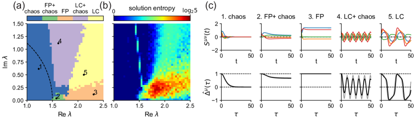
Figure 7: Portrait illustrating the dependence on the leading eigenvalue of $\hat{T}^{\mu\nu,\rho\sigma}$ of the qualitatively distinct dynamic behaviors realized in multiregion networks with asymmetric effective interactions among regions. Here, $R=2$. (a) Portrait of the behavior as a function of the leading eigenvalue. (b) Entropy of the five-way categorical distribution over dynamic behaviors at each point $\lambda$ in (a). (c) Incoming and outgoing currents (top) and two-point functions (bottom) for both regions displaying the dynamic behaviors indicated in (a).

We summarize the results of this analysis in a two-dimensional portrait, Fig. 7(a), showing the most common dynamic behavior across samples of $T^{\mu\nu\rho}$ for each $\lambda$. As the real part of $\lambda$ increases while the imaginary part remains small, the system exhibits a progression of most-common states from chaos with no currents (Fig. 7(c), “chaos”); to a state where the currents settle to a fixed point amid chaotic fluctuations of the units (Fig. 7(c), “FP + chaos”); and, for sufficiently large real part, to a state where a fixed point in the currents suppresses chaos (Fig. 7(c), “FP”). Strikingly, a parallel series of transitions occurs when the imaginary part is larger. In this case, the system transitions from chaos with no currents, as before, to a state where the currents show a limit cycle amid chaotic fluctuations of the units (Fig. 7(c), “LC + chaos”); and, finally, to a state where a limit cycle in the currents suppresses chaos (Fig. 7(c), “LC”). The case where a limit cycle in the currents coexists with chaotic fluctuations is particularly interesting, as it shows that reliable, time-dependent routing through the system can be hidden beneath noisy-looking high-dimensional fluctuations.

How useful is the leading eigenvalue of $\hat{T}^{\mu\nu,\rho\sigma}$ as a predictor of the dynamics? We quantified this by computing the entropy of the empirical distribution over the five possible dynamic states at each $\lambda$, visualized as a heatmap in Fig. 7(b). For large imaginary part of $\lambda$, as the real part is increased from zero, there is a reliable transition from chaos to a limit cycle in the currents coexisting with chaotic fluctuations of the units, with the critical real value near $\text{Re}\lambda=1.5$, the disorder variance parameter. In regions of $\lambda$ space where pure fixed points or pure limit cycles are most common, the behavior is more variable, particularly in parts of this space where different most-common states closely intermingle.

In Fig. 7(a), a dashed circle indicates the support of the bulk of the spectrum of $J^{\mu\nu}_{ij}$. For nontrivial current dynamics to occur, the leading eigenvalue must lie outside this circle; otherwise, these activity modes are swallowed by the bulk. Thus, as the disorder variance parameter increases and the circle expands, a larger-magnitude leading eigenvalue becomes necessary to obtain nontrivial current dynamics. This implies that chaotic fluctuations within regions hinder structured cross-region communication, in analogy with the non-routing mode discussed in Sec. V.3.

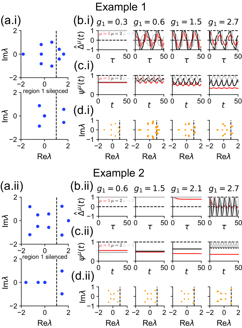
Figure 8: Shaping the multiregion dynamics by modulating disorder and thus signal routing. Examples 1 and 2 show two cases where introducing disorder in region 1 in a network of $R=3$ regions switches the current dynamics from fixed points to limit cycles. (a.i and a.ii) Spectra of $\hat{T}^{\mu\nu,\rho\sigma}$, which have real leading eigenvalues (top), and of the same tensor but with region 1 silenced by setting $T^{\mu 1\rho}=0$ (bottom). Silencing region 1 generates a complex-outlier pair in both cases. (b.i and b.ii) Normalized two-point functions $\hat{\Delta}^{\mu}(\tau)$ from all three regions for increasing levels of disorder in region 1, parameterized by $g^{1}$. (c.i and c.ii) Time-dependent gains $\psi^{\mu}(t)$. (d.i and d.ii) Spectra of $\psi^{\nu}(t)\hat{T}^{\mu\nu,\rho\sigma}$, with different spectra superposed across $t$.

Recall that, in the case of fixed points, switching regions between routing and non-routing modes can tune the geometry and topology of the current-space attractor manifold. We now explore the analogy of this effect in the case of asymmetric effective interactions, where dynamic attractors are possible. We study two examples of networks of $R=3$ regions where increasing the disorder variance parameter $g^{1}$ in region 1, with no disorder in the other regions, induces transitions between fixed-point and limit-cycle attractors in the currents (Fig. 8). To achieve this, in both examples, we construct the effective-interaction tensor such that $\hat{T}^{\mu\nu,\rho\sigma}$ has a real leading eigenvalue, indicative of fixed points, but when entries in $T^{\mu\nu\rho}$ corresponding to region 1 are set to zero, the leading eigenvalues become a complex-conjugate pair, as shown in Figs. 8(a.i) and (a.ii).

We increase $g^{1}$ from zero while keeping $g^{2}=g^{3}=0$ fixed and numerically solve the nonstationary DMFT equations for each value of $g^{1}$. In the first example, for small $g^{1}$, the network sits at a fixed point (Fig. 8(b.i), ${g^{1}=0.3}$). $g^{1}$ surpassing a transition value less than unity gives way to a limit-cycle attractor in the currents (Fig. 8(b.i), ${g^{1}=0.6}$). This limit cycle initially dominates chaotic fluctuations as $g^{1}$ crosses unity (Fig. 8(b.i), ${g^{1}=1.5}$). Further increasing increasing $g^{1}$ induces chaotic fluctuations of the units of region 1, and the low-dimensional communication structure prevents propagation of these high-dimensional fluctuations to other areas (Fig. 8(b.i), ${g^{1}=2.7}$). The second example initially exhibits a fixed-point attractor in the currents (Fig. 8(b.ii), ${g^{1}=0.6}$), even for ${g^{1}>1}$ due to suppression of chaos in region 1 (Fig. 8(b.ii), ${g^{1}=1.5}$). Further increasing $g^{1}$ induces chaotic fluctuations in the units of region 1 alongside a fixed point in the currents (Fig. 8(b.ii), ${g^{1}=2.1}$). For sufficiently large $g^{1}$, the system transitions to a limit cycle in the currents coexisting with chaotic fluctuations localized to the units of region 1 (Fig. 8(b.ii), ${g^{1}=2.7}$). Unlike the first example, no value of $g^{1}$ supports a pure limit cycle in the currents without chaotic fluctuations of the units.

What is the nature of the routing mechanism underlying these disorder-induced phase transitions? This mechanism does not solely involve decreasing the gain $\psi^{1}(t)$ in region 1 to remove it from the network dynamics (despite that our method of identifying appropriate effective-interaction tensors involved excluding region 1). Instead, as $g^{1}$ increases, the gains of all regions stay of order unity (Figs. 8(c.i) and (c.ii)). Increasing disorder can even increase the gain in region 1 (Fig. 8(c.i), ${g=0.3}$ vs. ${g=0.6}$). This indicates that the transitions from fixed-point to limit-cycle attractors in the currents are driven by shaping the alignment of neural activity with particular subspaces rather than traditional gain modulation. Further insight into the nature of time-dependent signal routing through the system can be obtained by studying the spectrum of $\psi^{\nu}(t)\hat{T}^{\mu\nu,\rho\sigma}$ across $t$, which controls the instantaneous linear dynamics of the currents (Figs. 8(d.i) and (d.ii)). The leading eigenvalues hover around unity as the limit cycle unfolds, indicating that the dynamics of the currents are regulated through the sequential activation of subspaces and gain adjustments.

When we allow for fully unconstrained effective interactions, even for the modest values of $R$ considered so far, the dynamics become rich and highly dependent on the specific form of the effective-interaction tensor. This raises the question of whether we can glean general insights when the number of regions is large, as is the case in real neural circuits. To investigate this, we examine a model of $R=5$ regions and asymmetric effective interactions. We randomly sample an effective-interaction tensor that yields complex-conjugate leading eigenvalues, along with several other real and complex unstable modes (Fig. 9(a)). Without disorder, this effective-interaction tensor produces an intricate limit cycle in the currents (Fig. 9(b), $g=0$). Increasing the disorder variance parameter $g$ uniformly across regions reduces the complexity of the limit cycle due to chaotic fluctuations disrupting communication between regions (Fig. 9(b), $g=1$ and $g=2$). For sufficiently large $g$, the currents vanish as disordered connectivity within regions overtakes structured communication (Fig. 9(b), $g=3$). The gradual transition from a complex to a simple limit cycle, and eventually to its absence with increasing disorder, can be understood in terms of the growing radius of the spectral bulk, which swallows more and more outlier modes linked to the dynamics of the currents (Fig. 9(a), circles). Inspection of the gains $\psi^{\mu}(t)$ reveals that, rather than vanishing, gains remain of order unity (Fig. 9(c)). However, gains exhibit less complexity across time for larger $g$. Moreover, the leading eigenvalues of the spectrum of $\psi^{\nu}(t)\hat{T}^{\mu\nu,\rho\sigma}$ hover around unity, with a diminishing number of modes crossing the stability line as $g$ increases (Fig. 9(d)).

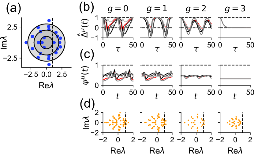
Figure 9: Relationship between disorder and current-variable dynamic complexity in a network of $R=5$ regions. (a) Spectrum of $\hat{T}^{\mu\nu,\rho\sigma}$. Shaded circles represent the support of the bulk of the spectrum of $J^{\mu\nu}_{ij}$ for disorder levels $g\in\{0,1,2,3\}$. (b–d) Same information is Figs. 8(b–d), namely, (b) normalized two-point functions, (c) time-dependent gains, and (d) gain-modulated effective-interaction spectra.

VII Discussion

In the cases of both fixed-point and dynamic attractors, we have shown that adjusting the effective interactions or levels of disorder can shift how signals are routed through the network by activating different subspaces. This shifting does not simply silence regions, i.e., it does not reduce the gain of a region to zero. Instead, it alters which subspaces are active, causing phase transitions where currents become zero or nonzero while the gains remain of order unity. We note that to achieve phase transitions to exactly zero currents, reciprocal effective interactions among regions are required. For instance, in a feedforward chain $1\rightarrow 2\rightarrow 3$, where region 1 sends signals to region 3 via region 2, introducing any level of disorder or low-rank connectivity in region 2 does not entirely stop communication, but does attenuate it through reducing the gain in region 2, due to the feedforward communication structure.

Neural projections between brain regions are characterized by diverse biological constraints, such as excitatory-only connections, sparsity, and layer-specificity. In our approach, we assume these projections have a low-rank structure. This assumption is inspired by experimental findings of communication subspaces and abstracts away these specific biological details to facilitate general insights.

In particular, we focused on rank-one communication subspaces with jointly Gaussian loadings. This connectivity provides a starting point for studying more complicated forms of communication between areas. For example, we can extend our rank-one connectivity model to rank-$K$ subspaces, facilitating richer, higher-dimensional communication. Crucially, maintaining the ranks of these subspaces as intensive prevents high-dimensional chaotic fluctuations from propagating between regions, preserving the modularity of the disorder-based gating mechanism. While increasing the rank increases the number dynamic variables in the mean-field picture (namely, by a factor of $K$), the Gaussian distribution over loadings restricts the complexity of their effective interactions in the DMFT. An alternative is to use a mixture-of-Gaussians distribution with $C$ components, allowing for more complex interactions [55, 56]. Together, these extensions expand the effective-interaction tensor by three indices, detailed in a tensor diagram in Fig. 10. Finally, one could arrange regions on a spatial lattice, as was done by Hansel and Sompolinsky [57].

An additional extension to consider is the inclusion of disorder in the cross-region couplings. The connectivity in this scenario is represented as

$$J^{\mu\nu}_{ij}=\chi^{\mu\nu}_{ij}+m^{\mu\nu}_{i}n^{\mu\nu}_{j},$$ (37)

where $\left\langle(\chi_{ij}^{\mu\nu})^{2}\right\rangle_{\bm{J}}=G^{\mu\nu}/N$. This combines the model of Aljadeff et al. [34] with our communication-subspace model. In this modified system, the current dynamics are unchanged, but two-point function dynamics, Eq. 13, and thus the time-dependent gains, are updated to

$$(1+\partial_{t})(1+\partial_{t^{\prime}})\Delta^{\mu}(t,t^{\prime})=\sum_{\nu}G^{\mu\nu}C^{\mu}(t,t^{\prime})\\ +\sum_{\nu,\rho}U^{\mu\nu\rho}H^{\mu\nu}(t)H^{\mu\rho}(t^{\prime}).$$ (38)

The primary new effect is the propagation of chaotic fluctuations between regions due to the high-dimensional cross-region connectivity, captured by the coupling of $\Delta^{\mu}(t,t^{\prime})$ to other $C^{\nu}(t,t^{\prime})$ for $\nu\neq\mu$ in Eq. 38. Thus, the modularity of the disorder-based gating mechanism may not be preserved. Nevertheless, this propagation of chaotic fluctuations could shape the current dynamics in interesting ways.

We now situate our model within a line of existing research. Setting aside disorder, our model involves a blockwise low-rank coupling matrix, an embodiment of a broader idea where neurons are assigned group identities and coupling statistics are based on these identities. Another embodiment of this idea is the low-rank mixture-of-Gaussians model proposed by [55, 56], where the coupling matrix is a sum of rank-one outer products with mixture-of-Gaussians loadings. In this framework, each neuronal group corresponds to a Gaussian mixture component. Our multiregion network model, of $R$ regions, is a special case of a low-rank mixture-of-Gaussians network with rank $R^{2}$ and $R$ mixture components (Appendix A). Furthermore, as described above, multiregion networks can themselves be generalized to have rank-$K$ communication subspaces and $C$ Gaussian-mixture components. This extension can be captured by a low-rank mixture-of-Gaussians construction with $KR^{2}$ rank-one terms and $CR$ mixture components. Compared to generic networks in the low-rank mixture-of-Gaussians class, multiregion networks possess a far greater degree of structure. An interesting question is whether the inductive bias corresponding to multiregion networks is advantageous in constructing models within this class.

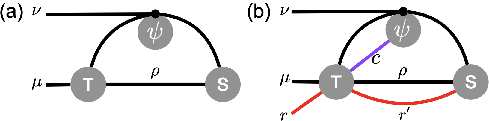
Figure 10: Tensor diagrams illustrating the extension of multiregion networks to higher-rank communication subspaces with mixture-of-Gaussians loadings. (a) Form of $(1+\partial_{t})S^{\mu\nu}(t)$ in the multiregion network we have studied. (b) Form of $(1+\partial_{t})S^{\mu\nu}_{r}(t)$ in the aforementioned extension (in this case, the currents acquire an additional $r$ index that runs over rank-one components). The diagram has two new internal lines corresponding to contractions over mixture components ($c$) and rank-one components ($r^{\prime}$).

In our model, modifying the state of the network, for example, by changing whether a region is in routing or non-routing mode, requires altering synaptic couplings. This could occur dynamically through neuromodulation. An interesting alternative is to use external inputs to control routing. For instance, consider a region that cannot transmit signals due to disorder-induced chaotic fluctuations of the units. If an external stimulus suppresses these fluctuations, the region could gain the ability to transmit signals. This behavior aligns with the experimental observation that neuronal variability quenches at stimulus onset, and suggests that this reduction facilitates cross-region communication [27]. To model this, we can integrate additional input vectors into our framework. This would expand the mean-field equations to include new effective interactions encoding the overlap between the vectors defining the recurrent connectivity and the input vectors. A similar approach was explored by Barbosa et al. [22], who studied a two-region network with a specific configuration of the effective interactions.

A notable aspect of our model and theoretical approach is its alignment with existing methods for neural-data analysis. Specifically, the technique developed by [9] for analyzing multiregion neural recordings involves training a recurrent network to mimic the data, then decomposing the activity in terms of cross-region currents. Intriguingly, our model’s low-dimensional mean-field dynamics offer a closed description in these currents, rather than relying solely on single-region quantities such as two-point functions. This alignment strongly supports the use of current-based analyses in neural data interpretation. Furthermore, our model could be adapted to fit multiregion neural data using approaches akin to those in Valente et al. [58]. Subsequently reducing the model to the mean-field description we derived could provide insights into the dynamics of the fitted model. This positions our work as a bridge connecting practical recurrent-network-based data analysis methods to a deeper analytical understanding of network dynamics.

Another data-driven application of our framework lies in analyzing large-scale connectome data [59]. For example, large-scale reconstructions of neurons and their connections are now available for flies [60, 61], parts of the mammalian cortex [62], and in some other organisms [63]. For connectome datasets where regions are identified, the cross-region connectivity could be approximated as having a low-rank structure, allowing for a reduction using our mean-field framework. This enables a comparison of predicted neuronal dynamics with recorded activity. In scenarios where regions are not already defined, our framework suggests solving the “inverse problem,” namely, determining a partitioning of neurons into regions such that the cross-region connectivity is well approximated by low-rank matrices. Developing a special clustering algorithm for this purpose and applying it to connectome data, such as from the fly, would be interesting. Even in cases where anatomical knowledge suggests certain region definitions, identifying “unsupervised regions” based on the assumption of low-rank cross-region interactions could offer an interesting new functional perspective on regional delineation.

VIII Acknowledgements

We are extremely grateful to L.F. Abbott for his advice on this work. We thank Albert J. Wakhloo for comments on the manuscript, as well as Rainer Engelken, Haim Sompolinsky, Ashok Litwin-Kumar, and members of the Litwin-Kumar group for helpful discussions. D.G.C. was supported by the Kavli Foundation Endowment and Gatsby Charitable Foundation award GAT3708. M.B. was supported by NIH award R01EB029858.

Appendix A Locating multiregion networks in the space of low-rank mixture-of-Gaussians networks

Here, we demonstrate via an explicit construction that multiregion networks are a special case of the low-rank mixture-of-Gaussians model, a framework extensively studied in the literature [55, 56, 58, 64, 65, 66]. We demonstrate this mapping in the disorder-free case. Consider a low-rank network where the rank-one terms are indexed by $r$ (or $r^{\prime}$), neurons are indexed by $i$ (or $j$), and the coupling matrix $W_{ij}$ is defined as

$$W_{ij}=\sum_{r}v^{r}_{i}w^{r}_{j}.$$ (39)

The components of the vectors $v^{r}_{i}$ and $w^{r}_{i}$ follow a mixture-of-Gaussians distribution with i.i.d. sampling across the neuron index, $i$. Each mixture component has zero mean. The second-order statistics are given by

$$\left\langle w^{r}_{i}v^{r^{\prime}}_{i}\right\rangle_{c} =[\text{num. components}]\times t^{rr^{\prime}}[c],$$ (40)

$$\left\langle v^{r}_{i}v^{r^{\prime}}_{i}\right\rangle_{c} =[\text{num. components}]\times u^{rr^{\prime}}[c],$$ (41)

where $\left\langle\cdot\right\rangle_{c}$ denotes an average in mixture component $c$. We assume that all mixture components have equal probability. With these definitions, the mean-field equations were shown to be

$$(1+\partial_{t})\kappa^{r}(t) =\sum_{r^{\prime}}\left[\sum_{c}\psi^{c}(t)t^{rr^{\prime}}[c]\right]\kappa^{r^{\prime}}(t),$$ (42)

$$\psi^{c}(t) =\psi\left(\sum_{r,r^{\prime}}u^{rr^{\prime}}[c]\kappa^{r}(t)\kappa^{r^{\prime}}(t)\right),$$ (43)

where $\psi(\Delta)$ is given for the error-function nonlinearity by Eq. 15b.

Toward making a multiregion network emerge from these equations, we consider $R^{2}$ rank-one terms and $R$ mixture components, and substitute $r\rightarrow(\mu,\nu)$, $r^{\prime}\rightarrow(\rho,\sigma)$, and $c\rightarrow\alpha$. The second-order statistics are constructed as follows:

$$t^{\mu\nu,\rho\sigma}[\alpha] =\delta^{\alpha\nu}\delta^{\alpha\rho}T^{\mu\nu\sigma},$$ (44)

$$u^{\mu\nu,\rho\sigma}[\alpha] =\delta^{\alpha\mu}\delta^{\alpha\rho}U^{\alpha\nu\sigma},$$ (45)

where $T^{\mu\nu\rho}$ and $U^{\mu\nu\rho}$ are the tensors defining the multiregion network of interest. Under this construction, the mean-field equations transform into those for multiregion networks.

We have reproduced the mean-field equations of the multiregion network, but do realizations of the couplings $W_{ij}$ exhibit the blockwise low-rank structure of multiregion networks? Consider the rank-one term $v^{\mu\nu}_{i}w^{\mu\nu}_{j}$ in this construction. Note that $\left\langle(v^{\mu\nu}_{i})^{2}\right\rangle_{\alpha}$ is proportional to $\delta^{\alpha\mu}$. Thus, only the rows corresponding to mixture component $\mu$ are nonzero in this rank-one term. Now, the second-order statistics among the “$w$” vectors are not relevant to the mean-field equations. But, if we assume that $\left\langle(w^{\mu\nu}_{i}))^{2}\right\rangle_{\alpha}$ is proportional to $\delta^{\alpha\nu}$, only the columns corresponding to mixture component $\nu$ are nonzero in this rank-one term. Thus, in rank-one term $(\mu,\nu)$, the nonzero entries form a submatrix corresponding to rows in mixture component $\mu$ and columns in mixture component $\nu$. Given that there is a single rank-one term for each $(\mu,\nu)$, a rank-one submatrix is present at every $(\mu,\nu)$ block of $W_{ij}$.

In summary, we have located multiregion networks in the space of low-rank mixture-of-Gaussians networks. In particular, when the $u^{rr^{\prime}}[c]$ and $U^{\mu\nu\rho}$ terms are fixed, multiregion networks lie on an $R^{3}$-dimensional manifold in the $R^{5}$-dimensional space of rank-$R^{2}$ networks with $R$ mixture components. In this sense, multiregion networks possess a high degree of structure compared to generic networks in the low-rank mixture-of-Gaussians class.

References

- Felleman and Van Essen [1991] D. J. Felleman and D. C. Van Essen, Distributed hierarchical processing in the primate cerebral cortex., Cerebral Cortex 1, 1 (1991).
- Ito et al. [2014] K. Ito, K. Shinomiya, M. Ito, J. D. Armstrong, G. Boyan, V. Hartenstein, S. Harzsch, M. Heisenberg, U. Homberg, A. Jenett, H. Keshishian, L. L. Restifo, W. Rössler, J. H. Simpson, N. J. Strausfeld, R. Strauss, and L. B. Vosshall, A systematic nomenclature for the insect brain, Neuron 81, 755 (2014).
- Randlett et al. [2015] O. Randlett, C. L. Wee, E. A. Naumann, O. Nnaemeka, D. Schoppik, J. E. Fitzgerald, R. Portugues, A. M. Lacoste, C. Riegler, F. Engert, and A. F. Schier, Whole-brain activity mapping onto a zebrafish brain atlas, Nature Methods 2015 12:11 12, 1039 (2015).
- Wang et al. [2020] Q. Wang, S.-L. Ding, Y. Li, J. Royall, D. Feng, P. Lesnar, N. Graddis, M. Naeemi, B. Facer, A. Ho, et al., The allen mouse brain common coordinate framework: a 3d reference atlas, Cell 181, 936 (2020).
- Markov et al. [2011] N. T. Markov, P. Misery, A. Falchier, C. Lamy, J. Vezoli, R. Quilodran, M. Gariel, P. Giroud, M. Ercsey-Ravasz, L. Pilaz, et al., Weight consistency specifies regularities of macaque cortical networks, Cerebral Cortex 21, 1254 (2011).
- Ecker et al. [2014] A. S. Ecker, P. Berens, R. J. Cotton, M. Subramaniyan, G. H. Denfield, C. R. Cadwell, S. M. Smirnakis, M. Bethge, and A. S. Tolias, State dependence of noise correlations in macaque primary visual cortex, Neuron 82, 235 (2014).
- Lin et al. [2015] I. C. Lin, M. Okun, M. Carandini, and K. D. Harris, The nature of shared cortical variability, Neuron 87, 644 (2015).
- Andalman et al. [2019] A. S. Andalman, V. M. Burns, M. Lovett-Barron, M. Broxton, B. Poole, S. J. Yang, L. Grosenick, T. N. Lerner, R. Chen, T. Benster, P. Mourrain, M. Levoy, K. Rajan, and K. Deisseroth, Neuronal dynamics regulating brain and behavioral state transitions, Cell 177, 970 (2019).
- Perich et al. [2020a] M. G. Perich, C. Arlt, S. Soares, M. E. Young, C. P. Mosher, J. Minxha, E. Carter, U. Rutishauser, P. H. Rudebeck, C. D. Harvey, et al., Inferring brain-wide interactions using data-constrained recurrent neural network models, BioRxiv , 2020 (2020a).
- Okazawa and Kiani [2023] G. Okazawa and R. Kiani, Neural mechanisms that make perceptual decisions flexible (2023).
- Fang and Stachenfeld [2023] C. Fang and K. L. Stachenfeld, Predictive auxiliary objectives in deep RL mimic learning in the brain, arXiv preprint arXiv:2310.06089 (2023).
- Jun et al. [2017] J. J. Jun, N. A. Steinmetz, J. H. Siegle, D. J. Denman, M. Bauza, B. Barbarits, A. K. Lee, C. A. Anastassiou, A. Andrei, Ç. Aydin, M. Barbic, T. J. Blanche, V. Bonin, J. Couto, B. Dutta, S. L. Gratiy, D. A. Gutnisky, M. Häusser, B. Karsh, P. Ledochowitsch, C. M. Lopez, C. Mitelut, S. Musa, M. Okun, M. Pachitariu, J. Putzeys, P. D. Rich, C. Rossant, W. L. Sun, K. Svoboda, M. Carandini, K. D. Harris, C. Koch, J. O’Keefe, and T. D. Harris, Fully integrated silicon probes for high-density recording of neural activity, Nature 551, 232 (2017).
- Machado et al. [2022] T. A. Machado, I. V. Kauvar, and K. Deisseroth, Multiregion neuronal activity: the forest and the trees (2022).
- Manley et al. [2024] J. Manley, J. Demas, H. Kim, F. Martinez Traub, and A. Vaziri, Simultaneous, cortex-wide and cellular-resolution neuronal population dynamics reveal an unbounded scaling of dimensionality with neuron number, bioRxiv , 2024 (2024).
- Musall et al. [2019] S. Musall, M. T. Kaufman, A. L. Juavinett, S. Gluf, and A. K. Churchland, Single-trial neural dynamics are dominated by richly varied movements, Nature neuroscience 22, 1677 (2019).
- Steinmetz et al. [2019] N. A. Steinmetz, P. Zatka-Haas, M. Carandini, and K. D. Harris, Distributed coding of choice, action and engagement across the mouse brain, Nature 576, 266 (2019).
- Brain Laboratory et al. [2023] I. Brain Laboratory, B. Benson, J. Benson, D. Birman, N. Bonacchi, M. Carandini, J. A. Catarino, G. A. Chapuis, A. K. Churchland, Y. Dan, P. Dayan, E. E. DeWitt, T. A. Engel, M. Fabbri, M. Faulkner, I. Rani Fiete, C. Findling, L. Freitas-Silva, B. Gerçek, K. D. Harris, M. Häusser, S. B. Hofer, F. Hu, F. Hubert, J. M. Huntenburg, A. Khanal, C. Krasniak, C. Langdon, P. Y. P Lau, Z. F. Mainen, G. T. Meijer, N. J. Miska, T. D. Mrsic-Flogel, J.-P. Noel, K. Nylund, A. Pan-Vazquez, A. Pouget, C. Rossant, N. Roth, R. Schaeffer, M. Schartner, Y. Shi, K. Z. Socha, N. A. Steinmetz, K. Svoboda, A. E. Urai, M. J. Wells, S. Jon West, M. R. Whiteway, O. Winter, and I. B. Witten, A brain-wide map of neural activity during complex behaviour, bioRxiv , 2023.07.04.547681 (2023).
- Schaffer et al. [2023] E. S. Schaffer, N. Mishra, M. R. Whiteway, W. Li, M. B. Vancura, J. Freedman, K. B. Patel, V. Voleti, L. Paninski, E. M. Hillman, et al., The spatial and temporal structure of neural activity across the fly brain, Nature Communications 14, 5572 (2023).
- Pinto et al. [2019] L. Pinto, K. Rajan, B. DePasquale, S. Y. Thiberge, D. W. Tank, and C. D. Brody, Task-dependent changes in the large-scale dynamics and necessity of cortical regions, Neuron 104, 810 (2019).
- Michaels et al. [2020] J. A. Michaels, S. Schaffelhofer, A. Agudelo-Toro, and H. Scherberger, A goal-driven modular neural network predicts parietofrontal neural dynamics during grasping, Proceedings of the national academy of sciences 117, 32124 (2020).
- Chen et al. [2021] G. Chen, B. Kang, J. Lindsey, S. Druckmann, and N. Li, Modularity and robustness of frontal cortical networks, Cell 184, 3717 (2021).
- Barbosa et al. [2023] J. Barbosa, R. Proville, C. C. Rodgers, M. R. DeWeese, S. Ostojic, and Y. Boubenec, Early selection of task-relevant features through population gating, Nature Communications 14, 6837 (2023).
- Nair et al. [2023] A. Nair, T. Karigo, B. Yang, S. Ganguli, M. J. Schnitzer, S. W. Linderman, D. J. Anderson, and A. Kennedy, An approximate line attractor in the hypothalamus encodes an aggressive state, Cell 186, 178 (2023).
- Perich and Rajan [2020] M. G. Perich and K. Rajan, Rethinking brain-wide interactions through multi-region ‘network of networks’ models, Current opinion in neurobiology 65, 146 (2020).
- Mastrogiuseppe and Ostojic [2018] F. Mastrogiuseppe and S. Ostojic, Linking connectivity, dynamics, and computations in low-rank recurrent neural networks, Neuron 99, 609 (2018).
- Pereira-Obilinovic et al. [2023] U. Pereira-Obilinovic, J. Aljadeff, and N. Brunel, Forgetting leads to chaos in attractor networks, Physical Review X 13, 10.1103/PhysRevX.13.011009 (2023), arXiv:2112.00119 .
- Churchland et al. [2010] M. M. Churchland, B. M. Yu, J. P. Cunningham, L. P. Sugrue, M. R. Cohen, G. S. Corrado, W. T. Newsome, A. M. Clark, P. Hosseini, B. B. Scott, et al., Stimulus onset quenches neural variability: a widespread cortical phenomenon, Nature neuroscience 13, 369 (2010).
- Rajan et al. [2010] K. Rajan, L. Abbott, and H. Sompolinsky, Stimulus-dependent suppression of chaos in recurrent neural networks, Physical review e 82, 011903 (2010).
- Gallego et al. [2017] J. A. Gallego, M. G. Perich, L. E. Miller, and S. A. Solla, Neural manifolds for the control of movement, Neuron 94, 978 (2017).
- Abbott [2006] L. Abbott, Where are the switches on this thing, 23 Problems in systems neuroscience , 423 (2006).
- Cichocki [2014] A. Cichocki, Tensor networks for big data analytics and large-scale optimization problems, arXiv preprint arXiv:1407.3124 (2014).
- Bridgeman and Chubb [2017] J. C. Bridgeman and C. T. Chubb, Hand-waving and interpretive dance: an introductory course on tensor networks, Journal of Physics A 50, 223001 (2017).
- Sompolinsky et al. [1988] H. Sompolinsky, A. Crisanti, and H.-J. Sommers, Chaos in random neural networks, Physical review letters 61, 259 (1988).
- Aljadeff et al. [2015] J. Aljadeff, M. Stern, and T. Sharpee, Transition to chaos in random networks with cell-type-specific connectivity, Physical review letters 114, 088101 (2015).
- Semedo et al. [2019] J. D. Semedo, A. Zandvakili, C. K. Machens, M. Y. Byron, and A. Kohn, Cortical areas interact through a communication subspace, Neuron 102, 249 (2019).
- Semedo et al. [2022] J. D. Semedo, A. I. Jasper, A. Zandvakili, A. Krishna, A. Aschner, C. K. Machens, A. Kohn, and B. M. Yu, Feedforward and feedback interactions between visual cortical areas use different population activity patterns, Nature communications 13, 1099 (2022).
- Perich et al. [2020b] M. G. Perich, S. Conti, M. Badi, A. Bogaard, B. Barra, S. Wurth, J. Bloch, G. Courtine, S. Micera, M. Capogrosso, et al., Motor cortical dynamics are shaped by multiple distinct subspaces during naturalistic behavior, BioRxiv , 2020 (2020b).
- Kondapavulur et al. [2022] S. Kondapavulur, S. M. Lemke, D. Darevsky, L. Guo, P. Khanna, and K. Ganguly, Transition from predictable to variable motor cortex and striatal ensemble patterning during behavioral exploration, Nature Communications 13, 2450 (2022).
- Srinath et al. [2021] R. Srinath, D. A. Ruff, and M. R. Cohen, Attention improves information flow between neuronal populations without changing the communication subspace, Current Biology 31, 5299 (2021).
- MacDowell et al. [2023] C. J. MacDowell, A. Libby, C. I. Jahn, S. Tafazoli, and T. J. Buschman, Multiplexed subspaces route neural activity across brain-wide networks, bioRxiv , 2023 (2023).
- Note [1] Specifying the covariances , , and for is unnecessary for both the mean-field description and for sampling couplings. This is because such covariances, when interpreted as vector contractions, are not physically valid; the relevant vectors only have the same number of components in our model for simplicity, but in general their numbers of components could differ across regions by intensive ratios.
- Engelken and Goedeke [2022] R. Engelken and S. Goedeke, A time-resolved theory of information encoding in recurrent neural networks, Advances in Neural Information Processing Systems 35, 35490 (2022).
- Turing [1990] A. M. Turing, The chemical basis of morphogenesis, Bulletin of mathematical biology 52, 153 (1990).
- Sorscher et al. [2019] B. Sorscher, G. Mel, S. Ganguli, and S. Ocko, A unified theory for the origin of grid cells through the lens of pattern formation, Advances in neural information processing systems 32 (2019).
- Cunningham and Yu [2014] J. P. Cunningham and B. M. Yu, Dimensionality reduction for large-scale neural recordings, Nature neuroscience 17, 1500 (2014).
- Hopfield [1982] J. J. Hopfield, Neural networks and physical systems with emergent collective computational abilities., Proceedings of the national academy of sciences 79, 2554 (1982).
- Ben-Yishai et al. [1995] R. Ben-Yishai, R. L. Bar-Or, and H. Sompolinsky, Theory of orientation tuning in visual cortex., Proceedings of the National Academy of Sciences 92, 3844 (1995).
- Kim et al. [2017] S. S. Kim, H. Rouault, S. Druckmann, and V. Jayaraman, Ring attractor dynamics in the drosophila central brain, Science 356, 849 (2017).
- Chaudhuri et al. [2019] R. Chaudhuri, B. Gerçek, B. Pandey, A. Peyrache, and I. Fiete, The intrinsic attractor manifold and population dynamics of a canonical cognitive circuit across waking and sleep, Nature neuroscience 22, 1512 (2019).
- Burak and Fiete [2009] Y. Burak and I. R. Fiete, Accurate path integration in continuous attractor network models of grid cells, PLoS Computational Biology 5, e1000291 (2009).
- Gardner et al. [2022] R. J. Gardner, E. Hermansen, M. Pachitariu, Y. Burak, N. A. Baas, B. A. Dunn, M.-B. Moser, and E. I. Moser, Toroidal topology of population activity in grid cells, Nature 602, 123 (2022).
- Motzkin et al. [1953] T. S. Motzkin, H. Raiffa, G. L. Thompson, and R. M. Thrall, The double description method, Contributions to the Theory of Games 2, 51 (1953).
- Fukuda [1997] K. Fukuda, cdd/cdd+ reference manual, Institute for Operations Research, ETH-Zentrum , 91 (1997).
- Van der Maaten and Hinton [2008] L. Van der Maaten and G. Hinton, Visualizing data using t-sne., Journal of machine learning research 9 (2008).
- Beiran et al. [2021] M. Beiran, A. Dubreuil, A. Valente, F. Mastrogiuseppe, and S. Ostojic, Shaping dynamics with multiple populations in low-rank recurrent networks, Neural Computation 33, 1572 (2021).
- Dubreuil et al. [2022] A. Dubreuil, A. Valente, M. Beiran, F. Mastrogiuseppe, and S. Ostojic, The role of population structure in computations through neural dynamics, Nature neuroscience 25, 783 (2022).
- Hansel and Sompolinsky [1993] D. Hansel and H. Sompolinsky, Solvable model of spatiotemporal chaos, Physical review letters 71, 2710 (1993).
- Valente et al. [2022] A. Valente, J. W. Pillow, and S. Ostojic, Extracting computational mechanisms from neural data using low-rank rnns, Advances in Neural Information Processing Systems 35, 24072 (2022).
- Abbott et al. [2020] L. F. Abbott, D. D. Bock, E. M. Callaway, W. Denk, C. Dulac, A. L. Fairhall, I. Fiete, K. M. Harris, M. Helmstaedter, V. Jain, et al., The mind of a mouse, Cell 182, 1372 (2020).
- Zheng et al. [2018] Z. Zheng, J. S. Lauritzen, E. Perlman, C. G. Robinson, M. Nichols, D. Milkie, O. Torrens, J. Price, C. B. Fisher, N. Sharifi, et al., A complete electron microscopy volume of the brain of adult drosophila melanogaster, Cell 174, 730 (2018).
- Scheffer et al. [2020] L. K. Scheffer, C. S. Xu, M. Januszewski, Z. Lu, S.-y. Takemura, K. J. Hayworth, G. B. Huang, K. Shinomiya, J. Maitlin-Shepard, S. Berg, et al., A connectome and analysis of the adult drosophila central brain, Elife 9, e57443 (2020).
- Winnubst et al. [2019] J. Winnubst, E. Bas, T. A. Ferreira, Z. Wu, M. N. Economo, P. Edson, B. J. Arthur, C. Bruns, K. Rokicki, D. Schauder, et al., Reconstruction of 1,000 projection neurons reveals new cell types and organization of long-range connectivity in the mouse brain, Cell 179, 268 (2019).
- Hildebrand et al. [2017] D. G. C. Hildebrand, M. Cicconet, R. M. Torres, W. Choi, T. M. Quan, J. Moon, A. W. Wetzel, A. Scott Champion, B. J. Graham, O. Randlett, et al., Whole-brain serial-section electron microscopy in larval zebrafish, Nature 545, 345 (2017).
- Beiran et al. [2023] M. Beiran, N. Meirhaeghe, H. Sohn, M. Jazayeri, and S. Ostojic, Parametric control of flexible timing through low-dimensional neural manifolds, Neuron 111, 739 (2023).
- Cimeša et al. [2023] L. Cimeša, L. Ciric, and S. Ostojic, Geometry of population activity in spiking networks with low-rank structure, PLoS Computational Biology 19, e1011315 (2023).
- Shao and Ostojic [2023] Y. Shao and S. Ostojic, Relating local connectivity and global dynamics in recurrent excitatory-inhibitory networks, PLOS Computational Biology 19, e1010855 (2023).