Adversarial Feature Alignment: Balancing Robustness and Accuracy in Deep Learning via Adversarial Training

Abstract.

Deep learning models continue to advance in accuracy, yet they remain vulnerable to adversarial attacks, which often lead to the misclassification of adversarial examples. Adversarial training is used to mitigate this problem by increasing robustness against these attacks. However, this approach typically reduces a model’s standard accuracy on clean, non-adversarial samples. The necessity for deep learning models to balance both robustness and accuracy for security is obvious, but achieving this balance remains challenging, and the underlying reasons are yet to be clarified.

This paper proposes a novel adversarial training method called Adversarial Feature Alignment (AFA), to address these problems. Our research unveils an intriguing insight: misalignment within the feature space often leads to misclassification, regardless of whether the samples are benign or adversarial. AFA mitigates this risk by employing a novel optimization algorithm based on contrastive learning to alleviate potential feature misalignment. Through our evaluations, we demonstrate the superior performance of AFA. The baseline AFA delivers higher robust accuracy than previous adversarial contrastive learning methods while minimizing the drop in clean accuracy to 1.86% and 8.91% on CIFAR10 and CIFAR100, respectively, in comparison to cross-entropy. We also show that joint optimization of AFA and TRADES, accompanied by data augmentation using a recent diffusion model, achieves state-of-the-art accuracy and robustness.

1. Introduction

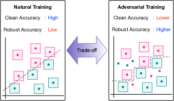
(a) Robustness-Accuracy Tradeoff of DNNs

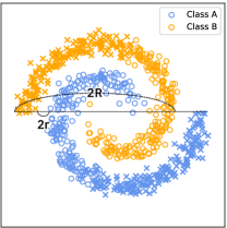
(b) Misaligned distribution (not enough)

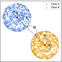
(c) Aligned distribution (helpful)

Figure 1. Visual illustrations of data distribution manifolds with colors indicating sample labels. (a) Illustrates the robustness-accuracy tradeoff problem regarding standard clean accuracy and robust accuracy. (b) Shows misaligned distribution where test sample ’x’ might differ in color from its nearest training sample ’o’, despite large class distances. (c) Depicts aligned distribution satisfying both separation and clustering, ensuring test sample ’x’ matches the color of training sample ’o’ if the minimum class distance is at least twice the radius of ’o’.

Deep Neural Networks (DNNs), despite their high accuracy on clean samples, are notably susceptible to adversarial examples. These examples, involving test inputs with imperceptible perturbations, can lead to misclassifications, posing significant concerns in safety-critical domains such as autonomous driving and medical diagnosis (Szegedy et al., 2013; Papernot et al., 2016; Dong et al., 2018; Moosavi-Dezfooli et al., 2016; Carlini and Wagner, 2017; Kurakin et al., 2016). Adversarial training has emerged as a crucial defensive technique over the past decade, enhancing the security of deep learning systems against such adversarial threats (Goodfellow et al., 2014; Madry et al., 2017; Tramèr et al., 2017; Kurakin et al., 2016). Unlike methods that rely on auxiliary models (Meng and Chen, 2017; Ma et al., 2018), adversarial training directly enhances a classifier’s robustness. It focuses on learning robust parameters to minimize adversarial losses, increasingly being generalized and certified across various samples. Recent advancements have aimed to guarantee or raise the lower bound of DNN robustness against $\epsilon$-bounded adversarial perturbations (Li et al., 2023a; Zhang et al., 2023a; Yuan et al., 2023). Initially focused on image classification, the concept of robust training is now expanding into other areas, including federated learning (Zizzo et al., 2020; Zhang et al., 2023b; Li et al., 2023b; Reisizadeh et al., 2020) and malware detection (Lucas et al., 2023), marking a significant evolution in the field.

The primary goal of adversarial training in DNNs is to enhance robustness against adversarial examples. However, this often comes at the cost of reduced accuracy on clean samples, presenting a significant robustness-accuracy tradeoff (Tsipras et al., 2018; Zhang et al., 2019). This tradeoff is particularly problematic in real-world applications, where the prevalence of normal samples means a robust but less accurate model may underperform compared to a standard model. For instance, in anomaly detection tasks like malware or fraud detection, this could lead to an unacceptable increase in false positives, compromising the model’s practical utility. While the robustness-accuracy tradeoff was once thought unavoidable (Tsipras et al., 2018), recent research has offered new perspectives. Yang et al. (Yang et al., 2020) suggested that certain dataset characteristics, like class separation, might mitigate this tradeoff. However, our work argues that this property alone is insufficient, as shown in Figure 1(b). We propose two new data distribution properties: clustering and alignment. Clustering refers to the proximity of samples within a class, while alignment combines separation and clustering. We demonstrate that misclassification is virtually eliminated in datasets that exhibit these properties. See Figure 1(c).

Our analysis of actual datasets reveals a critical finding: separation does not imply alignment, leading to potential misclassification risks. This suggests that the tradeoff issue is inherent in the input space, contrary to the finding of (Yang et al., 2020). Therefore, we propose that aligning the feature space, particularly at the penultimate layer output of neural networks, is crucial. Our findings indicate that existing training algorithms do not effectively align the feature space, leading to misclassification. This insight underscores the necessity of a training algorithm that aligns the feature space to resolve the tradeoff in neural networks.

We propose Adversarial Feature Alignment (AFA), a novel adversarial training method targeting DNN feature extractors to improve the robustness-accuracy tradeoff. AFA aims to identify and minimize risks from adversarial examples causing feature space misalignment. Utilizing contrastive learning (Chen et al., 2020a; Khosla et al., 2020), known for its efficacy in feature space generalization, AFA operates under three key principles: (1) using adversarial examples that lead to the most significant feature misalignment, (2) ensuring these examples adhere to the class-label data manifold, and (3) providing precise guidance for their alignment. We have developed a new fully-supervised contrastive loss function, the AFA loss, that meets these criteria and is optimized through a min-max approach. Figure 3 illustrates the overview of our approach. AFA uniquely creates adversarial examples that amplify feature distance from their true class while reducing it from other classes, targeting the worst-case scenario for separation and clustering. Unlike previous self-supervised adversarial contrastive learning methods that struggle with class collision problems (Kim et al., 2020; Jiang et al., 2020; Ho and Nvasconcelos, 2020; Fan et al., 2021; Yu et al., 2022), AFA excels in aligning features robustly across classes, significantly enhancing the security and practicality of deep neural network training. We propose two distinct training strategies using AFA loss: initially pre-training the feature extractor with AFA followed by fine-tuning the linear classifier, and alternatively, training the entire network through joint optimization of adversarial and AFA losses. The joint optimization of AFA further improves the state-of-the-art accuracy and robustness when combined with the recent approach (Wang et al., 2023) that leverages a diffusion model (Karras et al., 2022) for data augmentation. Our experimental results confirm that AFA outperforms existing methods in both accuracy and robustness, and its efficacy is further amplified when integrated with recent diffusion model-based data augmentation techniques.

Contributions. This paper makes the following key contributions:

• We offer a new approach to address the robustness-accuracy tradeoff, focusing on aligning the separated data distribution through clustering within each class. Contrary to previous beliefs, our experiments reveal that this tradeoff is inherent in the input space of real-world datasets, primarily due to misaligned feature representations in neural networks.

• We introduce ’Adversarial Feature Alignment (AFA)’, a novel robust pre-training method that aligns feature representations to resolve the tradeoff in neural networks. AFA uniquely employs adversarial supervised contrastive learning for the neural network’s feature extractor, marking the first instance of applying fully supervised contrastive learning to the adversarial min-max problem.

• In our experiments, AFA has demonstrated improved robustness over existing adversarial training methods while maintaining accuracy on natural samples. Our method successfully learns more distinct feature spaces and smoother decision boundaries during pre-training.

Orgnaizations. §2 covers the preliminary concepts and the threat model. §3 represents our key findings on alignment and the misalignment problem. §4 details the training strategy of AFA. §5 evaluates AFA’s performance. §6 discusses the implications of our work. §7 review related work. §8 concludes this paper. Supplementary materials, such as proofs and experiment details, can be found in the Appendices (§A$\sim$§E).

2. Background

2.1. Preliminary Concept

Deep neural network. Let a function $f:\mathcal{X}\rightarrow\mathbb{R}^{N}$ that maps input data $\mathcal{X}\subset\mathbb{R}^{M}$ into the prediction probabilities, where $M$ is the input dimensionality, and $N$ is the number of classes. Let $f(x)_{i}$ denote the probability of the $i$-th class for $i\in[N]$. Partition $\mathcal{X}$ into the training set $\mathcal{X}_{\text{train}}$ and test set $\mathcal{X}_{\text{test}}$ where $\mathcal{X}_{\text{train}}\cup\mathcal{X}_{\text{test}}=\mathcal{X}$ and $\mathcal{X}_{\text{train}}\cap\mathcal{X}_{\text{test}}=\varnothing$.

We denote the neural network as a function $f_{\text{dnn}}$. We separate the function $f_{\text{dnn}}$ into the $L$-layer feature extractor $g$ and the linear classifier $h$ such that $f_{\text{dnn}}=h\circ g=h(g(x))$. $g_{l}$ is the $l$-th layer output of $g$ for $l\in\{1,...,L\}$, and $g(x)=g_{L}(x)$ is identical to the output of the penultimate layer of $f_{\text{dnn}}$. $h$ estimates the importance of each class using the represented feature $g(x)$. Finally, a classifier $F$ determines the predicted class of $x$ by $F(x)=\underset{i}{\text{argmax}}f(x)_{i}$. Our scope in this paper is image classification task and convolution layer-based neural networks.

Definition of robustness and accuracy. Clean accuracy is the probability that the prediction of a classifier $F$ for input $x$ in the data distribution $\mu$ is identical to $y\in\mathcal{Y}$, the true class of a clean sample $x$ (i.e., $\underset{(\mathcal{X},\mathcal{Y})\sim\mu}{\text{Pr}}[F(x)=y$ for all $x\in\mathcal{X}]$). Let $\mathbb{B}(x,\epsilon)$ denote a ball of radius $\epsilon>0$ around a sample $x\in\mathcal{X}$. Robustness is the probability that the prediction of $F$ for all $x^{\prime}\in\mathbb{B}(x,\epsilon)$ is identical to the prediction of $F$ for the original input $x$ (i.e., $\underset{(x,y)\sim\mu}{\text{Pr}}[F(x^{\prime})=F(x)$ for all $x^{\prime}\in\mathbb{B}(x,\epsilon)$). Further, astuteness (Wang et al., 2018; Yang et al., 2020) is the probability that the prediction of $F$ for all $x^{\prime}\in\mathbb{B}(x,\epsilon)$ is identical to the label $y$ (i.e., $\underset{(x,y)\sim\mu}{\text{Pr}}[F(x^{\prime})=y$ for all $x^{\prime}\in\mathbb{B}(x,\epsilon)$). That is, astuteness can be used as robust accuracy for adversarial examples. For the rest of this paper, we refer to accuracy as the integration of clean and robust accuracies.

2.2. Threat Model

2.2.1. Adversarial attack

The adversary in this paper performs an evasion attack that causes the misprediction of DNN. Given an original input $x$ and its true class $y$, the adversarial objective is generating an adversarial example $x^{\prime}$ that satisfies:

$\text{minimize}\ \|\delta\|_{p}\text{, such that}$

$F(x^{\prime})\neq y\text{, where}\ x^{\prime}=x+\delta$.

This is the untargeted attack to make DNN misclassify $x$ into any other class than $y$. The adversarial objective is changed into $F(x^{\prime})=t$ for the targeted attack, where $t\neq y$ is the target class. Adversarial perturbation $\delta$ means the distortion applied to $x$. The perturbation is generated by propagating the gradient of the loss on the adversarial objective to the input layer. The optimization method for $\delta$ differs for the type of attack. $L_{1}$ and $L_{2}$ adversaries incorporates the regularization on the distortion in the loss function. $L_{0}$ and $L_{\infty}$ adversaries limits the size of perturbation within $\epsilon$. The representative adversarial evasion attack algorithms are fast gradient sign method (FGSM) (Goodfellow et al., 2014), projected gradient descent (PGD) (Madry et al., 2017), Carlini and Wagner (CW) attack (Carlini and Wagner, 2017), and AutoAttack (AA) (Croce and Hein, 2020).

2.2.2. Adversarial training

The defender in this paper uses adversarial training. The primary objective of this defense method is training a DNN to construct its parameters that correctly classifies as many adversarial examples as possible (i.e., maximize the robust accuracy). To accomplish this, adversarial training finds worst-case perturbations and minimizes the risk of the perturbations on the model for each training batch. It is formulated as the following saddle point problem (Madry et al., 2017):

(1) $$\underset{\theta}{\min}\ \mathbb{E}_{(x,y)\sim\mathcal{D}}\underset{||\delta||\leq\epsilon}{\max}\mathcal{L}_{CE}(x+\delta,y;\theta).$$

The equation above can be considered as a kind of empirical risk minimization (ERM). Eq. 1 jointly optimizes the inner maximization and outer minimization problems. The inner optimization problem seeks a perturbation $\delta$, within the radius $\epsilon>0$, that maximizes the cross entropy loss for given input $x\in\mathcal{X}$ and its class label $y\in\mathcal{Y}$ on a data distribution $\mathcal{D}$. In (Madry et al., 2017), the loss is maximized by the projected gradient descent. The outer optimization problem updates the network parameter $\theta$ such that the adversarial loss of $x+\delta$ is minimized.

We present the additional requirement for adversarial training that its accuracy on clean samples should be preserved. This is very important to guarantee the availability of the model. In the deep learning environment, most samples that the model addresses are clean samples, and adversarial examples are relatively rare. In this respect, the total number of inputs that the deep learning system can handle decreases as the clean accuracy degrades, even if the robust accuracy is high enough. The robustness-accuracy tradeoff should be solved for the practicality of adversarial training in real-world applications.

3. Robustness and Accuracy Need Alignment

Table 1. Separation and clustering factors and the accuracy of the 1-nearest neighbor $f_{\text{1-nn}}$ for the input space of various datasets. The separation factor $2r$ is the minimum/maximum distance between two different classes. The clustering factor $2R$ is the minimum/average/maximum distance of samples within the same class. The column ”Train-Train” measures the distance between samples within the same training dataset. The column ”Train-Test” measures the distance between training and clean test samples. Pixel values are normalized to the range [0, 1]. We employed $l_{\infty}$ based on (Yang et al., 2020), positing that datasets are distinct since the $l_{\infty}$ separation factor in the input space exceeds the $l_{\infty}$ adversarial perturbation size. Results for other distance metrics are reported in Table 9 in Appendix D.1.

	Separation Factor						Clustering Factor				Test Accuracy of $f_{\text{1-nn}}$
Dataset	Train-Train			Train-Test			Train-Train		Train-Test
	Min	Avg	Max	Min	Avg	Max	Min	Max	Min	Max	(%)
MNIST	0.737	0.927	0.988	0.812	0.958	0.988	1.0	1.0	1.0	1.0	21.08
CIFAR10	0.211	0.309	0.412	0.220	0.331	0.443	1.0	1.0	1.0	1.0	81.77
CIFAR100	0.067	0.371	0.561	0.114	0.414	0.604	1.0	1.0	1.0	1.0	95.47
STL10	0.369	0.493	0.624	0.345	0.466	0.627	1.0	1.0	1.0	1.0	88.66
Restricted ImageNet	0.235	0.332	0.426	0.271	0.410	0.533	1.0	1.0	1.0	1.0	78.85

3.1. Properties of Data Manifold

Separation. Yang et al. (Yang et al., 2020) defined the separation property as a requirement of the data distribution for the astute classifier. Let $\mathcal{X}$ contain $N$ disjoint classes $\mathcal{X}^{(1)},...,\mathcal{X}^{(N)}$, where all samples in $\mathcal{X}^{(i)}$ have label $i$ for $i\in[N]$.

Definition 3.1 ($r$-separation (Yang et al., 2020)).

Let ($\mathcal{X}$, $\mathsf{dist}$) be a metric space. A data distribution over $\bigcup_{i\in[N]}\mathcal{X}^{(i)}$ is $r$-separated in the input space if $\mathsf{dist}(\mathcal{X}^{(i)},\mathcal{X}^{(j)})\geq 2r$ for all $i\neq j$, where $\{i,j\}\subset[N]$ and $\mathsf{dist}(\mathcal{X}^{(i)},\mathcal{X}^{(j)})=\textrm{min}_{x\in\mathcal{X}^{(i)},x^{\prime}\in\mathcal{X}^{(j)}}\mathsf{dist}(x,x^{\prime})$.

Definition 3.1 indicates that the minimal distance between two different classes is larger than $2r$. As shown in (Yang et al., 2020), this property held for actual image datasets (e.g., MNIST, CIFAR10), and even $r$ was several times larger than the standard perturbation budget $\epsilon$.

Clustering. We raise a possible case that a sample in the separated data distribution is quite far from samples in its true class even though it is far from other classes. We define a new property for data distribution, clustering, to prevent this phenomenon.

Definition 3.2 ($R$-clustering).

We say that a data distribution over $\bigcup_{i\in[N]}\mathcal{X}^{(i)}$ is $R$-clustered if $\mathsf{dist}_{\text{max}}(x,\mathcal{X}^{(i)})\leq 2R$ for all $x\in\mathcal{X}^{(i)}$ and $i\in[N]$, where $\mathsf{dist}_{\text{max}}(x,\mathcal{X}^{(i)})=\text{max}_{x^{\prime}\in\mathcal{X}^{(i)}\setminus x}\mathsf{dist}(x,x^{\prime})$.

$r$-separation property only observes whether a sample exists in the different class of $x$ within radius $r$ around $x$, so it only guarantees the data manifold around $x$. On the other hand, $R$-clustering observes whether all samples in the same class reside in radius $R$, which guarantees the entire data manifold of a subset for the same class in the dataset.

Alignment. As shown in Figure 1(c), the data distribution can simultaneously satisfy separation and clustering. We define alignment by integrating these two properties.

Definition 3.3 ($R$-alignment).

We say that a data distribution over $\bigcup_{i\in[N]}\mathcal{X}^{(i)}$ is $R$-aligned if the distribution satisfies $r$-separated and $R$-clustered for $r>R$.

If a distribution does not satisfy $R$-alignment, we say that the distribution has a misalignment problem, where a sample is closer to another sample from a different class than the true class.

Nearest neighbor classifier. We start by observing the robustness-accuracy tradeoff of the 1-nearest neighbor classifier in Section 3.2. Let $\mathsf{dist}(x,\mathcal{X}_{\text{train}}^{(i)})=\text{min}_{x_{\text{ref}}\in\mathcal{X}_{\text{train}}^{(i)}\setminus x}\mathsf{dist}(x,x_{\text{ref}})$ where $x\in\mathcal{X}$ and $\mathsf{dist}$ is a distance metric. We define a 1-nearest neighbor (1-NN) binary classifier $f_{\text{1-nn}}$ with radius $R$ as follows:

(2) $$f_{\text{1-nn}}(x)=\frac{1}{2R}\cdot\left(\mathsf{dist}(x,\mathcal{X}_{\text{train}}^{(0)}),\mathsf{dist}(x,\mathcal{X}_{\text{train}}^{(1)})\right).$$

In this case, we let $F_{\text{1-nn}}=\text{argmin}(f_{\text{1-nn}}^{(i)})$ such that the predicted class of the test input $x$ is identical to the class of the nearest training sample of $x$. We note that there is no identical test sample $x$ as any training sample (i.e., $\mathsf{dist}(x,x_{\text{ref}})>0$).

3.2. Separation Is Not Enough: Alignment Helps

The separation property ensures robustness within a radius $r$ around a reference point $x_{\text{ref}}$. However, separation alone doesn’t guarantee complete robustness and accuracy. This limitation arises because separation doesn’t necessarily mean a test sample will be close to $x_{\text{ref}}$. For instance, as depicted in Figure 1(b), even with separated data distributions, the nearest training sample to a test input might belong to a different class, leading to potential misclassifications. This issue can affect clean samples as well, thereby reducing clean accuracy. In Lemma 3.4, we show that for complete accuracy, a separated dataset also needs to be clustered, or in other words, aligned.

Lemma 3.4.

$f_{\text{1-nn}}$ has accuracy of 1 on the $R$-aligned data distribution.

Accuracy is affected more by the density of samples of the same class than by their distance from other classes. As shown in Theorem 3.5, data distributions with training samples densely clustered around the center do not require more robust separation.

Theorem 3.5.

Let a data distribution $\mathcal{X}$ is $R$-clustered and $\mathcal{X}_{\text{train}}\subset\mathcal{X}$ is $R^{\prime}$-clustered around the center of $R$-ball with $R^{\prime}\leq R$. Then $f_{\text{1-nn}}$ has accuracy of 1 on $\mathcal{X}$ if the distribution is $r$-separated with $r>R^{\prime}$.

Proof of Lemma 3.4 and Theorem 3.5 are in Appendix B. When the training samples are clustered within a certain radius, as shown in Figure 1(c), if the test samples of two classes are spaced apart by no more than the diameter of the training samples, then the true classes of one test sample and its nearest neighbor are always the same. Theorem 3.5 states that the maximum radius of the training samples determines the minimum distance between different classes for complete accuracy. Therefore, the closer together training samples of the same class are, the better for accuracy. We also note that datasets with a larger minimum distance between classes are preferred because the model is more confident with the larger margin of the decision boundary. Theorem 3.5 is introduced to elucidate the tradeoffs in practical DL situations where the test data distribution can be more sparse than its training dataset. Given the challenge of optimally balancing this tradeoff, our insight is that by densifying the training samples, as in Theorem 3.5, the model gains robustness against test-phase outliers.

We identified whether the input space of datasets irrelevant to the model is aligned. In Table 1, the minimum distance of two different classes (separation factor) is large enough to exceed the perturbation budget $\epsilon$. However, we observed the misalignment problem: the maximum distance within a class was much larger than the separation factor. This result indicates that the samples in each class are not closely distributed, and there may be test samples closer to training samples in other classes than training samples in the ground-truth class. The misalignment problem of the input space makes the error rate of $f_{\text{1-nn}}$ based on $l_{\infty}$ distances between pixels considerably high. This problem also arises for other metrics, as shown in Table 9. Thus, contrary to the claim of Yang et al. (Yang et al., 2020), the robustness-accuracy tradeoff is still intrinsic to the input space of neural networks.

3.3. Misalignment Problem in Feature Space

Table 2. Separation and clustering factors for penultimate layer output of a neural network trained by different methods. The target dataset is CIFAR10, and the model architecture is ResNet-18 which was not pre-trained before applying each method. The column ”Train-Test” measures the distance between training and clean test samples. The column ”Train-Adv” measures the distance between training samples and PGD adversarial examples generated from clean test samples with $\epsilon=8/255$, step size $\alpha=2/255$, and attack iteration $N=20$. Feature values are normalized to the range [0, 1]. For the unconstrained feature space, we opted for the $l_{1}$ norm as the distance metric.

	Separation Factor				Clustering Factor				Test Accuracy (%)
	Train-Test		Train-Adv		Train-Test		Train-Adv		Clean Samples		Adv. Examples
Method	Min	Max	Min	Max	Min	Max	Min	Max	$f_{\text{1-nn}}$	$f_{\text{dnn}}$	$f_{\text{1-nn}}$	$f_{\text{dnn}}$
Cross-entropy	1.358	9.030	0.938	1.836	20.161	23.496	23.729	25.067	92.65	92.87	0	0
PGD AT	0.970	7.958	1.480	5.340	20.729	22.659	22.860	24.632	81.80	83.77	47.82	49.18
TRADES $\beta=1$	1.789	7.940	1.608	6.333	19.959	21.980	21.706	23.352	86.93	86.49	43.55	46.29
TRADES $\beta=6$	1.516	6.855	1.460	5.496	21.820	22.743	22.343	23.355	81.15	80.84	49.26	51.23

Since it is difficult to solve the tradeoff in the input space, we delve into the feature space of a deep neural network, which can generalize the data distribution through training. Extending the perspective of (Yang et al., 2020) and Section 3.2, we say that the feature space should be sufficiently separated and aligned for robustness and accuracy. In this respect, we look at the relationship between the output of the linear classifier $h$ and the manifold of the extracted feature $g(x)$, which is the input space of $h$. Although we cannot derive the exact radius that is tolerable by the linear classifier, we can estimate whether samples of different classes are located in the separated manifold. In Table 2, we report the accuracies of the neural network and 1-nearest neighbor on the feature space of the network. We measured the distance of feature vectors from input to training samples for $f_{\text{1-nn}}$. As is well known, there was the robustness-accuracy tradeoff for $f_{\text{dnn}}$. Surprisingly, we identified the same tradeoff for $f_{\text{1-nn}}$. The similarity between the accuracies of the two functions demonstrates that the feature misalignment problem leads to the misclassification of the network. From Figure 2, we identify that the accuracy of $f_{\text{1-nn}}$ on the penultimate layer is the most similar to that of the neural network. Our finding implies that Lemma 3.4 and Theorem 3.5 hold in part for the linear classifier on the feature space. However, Table 2 shows that training methods result in the separation factor much larger than the clustering factor. In other words, a large part of the distribution of the two classes overlaps. As shown in Table 10 to Table 13 in Appendix D.2, this result was the same for other model architectures and datasets. In addition, we observed misalignments in the feature space for other distance metrics through Table 11; separation factors were lower than alignment factors. The $f_{\text{1-nn}}$ accuracy was consistent in feature space against PGD adversarial examples across metrics, implying metric-independence of the feature misalignment.

Our finding is similar to the previous research that measured the tradeoff between an error rate and a distance to the nearest neighbor in the concentric sphere (Gilmer et al., 2018). Our difference is that we observed the tradeoff between the error rate and distances among samples in the actual feature space. Table 2 summarizes that a neural network cannot generalize the feature representation with natural and adversarial training. Further, it requires a robust feature alignment method that clusters and separates classes in feature space to solve the tradeoff.

3.4. Feature Misalignment of Different Layers

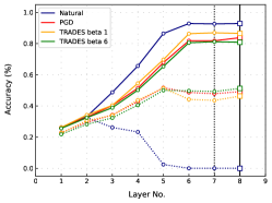
(a) CIFAR10-ResNet-18

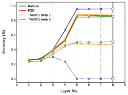
(b) CIFAR10-WideResNet-36-10

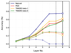
(c) CIFAR100-ResNet-18

Figure 2. Accuracy of clean samples (solid lines) and PGD adversarial examples (dashed lines) on each neural network layer with different training methods. Vertical dashed lines indicate the penultimate layer, and vertical solid lines indicate the logit layer. For layers before the logit layer (i.e., the last layer), the accuracy indicates the accuracy of the $f_{\text{1-nn}}$. The accuracy of the logit layer is identical to the classification accuracy of the network. PGD examples were generated from clean test samples with $\epsilon=8/255$, step size $\alpha=2/255$, and attack iteration $N=20$. We measured the $l_{1}$ distance between the layer output of a test sample and those of train samples.

We observed the relationship between the alignment in the feature representation of hidden layers and the classification accuracy. Figure 2 describes the accuracy of each neural network layer for test inputs. The accuracy of layers before the penultimate layer denotes the accuracy of the 1-nearest neighbor $f_{\text{1-nn}}$ that uses the output of each layer. We identified consistent results for all datasets, architectures, and training methods. The accuracy of the first layer in Figure 2 cannot discriminate between clean samples and adversarial examples. As the layer went deeper, the accuracy converged toward that of the logit layer: the accuracy of the penultimate layer was the most similar to the logit layer. These results imply that the penultimate layer output is the most influential in the linear classifier.

Table 3. Accordance rate of training methods for ResNet-18 on CIFAR10 and CIFAR100. The accordance rate is the ratio of samples the majority of whose k-nearest neighbors in feature space have the same class as the predicted class from the neural network for the samples. We used $\epsilon=8/255$, step size $\alpha=2/255$, and attack iteration $N=20$ for PGD attack. We used the $l_{1}$ distance between the penultimate layer output of a test sample and those of training samples.

Training Method	Clean (%)		PGD(%)
	k=1	k=100	k=1	k=100
CIFAR10 Dataset
Cross-entropy	96.54	98.39	99.99	99.99
PGD AT (Madry et al., 2017)	76.56	87.74	67.95	83.04
AdvCL (Fan et al., 2021)	84.46	89.46	76.16	82.98
AFA (ours)	95.34	96.07	84.43	87.95
CIFAR100 Dataset
Cross-entropy	74.83	81.02	96.27	98.03
PGD AT (Madry et al., 2017)	48.18	63.73	40.65	60.19
AdvCL (Fan et al., 2021)	53.93	69.81	46.49	65.82
AFA (ours)	70.72	76.12	53.00	63.62

3.5. Correlation between Misaligned Classes and Misclassified Classes

We further observe whether a class whose manifold the feature of a sample is located affects the prediction of the linear classifier. We deploy a k-nearest neighbor (k-NN) classifier that uses the outputs of the feature extractor as an input. We identify whether the predicted class of the linear classifier corresponds with the majority of k-nearest neighbors. We set k to 1 and 100.

The accordance rate in Table 3 describes the ratio of samples that the neural network and k-NN classifier yield the same class. With natural cross-entropy, predictions of the network and the k-NN classifier agreed for most samples regardless of the misclassification. One possible reason is that natural training uses only clean samples to learn feature distribution, so the feature representation of the network becomes monotonous. This result indicates that the manifold where the feature of a sample locates is significantly utilized for the decision of the linear classifier. Adversarial training methods showed lower accordance rates than natural training. Nevertheless, their accordance rates are still high, implying that linear classifiers from adversarial training depend on the manifold in the feature space. We also see that our method yields the highest accordance rates among adversarial training methods. From our method, samples are better aligned along their classes in the feature space, and the uncertainty of the linear classifier is mitigated.

4. Adversarial Feature Alignment

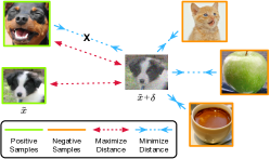
(a) Inner optimization step

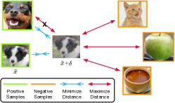
(b) Outer optimization step

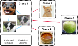
(c) After training

Figure 3. Overview of Adversarial Feature Alignment (AFA): AFA incorporates inner and outer optimization steps in each training epoch. (a) In the inner step, an adversarial example $\tilde{x}+\delta$ is generated to maximize the AFA adversarial loss, optimizing feature vector distances from both positive and negative examples. (b) The feature extractor $g$ is then updated to minimize the feature vector distance from positive examples and maximize it from negatives. (c) Post-AFA training, class samples are efficiently clustered into their respective classes, optimizing both intra-cluster closeness and inter-cluster separation.

In this section, we propose Adversarial Feature Alignment (AFA), a new robust training method for the feature extractor $g$ of $f_{\text{dnn}}$. We define a new adversarial contrastive loss in a fully-supervised manner and solve the min-max optimization problem that targets the loss, as illustrated in Figure 3. AFA effectively solves the robustness-accuracy tradeoff because it finds the worst-case sample that degrades alignment and optimizes it. In this respect, we revisit the existing contrastive loss function in §4.1 and discuss principles of a new loss function for the effectiveness of AFA in §4.2. We design AFA loss function in §4.3 and new optimization strategy of AFA in §4.4.

4.1. Revisiting Contrastive Loss Function

Contrastive learning is a training method to pretrain the feature extractor of a DNN. The objective is minimizing the feature distance between an anchor sample and its positive samples and maximizing the feature distance between the anchor and its negatives. Let $X=\{x_{1},x_{2},...,x_{n}\}$ be an input batch, and $Y=\{y_{1},y_{2},...,y_{n}\}$ be its corresponding class label batch. The supervised contrastive loss is measured over a multiview batch. In this paper, we consider the multiview batch $\tilde{X}=\{\tilde{x}_{1},\tilde{x}_{2},...,\tilde{x}_{kn}\}$, which is the $k$-fold augmentation of $X$, where $\{\tilde{x}_{k(i-1)+1},...,\tilde{x}_{ki}\}$ are randomly transformed images of $x_{i}$. $Y$ is also augmented to $\tilde{Y}=\{\tilde{y}_{1},\tilde{y}_{2},...,\tilde{y}_{kn}\}$, where $\tilde{y}_{k(i-1)+1}=...=\tilde{y}_{ki}=y_{i}$.

Self-supervised contrastive loss function. Self-supervised contrastive learning (Chen et al., 2020a) does not use the class label. Instead, it labels the augmentations of the same original sample as the anchor as positive and the remaining samples in the batch as negative. Samples derived from original samples different than the anchor are labeled negative, even though their class is the same as the anchor. The self-supervised contrastive loss $\mathcal{L}_{self}$ is formulated as follows:

(3) $$\mathcal{L}_{self}=\sum_{i=1}^{kn}\frac{-1}{|P_{self}(\tilde{x}_{i})|}\sum_{\tilde{x}_{p}\in P_{self}(\tilde{x}_{i})}\log\frac{e^{z_{\tilde{x}_{i}}\cdot z_{\tilde{x}_{p}}/\tau}}{\underset{a\in A(\tilde{x}_{i})}{\sum}e^{z_{\tilde{x}_{i}}\cdot z_{a}/\tau}}.$$

In Eq. 3, $z_{x}=\phi(g(x))\in\mathbb{R}^{D_{P}}$ is a normalized feature embedding of $g(x)$ by the projection layer $\phi$. $\phi$ is a multi-layer perceptron and is used only for the pre-training phase. $A(\tilde{x}_{i})=\tilde{X}\ \backslash\ \{\tilde{x}_{i}\}$ is the contrastive view of the anchor sample $\tilde{x}_{i}$ and incorporates positive and negative samples of $\tilde{x}_{i}$. $P_{self}(\tilde{x}_{i})$ is a set of positive samples of $\tilde{x}_{i}$. It consists of samples derived from the original sample same as $\tilde{x}_{i}$. Negative samples of $\tilde{x}_{i}$ in $\mathcal{L}_{self}$ are $A(\tilde{x}_{i})\backslash P_{self}(\tilde{x}_{i})$. The inner dot product calculates the distance of feature embeddings between two samples. $\tau$ is a temperature to regularize inner dot products. In summary, for each training sample, the loss function in Eq. 3 calculates the feature product with the positives that should be maximized in the numerator and the feature product with the negatives that should be minimized in the denominator.

Supervised contrastive loss function. It is known that the fully-supervised contrastive learning (Khosla et al., 2020) performs better than the self-supervised one (Chen et al., 2020a) in general. This approach has a different criterion on positive and negative samples from the self-supervised one: all samples in the same class as the anchor are positive and samples in the other classes are negative. The supervised contrastive loss $\mathcal{L}_{sup}$ is formulated as follows:

(4) $$\mathcal{L}_{sup}=\sum_{i=1}^{kn}\frac{-1}{|P_{sup}(\tilde{x}_{i})|}\sum_{\tilde{x}_{p}\in P_{sup}(\tilde{x}_{i})}\log\frac{e^{z_{\tilde{x}_{i}}\cdot z_{\tilde{x}_{p}}/\tau}}{\underset{a\in A(\tilde{x}_{i})}{\sum}e^{z_{\tilde{x}_{i}}\cdot z_{a}/\tau}}.$$

Eq. 4 and Eq. 3 are almost the same but the difference is the term for a positive set. The positive set in Eq. 4 is $P(\tilde{x}_{i}):=\{\tilde{x}_{p}\in A(\tilde{x}_{i}):\tilde{y}_{p}=\tilde{y}_{i}\}$. $L_{sup}$ of Eq. 4 is the same as $L^{sup}_{out}$ of (Khosla et al., 2020). $L^{SCL}_{out}$, whose summation over positives of an anchor is outside the log, had better performance than $L^{sup}_{in}$ in that work.

4.2. Principles for Adversarial Feature Alignment

Adversarial training over contrastive loss is necessary. Vanilla contrastive learning is the simple alignment of clean samples, so the contrastive loss does not address potentially misaligned samples, even if the clean samples can be aligned in feature space. This means that the model is overfitted to the manifold of clean samples and is vulnerable to adversarial examples that force misalignment. Therefore, we need to maximize the risk of feature misalignment during the learning process.

Supervised contrastive loss better than self-supervised one. The inner step of the self-supervised loss has difficulty generating the adversarial example that maximizes the risk of feature misalignment. For example, the self-supervised loss forces the adversarial example to move closer toward the samples in the same class, as shown in the blue line marked with ’X’ in Figure 3(a). This adversarial example is not the worst-case because it cannot widen the cluster of its class (i.e., maximize the radius of the manifold of the class). In the outer step, the self-supervised loss separates even samples in the same class, as shown in the red line marked with ’X’ in Figure 3(b), which may hinder the clustering of the class.

Effective positive and negative mining. The contrastive view $A$ of the adversarial example $\tilde{x}_{i}$ as an anchor is filled with other anchors from the batch in previous adversarial contrastive learning methods, meaning that samples in the contrastive view are adversarial. Therefore, previous methods cannot guide a direction toward the correct class manifold for the adversarial anchor. Adversarial feature alignment requires effective positive and negative mining of benign samples to provide the right direction toward the correct class manifold.

4.3. AFA Loss Function

We design a new loss function for AFA the principles in Section 4.2. AFA assumes an adversary who tries to push apart the feature of an anchor from its positives (i.e., samples in the same class) and moves the feature of the anchor towards its negatives. The worst-case adversarial example in AFA settles into the center of the manifold of a different class different from the example. The adversary’s objective corresponds with maximizing the AFA loss function $L_{AFA}$ that can be formulated as follows:

(5) $$\mathcal{L}_{AFA}=\sum_{i=1}^{kn}\frac{-1}{|P_{AFA}(\tilde{x}_{i}^{\prime})|}\sum_{\tilde{x}_{p}\in P_{AFA}(\tilde{x}_{i}^{\prime})}\log\frac{e^{z_{\tilde{x}_{i}^{\prime}}\cdot z_{\tilde{x}_{p}}/\tau}}{\underset{a\in A_{AFA}(\tilde{x}_{i}^{\prime})}{\sum}e^{z_{\tilde{x}_{i}^{\prime}}\cdot z_{a}/\tau}}.$$

$L_{AFA}$ in Eq. 5 is different from $L_{sup}$ in Eq. 4 in various views. The anchor view is $\tilde{X}^{\prime}=\tilde{X}+\delta$, such that an anchor $\tilde{x}_{i}^{\prime}=\tilde{x}_{i}+\delta_{i}$ in $\tilde{X}^{\prime}$ is an adversarial view of $\tilde{x}_{i}$ in $\tilde{X}$ with the worst-case perturbation $\delta_{i}$. The contrastive view is $A_{AFA}(\tilde{x}_{i}^{\prime}):=\tilde{X}$. In other words, positive and negative samples are selected from benign samples. Any other anchor than $\tilde{x}_{i}^{\prime}$ is not included in the contrastive view $A_{AFA}(\tilde{x}_{i}^{\prime})$ in $L_{AFA}$, while each anchor constructs a contrastive view in $L_{sup}$. The positive samples in AFA loss is $P_{AFA}(\tilde{x}_{i}^{\prime}):=\{\tilde{x}_{p}\in A_{AFA}(\tilde{x}_{i}):\tilde{y}_{p}=\tilde{y}_{i}\}$.

Our loss function 1) is compatible to adversarial training, 2) is based on the supervised contrastive learning, and 3) provides a direction toward correct data manifold of classes. AFA loss function has the effectiveness of hard positive and hard negative mining because the feature of an adversarial example shifts along the manifold of benign samples whose features are easier to align. Further, we have a different perspective from self-supervised adversarial contrastive learning methods (Kim et al., 2020; Jiang et al., 2020; Ho and Nvasconcelos, 2020; Fan et al., 2021): we recruit all samples with the same class as the anchor from the clean multiview batch for positives.

4.4. Training Strategy of AFA

Baseline optimization. The optimization algorithm of AFA is similar to TRADES (Zhang et al., 2019) in that both simultaneously minimize natural and adversarial risks during the outer optimization. The optimization problem of TRADES is as follows:

(6) $$\text{{TRADES}}:=\underset{f}{\text{min}}\ \mathbb{E}\biggl{\{}\mathcal{L}_{CE}(f(X)Y)+\underset{X^{{}^{\prime}}\in\mathbb{B}(X,\epsilon)}{\text{max}}\beta\cdot\mathcal{L}_{KL}(f(X)f(X^{{}^{\prime}}))\biggl{\}}.$$

$\mathcal{L}_{KL}$ in Eq. 6 is KL divergence loss, and $\beta$ is a coefficient to regularize the importance of adversarial loss. $X^{{}^{\prime}}$ is a set of adversarial examples that maximizes the inner loss function. Based on the AFA loss function of Eq. 5 and Eq. 6, we define the baseline optimization algorithm of AFA as follows:

(7) $$\text{{AFA}}:=\underset{\theta_{g}}{\min}\ \mathbb{E}_{(x,y)\sim\mathcal{D}}\ \{\lambda_{1}\mathcal{L}_{sup}+\underset{||\delta||\leq\epsilon}{\max}\lambda_{2}\mathcal{L}_{AFA}\}.$$

AFA performs the inner optimization in Eq. 7 by maximizing the loss $\mathcal{L}_{AFA}$ in Eq. 5 through the projected gradient descent (Madry et al., 2017). This process is identical to finding the worst-case sample farthest from its true class and closest to its other classes, given the current distribution of feature space (see Figure 3(a)). While minimizing the AFA loss, the feature vector of the worst-case sample is relocated to the vicinity of clean samples in its true class (see Figure 3(b)). AFA embodies Theorem 3.5 in action, as it concurrently conducts clustering and separation throughout training. We believe that minimizing vanilla supervised contrastive loss $L_{sup}$ is helpful because feature values of well-aligned training samples are a reliable label for the AFA loss where ground-truth labels are not given in the feature space.

The coefficient $\lambda$ regularizes the influences of $L_{sup}$ and $L_{AFA}$. Eq. 7 is identical to the vanilla supervised contrastive learning (Khosla et al., 2020) when $\lambda_{2}=0$. On the other hand, Eq. 7 targets only the AFA loss when $\lambda_{1}=0$. Through the ablation study in Appendix E.2 and Table 15, we set $\lambda_{1}=1$ and $\lambda_{2}=2$ for the baseline AFA. Based on the result of Table 16, we apply the 3-fold augmentation to the baseline AFA: for each original image, two derivatives are randomly transformed, and the other is preserved.

Pre-training with AFA. The most basic training method with AFA, similar to other contrastive learning techniques, involves pre-training followed by fine-tuning. In this case, AFA optimization denoted by Eq. 7 is used solely to pre-train a neural network’s feature extractor. Subsequently, traditional adversarial training methods that utilize the loss function of the output layer are employed to fine-tune either the neural network’s linear classifier or its entire parameters.

Joint optimization method. AFA optimization impacts only the feature extractor, not the linear classifier. Therefore, it is possible to use AFA in conjunction with other adversarial training methods. Algorithm 1 describes the procedure of our joint optimization that combines AFA with TRADES. We use original inputs in a training batch to optimize TRADES loss and augmented inputs to optimize AFA loss. In the inner step, we individually generate adversarial examples that maximize the AFA loss denoted by Eq.5 and the KL loss from TRADES. In the outer step, we use these adversarial examples to minimize both Eq.7 and Eq. 6 simultaneously. Due to the considerably higher AFA loss values compared to TRADES loss values, we use the TRADES loss as is to update the network parameter but regularize the AFA loss value by a factor of 0.1. This approach can also be combined with other training methods, not just TRADES.

Algorithm 1 Joint optimization of AFA and TRADES

1:Input: Neural network $f$ that consists of feature extractor $g$ and linear classifier $h$

2:Input: Network parameters $\theta_{f},\theta_{g},\theta_{h}$

3:Input: Training batch $\tilde{X}$, class label $Y$, perturbation size $\epsilon$

4:Output: Updated network parameters

5:$\tilde{X}_{TRADES},\tilde{X}_{AFA}$ $\leftarrow$ Separate($\tilde{X}$) $\triangleright$ Separate the batch into original inputs and augmented inputs.

6:// Inner maximization phase

7:$\delta_{AFA},\delta_{TRADES}$ $\leftarrow$ Uniform($-\epsilon,\epsilon$) $\triangleright$ Initialize adversarial perturbations.

8:$\delta_{AFA}$ $\leftarrow$ $\underset{\delta_{AFA}}{\text{max}}\mathcal{L}_{AFA}(\theta_{g},\tilde{X}_{AFA},Y,\delta_{AFA})$ $\triangleright$ Derive adversarial perturbation maximizing AFA loss for the augmented inputs.

9:$\delta_{TRADES}$ $\leftarrow$ $\underset{\delta_{TRADES}}{\text{max}}\mathcal{L}_{KL}(\theta_{f},\tilde{X}_{TRADES},\delta_{TRADES})$ $\triangleright$ Derive adversarial perturbation maximizing TRADES loss for the original inputs.

10:// Outer minimization phase

11:$\mathcal{L}_{AFA}$ $\leftarrow$ $\lambda_{1}\mathcal{L}_{sup}(\tilde{X}_{AFA},Y)+\lambda_{2}\mathcal{L}_{AFA}(\tilde{X}_{AFA},Y,\delta_{AFA})$ $\triangleright$ Measure AFA training loss.

12:$\mathcal{L}_{TRADES}$ $\leftarrow$ $\mathcal{L}_{CE}(f(\tilde{X}_{TRADES})Y)+\beta\cdot\mathcal{L}_{KL}(f(\tilde{X}_{TRADES})f(\tilde{X}_{TRADES}+\delta_{TRADES}))$ $\triangleright$ Measure TRADES training loss.

13:$\mathcal{L}_{joint}$ $\leftarrow$ $\mathcal{L}_{TRADES}+0.1\cdot\mathcal{L}_{AFA}$ $\triangleright$ Derive the final training loss

14:$\theta_{f}$ $\leftarrow$ Update($\theta_{f}$, $\mathcal{L}_{joint}$) $\triangleright$ Update parameters with the joint loss

5. Evaluation

Table 4. Clean and robust accuracy of different training methods for ResNet-18. The best results among adversarial training methods are highlighted in bold. The attack parameters for PGD are the same as Table 2. AA denotes AutoAttack (Croce and Hein, 2020) which ensembles multiple parameter-free attacks for more reliable robustness verification.

Training Method	CIFAR10 (%)			CIFAR100 (%)
	Clean	PGD	AA	Clean	PGD	AA
Natural Training Methods
Cross-entropy	92.87	0	0	75.05	0	0.02
SupCon (Khosla et al., 2020)	93.44	17.90	0.02	65.99	0.02	0.08
Adversarial Training Methods
PGD AT (Madry et al., 2017)	83.77	49.18	38.15	57.69	25.78	14.57
TRADES $\beta$=$1$ (Zhang et al., 2019)	86.49	46.29	34.70	62.61	21.34	13.64
TRADES $\beta$=$6$ (Zhang et al., 2019)	80.84	51.23	40.03	57.04	28.25	15.58
AWP (Wu et al., 2020)	80.40	54.71	49.57	-	-	-
Adversarial Contrastive Learning Methods
AdvCL (Fan et al., 2021)	80.24	53.93	41.08	58.4	29.86	16.83
+ A-InfoNCE (Yu et al., 2022)	83.78	54.36	41.32	59.16	30.47	17.23
AFA (ours)	91.01	57.77	52.05	66.14	29.97	19.02

In this section, we evaluate the performance of our method, Adversarial Feature Alignment (AFA), from various perspectives. We evaluate the baseline performance of AFA as an adversarial contrastive learning method, and verify our improvements in accuracy to clean samples and adversarial examples (§5.1). We observe how well aligned the feature space learned by our robust training method (§5.2). In the ablation study, we evaluate the performance change of adversarial feature alignment concerning training settings (§5.3). We apply the joint approach of AFA to the state-of-the-art adversarial training method and benchmark the performance of AFA (§5.4). The experimental settings for AFA and other training methods are described in the Appendix C.

5.1. Baseline Performance of AFA

Tradeoff between robustness and accuracy. Table 4 describes the accuracy of training methods to clean samples and adversarial examples. We consider cross-entropy and vanilla supervised contrastive learning (SupCon) (Khosla et al., 2020) for natural training methods. For adversarial training methods, we consider PGD AT (Madry et al., 2017), TRADES (Zhang et al., 2019), and adversarial weight perturbation (AWP) (Wu et al., 2020). We also consider AdvCL (Fan et al., 2021) and A-InfoNCE (Yu et al., 2022), the state-of-the-art adversarial contrastive learning schemes.

Natural training methods achieved the highest accuracy to clean samples but misclassified most adversarial examples for both datasets. Adversarial training methods improved robust accuracy compared to natural training, but they underwent a drop in clean accuracy. AdvCL and A-InfoNCE yielded higher robust accuracy than PGD and TRADES, demonstrating the effectiveness of pre-training with adversarial contrastive learning. AWP, the more recent work than TRADES, aims at robustness generalization and showed the highest robust accuracy among previous methods. However, none of the adversarial training methods showed the best accuracies for both clean samples and adversarial examples.

AFA resulted in the best performance among all adversarial training methods in CIFAR10 and CIFAR100. The robust accuracy of AFA on CIFAR10 was the highest for all adversarial attacks. The robust accuracy of AFA to PGD on CIFAR100 was slightly lower than A-InfoNCE. However, AFA showed the highest accuracies for AutoAttack, a parameter-free attack, implying that our methods are robust against unlearned types of attacks. We also see that AFA’s clean accuracy significantly improved from previous adversarial training methods. We cost only a 2.43%p drop in clean accuracy compared to vanilla SupCon, and our clean accuracy was even 7.23%p and 4.52%p higher than A-InfoNCE and TRADES $\beta=1$ on CIFAR10, respectively. Furthermore, the clean accuracy of AFA was only 8.91%p lower than the cross entropy and even 0.15%p higher than the vanilla SupCon on CIFAR100. We identified from this result that AFA improves the tradeoff between robustness and accuracy.

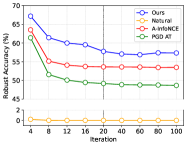
(a) Attack Iteration

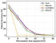
(b) Perturbation Size

Figure 4. Robust accuracy of training methods against varying attack strength. (a) We set $\epsilon=8/255$ and $\alpha=2/255$ for the PGD attack while changing the number of attack iterations $N$. (b) We set the number of iterations $N=20$ and $\alpha=\epsilon/4$ while changing the perturbation size $\epsilon$. The target model is ResNet-18 and experimented dataset is CIFAR10.

Robustness against stronger attack. To evaluate the performance of AFA against a more powerful attack, we consider two cases: a PGD adversary who changes the number of attack iterations with fixed perturbation size and another PGD adversary who changes perturbation size with fixed attack iterations. In Figure 4(a), the increase of attack iteration marginally reduced the robust accuracy for other methods. Our method showed the best performance than other methods for all attack iterations and even improved the accuracy against more attack iterations. In Figure 4(b), the increase of perturbation size resulted in a meaningful impact on the robustness. All training methods including our method failed to avoid the reduction in the robust accuracy. AFA exhibited the best performance within the permissible perturbation size, but showed slightly lower robust accuracy than A-InfoNCE when the perturbation was sufficiently large. This result leaves future work for AFA in resolving feature misalignment that occurs with larger distortions in the input space.

Table 5. Accuracy (%) of different training methods on additional scenarios. We could not evaluate A-InfoNCE in restricted ImageNet because of its complexity: it took more than few weeks for pretraining in our settings.

	CIFAR100		Restricted ImageNet
	ResNet-50		ResNet-18
Method	Clean	PGD	Clean	PGD
TRADES $\beta$=1 (Zhang et al., 2019)	61.76	23.08	90.34	83.04
TRADES $\beta$=6 (Zhang et al., 2019)	57.17	28.92	89.56	84.27
A-InfoNCE (Yu et al., 2022)	60.40	31.47	-	-
AFA (Ours)	68.50	41.28	90.55	84.79

Performance of AFA on different scenarios. To evaluate the generalizability of our method, we conducted experiments on additional scenarios. We verified TRADES, A-InfoNCE, and AFA for ResNet-50, a more extensive model than ResNet-18, on CIFAR100. We also evaluated these methods on restricted ImageNet, the larger dataset with more samples and higher resolution. We aimed to validate a dataset distinct from CIFAR10 and CIFAR100. Due to the computational demands of the original ImageNet, we opted for the widely-used restricted ImageNet as a substitute. As seen in the left two columns of Table 5, all methods improved their CIFAR100 accuracies from those on ResNet-18. Nevertheless, AFA achieved remarkable improvements compared to other training methods and still demonstrates the highest accuracies. The robust accuracy of AFA against PGD was 9.81%p higher than that of A-InfoNCE on CIFAR100 with ResNet-50. This indicates the beneficial impact of model capacity on the feature alignment task in complex datasets. In the right two columns of the Table, when using the ResNet-18 model on the Restricted ImageNet dataset, AFA showed better performance in terms of both robustness and accuracy than TRADES, implying its generalizability.

5.2. Feature Alignment and Generalization

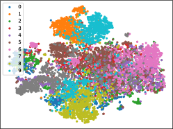
(a) PGD Training (Madry et al., 2017)

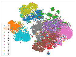
(b) AdvCL (Fan et al., 2021)

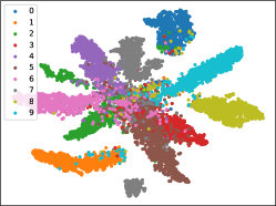
(c) Adversarial Feature Alignment (Ours)

Figure 5. t-SNE visualization of feature spaces represented by adversarial training methods on CIFAR10. While PGD and AdvCL result in widespread feature spaces, our adversarial feature alignment method separates classes more distinctly.

Visualization of feature space. Figure 5 describes that AFA, in a supervised manner, led to a remarkable alignment in the feature topology with the same network capacity. We identified that the feature space was not clearly separated and clustered by other methods. Although some samples overlap in the center for AFA, the remaining ones are more clearly separated from other classes. We chose CIFAR10 as a representative result due to its balanced number of samples and classes. We expect that the visualization for CIFAR100, which had lower accuracy, might be less clear, while restricted ImageNet, with its higher accuracy, should produce a distinct feature space similar to CIFAR10.

Table 6. Analysis of separation and alignment in the penultimate layer output of ResNet-18 models, trained by various methods, on CIFAR10. ’Clean’ column compares training with clean test samples, while ’PGD’ column contrasts training samples with PGD test examples, using the same attack parameters as in Table 2.

	Min Separation		Max Clustering
Training Method	Clean	PGD	Clean	PGD
Cross-entropy based Methods
Cross-entropy	1.358	0.938	23.496	25.067
PGD AT (Madry et al., 2017)	0.970	1.480	22.659	24.632
TRADES $\beta=1$ (Zhang et al., 2019)	1.789	1.608	21.980	23.352
TRADES $\beta=6$ (Zhang et al., 2019)	1.516	1.460	22.743	23.355
Contrastive Learning Methods
SupCon (Khosla et al., 2020)	3.547	1.447	19.789	20.919
AdvCL (Fan et al., 2021)	2.094	1.755	19.989	20.261
+ A-InfoNCE (Yu et al., 2022)	1.790	1.526	19.758	20.486
AFA (Ours)	3.674	3.260	18.095	19.021

Alignment in feature space. We evaluate whether AFA improves the alignment of feature space by increasing the separation factor and reducing the clustering factor. Table 6 describes the minimum separation and maximum clustering factors of training methods. Adversarial examples worsen the alignment than clean test samples for all training methods. Contrastive learning-based methods generally showed better performance in alignment than cross-entropy-based methods: The distance between different classes was further, and the maximum radius of one class was shorter. The separation of clean samples through the vanilla SupCon was improved remarkably, that of adversarial examples was worse than cross-entropy-based robust training methods. The reason is that the feature alignment that only targets clean samples cannot generalize features of adversarial examples. AdvCL and A-InfoNCE, which use an instance-wise loss function, also showed no significant improvement in separation. On the other hand, AFA performed best in separation and clustering for all types of samples. We further verified the generalization performance of AFA through local Lipschitzness in Appendix E.1 and Table 14. The results show that AFA demonstrates its robustness against adversarial examples that worsen local Lipschitzness.

5.3. Ablation Study

Table 7. Accuracy comparison of different supervised contrastive learning optimization methods on CIFAR10 and CIFAR100 using ResNet-18. The first row shows results using a joint loss function without optimization of AFA loss (Eq. 8). The second and third rows depict pre-training with Eqs. 9 and 7, followed by adversarial linear fine-tuning.

Optimization	CIFAR10 (%)		CIFAR100 (%)
Method	Clean	PGD	Clean	PGD
Eq. 8	84.46	41.42	57.45	22.42
Eq. 9	87.6	43.04	59.25	28.74
Eq. 7 (AFA, ours)	91.01	57.77	66.14	29.97

Comparison with other optimizations. We identify the necessity of AFA for robustness-accuracy tradeoff instead of other variations of supervised contrastive learning. We trained the neural network using two optimization strategies and compared the performance with our method in Table 7.

Similar to the joint approach of AFA, one can consider a loss function that combines supervised contrastive loss and adversarial cross-entropy loss. Following (Bui et al., 2021), we define Eq 8:

(8) $$\underset{\theta}{\min}\ \mathbb{E}_{(x,y)\sim\mathcal{D}}\{\mathcal{L}_{SCL}+\underset{||\delta||\leq\epsilon}{\max}\mathcal{L}_{CE}(x+\delta,y;\theta)\}.$$

Eq. 8 first generates an adversarial example with maximized cross-entropy loss and then minimizes the joint loss function in each training epoch. The difference between AFA and Eq. 8 is the inner maximization of AFA loss. For the first row in Table 7, we trained an entire network with Eq. 8 from the scratch for 100 epochs. We can also consider another strategy that does not take hard positive and negative mining. We define Eq. 9:

(9) $$\underset{\theta_{g}}{\min}\ \mathbb{E}_{(x,y)\sim\mathcal{D}}\ \underset{||\delta||\leq\epsilon}{\max}\mathcal{L}_{SCL}$$

where the min-max problem is solved with vanilla SupCon loss of only adversarial examples. For this strategy, we performed pre-training and fine-tuning with our baseline settings.

Results in Table 7 show that our strategy is the most accurate to clean and adversarial samples for both datasets. Eq. 9 yields better accuracies than Eq. 8, indicating that pre-training with SupCon loss is quite effective for accuracy and robustness. We empirically found that Eq. 8 converges in the intermediate epoch. However, maximizing vanilla SupCon loss considerably decreased the accuracy compared to our strategy.

5.4. Improving Adversarial Training via AFA

In this section, we combine AFA with state-of-the-art adversarial training methods to achieve enhanced performance. Recent studies have shown that data augmentation based on generated models, especially the denoising diffusion probabilistic model (DDPM) (Ho et al., 2020), is helpful in adversarial training (Gowal et al., 2021; Rebuffi et al., 2021; Wang et al., 2023). Notably, Wang et al. (Wang et al., 2023) achieved top-1 performance on RobustBench in terms of accuracy for clean samples and AutoAttack by utilizing a more recent diffusion model, the elucidating diffusion model (EDM) (Karras et al., 2022). They composed training batches with original and generated data, setting the original-to-generated ratio at 0.3. Labels for the original and generated data were derived respectively from the dataset’s ground truth and the predictions of a pre-trained non-robust model.

Since their focus was on data augmentation, they continued to use TRADES as the training loss function. Therefore, it is expected that replacing TRADES with AFA, which had outperformed TRADES in baseline experiments, would further enhance performance. We employed 1 million samples of data generated by EDM, as per the basic setup of Wang et al. (Wang et al., 2023), for training the WideResNet-28-10 model. We adopted the joint optimization of AFA and TRADES of Section 4.4 with $\lambda_{1}=1$, $\lambda_{2}=5$, and $\beta=5$, respectively.

Table 8. Comparison with the latest adversarial training technique (Wang et al., 2023) on CIFAR10 using WideResNet-28-10. Note: ^∗ indicates training samples generated via a diffusion model.

	Settings			Accuracy (%)
Method	Generated∗	Batch	Epoch	Clean	PGD	AA
Wang et al.  (Wang et al., 2023)	1M	512	400	90.91	64.18	63.07
	1M	1024	800	91.18	65.12	62.39
Joint AFA	1M	512	400	91.79	64.31	62.94

Table 8 presents the performance comparison between the pure approach of Wang et al. (Wang et al., 2023) and the approach that additionally combines AFA. For the same batch size and training epochs, joint AFA demonstrated slightly lower accuracy against AutoAttack compared to Wang et al. (Wang et al., 2023), but it showed higher accuracy against PGD adversarial examples. Moreover, joint AFA improved the accuracy on clean samples by 0.88 percentage points over Wang et al. Under the same conditions, AFA exhibited higher accuracy than Wang et al. (Wang et al., 2023), who applied a batch size of 1024 and training epochs of 800, for both clean samples and AutoAttack.

Wang et al. also conducted experiments on a larger model, the WRN-70-16 with 267M parameters, in comparison to the WRN-28-10, which has 36M parameters. Although our performance on the WRN-28-10 was somewhat lower than their results on the WRN-70-16, we demonstrated comparable performance with the same model size, suggesting potential generalization to that model. Due to our limited computing resources, further experiments with more generated data and model parameters are left for future work.

6. Discussion

Implication of our work. The prevailing understanding is that a Lipschitz-bounded linear classifier, due to its large margin, yields better generalization performance (von Luxburg and Bousquet, 2004; Xu et al., 2009). Previously, it was believed that sufficient separability in the dataset’s input space is key for model generalization (Yang et al., 2020). However, our research challenges this notion by showing that even with distinguishable classes, the distance metric in the input space can hinder generalization due to greater distances among same-class samples. We advocate for the generalization of the ’real’ linear classifier in DNNs through the alignment of the feature space, as opposed to the static input space. Our findings indicate that low accuracy of a 1-NN classifier in the feature space suggests considerable overlap in feature distributions between classes, compromising the margin. This misalignment can lead to a reduced margin in the DNN’s logit layer, increasing misclassifications. Adversarial Feature Alignment (AFA), by directly targeting feature misalignment, can enhance the margin for the linear classifier more effectively than other methods, thereby improving classification generalization.

Suitable fine-tuning method of AFA pretraining. Contrastive learning fine-tuning can be broadly classified into four methods: Standard Linear Fine-tuning (SLF), Adversarial Linear Fine-tuning (ALF), Standard Full Fine-tuning (SFF), and Adversarial Full Fine-tuning (AFF). Standard methods focus on minimizing loss on clean samples without generating adversarial examples during training, whereas adversarial methods create and minimize loss on adversarial examples. Linear methods only update the linear classifier’s parameters, keeping the feature extractor constant, while full methods update all DNN layer parameters. In this paper, we apply ALF to AFA, unlike other adversarial contrastive learning methods that use AFF. We found that AFF, a full fine-tuning method, can degrade the feature extractor. Although the model performance using AFF after AFA pretraining is similar to existing methods, our primary interest lies in pretraining the feature extractor. Developing a novel fine-tuning method suited to AFA is left for future research.

Adaptive attacker to our approach. An adaptive attacker, armed with white-box knowledge of the model, dataset, and training method, aims to compromise AFA by manipulating input images to misalign class features, causing misclassification. This strategy involves using gradients that maximize AFA loss, mirroring AFA’s internal optimization process. We tested this attack on a model trained with baseline AFA using 20-PGD iterations and noted a success rate of 28.99%, lower than the 42.23% achieved by the original PGD. These results indicate that AFA maintains robustness against such adaptive attacks.

7. Related Work

Adversarial defense and robust training. Adversarial training (Goodfellow et al., 2014; Bai et al., 2021) is a method used alongside techniques like adversarial detection (Grosse et al., 2017; Freitas et al., 2020; Huang et al., 2019; Li and Li, 2017; Ma et al., 2018; Lee et al., 2018; Liu et al., 2019; Lu et al., 2017) and denoising (Liao et al., 2018; Samangouei et al., 2018; Meng and Chen, 2017; Das et al., 2018; Cho et al., 2020; Guo et al., 2018; Abusnaina et al., 2021) as one of the most effective methods for enhancing neural network robustness against adversarial examples. The core idea of adversarial training is to learn from adversarial examples created with worst-case perturbations (Goodfellow et al., 2014). This approach is conceptualized as a saddle point problem (Madry et al., 2017), where the inner maximization and outer minimization problems are jointly optimized for the cross-entropy loss, with methods like projected gradient descent used to maximize this loss (Madry et al., 2017). The following works have built upon this foundation (Madry et al., 2017), addressing issues like computational complexity (Shafahi et al., 2019; Wong et al., 2020) and overfitting (Rice et al., 2020).

Robustness-accuracy tradeoff. Several studies have highlighted an inherent tradeoff between robustness and accuracy in neural networks (Tsipras et al., 2018; Zhang et al., 2019; Raghunathan et al., 2019). This tradeoff is partly attributed to the conflicting goals of natural and robustness-focused training. Robust generalization (Rade and Moosavi-Dezfooli, 2021; Raghunathan et al., 2020; Chen et al., 2020c; Wu et al., 2021, 2020) has become a key area of focus to address this issue. For instance, a network’s robustness can be certified over a radius $\epsilon$ by estimating its Lipschitz bounds (Yang et al., 2020; Lee et al., 2020; Leino et al., 2021). While Yang et al. (Yang et al., 2020) suggested that a low local Lipschitz bounded classifier can resolve the tradeoff in separated datasets, our research in Section 3 indicates that an accurate classifier requires not just separation, but also alignment within the dataset. Our empirical findings demonstrate that datasets which are separated but not aligned are prone to misclassifications.

To address the robustness-accuracy tradeoff, various strategies have been proposed. TRADES (Zhang et al., 2019) regularizes both standard and robust errors. Wang et al. (Wang et al., 2020) developed a surrogate loss function facilitating misclassification-aware regularization. Raghunathan et al.’s robust self-training leverages additional unlabeled data (Raghunathan et al., 2020). Zhang et al.’s approach adjusts the loss function weight based on the distance from the decision boundary (Zhang et al., 2021b). Helper-based adversarial training reduces the excessive margin in decision boundaries with highly perturbed examples (Rade and Moosavi-Dezfooli, 2022). Notably, Wang et al. (Wang et al., 2023) achieved cutting-edge results in adversarial training using data augmentation with diffusion models. In Section 5.4, we demonstrate how the integration of AFA as a joint optimization algorithm can further enhance these approaches.

Adversarial contrastive learning. While cross-entropy as a standalone loss function has its limitations (Sukhbaatar et al., 2014; Zhang and Sabuncu, 2018; Cao et al., 2019), contrastive learning has shown promising results in feature generalization (Chen et al., 2020a; Zhang et al., 2021a; Tian et al., 2020; Ho and Nvasconcelos, 2020; Hjelm et al., 2018; Henaff, 2020; Khosla et al., 2020). Several studies have leveraged contrastive learning to enhance adversarial robustness (Kim et al., 2020; Jiang et al., 2020; Fan et al., 2021; Yu et al., 2022). Typically, these works focus on robust pre-training for instance discrimination, maximizing self-supervised contrastive losses without using class labels, which might not sufficiently align the feature space. Although pseudo labels from ClusterFit (Yan et al., 2020) are used in AdvCL (Fan et al., 2021) for pre-training, they are limited to cross-entropy loss. A-InfoNCE (Yu et al., 2022) improved upon this with distinct positive and negative mining strategies. Our work explores the supervised contrastive approach (Khosla et al., 2020) for robust pre-training, aligning feature representations more effectively than self-supervised methods. Unlike previous studies that used supervised contrastive learning only in the outer minimization step (Bui et al., 2021), our method prioritizes effective feature space separation and clustering through tailored loss functions and optimization techniques.

8. Conclusion

Adversarial training is crucial for securing deep neural networks, yet its application is often limited by the tradeoff between robustness and accuracy in real-world scenarios. Our research challenges existing beliefs about data distribution and alignment, revealing that misalignment in seemingly separated datasets contributes to this tradeoff. We introduced ’Adversarial Feature Alignment’, a robust pre-training method utilizing contrastive learning, to effectively address this issue. Our approach not only identifies but also rectifies the misclassifying tendencies of feature spaces. The results show that our method achieves enhanced robustness with minimal accuracy loss compared to existing approaches. Given that our method is based on a standalone optimization problem, we anticipate future enhancements through advanced supervised contrastive learning techniques (Graf et al., 2021; Cui et al., 2021).

Appendices

Appendix A Organization

This section summarizes the organization of the Appendices of this paper. In Appendix B, we provide proofs of Lemma 3.4 and Theorem 3.5. In Appendix C, we describe detailed experimental settings for our main experiments. In Appendix D and from Table 10 to Table 3, we further observe the correlation between the feature alignment and the prediction of a neural network. In Appendix E, we verify the performance of AFA with additional experiments and perform ablation studies.

Appendix B Proofs

B.1. Proof of Lemma 3.4

Proof.

Assume the 1-nearest neighbor classifier $f_{\text{1-nn}}$ in the binary classification problem as follows:

$$f_{\text{1-nn}}(x)=\frac{1}{2R}\cdot\left(\mathsf{dist}(x,\mathcal{X}_{\text{train}}^{(0)}),\mathsf{dist}(x,\mathcal{X}_{\text{train}}^{(1)})\right).$$

We define $f_{\text{1-nn}}^{(i)}=\mathsf{dist}(x,\mathcal{X}_{\text{train}}^{(i)})/2R$. Let $y$ and $j$ be the ground-truth class and the other class of an input $x$, respectively. If the distribution is $R$-aligned, we have $\mathsf{dist}(x,\mathcal{X}_{\text{train}}^{\text{(j)}})\geq 2r$ by Definition 3.1 and $\mathsf{dist}(x,\mathcal{X}_{\text{train}}^{\text{(y)}})\leq 2R$ by Definition 3.2. Further, we have that $r>R$ by Definition 3.3, and $2r=2R+\epsilon$ holds given $\epsilon>0$. Then, we obtain the following equation:

$$\mathsf{dist}(x,\mathcal{X}_{\text{train}}^{\text{(j)}}) \geq 2r$$

$$=2R+\epsilon$$

$$>\mathsf{dist}(x,\mathcal{X}_{\text{train}}^{\text{(y)}}).$$

The above equation makes that $\text{argmin}(f_{\text{1-nn}}^{(i)})=y$ holds for all input $x$. Thus, $f_{\text{1-nn}}$ has accuracy of 1 on the $R$-aligned data distribution. ∎

B.2. Proof of Theorem 3.5

Proof.

Assume a data distribution forms the topology illustrated in Figure 1(c). Let $x$ be the worst-case input that belongs to the ground-truth class $y$ but is closest to its other class $i$. Let $x_{\text{ref}}^{\text{(y)}}$ be the farthest sample from $x$ among training samples in $\mathcal{X}_{\text{train}}^{\text{(y)}}$, and $x_{\text{ref}}^{\text{(j)}}$ be the closest sample to $x$ among training samples in $\mathcal{X}_{\text{train}}^{\text{(j)}}$. Then, we have $\mathsf{dist}(x,x_{\text{ref}}^{\text{(y)}})=R+R^{\prime}$ and $\mathsf{dist}(x,x_{\text{ref}}^{\text{(j)}})=2r+R-R^{\prime}$. Given $2r=2R^{\prime}+\epsilon$ where $\epsilon>0$, we obtain the following:

$$\mathsf{dist}(x,x_{\text{ref}}^{\text{(j)}}) =2r+R-R^{\prime}$$

$$=R+R^{\prime}+\epsilon$$

$$>R+R^{\prime}$$

$$=\mathsf{dist}(x,x_{\text{ref}}^{\text{(y)}}).$$

Without loss of generality, all other samples in $\mathcal{X}_{\text{train}}^{\text{(y)}}$ are closer to $x$ than $x_{\text{ref}}^{\text{(y)}}$, and all other samples in $\mathcal{X}_{\text{train}}^{\text{(j)}}$ are further from $x$ than $x_{\text{ref}}^{\text{(j)}}$. That is, $\mathsf{dist}(x,\mathcal{X}_{\text{train}}^{(j)})>\mathsf{dist}(x,\mathcal{X}_{\text{train}}^{(y)})$ holds for all input $x$. Thus, if the data distribution is $r$-separated with $r>R^{\prime}$, $\text{argmin}(f_{\text{1-nn}}^{(i)})=y$ satisfies for all $x$, and $f_{\text{1-nn}}$ has accuracy of 1. ∎

Table 9. Separation and clustering factors and the accuracy of the 1-nearest neighbor $f_{\text{1-nn}}$ for the input space of various datasets. The separation factor $2r$ is the minimum/average/maximum distance between two different classes. The clustering factor $2R$ is the minimum/average/maximum distance of samples within the same class. Pixel values are normalized to the range [0, 1]. We report results with $l_{0}$, $l_{1}$, $l_{2}$, $l_{\infty}$ norm, respectively. We abbreviate Restricted ImageNet dataset to ResImageNet.

	Separation Factor						Clustering Factor				Test Accuracy of $f_{\text{1-nn}}$
Dataset	Train-Train			Train-Test			Train-Train		Train-Test
	Min	Avg	Max	Min	Avg	Max	Min	Max	Min	Max	(%)
Distance metric = $L_{0}$ norm
MNIST	44.0	85.6	109.0	47.0	97.49	128.0	316.0	369.0	295.0	393.0	82.23
CIFAR10	816	1725	2099	840	1878	2353	3072	3072	3072	3072	27.06
CIFAR100	0	2165	2968	0	2400	3015	3072	3072	3072	3072	11.23
STL10	13387	20890	25454	11225	20825	25546	27636	27648	27639	27648	29.16
Distance metric = $L_{1}$ norm
MNIST	14.6	33.08	47.48	16.34	38.81	55.19	220.4	288.2	204.4	272.1	96.31
CIFAR10	65.87	198.0	291.9	70.09	220.5	323.3	2420	2849	2444	2845	39.59
CIFAR100	0	255.7	401.0	0	295.3	474.9	1645	2868	1650	2841	19.83
STL10	1902	2741	3595	1572	2519	3349	15671	23168	17327	23290	31.65
Distance metric = $L_{2}$ norm
MNIST	2.398	4.180	5.502	2.775	4.688	6.050	13.94	16.19	13.32	15.74	96.92
CIFAR10	2.830	5.056	6.961	2.836	5.475	7.742	46.20	51.74	46.48	51.72	35.46
CIFAR100	0	6.224	10.06	0	7.095	11.17	33.13	52.47	33.75	51.69	17.56
STL10	15.25	22.21	28.99	12.93	20.94	26.51	104.2	145.0	112.4	146.1	28.01
Distance metric = $L_{\infty}$ norm
MNIST	0.737	0.927	0.988	0.812	0.958	0.988	1.0	1.0	1.0	1.0	78.92
CIFAR10	0.211	0.309	0.412	0.220	0.331	0.443	1.0	1.0	1.0	1.0	18.23
CIFAR100	0.067	0.371	0.561	0.114	0.414	0.604	1.0	1.0	1.0	1.0	4.53
STL10	0.369	0.493	0.624	0.345	0.466	0.627	1.0	1.0	1.0	1.0	11.34
ResImageNet	0.235	0.332	0.426	0.271	0.410	0.533	1.0	1.0	1.0	1.0	21.15

Table 10. Separation and clustering factors for penultimate layer output of a neural network trained by different methods. The target dataset is CIFAR10. The column ”Train-Test” measures the distance between training and clean test samples. The column ”Train-Adv” measures the distance between training samples and PGD adversarial examples generated from clean test samples with $\epsilon=8/255$, step size $\alpha=2/255$, and attack iteration $N=20$. The distance metric is $l_{1}$.

	Separation Factor				Clustering Factor				Test Accuracy (%)
	Train-Test		Train-Adv		Train-Test		Train-Adv		Clean Samples		Adv. Examples
Method	Min	Max	Min	Max	Min	Max	Min	Max	$f_{\text{1-nn}}$	$f_{\text{dnn}}$	$f_{\text{1-nn}}$	$f_{\text{dnn}}$
CIFAR10, ResNet-18 result
Cross-entropy	1.358	9.030	0.938	1.836	20.161	23.496	23.729	25.067	92.65	92.87	0	0
PGD AT (Madry et al., 2017)	0.970	7.958	1.480	5.340	20.729	22.659	22.860	24.632	81.80	83.77	47.82	49.18
TRADES $\beta=1$ (Zhang et al., 2019)	1.789	7.940	1.608	6.333	19.959	21.980	21.706	23.352	86.93	86.49	43.55	46.29
TRADES $\beta=6$ (Zhang et al., 2019)	1.516	6.855	1.460	5.496	21.820	22.743	22.343	23.355	81.15	80.84	49.26	51.23
AdvCL (Fan et al., 2021)	2.094	8.994	1.740	8.259	18.877	19.989	19.133	20.341	81.28	80.24	53.66	53.93
+ A-InfoNCE (Yu et al., 2022)	1.790	8.045	1.505	6.776	18.715	19.758	19.052	20.464	82.67	83.78	54.14	54.36
AFA (Ours)	3.674	7.420	3.260	6.877	16.662	18.095	17.101	19.021	82.95	91.01	53.76	57.77
CIFAR10, WideResNet-36-10 result
Cross-entropy	0.814	6.793	0.606	1.069	13.080	14.633	15.362	16.408	95.63	95.72	0	0
PGD AT (Madry et al., 2017)	1.341	6.580	1.223	3.457	12.501	14.875	13.757	14.713	86.60	86.90	47.10	47.58
TRADES $\beta=1$ (Zhang et al., 2019)	1.295	6.417	1.108	4.082	14.622	15.303	15.556	16.581	88.33	88.60	46.47	47.11
TRADES $\beta=6$ (Zhang et al., 2019)	1.423	5.576	1.225	4.171	15.407	16.682	16.494	17.534	85.07	85.54	50.06	51.51

Table 11. Separation and clustering factors for penultimate layer output of a neural network trained by different methods. The target dataset is CIFAR10, and the model architecture is ResNet-18. The column ”Train-Test” measures the distance between training and clean test samples. The column ”Train-Adv” measures the distance between training samples and PGD adversarial examples generated from clean test samples with $\epsilon=8/255$, step size $\alpha=2/255$, and attack iteration $N=20$. The distance metrics are $l_{0}$, $l_{1}$, $l_{2}$, and $l_{1}\infty$, respectively.

	Separation Factor				Clustering Factor				Test Accuracy (%)
	Train-Test		Train-Adv		Train-Test		Train-Adv		Clean Samples		Adv. Examples
Method	Min	Max	Min	Max	Min	Max	Min	Max	$f_{\text{1-nn}}$	$f_{\text{dnn}}$	$f_{\text{1-nn}}$	$f_{\text{dnn}}$
CIFAR10, ResNet-18 results
Distance metric = $L_{0}$ norm
Cross-entropy	1230.0	1607.0	1047.0	1416.0	2048.0	2048.0	2046.0	2048.0	90.85	92.87	0	0
PGD AT (Madry et al., 2017)	760.0	1338.0	753.0	1260.0	2009.0	2042.0	2015.0	2043.0	76.27	83.77	46.31	49.18
Distance metric = $L_{1}$ norm
Cross-entropy	1.358	9.030	0.938	1.836	20.161	23.496	23.729	25.067	92.65	92.87	0	0
PGD AT (Madry et al., 2017)	0.970	7.958	1.480	5.340	20.729	22.659	22.860	24.632	81.80	83.77	47.82	49.18
Distance metric = $L_{2}$ norm
Cross-entropy	0.346	1.335	0.235	0.489	2.510	2.658	2.742	2.779	92.82	92.87	0	0
PGD AT (Madry et al., 2017)	0.186	1.330	0.336	1.120	2.608	2.752	2.742	2.781	81.85	83.77	48.73	49.18
Distance metric = $L_{\infty}$ norm
Cross-entropy	0.019	0.110	0.014	0.026	0.306	0.417	0.375	0.430	92.54	92.87	0	0
PGD AT (Madry et al., 2017)	0.027	0.136	0.037	0.129	0.563	0.732	0.604	0.732	79.52	83.77	47.57	49.18

Table 12. Separation and clustering factors for penultimate layer output of a neural network trained by different methods. The target dataset is CIFAR100. The column ”Train-Test” measures the distance between training and clean test samples. The column ”Train-Adv” measures the distance between training samples and PGD adversarial examples generated from clean test samples with $\epsilon=8/255$, step size $\alpha=2/255$, and attack iteration $N=20$. The distance metric is $l_{1}$.

	Separation Factor				Clustering Factor				Test Accuracy (%)
	Train-Test		Train-Adv		Train-Test		Train-Adv		Clean Samples		Adv. Examples
Method	Min	Max	Min	Max	Min	Max	Min	Max	$f_{\text{1-nn}}$	$f_{\text{dnn}}$	$f_{\text{1-nn}}$	$f_{\text{dnn}}$
CIFAR100, ResNet-18 result
Cross-entropy	2.622	14.848	2.187	13.398	16.082	21.128	18.795	21.184	74.53	75.05	0	0
PGD AT (Madry et al., 2017)	1.972	14.010	2.009	13.668	18.016	21.574	18.610	21.598	50.76	57.69	28.32	25.78
TRADES $\beta=1$ (Zhang et al., 2019)	1.710	14.017	1.740	13.317	16.977	21.242	18.021	21.678	55.90	62.61	26.69	21.34
TRADES $\beta=6$ (Zhang et al., 2019)	1.238	14.080	1.323	13.520	16.911	20.925	17.810	21.666	48.86	57.04	29.45	28.25
AdvCL (Fan et al., 2021)	2.210	12.582	2.362	12.354	16.373	19.697	16.838	20.013	49.68	58.40	31.11	29.86
+ A-InfoNCE (Yu et al., 2022)	2.174	12.554	2.010	12.412	16.315	19.884	16.975	20.077	50.04	59.16	31.38	30.47
AFA (Ours)	1.858	9.910	2.868	10.886	14.460	18.142	15.317	18.150	35.65	66.14	24.86	29.97
CIFAR100, WideResNet-36-10 result
Cross-entropy	1.344	13.376	1.789	12.406	12.866	18.752	16.196	18.774	78.74	79.16	0.03	0.02
PGD AT (Madry et al., 2017)	0.973	13.716	1.564	13.384	15.711	19.419	16.404	19.619	58.25	61.54	26.83	24.97
TRADES $\beta=1$ (Zhang et al., 2019)	1.737	13.515	2.247	13.197	15.439	19.484	16.447	19.820	61.34	64.89	24.90	23.27
TRADES $\beta=6$ (Zhang et al., 2019)	1.624	13.950	1.965	14.121	17.073	20.243	17.587	21.093	54.91	60.47	29.18	29.39

Table 13. Separation and clustering factors for penultimate layer output of a neural network trained by different methods. The target dataset is Restricted ImageNet. The column ”Train-Test” measures the distance between training and clean test samples. The column ”Train-Adv” measures the distance between training samples and PGD adversarial examples generated from clean test samples with $\epsilon=0.005$, step size $\alpha=0.001$, and attack iteration $N=10$. The distance metric is $l_{1}$.

	Separation Factor				Clustering Factor				Test Accuracy (%)
	Train-Test		Train-Adv		Train-Test		Train-Adv		Clean Samples		Adv. Examples
Method	Min	Max	Min	Max	Min	Max	Min	Max	$f_{\text{1-nn}}$	$f_{\text{dnn}}$	$f_{\text{1-nn}}$	$f_{\text{dnn}}$
Restricted ImageNet, ResNet-18 result
Cross-entropy	1.644	17.477	0.888	12.739	38.466	46.020	40.671	50.457	91.28	91.18	3.72	4.00
PGD AT (Madry et al., 2017)	2.111	16.466	1.100	16.641	36.416	45.046	38.044	45.876	90.69	90.18	83.04	83.04
TRADES $\beta=1$ (Zhang et al., 2019)	1.466	17.038	1.477	17.115	39.268	45.846	41.096	46.681	90.58	90.34	82.35	82.52
TRADES $\beta=6$ (Zhang et al., 2019)	2.447	14.408	1.160	14.511	35.681	45.794	35.906	45.988	89.77	89.56	83.99	84.27

Appendix C Experimental Settings

C.1. Settings for Section 5.1 to Section 5.3

We used the SGD optimizer for all training methods. All experiments were conducted on a single NVIDIA RTX 3090 GPU.

C.1.1. Adversarial Contrastive Learning Settings

We describe the training details of adversarial contrastive learning methods, including AFA, AdvCL (Fan et al., 2021), and A-InfoNCE (Yu et al., 2022). We adhered to the configurations of prior adversarial contrastive learning research.

Algorithm 2 Composition of Random Transformation Functions

1:transform_train = transforms.Compose([

2: transforms.RandomResizedCrop(size=32, scale=(0.2, 1.)),

3: transforms.RandomHorizontalFlip(),

4: transforms.RandomApply([

5:  transforms.ColorJitter(0.4, 0.4, 0.4, 0.1)

6: ], p=0.8),

7: transforms.RandomGrayscale(p=0.2),

8: transforms.ToTensor(),

9:])

Pre-training. As a common setting, we used a 2-layer of multi-layer perceptron that embeds the output of 128 dimensions as a projection head to pre-train the feature extractor $g$. We performed 400 pre-training epochs. We set the initial learning rate as 0.5 and 2.0 for CIFAR10 and CIFAR100, respectively, while cosine annealing is applied. The warm-up learning rate was increased from 0.01 to the initial learning rate during the first 10 epochs. We set the momentum = 0.9 and weight decay = 1e-4 for both datasets. We used a transformation algorithm listed in Algorithm 2 for the random augmentation. We applied the temperature $\tau=0.5$ to the contrastive losses. The considered transformation functions are random cropping, random horizontal flip, random color jittering, and random grayscale. We set the number of PGD iterations to ten for the inner maximization.

For AFA, we augmented an original image $x$ to $\{x,\tilde{x}_{1},\tilde{x}_{2}\}$ for the multiviewed batch, where $\tilde{x}=T(x)$ and $T$ is a random image transformation. We applied adversarial perturbations to all images in the multiviewed batch except one transformed view of each original image. That is, the adversarial multiviewed batch consists of $\{x+\delta_{1},\tilde{x}_{1}+\delta_{2},\tilde{x}_{2}\}$ for each original image. The batch size for AFA was 1024. We decreased the learning rate for AFA by a factor of 0.1 at epochs 300 and 350. The training settings of the vanilla SupCon (Khosla et al., 2020) were the same as AFA.

For AdvCL (Fan et al., 2021) and A-InfoNCE (Yu et al., 2022), we followed the default settings of the original work of A-InfoNCE (Yu et al., 2022). We adopted the view selection strategy that was the best in the original work. We augmented an image $x$ to $\{\tilde{x}_{1},\tilde{x}_{2},x+\delta_{cl},x+\delta_{ce},HFC(x)\}$ for the multiviewed batch, where $HFC(x)$ is the high-frequency component of $x$. $\delta_{cl}$ is a perturbation that maximizes the contrastive loss. $\delta_{ce}$ is a perturbation that maximizes the cross entropy loss to the cluster of $x$. Those perturbations are applied to the original image. We used batch size = 512 for the contrastive losses.

Fine-tuning. AFA performs fine-tuning of the linear classifier by the traditional PGD training (Madry et al., 2017) after pre-training while freezing $\theta_{g}$, parameters of the feature extractor. We empirically found that adversarial linear fine-tuning shows the best result for our method. We apply adversarial full fine-tuning (AFF) with TRADES $\beta=6$ to AdvCL and A-InfoNCE as AFF was their best-performing fine-tuning method.

For all fine-tuning methods, we used initial learning rate = 0.1, momentum = 0.9, and batch size = 1024. We set the number of attack iterations for the inner maximization to 10. We performed five training epochs on CIFAR10 and 25 epochs on CIFAR100 as a baseline of AFA. We performed 25 epochs of adversarial full fine-tuning for AdvCL and A-InfoNCE, which showed the best performance in the original work. The learning rate of AdvCL and A-InfoNCE decreased by a factor of 0.1 at epochs 15 and 20.

C.1.2. Traditional Training Methods

We describe settings to training traditional training methods, including natural training, PGD AT (Madry et al., 2017), and TRADES (Zhang et al., 2019).

Adversarial Training. We trained a randomly initialized network for 76 epochs for the natural cross-entropy, PGD AT (Madry et al., 2017), and TRADES (Zhang et al., 2019). We used the initial learning rate = 0.1, momentum = 0.9, and weight decay = 1e-4. We decreased the learning rate with a decay factor = 0.1 at epoch 60. The number of attack iterations for the inner maximization was 10. We used the cross entropy loss function for PGD AT and TRADES loss function for TRADES.

Natural Training. We used the same settings for natural cross-entropy as traditional adversarial training methods except that the training batch and the loss function only consider clean training samples. We used the same setting for the pre-training of vanilla SupCon (Khosla et al., 2020) as AFA except that the training batch and the loss function only consider clean training samples. In fine-tuning phase, we applied the standard linear finetuning to the vanilla SupCon.

C.2. Settings for Section 5.4

We used the SGD optimizer for all experiments. We also used weight averaging with decay rate $\tau=0.995$. All experiments were conducted on a machine equipped with eight NVIDIA RTX 4090 GPUs.

C.2.1. Settings for Wang et al. (Wang et al., 2023)

We followed the training settings of Wang et al. (Wang et al., 2023). We used 1M samples generated by EDM (Karras et al., 2022) as additional training samples with the original-to-generated ratio of 0.3. That is, 70% of the samples in a training batch were synthesized and 30% of them were original. The optimization method was TRADES (Zhang et al., 2019) with $\beta=5$. We used Nesterov momentum for SGD optimization. The initial learning rate, momentum factor, and weight decay factor were set to 0.2, 0.9, and 5 $\times$ 10^-4, respectively. The learning rate was decreased along with the training epoch by cosine annealing.

C.2.2. Settings for Adversarial Feature Alignment

We used 1M samples generated by EDM (Karras et al., 2022) and set the original-to-generated ratio to 0.3 for AFA. We set $\lambda_{1}=1$ and $\lambda_{2}=5$ for AFA optimization. We did not apply Nesterov momentum to AFA. The initial learning rate, momentum factor, and weight decay factor were set to 0.05, 0.9, and 1 $\times$ 10^-4, respectively. The learning rate was decreased along with the training epoch by cosine annealing. We used the same augmentation algorithm and augmentation size as Section 5.1 to Section 5.3.

Appendix D Empirical Findings on Alignment

D.1. Separation and Clustering in Input Space

We checked whether the datasets are aligned in the input space. Table 9 shows the separation and clustering factors measured by distance metrics such as L0, L1, L2, and L-infty. The difference in the scale of the distance metrics causes the difference in the values of the separation factor and clustering factor. Nevertheless, for all distance metrics and all datasets, the train-test clustering factor is much larger than the train-test separation factor, which means that the datasets are not aligned in the input space, i.e., there are samples whose nearest neighbor’s class is different from the ground-truth class because the inter-class distance is shorter than the intra-class distance. The distance metric-based 1-nn nearest neighbor classifier also shows low accuracy, illustrating that Yang et al. (Yang et al., 2020)’s claim that there is no robustness-accuracy tradeoff in the input space does not hold.

D.2. Separation and Clustering in Feature Space

We observed the correlation between the feature alignment and the classification accuracy of a neural network in Table 10 to Table 13. The maximum clustering factor was larger than the minimum separation factor, indicating that the robustness-accuracy tradeoff is implicit for these feature distributions for all training methods, datasets, and model architectures. The reduction in the accuracy of $f_{\text{1-nn}}$, i.e., the increase in the number of misaligned samples, in the feature space accompanied the reduction in the accuracy of the neural network regardless of the type of samples.

Appendix E Additional Experiments

E.1. Empirically Local Lipschitzness

Lipschitz constant (Scaman and Virmaux, 2018; Fazlyab et al., 2019; Chen et al., 2020b; Huang et al., 2021; Kim et al., 2021) of a linear classifier on the feature space can be used to verify the generalization performance of our method. We use the empirically local Lipschitz constant $K$ that makes $\frac{|f(x)-f(x^{\prime})|}{|x-x^{\prime}|}\leq K$ where $x^{\prime}=x+\delta$. We perform $l_{\infty}$ PGD attack to maximize $K$. Table 14 summarizes the result. Lipschitz bounds of adversarial training methods are smaller than natural training. AFA shows distinctly smaller Lipschitz constants than other methods on CIFAR10, which indicates that the decision boundary of the classifier is smoother for samples within a certain radius by virtue of aligned features. The Lipschitz constant of AFA on CIFAR100 is relatively large, but the accuracy of AFA for worst-case samples was the highest among all methods.

Table 14. Experimental results on empirically local Lipschitzness of a neural network trained by different methods. We report the upper bound $K$ from 10 independent executions such that $\frac{|f(x)-f(x^{\prime})|}{|x-x^{\prime}|}\leq K$ for all $x$. Adversarial examples are generated through 20 of PGD iterations following the gradient $\nabla\frac{|f(x)-f(x^{\prime})|}{|x-x^{\prime}|}$ with $|\delta|_{\infty}\leq 8/255$. The columns ”Constant” indicate the upper Lipschitz constant $K$, and the columns ”Accuracy” indicate the accuracy of the network for $x^{\prime}$ with the largest $K$.

Training	CIFAR10		CIFAR100
Method	Constant	Accuracy	Constant	Accuracy
Natural	0.0319	46.92	0.2687	29.56
SupCon	0.2069	74.36	0.4878	48.90
PGD AT (Madry et al., 2017)	0.0089	70.17	0.0493	45.90
AdvCL (Fan et al., 2021)	0.0054	71.47	0.0263	49.33
AFA (Ours)	0.0036	76.59	0.0623	53.33

E.2. Ablation Study

Table 15. Clean and robust accuracies of a neural network trained by AFA with different coefficients $\lambda$. The target dataset and model are CIFAR10 and ResNet-18, respectively. We performed PGD adversarial training on the linear classifier as fine-tuning. The PGD examples were generated with $\epsilon=8/255$, step size $\alpha=2/255$, and attack iteration $N=20$ in test time. The baseline setting of AFA is highlighted in bold.

$\lambda_{1}$	$\lambda_{2}$	Clean (%)	PGD (%)
0	1	90.94	54.07
1	8	88.98	53.58
1	4	89.83	55.39
1	2	91.01	57.77
1	1	87.19	53.48
2	1	78.81	54.28
4	1	57.52	42.66
8	1	31.60	2.37
1	0	31.51	0

Table 16. Accuracy (%) and pretraining time of adversarial feature alignment with different contrastive views for ResNet-18 on CIFAR10. We applied baseline training settings except for the contrastive view. The PGD examples were generated with $\epsilon=8/255$, step size $\alpha=2/255$, and attack iteration $N=20$. $T$ is the random image transformation, and $\delta$ is the adversarial perturbation. The baseline contrastive view of AFA is highlighted in bold.

Contrastive Views	Clean	PGD	Time (s)
$T_{1}(x)+\delta$, $T_{2}(x)$	86.55	43.64	116.58
$T_{1}(x)+\delta_{1}$, $T_{2}(x)+\delta_{2}$	78.91	52.55	115.82
$x+\delta$, $T_{1}(x)$, $T_{2}(x)$	64.73	38.13	191.34
$x+\delta_{1}$, $T_{1}(x)+\delta_{2}$, $T_{2}(x)$	88.93	57.68	194.19

Effectiveness of coefficient $\lambda$. In the optimization problem of AFA, $\lambda_{1}$ accurately identifies adversarial examples in the feature space and guides them toward alignment. $\lambda_{2}$ is required for the effective separation and clustering of adversarial examples. We evaluated the accuracy of AFA with different coefficient $\lambda$ values through Table 15. The baseline setting of AFA achieved balanced clean and robust accuracies. On the other hand, increasing the coefficient $\lambda_{2}$, i.e., $\lambda_{1}/\lambda_{2}$ becomes smaller, for adversarial examples resulted in a slight increase in clean accuracy and a slight decrease in robust accuracy. Increasing the coefficient $\lambda_{1}$, i.e., $\lambda_{1}/\lambda_{2}$ becomes greater, for vanilla supervised contrastive learning resulted in a significant decrease in accuracy, showing that the vanilla approach is not compatible with adversarial finetuning. This is because the classes are not sufficiently clustered and separated from each other, resulting in confusing feature values for the linear classifier when performing fine-tuning. On the other hand, AFA’s new loss function alone (with $\lambda_{1}$=0 and $\lambda_{2}$=1) achieves high accuracy, but combining AFA with vanilla SupCon maximizes performance.

Performance of different view sizes. We identified the impact of the configuration of contrastive views on accuracy in Table 16. For the same view size, AFA achieved higher robust accuracy when we increased the number of samples perturbed. However, if all samples in a batch are adversarial examples, clean accuracy may suffer. We also see that increasing the view size did not definitely improve accuracy. While AFA employs more loss terms than standard adversarial training techniques, slowing it down slightly, the view size of AFA is significantly smaller than that of prior adversarial contrastive learning methods such as AdvCL (Fan et al., 2021) and A-InfoNCE (Yu et al., 2022), leading to a training speed that is more than twice as fast. Despite the smaller view size, AFA demonstrated superior performance compared to these methods.

References

- (1)
- Abusnaina et al. (2021) Ahmed Abusnaina, Yuhang Wu, Yizhen Arora, Sunpreet Wang, Fei Wang, Hao Yang, and David Mohaisen. 2021. Adversarial Example Detection Using Latent Neighborhood Graph. In Proceedings of the IEEE/CVF international conference on computer vision. 7687??-7696.
- Bai et al. (2021) Tao Bai, Jinqi Luo, Jun Zhao, Bihan Wen, and Qian Wang. 2021. Recent advances in adversarial training for adversarial robustness. arXiv preprint arXiv:2102.01356 (2021).
- Bui et al. (2021) Anh Bui, Trung Le, He Zhao, Paul Montague, Seyit Camtepe, and Dinh Phung. 2021. Understanding and achieving efficient robustness with adversarial supervised contrastive learning. arXiv preprint arXiv:2101.10027 (2021).
- Cao et al. (2019) Kaidi Cao, Colin Wei, Adrien Gaidon, Nikos Arechiga, and Tengyu Ma. 2019. Learning imbalanced datasets with label-distribution-aware margin loss. Advances in neural information processing systems 32 (2019).
- Carlini and Wagner (2017) Nicholas Carlini and David Wagner. 2017. Towards evaluating the robustness of neural networks. In 2017 ieee symposium on security and privacy (sp). IEEE, 39–57.
- Chen et al. (2020c) Lin Chen, Yifei Min, Mingrui Zhang, and Amin Karbasi. 2020c. More data can expand the generalization gap between adversarially robust and standard models. In International Conference on Machine Learning. PMLR, 1670–1680.
- Chen et al. (2020a) Ting Chen, Simon Kornblith, Mohammad Norouzi, and Geoffrey Hinton. 2020a. A simple framework for contrastive learning of visual representations. In International conference on machine learning. PMLR, 1597–1607.
- Chen et al. (2020b) Tong Chen, Jean-Bernard Lasserre, Victor Magron, and Edouard Pauwels. 2020b. Semialgebraic optimization for lipschitz constants of ReLU networks. In Advances in neural information processing systems, Vol. 33.
- Cho et al. (2020) Seungju Cho, Tae Joon Jun, Byungsoo Oh, and Daeyoung Kim. 2020. Dapas: Denoising autoencoder to prevent adversarial attack in semantic segmentation. In 2020 International Joint Conference on Neural Networks (IJCNN). IEEE, 1–8.
- Croce and Hein (2020) Francesco Croce and Matthias Hein. 2020. Reliable evaluation of adversarial robustness with an ensemble of diverse parameter-free attacks. In International conference on machine learning. PMLR, 2206–2216.
- Cui et al. (2021) Jiequan Cui, Zhisheng Zhong, Shu Liu, Bei Yu, and Jiaya Jia. 2021. Parametric contrastive learning. In Proceedings of the IEEE/CVF International Conference on Computer Vision. 715–724.
- Das et al. (2018) Nilaksh Das, Madhuri Shanbhogue, Shang-Tse Chen, Fred Hohman, Siwei Li, Li Chen, Michael E Kounavis, and Duen Horng Chau. 2018. Shield: Fast, practical defense and vaccination for deep learning using jpeg compression. In Proceedings of the 24th ACM SIGKDD International Conference on Knowledge Discovery & Data Mining. 196–204.
- Dong et al. (2018) Yinpeng Dong, Fangzhou Liao, Tianyu Pang, Hang Su, Jun Zhu, Xiaolin Hu, and Jianguo Li. 2018. Boosting adversarial attacks with momentum. In Proceedings of the IEEE conference on computer vision and pattern recognition. 9185–9193.
- Fan et al. (2021) Lijie Fan, Sijia Liu, Pin-Yu Chen, Gaoyuan Zhang, and Chuang Gan. 2021. When Does Contrastive Learning Preserve Adversarial Robustness from Pretraining to Finetuning? Advances in Neural Information Processing Systems 34 (2021).
- Fazlyab et al. (2019) Mahyar Fazlyab, Alexander Robey, Hamed Hassani, Manfred Morari, and George Pappas. 2019. Efficient and Accurate Estimation of Lipschitz Constants for Deep Neural Networks. In Advances in neural information processing systems, Vol. 32.
- Freitas et al. (2020) Scott Freitas, Shang-Tse Chen, Zijie J Wang, and Duen Horng Chau. 2020. Unmask: Adversarial detection and defense through robust feature alignment. In 2020 IEEE International Conference on Big Data (Big Data). IEEE, 1081–1088.
- Gilmer et al. (2018) Justin Gilmer, Luke Metz, Fartash Faghri, Samuel S Schoenholz, Maithra Raghu, Martin Wattenberg, and Ian Goodfellow. 2018. Adversarial spheres. arXiv preprint arXiv:1801.02774 (2018).
- Goodfellow et al. (2014) Ian J Goodfellow, Jonathon Shlens, and Christian Szegedy. 2014. Explaining and harnessing adversarial examples. arXiv preprint arXiv:1412.6572 (2014).
- Gowal et al. (2021) Sven Gowal, Sylvestre-Alvise Rebuffi, Olivia Wiles, Florian Stimberg, Dan Andrei Calian, and Timothy A Mann. 2021. Improving robustness using generated data. Advances in Neural Information Processing Systems 34 (2021), 4218–4233.
- Graf et al. (2021) Florian Graf, Christoph Hofer, Marc Niethammer, and Roland Kwitt. 2021. Dissecting supervised constrastive learning. In International Conference on Machine Learning. PMLR, 3821–3830.
- Grosse et al. (2017) Kathrin Grosse, Praveen Manoharan, Nicolas Papernot, Michael Backes, and Patrick McDaniel. 2017. On the (statistical) detection of adversarial examples. arXiv preprint arXiv:1702.06280 (2017).
- Guo et al. (2018) Chuan Guo, Mayank Rana, Moustapha Cisse, and Laurens van der Maaten. 2018. Countering Adversarial Images using Input Transformations. In International Conference on Learning Representations.
- Henaff (2020) Olivier Henaff. 2020. Data-efficient image recognition with contrastive predictive coding. In International Conference on Machine Learning. PMLR, 4182–4192.
- Hjelm et al. (2018) R Devon Hjelm, Alex Fedorov, Samuel Lavoie-Marchildon, Karan Grewal, Phil Bachman, Adam Trischler, and Yoshua Bengio. 2018. Learning deep representations by mutual information estimation and maximization. arXiv preprint arXiv:1808.06670 (2018).
- Ho and Nvasconcelos (2020) Chih-Hui Ho and Nuno Nvasconcelos. 2020. Contrastive learning with adversarial examples. Advances in Neural Information Processing Systems 33 (2020), 17081–17093.
- Ho et al. (2020) Jonathan Ho, Ajay Jain, and Pieter Abbeel. 2020. Denoising diffusion probabilistic models. Advances in neural information processing systems 33 (2020), 6840–6851.
- Huang et al. (2019) Bo Huang, Yi Wang, and Wei Wang. 2019. Model-Agnostic Adversarial Detection by Random Perturbations.. In IJCAI. 4689–4696.
- Huang et al. (2021) Yujia Huang, Huan Zhang, Yuanyuan Shi, J Zico Kolter, and Anima Anandkumar. 2021. Training Certifiably Robust Neural Networks with Efficient Local Lipschitz Bounds. In Advances in neural information processing systems, Vol. 35.
- Jiang et al. (2020) Ziyu Jiang, Tianlong Chen, Ting Chen, and Zhangyang Wang. 2020. Robust pre-training by adversarial contrastive learning. Advances in Neural Information Processing Systems 33 (2020), 16199–16210.
- Karras et al. (2022) Tero Karras, Miika Aittala, Timo Aila, and Samuli Laine. 2022. Elucidating the design space of diffusion-based generative models. Advances in Neural Information Processing Systems 35 (2022), 26565–26577.
- Khosla et al. (2020) Prannay Khosla, Piotr Teterwak, Chen Wang, Aaron Sarna, Yonglong Tian, Phillip Isola, Aaron Maschinot, Ce Liu, and Dilip Krishnan. 2020. Supervised contrastive learning. Advances in Neural Information Processing Systems 33 (2020), 18661–18673.
- Kim et al. (2021) Hyunjik Kim, George Papamakarios, and Andriy Mnih. 2021. The lipschitz constant of self-attention. In International Conference on Machine Learning. PMLR, 5562–5571.
- Kim et al. (2020) Minseon Kim, Jihoon Tack, and Sung Ju Hwang. 2020. Adversarial self-supervised contrastive learning. Advances in Neural Information Processing Systems 33 (2020), 2983–2994.
- Kurakin et al. (2016) Alexey Kurakin, Ian Goodfellow, and Samy Bengio. 2016. Adversarial machine learning at scale. arXiv preprint arXiv:1611.01236 (2016).
- Lee et al. (2018) Kimin Lee, Kibok Lee, Honglak Lee, and Jinwoo Shin. 2018. A simple unified framework for detecting out-of-distribution samples and adversarial attacks. Advances in neural information processing systems 31 (2018).
- Lee et al. (2020) Sungyoon Lee, Jaewook Lee, and Saerom Park. 2020. Lipschitz-certifiable training with a tight outer bound. Advances in Neural Information Processing Systems 33 (2020), 16891–16902.
- Leino et al. (2021) Klas Leino, Zifan Wang, and Matt Fredrikson. 2021. Globally-robust neural networks. In International Conference on Machine Learning. PMLR, 6212–6222.
- Li et al. (2023b) Jie Li, Tianqing Zhu, Wei Ren, and Kim-Kwang Raymond. 2023b. Improve Individual Fairness in Federated Learning via Adversarial training. Computers & Security (2023), 103336.
- Li et al. (2023a) Linyi Li, Tao Xie, and Bo Li. 2023a. Sok: Certified robustness for deep neural networks. In 2023 IEEE Symposium on Security and Privacy (SP). IEEE, 1289–1310.
- Li and Li (2017) Xin Li and Fuxin Li. 2017. Adversarial examples detection in deep networks with convolutional filter statistics. In Proceedings of the IEEE international conference on computer vision. 5764–5772.
- Liao et al. (2018) Fangzhou Liao, Ming Liang, Yinpeng Dong, Tianyu Pang, Xiaolin Hu, and Jun Zhu. 2018. Defense against adversarial attacks using high-level representation guided denoiser. In Proceedings of the IEEE conference on computer vision and pattern recognition. 1778–1787.
- Liu et al. (2019) Jiayang Liu, Weiming Zhang, Yiwei Zhang, Dongdong Hou, Yujia Liu, Hongyue Zha, and Nenghai Yu. 2019. Detection based defense against adversarial examples from the steganalysis point of view. In Proceedings of the IEEE/CVF Conference on Computer Vision and Pattern Recognition. 4825–4834.
- Lu et al. (2017) Jiajun Lu, Theerasit Issaranon, and David Forsyth. 2017. Safetynet: Detecting and rejecting adversarial examples robustly. In Proceedings of the IEEE/CVF international conference on computer vision. 446–454.
- Lucas et al. (2023) Keane Lucas, Samruddhi Pai, Weiran Lin, Lujo Bauer, Michael K Reiter, and Mahmood Sharif. 2023. Adversarial Training for Raw-Binary Malware Classifiers. In USENIX Security Symposium.
- Ma et al. (2018) Xingjun Ma, Bo Li, Yisen Wang, Sarah M Erfani, Sudanthi Wijewickrema, Grant Schoenebeck, Dawn Song, Michael E Houle, and James Bailey. 2018. Characterizing adversarial subspaces using local intrinsic dimensionality. arXiv preprint arXiv:1801.02613 (2018).
- Madry et al. (2017) Aleksander Madry, Aleksandar Makelov, Ludwig Schmidt, Dimitris Tsipras, and Adrian Vladu. 2017. Towards deep learning models resistant to adversarial attacks. arXiv preprint arXiv:1706.06083 (2017).
- Meng and Chen (2017) Dongyu Meng and Hao Chen. 2017. Magnet: a two-pronged defense against adversarial examples. In Proceedings of the 2017 ACM SIGSAC conference on computer and communications security. 135–147.
- Moosavi-Dezfooli et al. (2016) Seyed-Mohsen Moosavi-Dezfooli, Alhussein Fawzi, and Pascal Frossard. 2016. Deepfool: a simple and accurate method to fool deep neural networks. In Proceedings of the IEEE conference on computer vision and pattern recognition. 2574–2582.
- Papernot et al. (2016) Nicolas Papernot, Patrick McDaniel, Somesh Jha, Matt Fredrikson, Z Berkay Celik, and Ananthram Swami. 2016. The limitations of deep learning in adversarial settings. In IEEE European symposium on security and privacy (EuroS&P). IEEE, 372–387.
- Rade and Moosavi-Dezfooli (2021) Rahul Rade and Seyed-Mohsen Moosavi-Dezfooli. 2021. Helper-based adversarial training: Reducing excessive margin to achieve a better accuracy vs. robustness trade-off. In ICML 2021 Workshop on Adversarial Machine Learning.
- Rade and Moosavi-Dezfooli (2022) Rahul Rade and Seyed-Mohsen Moosavi-Dezfooli. 2022. Reducing excessive margin to achieve a better accuracy vs. robustness trade-off. In International Conference on Learning Representations.
- Raghunathan et al. (2020) Aditi Raghunathan, Sang Michael Xie, Fanny Yang, John Duchi, and Percy Liang. 2020. Understanding and mitigating the tradeoff between robustness and accuracy. arXiv preprint arXiv:2002.10716 (2020).
- Raghunathan et al. (2019) Aditi Raghunathan, Sang Michael Xie, Fanny Yang, John C Duchi, and Percy Liang. 2019. Adversarial training can hurt generalization. arXiv preprint arXiv:1906.06032 (2019).
- Rebuffi et al. (2021) Sylvestre-Alvise Rebuffi, Sven Gowal, Dan Andrei Calian, Florian Stimberg, Olivia Wiles, and Timothy A Mann. 2021. Data augmentation can improve robustness. Advances in Neural Information Processing Systems 34 (2021), 29935–29948.
- Reisizadeh et al. (2020) Amirhossein Reisizadeh, Farzan Farnia, Ramtin Pedarsani, and Ali Jadbabaie. 2020. Robust federated learning: The case of affine distribution shifts. Advances in Neural Information Processing Systems 33 (2020), 21554–21565.
- Rice et al. (2020) Leslie Rice, Eric Wong, and Zico Kolter. 2020. Overfitting in adversarially robust deep learning. In in Proceedings of the International Conference on Machine Learning. PMLR, 8093–8104.
- Samangouei et al. (2018) Pouya Samangouei, Maya Kabkab, and Rama Chellappa. 2018. Defense-gan: Protecting classifiers against adversarial attacks using generative models. arXiv preprint arXiv:1805.06605 (2018).
- Scaman and Virmaux (2018) Kevin Scaman and Aladin Virmaux. 2018. Lipschitz regularity of deep neural networks: analysis and efficient estimation. In Advances in neural information processing systems, Vol. 31.
- Shafahi et al. (2019) Ali Shafahi, Mahyar Najibi, Mohammad Amin Ghiasi, Zheng Xu, John Dickerson, Christoph Studer, Larry S Davis, Gavin Taylor, and Tom Goldstein. 2019. Adversarial training for free! Advances in Neural Information Processing Systems 32 (2019).
- Sukhbaatar et al. (2014) Sainbayar Sukhbaatar, Joan Bruna, Manohar Paluri, Lubomir Bourdev, and Rob Fergus. 2014. Training convolutional networks with noisy labels. arXiv preprint arXiv:1406.2080 (2014).
- Szegedy et al. (2013) Christian Szegedy, Wojciech Zaremba, Ilya Sutskever, Joan Bruna, Dumitru Erhan, Ian Goodfellow, and Rob Fergus. 2013. Intriguing properties of neural networks. arXiv preprint arXiv:1312.6199 (2013).
- Tian et al. (2020) Yonglong Tian, Dilip Krishnan, and Phillip Isola. 2020. Contrastive multiview coding. In European conference on computer vision. Springer, 776–794.
- Tramèr et al. (2017) Florian Tramèr, Alexey Kurakin, Nicolas Papernot, Ian Goodfellow, Dan Boneh, and Patrick McDaniel. 2017. Ensemble adversarial training: Attacks and defenses. arXiv preprint arXiv:1705.07204 (2017).
- Tsipras et al. (2018) Dimitris Tsipras, Shibani Santurkar, Logan Engstrom, Alexander Turner, and Aleksander Madry. 2018. Robustness may be at odds with accuracy. arXiv preprint arXiv:1805.12152 (2018).
- von Luxburg and Bousquet (2004) Ulrike von Luxburg and Olivier Bousquet. 2004. Distance-Based Classification with Lipschitz Functions. J. Mach. Learn. Res. 5, Jun (2004), 669–695.
- Wang et al. (2018) Yizhen Wang, Somesh Jha, and Kamalika Chaudhuri. 2018. Analyzing the robustness of nearest neighbors to adversarial examples. In International Conference on Machine Learning. PMLR, 5133–5142.
- Wang et al. (2020) Yisen Wang, Difan Zou, Jinfeng Yi, James Bailey, Xingjun Ma, and Quanquan Gu. 2020. Improving adversarial robustness requires revisiting misclassified examples. In International Conference on Learning Representations.
- Wang et al. (2023) Zekai Wang, Tianyu Pang, Chao Du, Min Lin, Weiwei Liu, and Shuicheng Yan. 2023. Better diffusion models further improve adversarial training. In International Conference on Machine Learning. PMLR.
- Wong et al. (2020) Eric Wong, Leslie Rice, and J Zico Kolter. 2020. Fast is better than free: Revisiting adversarial training. arXiv preprint arXiv:2001.03994 (2020).
- Wu et al. (2021) Boxi Wu, Jinghui Chen, Deng Cai, Xiaofei He, and Quanquan Gu. 2021. Do Wider Neural Networks Really Help Adversarial Robustness? Advances in Neural Information Processing Systems 34 (2021).
- Wu et al. (2020) Dongxian Wu, Shu-Tao Xia, and Yisen Wang. 2020. Adversarial weight perturbation helps robust generalization. Advances in Neural Information Processing Systems 33 (2020), 2958–2969.
- Xu et al. (2009) Huan Xu, Constantine Caramanis, and Shie Mannor. 2009. Robustness and Regularization of Support Vector Machines. Journal of machine learning research 10, 7 (2009).
- Yan et al. (2020) Xueting Yan, Ishan Misra, Abhinav Gupta, Deepti Ghadiyaram, and Dhruv Mahajan. 2020. Clusterfit: Improving generalization of visual representations. In Proceedings of the IEEE/CVF Conference on Computer Vision and Pattern Recognition. 6509–6518.
- Yang et al. (2020) Yao-Yuan Yang, Cyrus Rashtchian, Hongyang Zhang, Russ R Salakhutdinov, and Kamalika Chaudhuri. 2020. A closer look at accuracy vs. robustness. Advances in neural information processing systems 33 (2020), 8588–8601.
- Yu et al. (2022) Qiying Yu, Jieming Lou, Xianyuan Zhan, Qizhang Li, Wangmeng Zuo, Yang Liu, and Jingjing Liu. 2022. Adversarial Contrastive Learning via Asymmetric InfoNCE. In European Conference on Computer Vision. Springer, 53–69.
- Yuan et al. (2023) Yuanyuan Yuan, Shuai Wang, and Zhendong Su. 2023. Precise and Generalized Robustness Certification for Neural Networks. In USENIX Security Symposium.
- Zhang et al. (2019) Hongyang Zhang, Yaodong Yu, Jiantao Jiao, Eric Xing, Laurent El Ghaoui, and Michael Jordan. 2019. Theoretically principled trade-off between robustness and accuracy. In International conference on machine learning. PMLR, 7472–7482.
- Zhang et al. (2023a) Jiawei Zhang, Zhongzhu Chen, Huan Zhang, Chaowei Xiao, and Bo Li. 2023a. DiffSmooth: Certifiably Robust Learning via Diffusion Models and Local Smoothing. In USENIX Security Symposium.
- Zhang et al. (2023b) Jie Zhang, Bo Li, Chen Chen, Lingjuan Lyu, Shuang Wu, Shouhong Ding, and Chao Wu. 2023b. Delving into the adversarial robustness of federated learning. arXiv preprint arXiv:2302.09479 (2023).
- Zhang et al. (2021b) Jingfeng Zhang, Jianing Zhu, Gang Niu, Bo Han, Masashi Sugiyama, and Mohan Kankanhalli. 2021b. Geometry-aware Instance-reweighted Adversarial Training. In International Conference on Learning Representations.
- Zhang et al. (2021a) Yifan Zhang, Bryan Hooi, Dapeng Hu, Jian Liang, and Jiashi Feng. 2021a. Unleashing the power of contrastive self-supervised visual models via contrast-regularized fine-tuning. Advances in Neural Information Processing Systems 34 (2021).
- Zhang and Sabuncu (2018) Zhilu Zhang and Mert Sabuncu. 2018. Generalized cross entropy loss for training deep neural networks with noisy labels. Advances in neural information processing systems 31 (2018).
- Zheng et al. (2021) Mingkai Zheng, Fei Wang, Shan You, Chen Qian, Changshui Zhang, Xiaogang Wang, and Chang Xu. 2021. Weakly supervised contrastive learning. In Proceedings of the IEEE/CVF International Conference on Computer Vision. 10042–10051.
- Zizzo et al. (2020) Giulio Zizzo, Ambrish Rawat, Mathieu Sinn, and Beat Buesser. 2020. Fat: Federated adversarial training. arXiv preprint arXiv:2012.01791 (2020).