Integrating Dynamic Weighted Approach with Fictitious Play and
Pure Counterfactual Regret Minimization for Equilibrium Finding

Abstract

Developing efficient algorithms to converge to Nash Equilibrium is a key focus in game theory. The use of dynamic weighting has been especially advantageous in normal-form games, enhancing the rate of convergence. For instance, the Greedy Regret Minimization (RM) algorithm has markedly outperformed earlier techniques. Nonetheless, its dependency on mixed strategies throughout the iterative process introduces complexity to dynamic weighting, which in turn restricts its use in extensive-form games.

In this study, we introduce two novel dynamic weighting algorithms: Dynamic Weighted Fictitious Play (DW-FP) and Dynamic Weighted Pure Counterfactual Regret Minimization (DW-PCFR). These algorithms, utilizing pure strategies in each iteration, offer key benefits: (i) Addressing the complexity of dynamic weight computation in Greedy RM, thereby facilitating application in extensive-form games; (ii) Incorporating the low-memory usage and ease-of-use features of FP and CFR; (iii) They guarantee a convergence lower bound of $\mathcal{O}\left(T^{-\frac{1}{2}}\right)$, with a tendency to achieve a convergence rate of $\mathcal{O}(T^{-1})$ as runtime increases. This research not only theoretically affirms the convergence capabilities of these algorithms but also empirically demonstrates their superiority over existing leading algorithms across all our tests.

1 Introduction

The core issue in game theory is solving Nash Equilibrium (NE). Many games involve extensive actions or high costs for analyzing payoff matrices, making traditional linear programming methods inadequate. Recently, self-play methods for approximating equilibrium have become mainstream. Notably, the Counterfactual Regret Minimization (CFR) algorithm based on Regret Minimization (RM), its variants, and algorithms developed from Fictitious Play, like Fictitious Self Play, have achieved significant success in games like poker (Bowling et al., 2015; Brown & Sandholm, 2017, 2019b) and Starcraft (Vinyals et al., 2019).

Variants of RM primarily fall into two categories: those extending CFR’s applicability, such as Monte Carlo-CFR (Lanctot et al., 2009), CFR pruning (Brown & Sandholm, 2015), CFR abstraction (Kroer & Sandholm, 2018), and Pure-CFR (PCFR) (Qi et al., 2023); and those enhancing RM’s rate of convergence, like CFR+ (Tammelin, 2014), discount CFR (Brown & Sandholm, 2019a), and Greedy Regret Minimization (Greedy RM) (Zhang et al., 2022). These methods, when combined, form powerful algorithms that have proven successful in practice. Greedy RM innovatively uses dynamic weight to accelerate convergence, dynamically adjusting strategy weights based on real-time training, unlike vanilla CFR’s preset weights timetable. While Greedy RM can significantly speed up convergence in normal-form games, its iterative use of mixed strategies complicates dynamic weight calculations, especially in extensive-form games.

Fictitious Play (FP) is an alternate approach to solving NE, traceable back to Brown’s article from 1951 (Brown, 1951). A key distinction between FP and Regret Matching (RM) is FP’s use of pure strategies in each iteration, leading to macro-level convergence rates similar to RM. In The Theory of Learning in Games (Fudenberg & Levine, 1998), Fudenberg effectively summarized and formally defined FP. Qi’s application of FP to extensive-form games developed the PCFR algorithm (Qi et al., 2023), showing potential to surpass MCCFR in certain scenarios. Abernathy overcame the problem of slow convergence of FP in previous research and revealed the phenomenon of repeated strategy profiles in the FP algorithm (Abernethy et al., 2021).

We contend that FP’s use of pure strategies in each iteration can significantly simplify dynamic weight computation. Inspired by Greedy RM and Abernethy’s findings, we integrated dynamic weighting into FP/PCFR. This merger significantly improved both algorithms, preserving their plug-and-play and parameter-free advantage. And the convergence rate is also much faster. In our experiments, the convergence rate is close to $\mathcal{O}(T^{-1})$. Our code can be found in Github.

2 Notation and Preliminaries

2.1 Game Theory

2.1.1 Normal-Form Games

In normal-form games, the set of players is denoted by $\mathcal{N}=\{1,2,\dots\}$. Each player $i$ has a finite set of legal actions $\mathcal{A}^{i}=\{a_{1},a_{2},\dots\}$. The mixed strategy set $\Sigma^{i}\in\mathbb{R}^{|\mathcal{A}|}$ (where $|\cdot|$ represents the number of elements in the set) is a probability distribution over $\mathcal{A}^{i}$ (a simplex in $|\mathcal{A}|$ dimensions). A strategy is termed pure if it assigns probability 1 to a single action and 0 to others, we directly use $a$ to represent the corresponding pure strategy. A strategy profile $\sigma=\times_{i\in\mathcal{N}}\sigma^{i}$ is formed by the strategies of all players, and $\sigma^{-i}$ represents the strategy profile of all players except $i$. The payoff function $u^{i}:\Sigma\rightarrow\mathbb{R}$ is finite, and $u^{i}(a,\sigma^{-i})$ denotes the payoff for player $i$ when taking action $a$ while other players follow the strategy profile $\sigma^{-i}$. $L=\max_{i\in\mathcal{N},\sigma\in\Sigma}u^{i}(\sigma)-\min_{i\in\mathcal{N},\sigma\in\Sigma}u^{i}(\sigma)$ represents the payoff range of the game.

2.1.2 Extensive-Form Games

In extensive-form games, typically represented as game trees, the player set is denoted by $\mathcal{N}=\{1,2,\dots\}$. Nodes $s$ in the game tree represent potential states, forming the state set $s\in\mathcal{S}$, with leaf nodes $z\in\mathcal{Z}$ as terminal states. For each state $s\in\mathcal{S}$, successor edges define the action set $\mathcal{A}(s)$ available to a player or chance. The player function $P:\mathcal{S}\rightarrow\mathcal{N}\cup\{c\}$ determines who acts in a given state, with $c$ indicating chance. Information sets $I\in\mathcal{I}^{i}$ represent sets of states indistinguishable to player $i$. The payoff function $R:\mathcal{Z}\rightarrow\mathbb{R}^{|\mathcal{N}|}$ maps terminal states to a payoff vector for the players. The behavioral strategy $\sigma^{i}(I)\in\mathbb{R}^{|\mathcal{A}(I)|}$ for all $I\in\mathcal{I}^{i}$ is a probability distribution defined on each information set $I$. Define $\pi_{\sigma}(I)$ is the probability of information set $I$ occurring if all players choose actions according to $\sigma$.

2.1.3 NE and $\epsilon$-NE

The best response (BR) set for player $i$ against the strategy profile $\sigma^{-i}$ of the opponents is defined as:

$$b^{i}(\sigma^{-i})={\arg\max}_{a^{*}\in\mathcal{A}^{i}}u^{i}(a^{*},\sigma^{-i})$$ (1)

BR strategy proper can be a pure strategy or a mixed strategy, but finding pure BR strategy is simpler. In our subsequent analysis, we assume $b(\sigma)$ to be a pure strategy. Here, $\arg\max$ refers to identifying the elements in a set that yield the maximum value. If multiple elements in this maximum value, the first strategy in lexicographic order well be chosen.

Player $i^{\prime}$s exploitability $\epsilon^{i}$ for a strategy profile $\sigma$ is defined as:

$$\epsilon^{i}=u^{i}(b^{i}(\sigma^{-i}),\sigma^{-i})-u^{i}(\sigma)$$ (2)

And the overall exploitability $\epsilon$ of all players is defined as:

$$\epsilon=\frac{1}{|\mathcal{N}|}{\sum}_{i\in\mathcal{N}}\epsilon^{i}$$ (3)

When $\epsilon=0$, the strategy profile $\sigma$ constitutes a NE, otherwise it is a $\epsilon$-NE.

2.1.4 Self Play and Convergence Rate

Directly solve an exact NE in games is a PPAD problem (Papadimitriou, 1994), an unresolved challenge in theory of computation. In practice, for large-scale games, the approach typically involves self-play (SP) methods to iteratively find an approximate NE. There are various forms of SP (Heinrich et al., 2015; Leslie & Collins, 2006; Hernandez et al., 2019), but here we focus on the most basic SP format. An elementary SP process can be abstracted into four steps: (i) Initialize. (ii) Observe Utility. (iii) Get Next Strategy. (iv) Update Average Strategy.

During iterations, if the strategy’s exploitability satisfies $\epsilon\propto T^{-\frac{1}{2}}$, the convergence rate of the algorithm is $\mathcal{O}\left(T^{-\frac{1}{2}}\right)$. Additionally, the time complexity within one iteration is a critical factor affecting the convergence rate. We use $\mathscr{O}(\cdot)$ to describe the time complexity needed for one iteration.

2.2 Regret and Greedy Regret Minimization

For any strategy sequence $\sigma_{1}\ldots\sigma_{T}$ in the game, the external regret of player $i$ for not choosing action $a^{i\prime}\in A^{i}$ is defined as:

$$R^{i}\left(a^{i\prime}\right)=\sum_{t=1}^{T}w_{t}\left(u^{i}\left(a^{i\prime},\sigma^{-i}_{t}\right)-u^{i}\left(\sigma_{t}\right)\right)$$ (4)

Consequently, the overall average external regret for player $i$ can be defined as:

$$\bar{R}^{i}=\max_{a^{i\prime}\in A^{i}}\frac{R^{i}\left(a^{i\prime}\right)}{\sum_{t=1}^{T}w_{t}}$$ (5)

Here, $w_{t}$ represents the weight of each strategy. While there’s also the concept of internal regret (Blum & Mansour, 2007), all instances of regret mentioned in this paper pertain to external regret. If both player’s average regret is less than $\epsilon$, then, $\sigma_{t}$ is a 2$\epsilon$-equilibrium (Cesa-Bianchi & Lugosi, 2006). We directly present the algorithm for Greedy RM 1.

Algorithm 1 Greedy RM

1:  Initialization:

2:  Random initialization $\sigma_{t=1}$. Set $\bar{\sigma}_{t=1}^{i}=\boldsymbol{0}$, $\bar{R}_{t=0}^{i}=\boldsymbol{0}$, $W^{i}_{t=0}=0$ for all $i\in\mathcal{N}$.

3:  for $t=1,2,\dots$ do

4:     Observe Utility:

5:     $R^{i}_{t}(a)=u^{i}\left(a,\sigma^{-i}_{t-1}\right)-u^{i}\left(\sigma_{t-1}\right)$

6:     $w^{i}_{t}=\min_{w^{\prime}}\Phi\left(\frac{W^{i}_{t-1}}{W^{i}_{t-1}+w^{\prime}}\bar{R}_{t-1}^{i}+\frac{w^{\prime}}{W^{i}_{t-1}+w^{\prime}}R^{i}_{t}\right)$

7:     $\alpha_{t}^{i}=\frac{w^{i}_{t}}{W^{i}_{t-1}+w^{i}_{t}}$

8:     $\bar{R}_{t}^{i}=(1-\alpha_{t}^{i})\bar{R}_{t-1}^{i}+\alpha_{t}^{i}R^{i}_{t}$

9:     Next Strategy:

10:     $\bar{R}_{t}^{i,+}(a)=\max\left(\bar{R}_{t}^{i}(a),0\right)$

11:     if $\sum_{a\in\mathcal{A}^{i}}\bar{R}_{t}^{i,+}(a)>0$ then

12:        $\sigma_{t+1}^{i}(a)=\frac{\bar{R}_{t}^{i,+}(a)}{\sum_{a\in\mathcal{A}^{i}}\bar{R}_{t}^{i,+}(a)}$

13:     else

14:        $\sigma_{t+1}^{i}(a)=\frac{1}{|\mathcal{A}^{i}|}$

15:     end if

16:     Update Average Strategy:

17:     $\bar{\sigma}_{t}=(1-\alpha_{t}^{i})\bar{\sigma}_{t-1}+\alpha_{t}^{i}\sigma_{t}$

18:     $W^{i}_{t}=W^{i}_{t-1}+w^{i}_{t}$

19:  end for

Where $\Phi$ is the potential function, defined as the sum of the squared positive regrets. The convergence rate of Greedy RM is guaranteed $\mathcal{O}\left(T^{-\frac{1}{2}}\right)$. The time complexity of one iteration of the RM algorithm is $\mathscr{O}\left(|\mathcal{A}|^{2}\right)$. In Greedy RM, the weight assigned to a particular action in the next strategy is directly proportional to the regret value. Therefore, this strategy is often referred as the regret matching strategy.

In Greedy RM, the core distinction lies in its approach to dynamic weights $w_{t}^{i}$. Unlike vanilla RM, where weights are either constant or adhere to a predefined schedule, Greedy RM dynamically generates these weights in real time during each iteration. Although the potential function for dynamic weights $w_{t}^{i}$ in Greedy RM is convex and can be approximated through bisection, the necessity of solving this optimization problem in every iteration of the algorithm presents a significant challenge. Considering that self-play algorithms often involve millions of iterations, repeatedly solving for $w_{t}^{i}$ becomes a time-consuming and cumbersome task.

Furthermore, Greedy RM is not a plug-and-play algorithm. In its vanilla form, Greedy RM often does not significantly hasten convergence, leading to the necessity of integrating action sampling ($a_{t}\sim\sigma_{t}$) to enhance its effectiveness. However, this integration tends to introduce instability into the algorithm’s performance. To mitigate this, a floor parameter is often required, where $w_{t}^{i}$ is set as $\max\left(w_{t}^{i},\frac{W_{t}^{i}}{2t}\right)$. This necessary adjustment for stability, coupled with the inherent complexity of calculating dynamic weights $w_{t}^{i}$, poses substantial challenges in applying Greedy RM effectively, particularly in large-scale games.

2.3 Fictitious Play and Its Variants

2.3.1 Fictitious Play

Algorithm 2 Q-Value Based FP

1:  Initialization:

2:  Random initialization $\sigma_{t=1}$. Set $\bar{\sigma}_{t=1}^{i}=\boldsymbol{0}$ $\bar{Q}_{t=0}^{i}=\boldsymbol{0}$ for all $i\in\mathcal{N}$.

3:  for $t=1,2,\dots$ do

4:     Observe Utility:

5:     $Q^{i}_{t}(a)=u(a,\sigma_{t}^{-i})$

6:     $\bar{Q}_{t}^{i}(a)=\frac{t-1}{t}\bar{Q}^{i}_{t-1}+\frac{1}{t}Q^{i}_{t}$

7:     Next Strategy:

8:     $\sigma^{i}_{t+1}=\arg\max_{a\in\mathcal{A}^{i}}\bar{Q}^{i}_{t}(a)$

9:     Update Average Strategy:

10:     $\bar{\sigma}_{t}=\frac{t-1}{t}\bar{\sigma}_{t-1}+\frac{1}{t}\sigma_{t}$

11:  end for

The described Q-value based FP process 2 is only applicable to two-player games. The vanilla FP process omits the Observe Utility step. Instead, it directly solves for the next strategy, $\sigma_{t}=b\left(\bar{\sigma}_{t-1}\right)$ in the Next Strategy step.

It’s noted that the convergence rate of FP is $\mathcal{O}\left(LT^{-\frac{1}{2|\mathcal{A}|-2}}\right)$ (Robinson, 1951), which is slower than RM’s convergence rate. The time complexity of one iteration of the FP algorithm is $\mathscr{O}\left(|\mathcal{A}|^{2}\right)$, which is less than RM, results in comparable macroscopic convergence rates between RM and FP.

2.3.2 Fast FP in Diagonal-Form Payoff Matrices

Karlin make a conjecture on the FP.

Conjecture 2.1 (Karlin’s conjecture (Karlin, 2003)).

The limit convergence rate of FP could be $\mathcal{O}\left(LT^{-\frac{1}{2}}\right)$.

However, this conjecture has been debated due to its lack of practical realization (Daskalakis & Pan, 2014). Recently, Abernethy proposed a new perspective on FP, demonstrating the validity of the Karlin conjecture in games with diagonal payoff matrices.

In two-player games with diagonal payoff matrices, the action sequences in FP alternate consistently between sync and split phases. As shown in Figure 1, during a sync phase, both players choose strategies with the same order, such as $\left(a^{1}_{x},a^{2}_{x}\right)$. This is followed by a split phase, where their choices differ, like $\left(a^{1}_{x},a^{2}_{y}\right)$. The sequence then continues to alternate, as seen in $\left(a^{1}_{y},a^{2}_{y}\right)$ and $\left(a^{1}_{y},a^{2}_{z}\right)$.

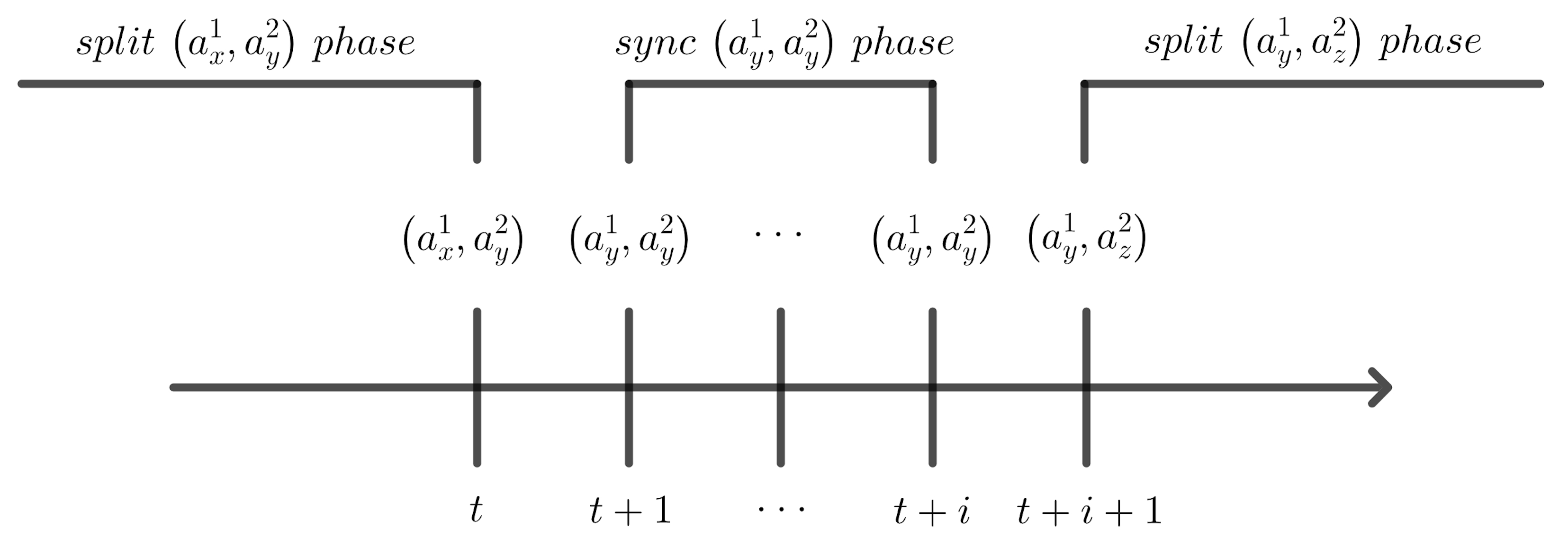
Figure 1: Sync-Split Phase in Diagonal Payoff Matrix Games

Abernethy’s research reveals that during FP iterations, the strategy profiles chosen by players tend to exhibit a regular pattern and often repeat across multiple iterations. Understanding and harnessing this repetitive nature of strategy profiles in FP can be pivotal in accelerating the convergence process. By effectively predicting and calculating the repetition frequency of these strategy profiles, the overall convergence rate of the FP method can be significantly improved.

2.3.3 Pure CFR

PCFR adopts a simple yet effective method by utilizing BR strategies, in contrast to the typical regret matching strategies for next strategy selection. The convergence of PCFR is easy to prove. Firstly, FP’s convergence to NE categorizes it as a regret minimizer (Abernethy et al., 2011). It also means FP satisfied Blackwell approachability (Blackwell, 1956). The CFR framework clarifies that if an algorithm is Blackwell approachable, its regret values will converge to zero (Zinkevich et al., 2007).

Algorithm 3 PCFR

1:  Initialization:

2:  Random initialization $\sigma_{t=1}(I)$. Set $\bar{\sigma}_{t=1}^{i}(I)=\boldsymbol{0}$, $W_{t=0}^{i}(I)=0$, $\bar{Q}_{t=0}^{i}(I)=\boldsymbol{0}$ for all $i\in\mathcal{N}$, $I\in\mathcal{I}$.

3:  for $t=1,2,\dots$ do

4:     for $\forall I\in\mathcal{I}$ do

5:        Observe Utility:

6:        $Q^{i}_{t}(I,a)=\pi_{\sigma_{t}}^{-i}(I)u^{i}(I,\sigma_{t}|_{I\rightarrow a})$

7:        $\bar{Q}^{i}_{t}(I)=\frac{t-1}{t}\bar{Q}^{i}_{t-1}(I)+\frac{1}{t}Q^{i}_{t}(I)$

8:        Next Strategy:

9:        $\sigma^{i}_{t+1}(I)={\arg\max}_{a\in\mathcal{A}(I)}\bar{Q}_{t}^{i}(I,a)$

10:        Update Average Strategy:

11:        $\alpha_{t}=\frac{\pi_{\sigma_{t}}^{i}(I)}{W_{t-1}(I)+\pi_{\sigma_{t}}^{i}(I)}$

12:        $\bar{\sigma}_{t}^{i}(I)=(1-\alpha_{t})\bar{\sigma}_{t-1}^{i}(I)+\alpha_{t}\sigma_{t}^{i}(I)$

13:        $W_{t}^{i}(I)=W_{t-1}^{i}(I)+\pi_{\sigma_{t}}^{i}(I)$

14:     end for

15:  end for

Algorithm 3 is termed Pure CFR because each iteration yields a pure strategy. PCFR leads to a significant computational advantage, with each iteration requiring only $\mathscr{O}\left(|\mathcal{A}||\mathcal{I}|^{-\frac{1}{2}}\right)$ in time complexity, compared to CFR’s $\mathscr{O}(|\mathcal{A}||\mathcal{I}|)$.

3 Method

Our approach integrates ideas from the works of Abernethy and Qi. Drawing from Abernethy’s insights, we developed a novel FP implementation named DW-FP. This method significantly enhances the convergence rate of equilibrium in normal-form games. Inspired by Qi’s research, we extended DW-FP to extensive-form games, resulting in the DW-PCFR.

3.1 DW-FP

In FP algorithms, the same strategy profiles often repeat for multiple iterations. For instance, as shown in Table 1, in Rock-Paper-Scissors (RPS) starting with the strategy profile (R,R), the iteration process reveals repeated strategy profiles in iterations 1$-$3, 4$-$8, 9$-$15, $\ldots$ By calculating the number of repetitions (dynamic weights), we can accelerate FP’s convergence.

Table 1: The Process of Solving RPS Using Q-Value Based FP Algorithm

No. DW-FP Iteration	No. FP Iteration	Player 1$\&$2 (with initial strategy profile (R,R))
		$Q_{t}$ (r,p,s)			$t\bar{Q}_{t}$ (r,p,s)			Next BR strategy	$t\bar{\sigma_{t}}$ (r,p,s)
	$1$	$0$	$1$	-$1$	$0$	$1$	-$1$	P	$1,~{}0,~{}0$
$1$	$2$	-$1$	$0$	$1$	-$1$	$1$	$0$	P	$1,~{}1,~{}0$
	$3$	-$1$	$0$	$1$	-$2$	$1$	$1$	P	$1,~{}2,~{}0$
	$4$	-$1$	$0$	$1$	-$3$	$1$	$2$	S	$1,~{}3,~{}0$
	$5$	$1$	-$1$	$0$	-$2$	-$0$	$2$	S	$1,~{}3,~{}1$
$2$	$6$	$1$	-$1$	$0$	-$1$	-$1$	$2$	S	$1,~{}3,~{}2$
	$7$	$1$	-$1$	$0$	$0$	-$2$	$2$	S	$1,~{}3,~{}3$
	$8$	$1$	-$1$	$0$	$1$	-$3$	$2$	S	$1,~{}3,~{}4$
	$9$	$1$	-$1$	$0$	$2$	-$4$	$2$	R	$1,~{}3,~{}5$
	$10$	$0$	$1$	-$1$	$2$	-$3$	$1$	R	$2,~{}3,~{}5$
	$11$	$0$	$1$	-$1$	$2$	-$2$	$0$	R	$3,~{}3,~{}5$
$3$	$12$	$0$	$1$	-$1$	$2$	-$1$	-$1$	R	$4,~{}3,~{}5$
	$13$	$0$	$1$	-$1$	$2$	$0$	-$2$	R	$5,~{}3,~{}5$
	$14$	$0$	$1$	-$1$	$2$	$1$	-$3$	R	$6,~{}3,~{}5$
	$15$	$0$	$1$	-$1$	$2$	$2$	-$4$	R	$7,~{}3,~{}5$
4	$16$	$0$	$1$	-$1$	$2$	$3$	-$5$	P	$8,~{}3,~{}5$

The key to calculating dynamic weights in FP is conceptualizing it as a pursuit problem. This approach is apt because the next strategy in FP is determined by the action with the maximum Q-value. A strategy change occurs at the point where there’s a shift in the maximum of $t\bar{Q}_{t}$. Our task is to determine how many iterations are required for this shift in the maximum Q-value. Since $t\bar{Q}_{t}$ is the integral of $Q_{t}$, if strategy $a^{\prime}$ has a higher Q-value than the current strategy $a$, the difference $Q^{gap}=t\bar{Q}_{t}(a)-t\bar{Q}_{t}(a^{\prime})$ represents the distance for the pursuit. The change rate $S=Q_{t}(a^{\prime})-Q_{t}(a)$ is the speed of pursuit, and the required pursuit time is $w=Q^{gap}/S$ (dynamic weights in DW-FP). It directly leads to the next BR strategy, streamlining the overall process and significantly speeding up convergence. The specific implementation of DW-FP is shown in Algorithm 4.

Algorithm 4 DW-FP(Ours)

1:  Initialization:

2:  Random initialization $\sigma_{t=1}$. Set $\bar{\sigma}_{t=1}^{i}=\boldsymbol{0}$, $\bar{Q}_{t=0}^{i}=\boldsymbol{0}$, $W^{i}_{t=0}=0$ for all $i\in\mathcal{N}$.

3:  for $t=1,2,\dots$ do

4:     Observe Utility:

5:     $Q_{t}^{gap,i}(a)=W_{t-1}\max_{a^{*}\in\mathcal{A}^{i}}\left(\bar{Q}^{i}_{t-1}(a^{*})-\bar{Q}^{i}_{t-1}(a)\right)$

6:     $Q^{i}_{t}(a)=u^{i}(a,\sigma_{t}^{-i})$

7:     $S^{i}(a)=Q^{i}_{t}(a)-u^{i}\left(\sigma\right)$

8:     if $S^{i}(a)>0$ then

9:        $w^{i}_{t}(a)=Q_{t}^{gap,i}(a)/S^{i}(a)$

10:     else

11:        $w^{i}_{t}(a)=\inf$

12:     end if

13:     $w_{t}=\min_{i\in\mathcal{N}}\min_{a\in\mathcal{A}}w^{i}_{t}(a)$

14:     $\alpha_{t}^{i}=\frac{w_{t}}{W_{t-1}+w_{t}}$

15:     $\bar{Q}_{t}^{i}=(1-\alpha_{t}^{i})\bar{Q}^{i}_{t-1}+\alpha_{t}^{i}Q^{i}_{t}$

16:     Next Strategy:

17:     $\sigma^{i}_{t+1}={\arg\max}_{a\in\mathcal{A}^{i}}\bar{Q}^{i}_{t}$

18:     Update Average Strategy:

19:     $\bar{\sigma}_{t}^{i}(I)=(1-\alpha_{t}^{i})\bar{\sigma}_{t-1}^{i}(I)+\alpha_{t}^{i}\sigma_{t}^{i}(I)$

20:     $W_{t}^{i}=W_{t-1}^{i}+w_{t}^{i}$

21:  end for

In contrast to the complex calculations required in Greedy RM, the computation of $w_{t}$ in DW-FP is simpler. It eliminates the need for intricate optimization methods, greatly enhancing the practicality of algorithm implementation. This simplicity is particularly advantageous considering that DW-FP operates with an iteration complexity of only $\mathscr{O}(|\mathcal{A}|)$, a significant improvement over RM’s $\mathscr{O}(|\mathcal{A}|^{2})$. This efficiency highlights DW-FP’s superiority, especially in large-scale applications where computational resources and time are critical factors.

3.2 DW-PCFR

In the CFR algorithm, the strategy used in each iteration is a mixed strategy, precluding the repetition of identical strategy profiles over multiple iterations. In contrast, PCFR in extensive-form games utilizes pure strategies in every iteration, allowing for the repetition of the same strategy profile across multiple iterations. This distinct feature makes it feasible to apply the DW-FP concept to PCFR in extensive-form games, potentially enhancing its efficiency and effectiveness.

Algorithm 5 DW-PCFR(Ours)

1:  Initialization:

2:  Random initialization $\sigma_{t=1}(I)$. Set $\bar{\sigma}_{t=1}^{i}(I)=\boldsymbol{0}$ $\bar{Q}_{t=0}^{i}(I)=\boldsymbol{0}$, $W^{i}_{t=0}(I)=0$ for all $i\in\mathcal{N}$, $I\in\mathcal{I}$.

3:  for $t=1,2,\dots$ do

4:     for $\forall I\in\mathcal{I}$ do

5:        Observe Utility:

6:        $\bar{Q}^{*i}_{t-1}(I)=\max_{a^{*}\in\mathcal{A}(I)}\bar{Q}_{t}^{i}(I,a^{*})$

7:        $Q_{t}^{gap,i}(I,a)=W^{i}_{t-1}(I)\left(\bar{Q}^{*i}_{t-1}(I)-\bar{Q}_{t}^{i}(I,a)\right)$

8:        $Q^{i}_{t}(I,a)=\pi_{\sigma_{t}}^{-i}(I)u^{i}\left(I,\sigma_{t}|_{I\rightarrow a}\right)$

9:        $S^{i}(I,a)=\pi_{\sigma_{t}}^{-i}(I)\left(Q^{i}_{t}(I,\sigma_{t-1}^{i})-Q^{i}_{t}(I,a)\right)$

10:        if $S^{i}(I,a)>0$ and $Q^{i}_{t}(I,a)>0$ then

11:           $w^{i}_{t}(I,a)=Q_{t}^{gap,i}(I,a)/S^{i}(I,a)$

12:        else

13:           $w^{i}_{t}(I,a)=\inf$

14:        end if

15:        $w_{t}=\min_{i\in\mathcal{N}}\min_{I\in\mathcal{I}^{i}}\min_{a\in\mathcal{A}(I)}w^{i}_{t}(I,a)$

16:        $\alpha_{t}^{i}(I)=\frac{\pi_{\sigma_{t}}^{i}(I)w_{t}}{W^{i}_{t-1}(I)+\pi_{\sigma_{t}}^{i}(I)w_{t}}$

17:        $\bar{Q}_{t}^{i}(I)=(1-\alpha_{t}^{i}(I))\bar{Q}^{i}_{t-1}(I)+\alpha_{t}^{i}(I)Q^{i}_{t}(I)$

18:        Next Strategy:

19:        $\sigma^{i}_{t+1}(I)={\arg\max}_{a\in\mathcal{A}^{i}}\bar{Q}^{i}_{t}(I,a)$

20:        Update Average Strategy:

21:        $\bar{\sigma}_{t}^{i}(I)=(1-\alpha_{t})\bar{\sigma}_{t-1}^{i}(I)+\alpha_{t}\sigma_{t}^{i}(I)$

22:        $W^{i}_{t}(I)=W^{i}_{t-1}(I)+\pi_{\sigma_{t}}^{i}(I)w^{i}_{t}$

23:     end for

24:  end for

In DW-PCFR 5, calculating the dynamic weights $w^{i}_{t}$ for each information set adds little to the overall computational complexity. This approach integrating iterations where PCFR’s strategy profiles repeat, without affecting the convergence. A significant advantage of DW-PCFR is its ability to process only $\mathscr{O}\left(|I|^{-\frac{1}{2}}\right)$ information sets per iteration, compared to CFR+ which requires touching all $\mathscr{O}\left(|I|\right)$ information sets. This efficiency makes DW-PCFR suitable for larger-scale games, surpassing the adaptability of CFR+.

3.3 The Convergence Analysis of DW-FP/PCFR

The iterative process of DW-FP/PCFR is identical to that of FP/PCFR, clearly establishing their convergence properties. The lower bound of their convergence rate is the same as FP/PCFR’s, which is $\mathcal{O}\left(T^{-\frac{1}{2}}\right)$. The crux of understanding DW-PCFR’s efficiency lies in determining how many PCFR iterations equate to a single DW-PCFR iteration. However, we lack a theoretical proof for this equivalence. If Abernethy’s results can be generalized to extensive-form games (Abernethy et al., 2021), then DW-FP/PCFR could potentially achieve a more rapid lower bound convergence rate of $\mathcal{O}\left(T^{-1}\right)$, thus significantly exceeding the performance of existing algorithms.

In extensive-form games, DW-PCFR distinguishes itself as a comprehensive full-traversal algorithm, comparable to CFR+, while also embodying the computational ease of Monte Carlo methods, such as MCCFR. Its fusion of pure strategy execution and exhaustive traversal grants DW-PCFR the dual benefits of hastened convergence and controlled computational complexity. In essence, DW-PCFR combines the rapid convergence characteristic of full traversal algorithms with the resource efficiency inherent in Monte Carlo methods.

3.4 Advantages of DW-FP/PCFR over Greedy RM

Greedy RM and DW-FP are both dynamic weight algorithms. We believe that there are two reasons why Greedy RM is difficult to use in extensive-form games.

Firstly, in contrast to Greedy RM, which requires solving intricate optimization problems to calculate dynamic weights, DW-FP’s use of pure strategies considerably simplifies the computation of dynamic weights.

Secondly, To ensure convergence in extensive-form games, uniform dynamic weights across all information sets are necessary (Zhang et al., 2022). Greedy RM faces challenges in optimizing potential functions and must traverse all information sets in a single iteration. We envision two methods for calculating Greedy RM’s dynamic weights in extensive-form games.

Method 1 directly optimizing all information sets together:

$$w_{t}^{i}=\min_{w^{\prime}}\sum_{I\in\mathcal{I}}\Phi\left(\left(1-\alpha^{i}_{t}(I)\right)\bar{R}_{t-1}^{i}(I)+\alpha^{i}_{t}(I)R_{t}^{i}(I)\right)$$ (6)

where $\alpha^{i}_{t}(I)=\frac{w^{\prime}}{W_{t-1}^{i}(I)+w^{\prime}}$. This is obviously unrealistic, even for some very simple games (such as Leduc with 288 information sets). This will make the potential function extremely complex and impossible to optimize.

Method 2 calculates the dynamic weight of each information set separately as Eq 7, and then obtain a final dynamic weight as Eq 8, which is similar to DW-PCFR.

$$w^{i}_{t}(I)=\min_{w^{\prime}}\Phi\left(\left(1-\alpha^{i}_{t}(I)\right)\bar{R}_{t-1}^{i}(I)+\alpha^{i}_{t}(I)R^{i}_{t}(I)\right)$$ (7)

$$w_{t}^{i}=\min_{I\in\mathcal{I}}w^{i}_{t}(I)$$ (8)

This method will traverse all $\mathscr{O}({|\mathcal{I}|})$ information sets per iteration. In contrast, DW-PCFR only touched $\mathscr{O}\left(|\mathcal{I}|^{-\frac{1}{2}}\right)$ information sets per iteration. As a result, an iteration of DW-PCFR in practical applications is significantly simpler than one of Greedy RM.

4 Experimental Results

Figure 2: The figure illustrates the performance of various algorithms on 30 randomly generated two-player zero-sum games, with matrix payoff entries drawn from a standard normal Gaussian distribution $N(0,1)$. Both axes of the plots are on a logarithmic scale, where the time coordinate is expressed in milliseconds. The shaded regions around each line represent the 95% confidence interval. This setting will also be used in subsequent experiments.

Figure 3: The figure illustrates the performance of various algorithms on extensive-form two-player zero-sum games. The top row of the experiment’s horizontal axis represents the number of iterations, while the bottom row indicates the training time in milliseconds..

4.1 Game Description and Experimental Settings

Our experiments involved matrix games, variants of Kuhn poker (X card Y Pot Kuhn poker) (Kuhn, 1950) and Leduc poker (X card Y Pot Leduc Poker)  (Shi & Littman, 2001), which are widely used for convergence rate testing.

For our analysis in normal-form games, we utilized algorithms such as FP, RM, RM+, and Greedy RM to compare with the proposed DW-FP. In extensive-form games, our comparisons included PCFR, CFR, and CFR+ to compare with the proposed DW-PCFR. Each algorithm was evaluated across 30 runs to ensure statistical reliability, using a single CPU core to standardize the computing environment. Notably, Greedy RM and CFR+ have been recognized as particularly powerful in their respective game categories. The selection of experiment parameters was guided by established best practices (Brown, 2020; Zhang et al., 2022). For more experimental results, please see Appendix A.

4.2 Two-Player Zero-Sum Normal-Form Games

In the experiment of two-player zero-sum random matrix games, the computational complexity of FP algorithms per iteration is $\mathscr{O}(|\mathcal{A}|)$. Conversely, RM algorithms exhibit a higher complexity of $\mathscr{O}(|\mathcal{A}|^{2})$. As a result, relying solely on iteration number as the metric for assessing FP algorithms does not offer an equitable evaluation framework. Therefore, we chose to evaluate our algorithms based on both the number of iterations and the computational time, aiming to ensure a comprehensive and fair comparison.

Figure 2 shows that DW-FP has the fastest convergence rate, surpassing RM+ significantly in both iteration counts and time efficiency. RM+, together with CFR+ in extensive-form games, is recognized for its enhanced convergence rate and plug-and-play capability, frequently considered among the most effective strategies in game theory learning. Nonetheless, DW-FP not only converges more rapidly than RM+ but is also simpler to implement, making it a more advantageous method. Furthermore, DW-FP achieves a convergence rate that is more than an order of magnitude faster than that of Greedy RM. Given that the convergence rates of Greedy RM and DW-FP appear similar when assessed by the number of iterations, this implies that a single DW-FP iteration requires only one-tenth the time of a Greedy RM iteration. This effectively highlights DW-FP’s advantages for engineering implementations.

4.3 Two-Player Zero-Sum Extensive-Form Games

As shown in Figure 3, within the environments of Kuhn Poker (55 nodes and 12 information sets) and Leduc Poker (1945 nodes and 288 information sets), DW-PCFR swiftly surpasses alternative algorithms, consistently achieving a convergence rate of $\mathcal{O}(T^{-1})$.

In the case of 3 Card 5 Pots Leduc Poker, which encompasses 49,384 nodes and 6,399 information sets, DW-PCFR initially demonstrated a slower convergence rate compared to CFR+. Yet, as time progressed, its convergence rate improved, approaching $\mathcal{O}(T^{-1})$. Furthermore, allowing it to achieve faster convergence when evaluated in terms of time.

4.4 The Convergence Rate of DW-FP/PCFR

If Karlin’s conjecture is valid (for which there are currently no known counterexamples), the convergence rate of FP would be $\mathcal{O}\left(T^{-\frac{1}{2}}\right)$. Given that DW-FP/PCFR and Vanilla FP/PCFR are fundamentally the same in nature, the primary distinction lies in the fact that DW-FP/PCFR omits several computational steps through the use of dynamic weights. This raises a crucial question: How many Vanilla FP/PCFR iterations are equivalent to a single iteration of DW-FP/PCFR?

Figure 4: The figure depicts the correlation between the number of iterations for DW-FP and FP

Figure 5: The figure depicts the correlation between the number of iterations for DW-PCFR and PCFR

As illustrated in Figure 4, 5, our analysis indicates that for simpler games, such as the 10-action matrix game and Kuhn Poker, the iteration count for DW-FP/PCFR is roughly the square of the iteration count for Vanilla FP/PCFR. In more complex games, like the 1000-action matrix game and 5 Card Leduc Poker, the correlation between the iterations of DW-FP/PCFR and Vanilla FP/PCFR progressively mirrors a quadratic relationship. Our experimental data showing that as training time increases, DW-FP/PCFR is likely to achieve a convergence rate of $\mathcal{O}(T^{-1})$.

5 Conclusions and Future Work

We introduce two innovative approaches for solving two-player zero-sum games, DW-FP and DW-PCFR. DW-FP is tailored for normal-form games, while DW-PCFR is specifically designed for extensive-form games. Both methods stand out for their use of dynamic weighting, a concept inspired by the Greedy RM algorithm. Yet, they surpass Greedy RM with their simplicity, plug-and-play, faster convergence rates, and tailored suitability for both normal and extensive form games.

Our research confirms that DW-FP and DW-PCFR ensure a convergence rate of $\mathcal{O}\left(T^{-\frac{1}{2}}\right)$. More notably, in the vast majority of cases, these strategies exhibit convergence rates approaching $\mathcal{O}(T^{-1})$, underlining their potent efficacy and efficiency in solving NE.

Our future work will span both theoretical insights and practical applications. On the theoretical front, it is essential to dissect the conditions and underlying reasons that enable the convergence rate to approach $\mathcal{O}(T^{-1})$. Additionally, investigating the connection between our newly introduced DW-FP/PCFR methods and established algorithms such as Follow the Regularized Leader (FTRL)(Shalev-Shwartz & Singer, 2007) and Online Mirror Descent (OMD)(Farina et al., 2021) will be pivotal.

On the practical side, our goal is to integrate sampling with DW-PCFR to expand its capabilities. Although DW-PCFR reduces the number of information sets processed in each iteration, sampling remains indispensable for addressing large-scale problems like Texas Hold’em poker. Our next step involves combining sampling with DW-PCFR to tackle these more extensive challenges effectively.

Appendix A Supplementary Experimental Results

A.1 Kuhn-extension/Leduc-extension poker

We have made improvements to Kuhn and Leduc Poker:

1. The original Leduc and Kuhn poker types are 3 cards, and in the improved game the types are $x\geq 3$ cards;

2. The original Leduc and Kuhn can only raise one fixed chip, but in the improved game it is allowed to raise $y\geq 1$ chips of various sizes. The Bet Action raise size here adopts an equal proportional sequence in multiples of 2. For example, when the blind bet is 1 and $y=4$, the allowed raise action is [1, 2, 4, 8];

A.2 Additional Experimental Results

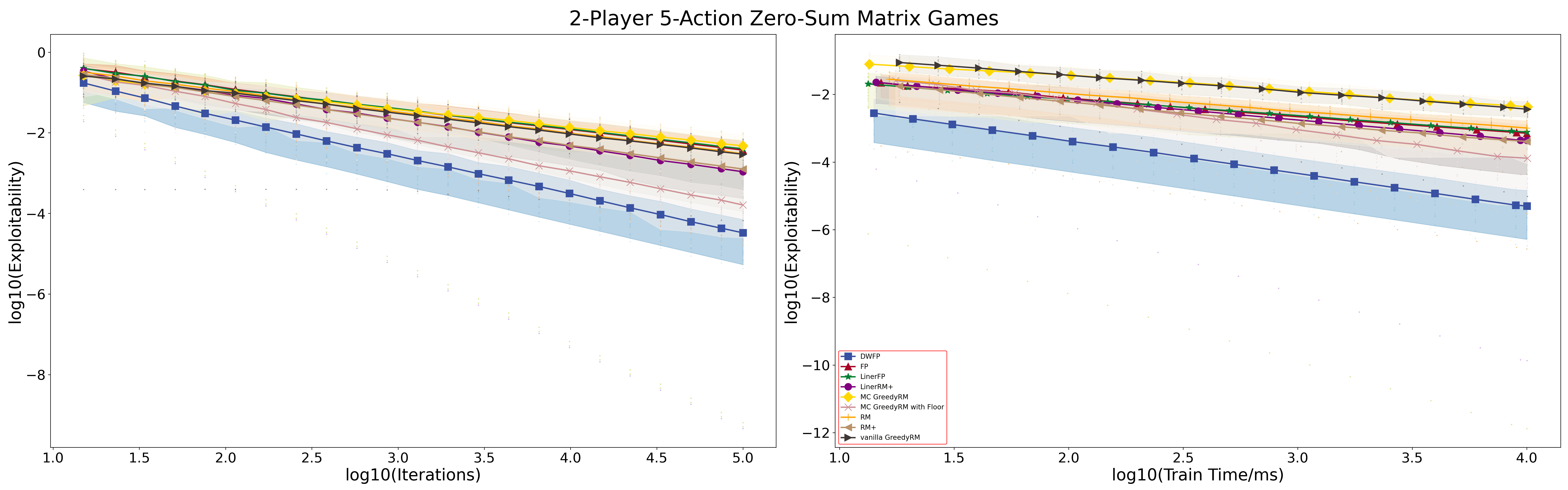
Figure 6:

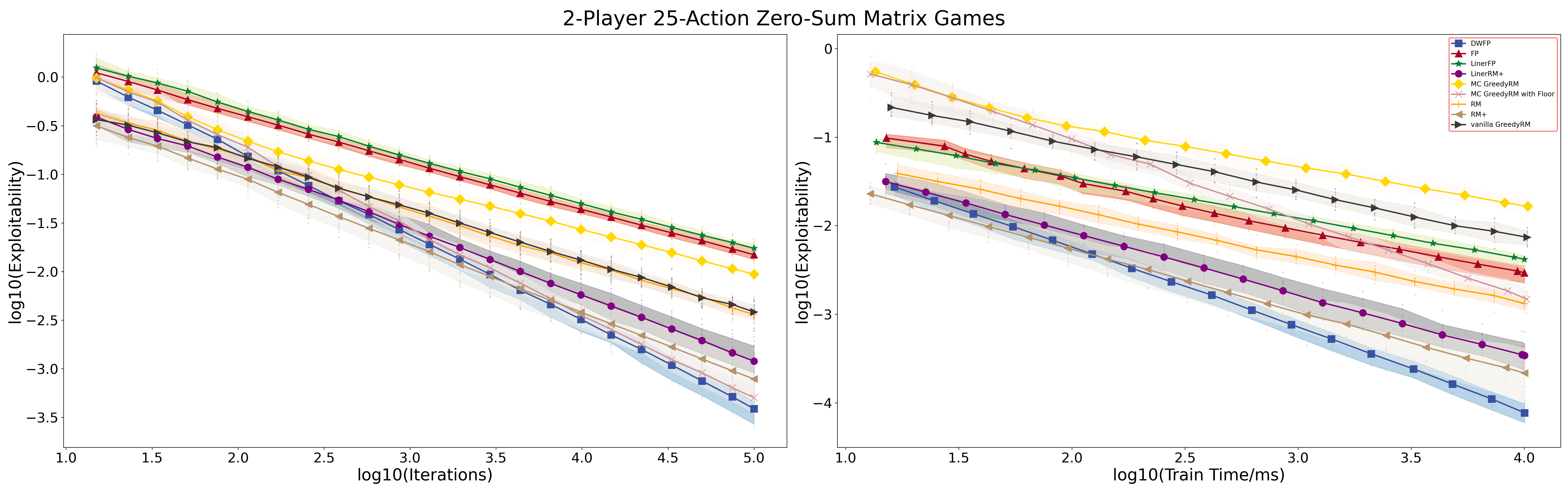
Figure 7:

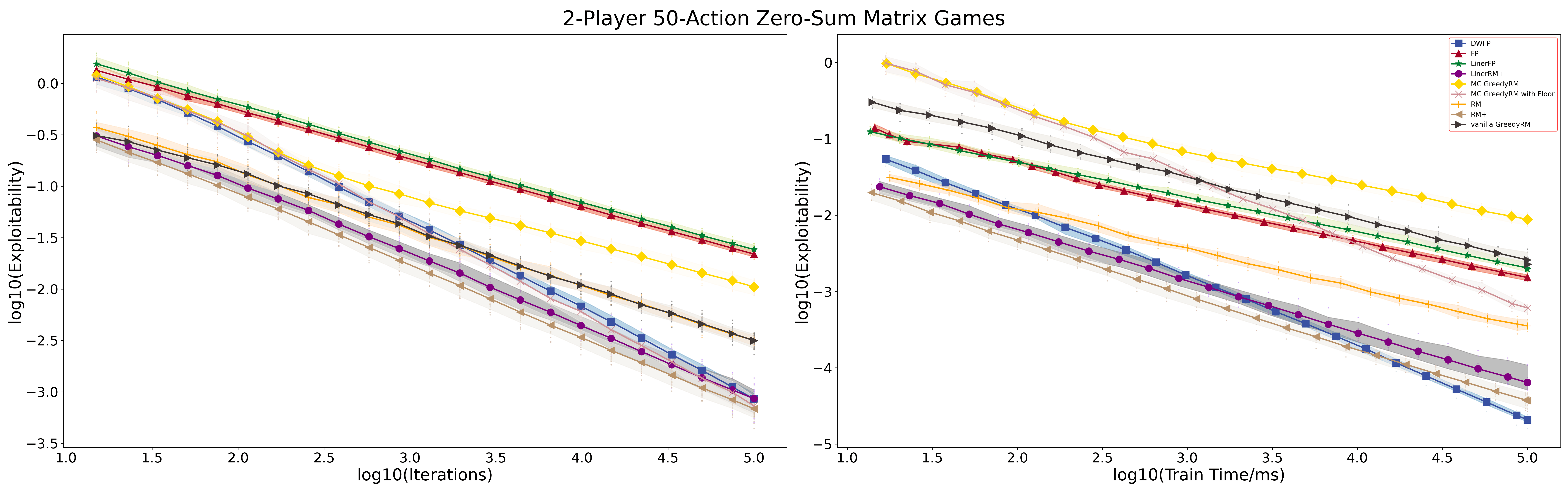
Figure 8:

References

- Abernethy et al. (2011) Abernethy, J., Bartlett, P. L., and Hazan, E. Blackwell approachability and no-regret learning are equivalent. In Proceedings of the 24th Annual Conference on Learning Theory, pp. 27–46. JMLR Workshop and Conference Proceedings, 2011.
- Abernethy et al. (2021) Abernethy, J., Lai, K. A., and Wibisono, A. Fast convergence of fictitious play for diagonal payoff matrices. In Proceedings of the 2021 ACM-SIAM Symposium on Discrete Algorithms (SODA), pp. 1387–1404. SIAM, 2021.
- Blackwell (1956) Blackwell, D. An analog of the minimax theorem for vector payoffs. 1956.
- Blum & Mansour (2007) Blum, A. and Mansour, Y. From external to internal regret. Journal of Machine Learning Research, 8(6), 2007.
- Bowling et al. (2015) Bowling, M., Burch, N., Johanson, M., and Tammelin, O. Heads-up limit hold’em poker is solved. Science, 347(6218):145–149, 2015.
- Brown (1951) Brown, G. W. Iterative solution of games by fictitious play. Act. Anal. Prod Allocation, 13(1):374, 1951.
- Brown (2020) Brown, N. Equilibrium finding for large adversarial imperfect-information games. PhD thesis, 2020.
- Brown & Sandholm (2015) Brown, N. and Sandholm, T. Regret-based pruning in extensive-form games. Advances in neural information processing systems, 28, 2015.
- Brown & Sandholm (2017) Brown, N. and Sandholm, T. Safe and nested subgame solving for imperfect-information games. Advances in neural information processing systems, 30, 2017.
- Brown & Sandholm (2019a) Brown, N. and Sandholm, T. Solving imperfect-information games via discounted regret minimization. In Proceedings of the AAAI Conference on Artificial Intelligence, volume 33, pp. 1829–1836, 2019a.
- Brown & Sandholm (2019b) Brown, N. and Sandholm, T. Superhuman ai for multiplayer poker. Science, 365(6456):885–890, 2019b.
- Cesa-Bianchi & Lugosi (2006) Cesa-Bianchi, N. and Lugosi, G. Prediction, learning, and games. Cambridge university press, 2006.
- Daskalakis & Pan (2014) Daskalakis, C. and Pan, Q. A counter-example to karlin’s strong conjecture for fictitious play. In 2014 IEEE 55th Annual Symposium on Foundations of Computer Science, pp. 11–20. IEEE, 2014.
- Farina et al. (2021) Farina, G., Kroer, C., and Sandholm, T. Faster game solving via predictive blackwell approachability: Connecting regret matching and mirror descent. In Proceedings of the AAAI Conference on Artificial Intelligence, volume 35, pp. 5363–5371, 2021.
- Fudenberg & Levine (1998) Fudenberg, D. and Levine, D. K. The theory of learning in games, volume 2. MIT press, 1998.
- Heinrich et al. (2015) Heinrich, J., Lanctot, M., and Silver, D. Fictitious self-play in extensive-form games. In International conference on machine learning, pp. 805–813. PMLR, 2015.
- Hernandez et al. (2019) Hernandez, D., Denamganaï, K., Gao, Y., York, P., Devlin, S., Samothrakis, S., and Walker, J. A. A generalized framework for self-play training. In 2019 IEEE Conference on Games (CoG), pp. 1–8. IEEE, 2019.
- Karlin (2003) Karlin, S. Mathematical methods and theory in games, programming, and economics, volume 2. Courier Corporation, 2003.
- Kroer & Sandholm (2018) Kroer, C. and Sandholm, T. A unified framework for extensive-form game abstraction with bounds. Advances in Neural Information Processing Systems, 31, 2018.
- Kuhn (1950) Kuhn, H. W. A simplified two-person poker. Contributions to the Theory of Games, 1:97–103, 1950.
- Lanctot et al. (2009) Lanctot, M., Waugh, K., Zinkevich, M., and Bowling, M. Monte carlo sampling for regret minimization in extensive games. Advances in neural information processing systems, 22, 2009.
- Leslie & Collins (2006) Leslie, D. S. and Collins, E. J. Generalised weakened fictitious play. Games and Economic Behavior, 56(2):285–298, 2006.
- Papadimitriou (1994) Papadimitriou, C. H. On the complexity of the parity argument and other inefficient proofs of existence. Journal of Computer and system Sciences, 48(3):498–532, 1994.
- Qi et al. (2023) Qi, J., Feng, T., Hei, F., Fang, Z., and Luo, Y. Pure monte carlo counterfactual regret minimization. arXiv preprint arXiv:2309.03084, 2023.
- Robinson (1951) Robinson, J. An iterative method of solving a game. Annals of mathematics, pp. 296–301, 1951.
- Shalev-Shwartz & Singer (2007) Shalev-Shwartz, S. and Singer, Y. A primal-dual perspective of online learning algorithms. Machine Learning, 69(2-3):115–142, 2007.
- Shi & Littman (2001) Shi, J. and Littman, M. L. Abstraction methods for game theoretic poker. In Computers and Games: Second International Conference, CG 2000 Hamamatsu, Japan, October 26–28, 2000 Revised Papers 2, pp. 333–345. Springer, 2001.
- Tammelin (2014) Tammelin, O. Solving large imperfect information games using cfr+. arXiv preprint arXiv:1407.5042, 2014.
- Vinyals et al. (2019) Vinyals, O., Babuschkin, I., Czarnecki, W. M., Mathieu, M., Dudzik, A., Chung, J., Choi, D. H., Powell, R., Ewalds, T., Georgiev, P., et al. Grandmaster level in starcraft ii using multi-agent reinforcement learning. Nature, 575(7782):350–354, 2019.
- Zhang et al. (2022) Zhang, H., Lerer, A., and Brown, N. Equilibrium finding in normal-form games via greedy regret minimization. In Proceedings of the AAAI Conference on Artificial Intelligence, volume 36, pp. 9484–9492, 2022.
- Zinkevich et al. (2007) Zinkevich, M., Johanson, M., Bowling, M., and Piccione, C. Regret minimization in games with incomplete information. Advances in neural information processing systems, 20, 2007.