Equivariant Hopf bifurcation arising in circular-distributed predator-prey interaction with taxis
Yaqi Chen
Department of Mathematics, Harbin Institute of Technology, Weihai, Shandong 264209, P.R.China.
Xianyi Zeng
Department of Mathematics, Lehigh University, Bethlehem, PA 18015, United States.
Ben Niu
Corresponding author: niu@hit.edu.cnDepartment of Mathematics, Harbin Institute of Technology, Weihai, Shandong 264209, P.R.China.
Abstract
In this paper, we study the Rosenzweig-MacArthur predator-prey model with predator-taxis and time delay defined on a disk. Theoretically, we studied the equivariant Hopf bifurcation around the positive constant steady-state solution. Standing and rotating waves have been investigated through the theory of isotropic subgroups and Lyapunov-Schmidt reduction. The existence conditions, the formula for the periodic direction and the periodic variation of bifurcation periodic solutions are obtained. Numerically, we select appropriate parameters and conduct numerical simulations to illustrate the theoretical results and reveal quite complicated dynamics on the disk. Different types of rotating and standing waves, as well as more complex spatiotemporal patterns with random initial values, are new dynamic phenomena that do not occur in one-dimensional intervals.
Keywords: Predator-prey model, Predator-taxis, Disk, Standing wave, Rotating wave
††preprint:
I Introduction
In order to survive and reproduce, organisms will respond to the surrounding environment, such as staying away from the environment that hinders their own growth and approaching the environment that is conducive to them. This phenomenon of directed movement is called chemotaxis and research on it can be traced back to (Keller and Segel, 1971). In predator-prey models, prey- or predator-taxis can effectively characterize the predator’s directional movement toward habitats with high prey density or the prey’s behavior of perceiving predation risks to avoid predators, respectively. Many studies have focused on the global existence, boundedness, or stability of solutions in models with prey-taxis (Chen, 2023; Choi and Ahn, 2019; He and Zheng, 2015; Jin and Wang, 2017; Giricheva, 2019; Wu et al., 2016) or predator-taxis (Chen and Wu, 2023; Wu et al., 2018; Yoon, 2022). Besides, based on the Hopf bifurcation theory for quasilinear reaction-diffusion systems (Amann, 1991), the existence of center manifolds (Simonett, 1995), and the principle of linearized stability (Drangeid, 1989), there are many studies exploring patterns induced by taxis and bifurcations, through center manifold reduction (Dong and Niu, 2023; Ma et al., 2022; Shi and Song, 2022; Zuo and Song, 2021) or Lyapunov-Schmidt reduction method (Gao et al., 2022; Liu and Guo, 2022; Qiu et al., 2020).
The above studies mostly focus on one-dimensional intervals. Nevertheless, in real life, the interaction between predators and prey frequently occurs in two-dimensional spatial domains. Examples include lakes (Maciej Gliwicz et al., 2006), irregularly shaped protected areas (Khan and Ghaleb, 2003), and circular Petri dishes, which are often chosen as experimental arenas for many studies on the interaction between miniature predators and prey (Banfield-Zanin and Leather, 2016; Meyer et al., 2020). Establishing a predator-prey model on a circular domain can better depict real-world situations. Hence, we consider the Rosenzweig-MacArthur predator-prey model with predator-taxis and time delay on a disk ,
(1)
where represent the density of prey and predator at radius , angle and time , respectively, and . The parameters are all positive and defined in (Shi and Song, 2022), in which the authors investigated the same model on a one-dimensional interval .
With the aid of the phase portraits of the normal form with symmetry (van Gils and Mallet-Paret, 1986), the equivariant bifurcation theory (Guo, 2022; Qu and Guo, 2023), and various wave solutions induced by equivariant bifurcations (Chen et al., 2023a, b), we plan to further explore the joint effect of time delay, predator-taxis and symmetry. Compared to results in (Shi and Song, 2022), spatially inhomogeneous periodic solutions on a disk, including standing and rotating waves are found.
The new wave solutions generated in circular domains have greater practical significance and can offer enhanced insights into characterizing population dynamics within high-dimensional spatial domains. In fact, the disk is a very simple abstraction of a two-dimensional compact simple-connected region, where many methods or ideas can be tested on it before applying to more complicated domains. The research methodologies employed to analyze the properties of these wave solutions in this article can also be further extended to more complex domains.
The rest of the paper is organized as follows. In Section II, we analyze the equivariant Hopf bifurcation around the positive steady state through Lyapunov-Schmidt reduction. In Section III, we simulated spatially inhomogeneous periodic solutions, including standing waves, rotating waves, and more complex periodic spatiotemporal patterns with random initial values.
II Equivariant Hopf bifurcation
In this section, we will study the constant steady states of (1) through a linearization analysis and analyze the equivariant Hopf bifurcation around the steady state through Lyapunov-Schmidt reduction (Liu and Guo, 2022; Guo, 2022; Qu and Guo, 2023; Guo and Wu, 2013). Firstly, we need to introduce some notations in Table 1.
Table 1: Notations
Symbols
Descriptions
the Lebesgue space of integrable functions defined on
the complexification of and
the Banach space of continuous mappings form to with supremum norm
In (Shi and Song, 2022), the authors obtained that the system defined on the interval undergoes spatially inhomogeneous periodic solution at ,
around the unique positive constant steady state , under assumptions -.
.
.
In fact, for , the linearized system of system (1) around is
(2)
where
with .
On a disk, the linearized system (2) restricted to is equivalent to a sequence of functional differential equations (FDEs) on , with a sequence of characteristic equations. Due to the symmetry, some of them have the following form
(3)
and the others are in the following form (Chen et al., 2023a, b)
(4)
with , and the expressions for can be obtained analogously. In this article, we are more concerned about the phenomenon caused by symmetry, so we will study the problem in the case of .
To distinguish the symbols with (Shi and Song, 2022), we record the critical value of the bifurcation parameter as , and
Eq.(4) has a pair of repeated purely imaginary roots , with , under the same assumptions -. Besides, the
transversality conditions hold, i.e. . That is to say, system (1) will generate equivariant Hopf bifurcation at on the disk, by (Shi and Song, 2022; Chen et al., 2023a; Guo and Wu, 2013).
In the following content, we will study the equivariant Hopf bifurcation around and find a periodic solution with a period near . For preparation work,
let
For , note that
.
Then, and are Banach spaces with norms and , respectively. In fact, is a Banach representation of the group , i.e.
For all in , define the inner product as
where is the inner product weighted on .
Normalizing of the period, let and , then system (1) can be transformed into
(5)
where
, for
The above transformation simplifies the study of periodic solutions with time and its similar times of system (1). Finding -periodic solutions of system (1) is equivalent to solving , where is defined by
(6)
Obviously, is -equivariant, i.e. for ,
or
Let be the first derivative of with respect to at . Clearly, the elements of correspond to the -periodic solutions of the linearized equation . Let be the adjoint operator of with that is a kind of bilinear form, defined in (Chen et al., 2023a; Guo and Wu, 2013). Then we have the following results.
Lemma II.1.
Let
For , define
and
Then
is spanned by and is spanned by .
, for , and , for .
Obviously, is a Fredholm operator with index 0 (Gao et al., 2022; Qu and Zhang, 2020), and according to (Guo and Wu, 2013), we can get a space decomposition by -invatiant subspaces of :
where . Next, we aim to obtain the bifurcation mapping corresponding to through Lyapunov-Schmidt reduction. Define two project operators and . Then, and are -equivariant. According to the above space decomposition, can be decomposed into the following two equivalent equations:
where . Due to , and is invertible, by the implicit function theorem, we get a continuously differentiable -equivariant map and satisfies and . Replacing in by , we have
(7)
It is easy to see is -equivariant and satisfies and .
Therefore, by (Guo and Wu, 2013), the periodic solution with time period close to of system (1) corresponds to the solution of (7).
However, finding periodic solutions of system (1) is closely related to the symmetry, which often requires a subspace with simple eigenvalues to study.
Therefore, we can discuss based on the isotropy subgroup theory. By (Qu and Guo, 2023; Guo and Wu, 2013; Golubitsky et al., 1989), the maximal isotropy subgroup of is and .
Obviously, the -symmetric solutions correspond to rotating wave solutions, and satisfy that
(8)
(9)
which correspond to the two possible senses of rotation: clockwise and counterclockwise. Note that with or , and or . It is easy to see that .
Analogously, the -symmetric solutions correspond to a standing wave solutions, and satisfy that
(10)
Note that with , and .
Inspired by (Qu and Guo, 2023; Guo and Wu, 2013), we simplify the problem once again and consider a new restriction mapping or ,
Then, is equivalent to the one-dimensional bifurcation map
(11)
where . Now, our problem is reduced to finding solutions of (11). Clearly, is -equivariant, and satisfies . Therefore, there exist two functions , such that
(12)
Since , then . Let , then is equivalent to either solving or and . Notice that
Therefore,
The implicit function theorem implies that there exists two functions and satisfying , and
(13)
for all sufficient small . Therefore, we have the following equivariant Hopf bifurcation theorem for system (1).
Theorem II.2.
For every maximal isotropy subgroup in which or , is of dimension two, system (1) has a branch of periodic solutions emanating from at , whose spatiotemporal symmetry can be completely characterized by , corresponding to a branch of clockwise (counterclockwise) rotating waves of the form (8) (form (9)) or a branch of standing waves of the form (10).
In what follows, we consider the bifurcation direction and the monotonicity of the period. We use
(14)
to denotes the coefficient of the term in the Taylor expansion of . We still need to compute and , which denote the coefficient of the terms and in the Taylor expansion of , respectively. In fact,
Namely, , thus, the projection operator on them acts as the identity. Following the definition of , we have
By (Guo, 2022; Guo and Wu, 2013; Faria, 2000; Wu, 1996), we summarize the following results.
Theorem II.3.
There exists a branch of -symmetric periodic solutions ( or ), parameterized by , bifurcating from the positive constant steady state of (1). Moreover,
(i) determines the direction of the bifurcation. The bifurcation is supercritical (subcritical), if .
(ii) determines the period of the bifurcation periodic solutions. The period is greater (smaller) than , if .
III Numerical simulations
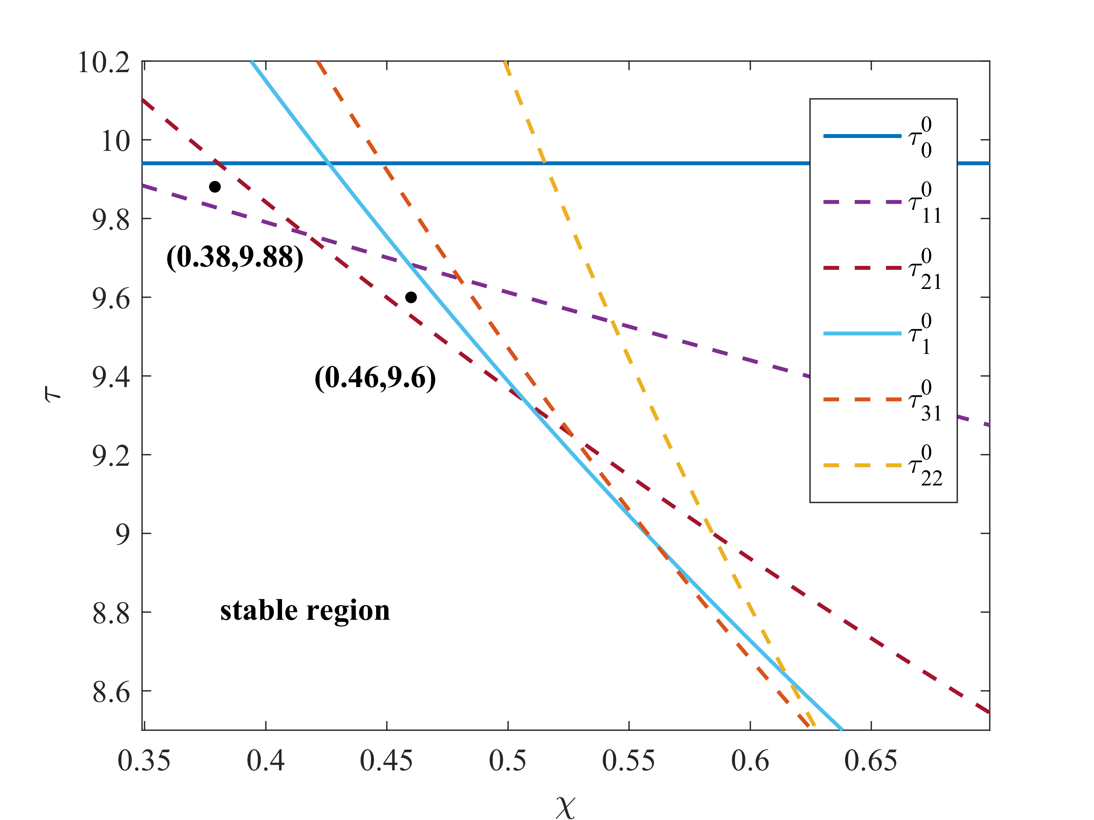
Fixing , at the unique positive constant steady solution , partial bifurcation curves on the plane are shown in Figure 1.
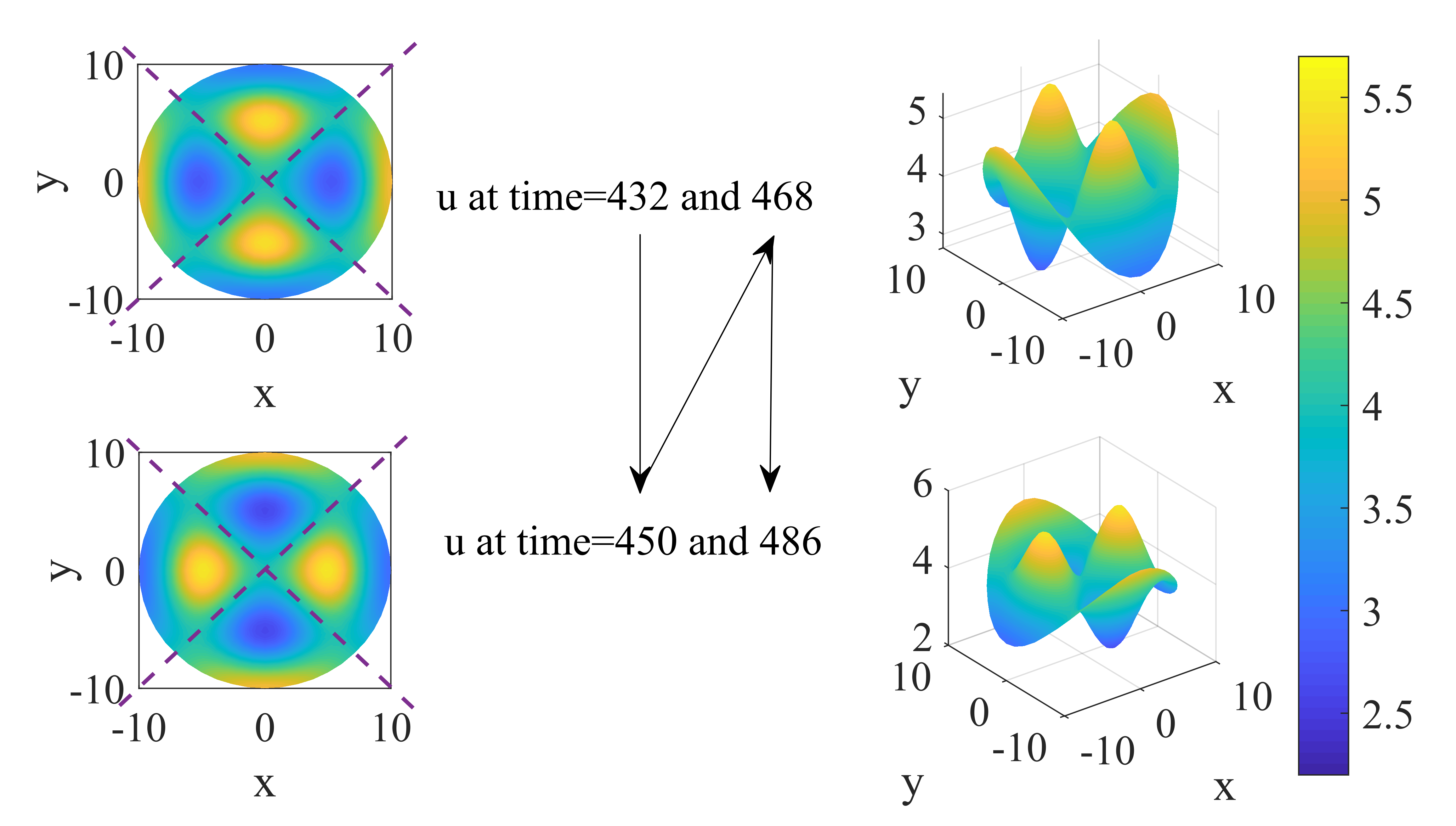
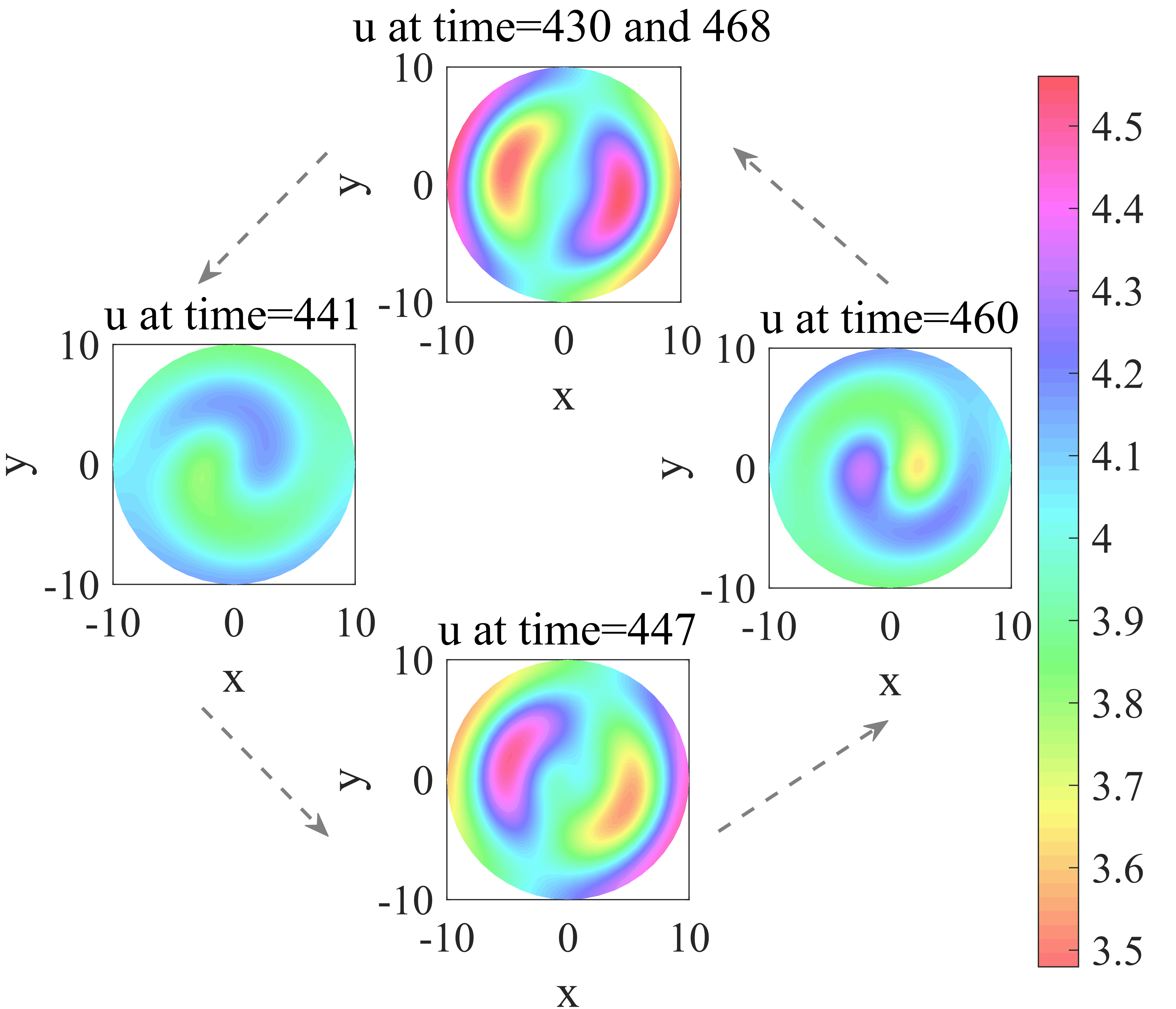
Selecting (Case 1) or (Case 2), the standing wave (see Figure 2 and Figure 3), counterclockwise (see Figure 4) and clockwise rotating wave (see Figure 5) can be found. For simplicity, patterns of the clockwise rotating wave under Case 1 and the counterclockwise rotating wave under Case 2 have not been listed. Besides, more complex periodic spatiotemporal patterns (see Figure 6) with random initial value can be found.
Through numerical calculations, we obtain that under Case 1, , for , and for . Under Case 2, , for , and for .
By Theorem II.3, four bifurcation periodic solutions under two cases are both supercritical the period of them are both greater than .
Figure 1: Partial bifurcation curves on the plane. Parameters are .
(a)
(b)
Figure 2: System (1) generates standing wave that has a fixed axis with .
Initial values are . (a): u; (b): v.
(a)
(b)
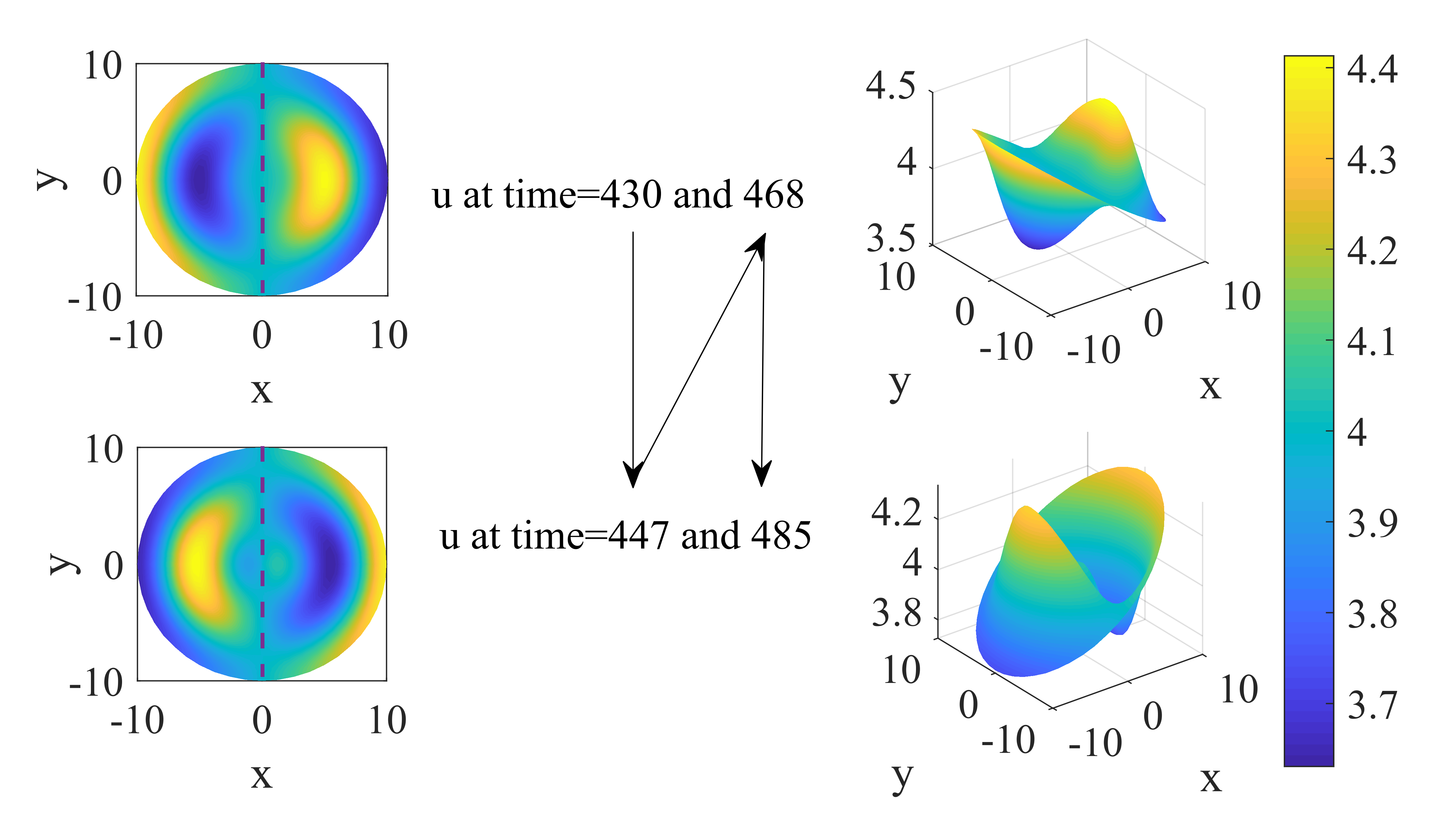
Figure 3: System (1) generates standing wave that has two fixed axes with .
Initial values are . (a): u; (b): v.
(a)
(b)
Figure 4:
System (1) generates counterclockwise rotating wave with . The patterns at four different time within a period are selected to show the periodic changes in population distribution.
Initial values are ,
. (a): u; (b): v.
(a)
(b)
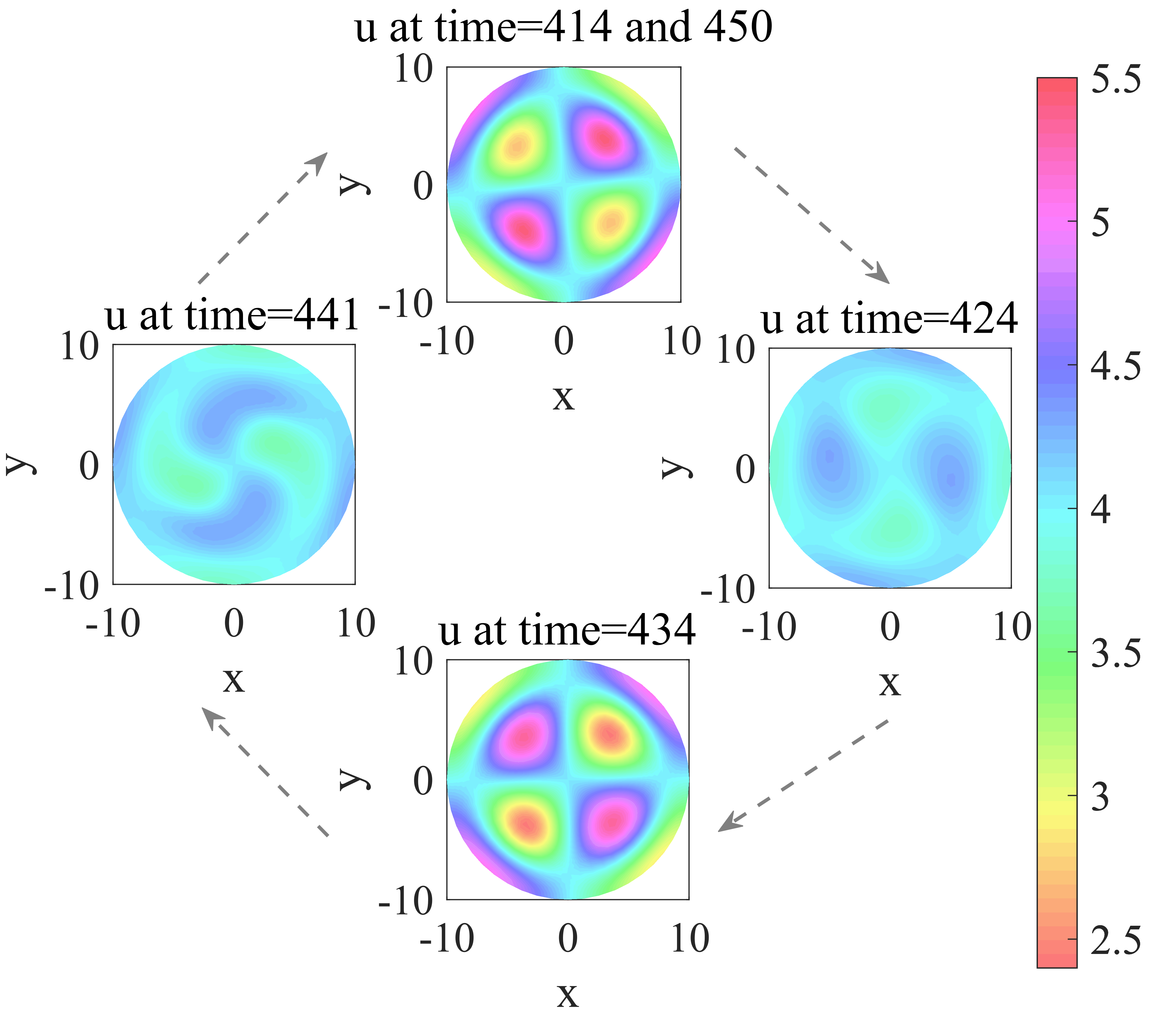
Figure 5:
System (1) generates clockwise rotating wave with . The patterns at four different time within a period are selected to show the periodic changes in population distribution.
Initial values are . (a): u; (b): v.
(a)
(b)
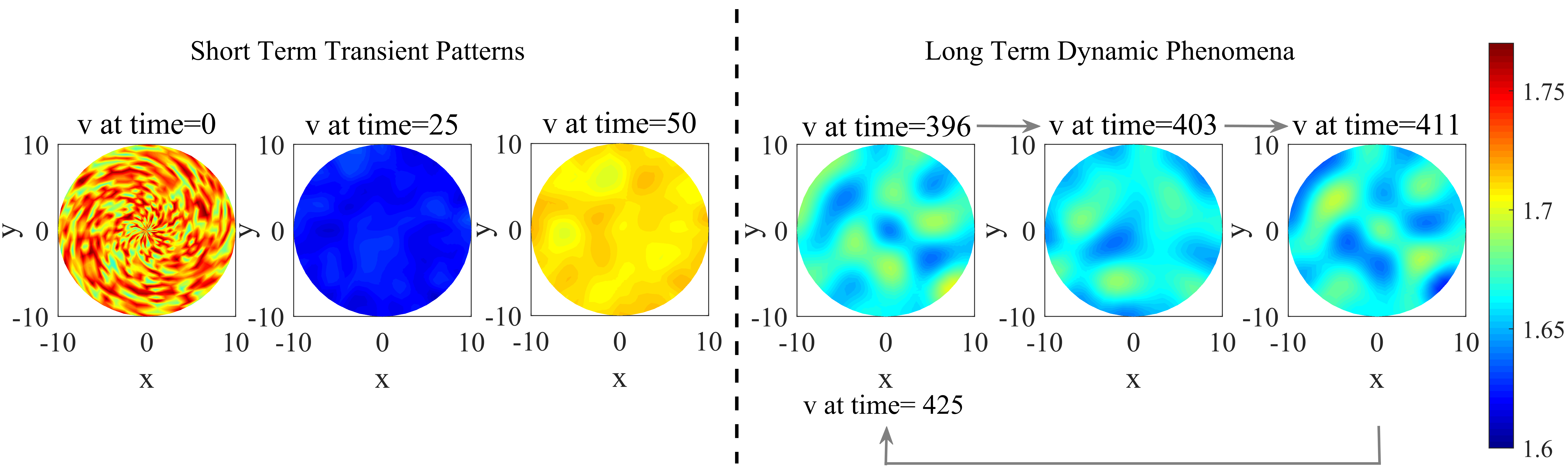
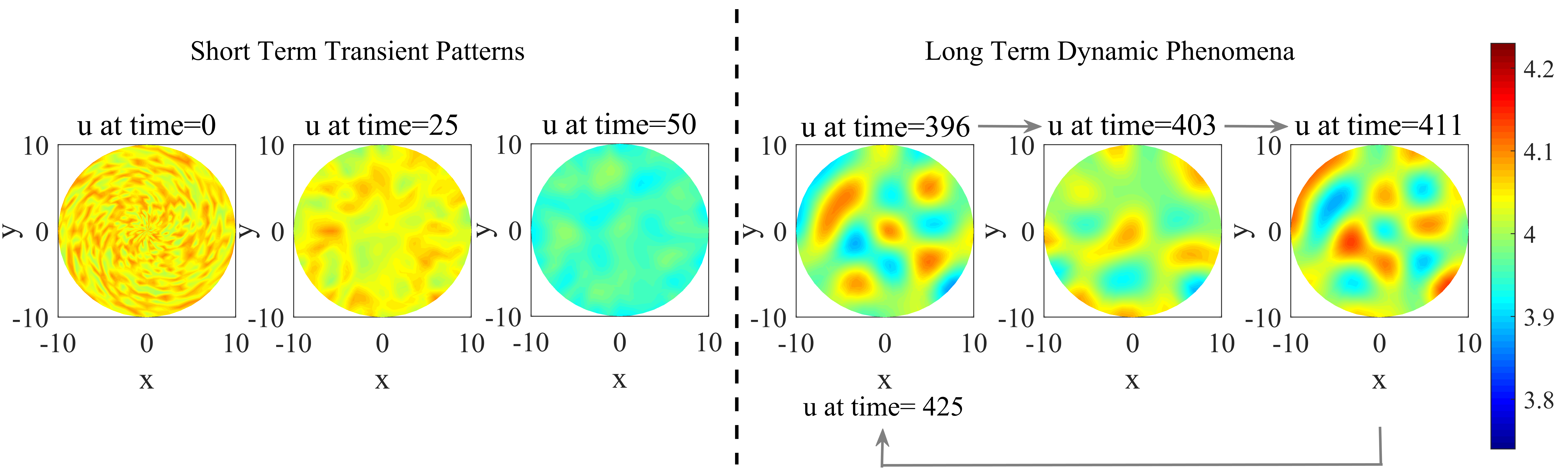
Figure 6: System (1) generates rich transient patterns within a short term and periodic patterns with complex spatial structures after long-term evolution under random initial value and . The patterns at three
different time within a period are selected to show the periodic changes in population distribution.
(a): u; (b): v.
Remark III.1.
On a one-dimensional interval, the solution often quickly converges to a -like spatially inhomogeneous periodic solution (Dong and Niu, 2023; Shi and Song, 2022). However, the two-dimensional domain yields a more significant process of aggregation and dispersion, ultimately presenting periodic patterns with complex spatial structures. The standing wave, rotating wave, and more complex spatiotemporal patterns under different initial conditions on a disk are new interesting phenomena.
IV Conclusion
In this paper, we mainly investigated the equivariant Hopf bifurcation bifurcating from the positive equilibrium
of (1). Methods of Lyapunov-Schmidt reduction and isotropic subgroups were combined to explore the interaction between symmetry, time delay, and taxis on a disk. We have done numerical simulations and spatially inhomogeneous periodic solutions were found, including standing waves, rotating waves, and more complex patterns.
The time delay and taxis can induce the generation of spatially inhomogeneous periodic solutions, while specific forms of standing and rotating waves will be generated on the disk. It is worth mentioning that the algorithm in this paper can also be extended to other fields, such as chemistry, mechanics, nonlinear optics, etc. This extension allows for the exploration of the properties of standing and rotating waves, offering effective control in diverse applications.
Chen et al. (2023a)Y. Chen, X. Zeng, and B. Niu, “Equivariant Hopf bifurcation in a class of
partial functional differential equations on a circular domain,”
(2023a), arXiv:2305.05979 [math.DS] .
Chen et al. (2023b)Y. Chen, X. Zeng, and B. Niu, “Spatiotemporal patterns induced by
Turing-Hopf interaction and symmetry on a disk,” (2023b), arXiv:2309.06133v2 [math.DS] .
Guo and Wu (2013)S. Guo and J. Wu, Bifurcation Theory of Functional
Differential Equations (Springer-Verlag, New York, 2013).
Golubitsky et al. (1989)M. Golubitsky, I. Stewart,
and D. G. Schaeffer, Singularities and Groups in
Bifurcation Theory: Volume II (Springer-Verlag, New York, 1989).
 (b)
(b)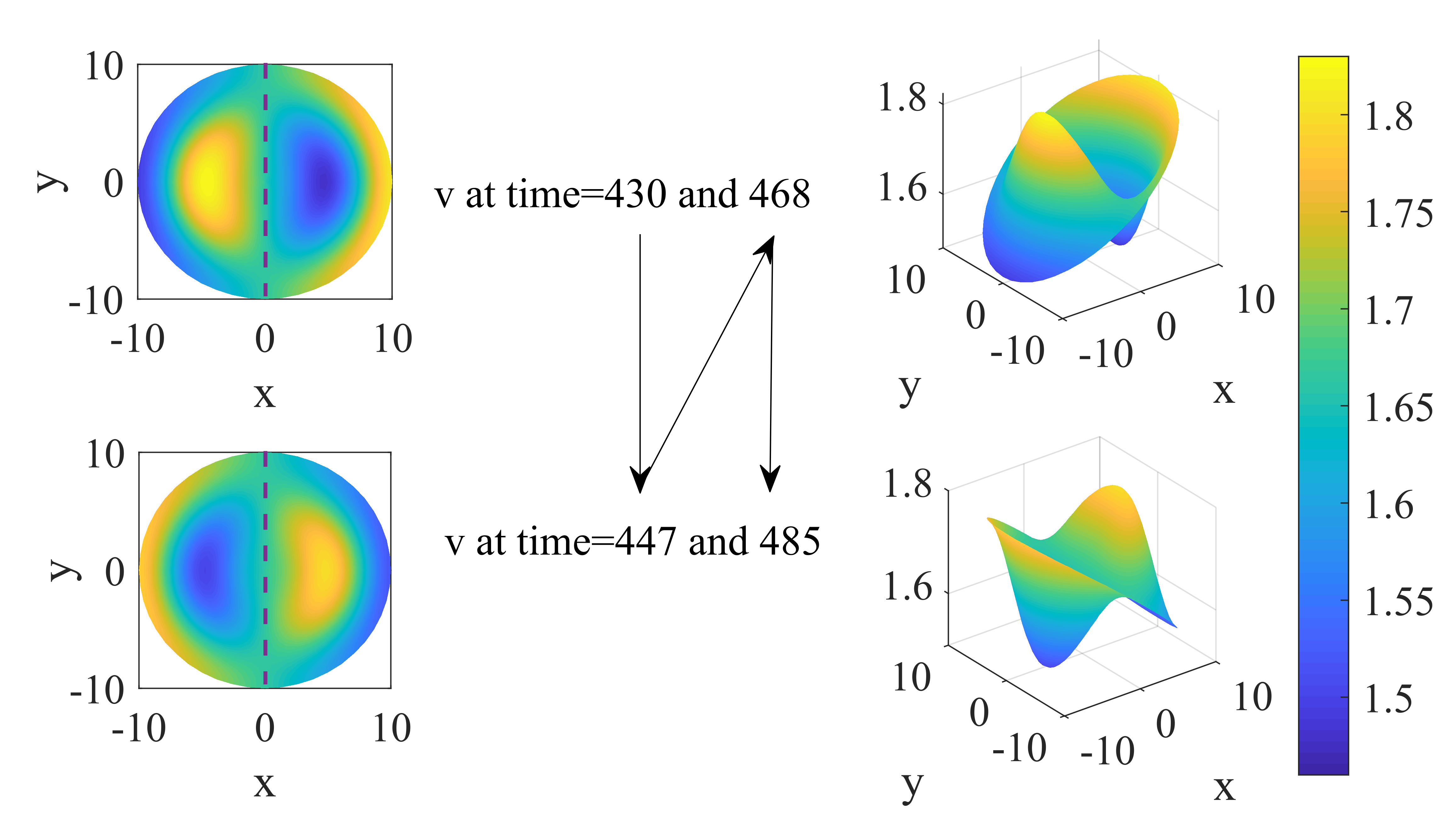
 (b)
(b)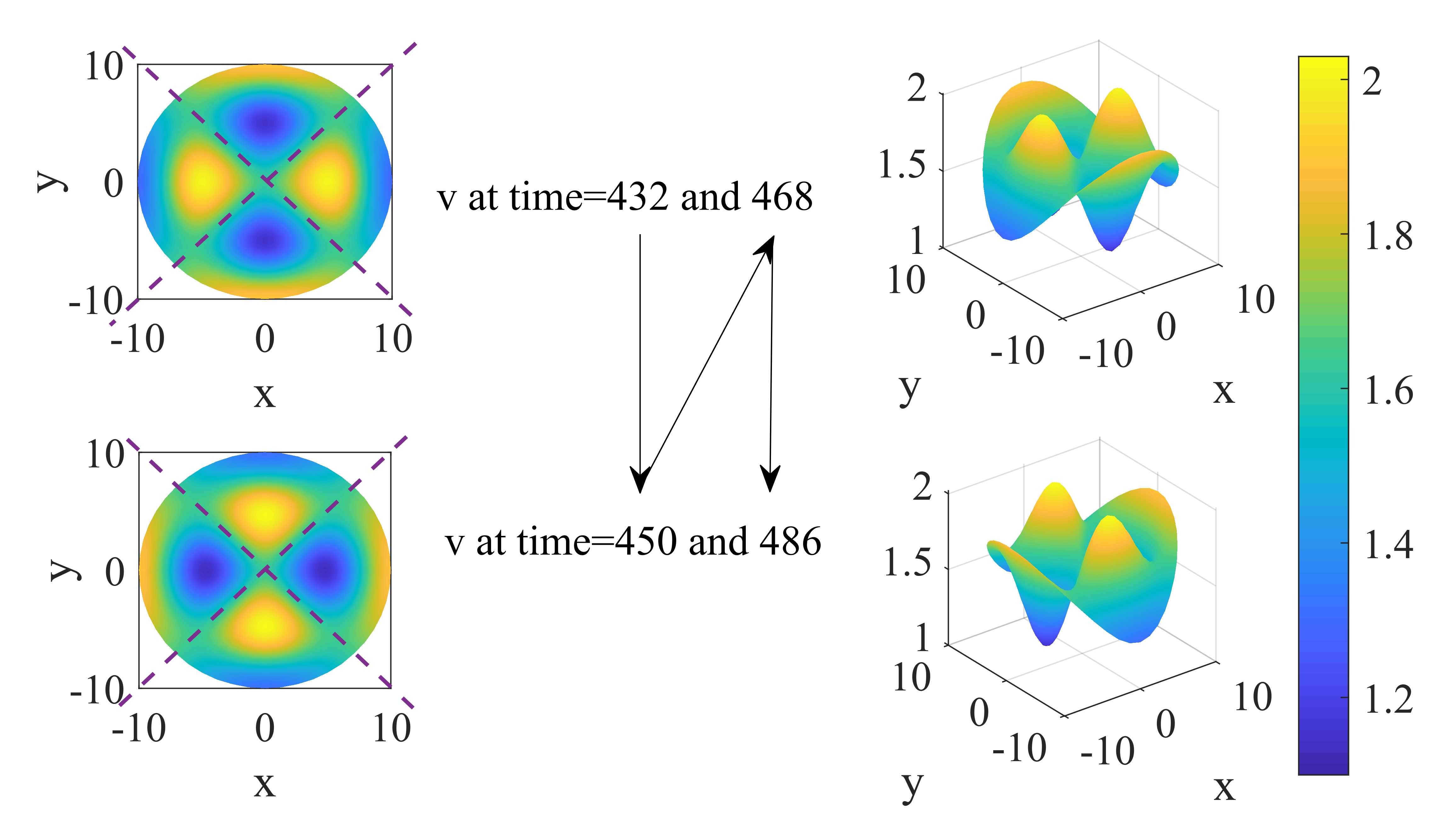
 (b)
(b)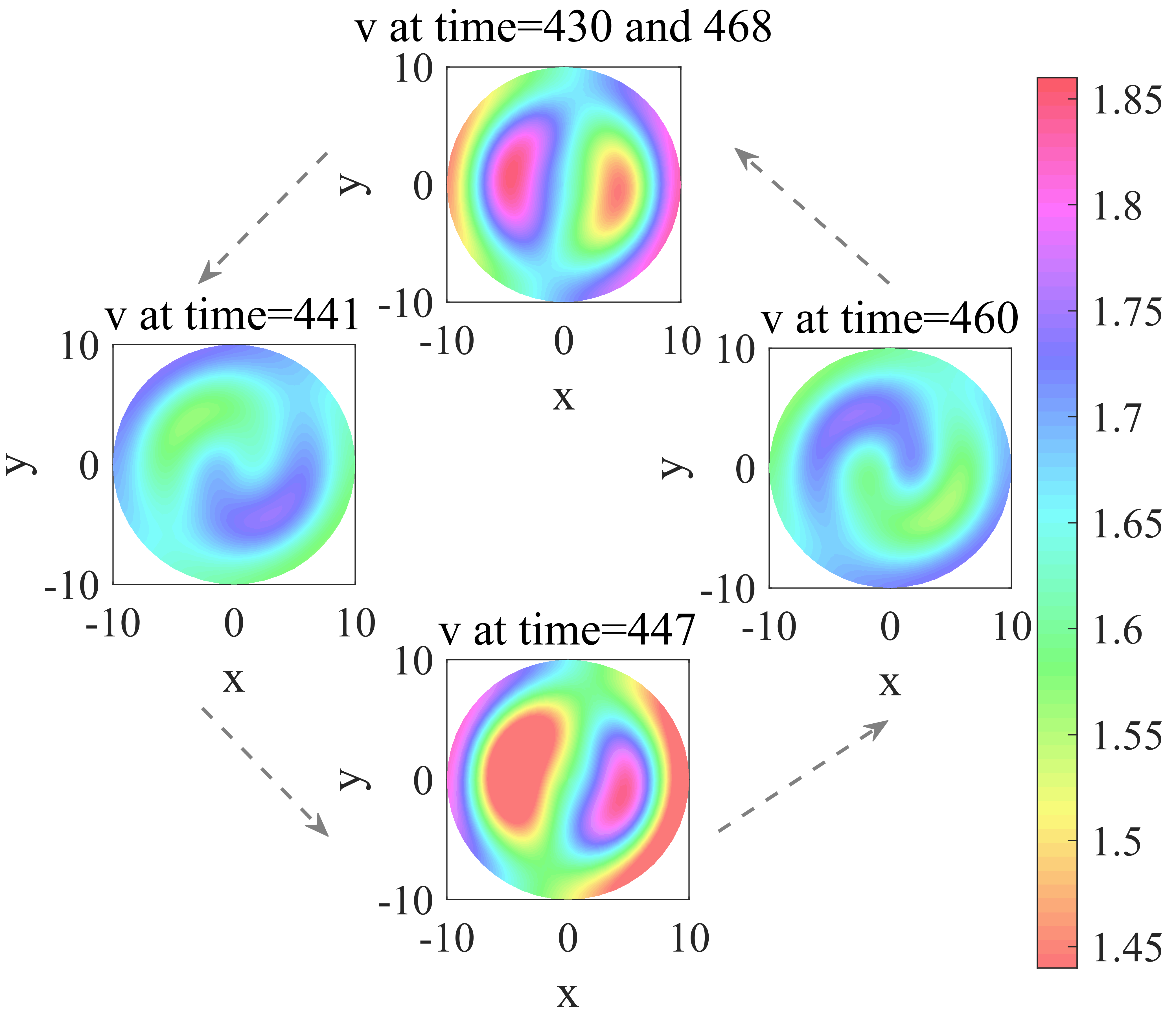
 (b)
(b)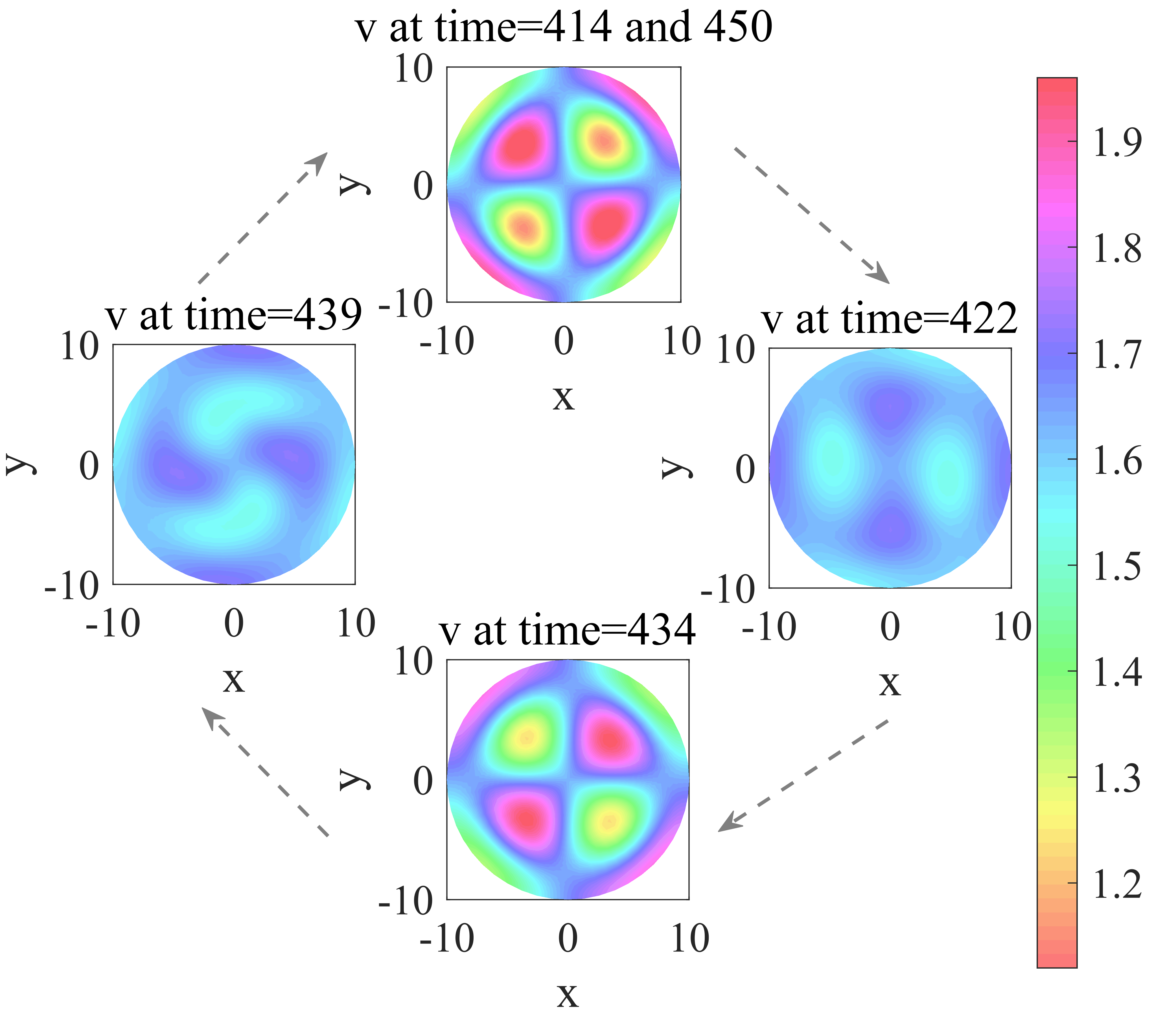
 (b)
(b)