Many-Stage Optimal Stabilized Runge-Kutta Methods for Hyperbolic Partial Differential Equations

Abstract

A novel optimization procedure for the generation of stability polynomials of stabilized explicit Runge-Kutta methods is devised. Intended for semidiscretizations of hyperbolic partial differential equations, the herein developed approach allows the optimization of stability polynomials with more than hundred stages. A potential application of these high degree stability polynomials are problems with locally varying characteristic speeds as found in non-uniformly refined meshes and different wave speeds.

To demonstrate the applicability of the stability polynomials we construct $2N$ storage many-stage Runge-Kutta methods that match their designed second order of accuracy when applied to a range of linear and nonlinear hyperbolic PDEs with smooth solutions. The methods are constructed to reduce the amplification of round off errors which becomes a significant concern for these many-stage methods.

ode short = ODE, long = ordinary differential equation odes short = ODEs, long = ordinary differential equations pde short = PDE, long = partial differential equation pdes short = PDEs, long = partial differential equations ssp short = SSP, long = strong stability preserving tvd short = TVD, long = total varitation diminishing dg short = DG, long = discontinuous Galerkin dgsem short = DGSEM, long = discontinuous Galerkin spectral element method hllc short = HLLC, long = Harten-Lax-Van Leer Contact hll short = HLL, long = Harten-Lax-Van Leer mhd short = MHD, long = magnetohydrodynamics Mhd short = MHD, long = Magnetohydrodynamics glm-mhd short = GLM-MHD, long = generalized Lagrangian multiplier magnetohydrodynamics PERK short = P-ERK, long = Paired-Explicit Runge-Kutta

[1] organization=Applied and Computational Mathematics, RWTH Aachen University,addressline=
Schinkelstrasse 2, city=Aachen, postcode=52062, state=North Rhine-Westphalia, country=Germany. [2] organization=Department of Mathematics and Computer Science, Center for Data and Simulation Science,
University of Cologne,addressline=Weyertal 86-90, city=Cologne, postcode=50931, state=North Rhine-Westphalia, country=Germany.

1 Stabilized Explicit Runge-Kutta Methods

Explicit Runge-Kutta methods are commonly considered the default choice for the integration of hyperbolic pdes. In contrast to implicit methods, explicit methods require only evaluations of the right-hand side instead of solving a potentially nonlinear system of equations. In fact, in the context of hyperbolic pdes typically nonlinear fluxes are of interest. Explicit methods come with the drawback that the maximum stable timestep needs to be significantly reduced which is in the context of (hyperbolic) pdes commonly referred to as the CFL condition [1].

To increase computational efficiency, stabilized explicit Runge-Kutta methods have been introduced already in the 1960s [2, 3, 4] targeting semidiscretizations

$$\boldsymbol{U}(t_{0}) =\boldsymbol{U}_{0}$$ (1.1a)

$$\boldsymbol{U}^{\prime}(t) =\boldsymbol{F}\big{(}\boldsymbol{U}(t)\big{)}$$ (1.1b)

of parabolic pdes. The approach of discretizing the spatial derivatives and leaving time continuous at first is commonly referred to as the Method of Lines approach. Although originally termed for finite difference based spatial discretizations [5] the name persisted and is used nowadays to comprise different discretization techniques like finite elements, finite volumes, and discontinuous Galerkin.

The central idea of stabilized explicit Runge-Kutta methods is to use additional stages primarily to improve the stability properties of the scheme, i.e., allow for larger timesteps. In particular, one usually settles for a moderate order of accuracy and uses the additional degrees of freedom to improve the stability properties of the scheme for a certain spectrum [6, 7, 8]. The fact that the eigenvalues of the Jacobian

$$J(\boldsymbol{U})\coloneqq\frac{\partial\boldsymbol{F}}{\partial\boldsymbol{U}}$$ (1.2)

are for parabolic pdes distributed on the negative real axis enables a successful construction of stabilized explicit Runge-Kutta methods optimized for this special case, see for instance the reviews [9, 10]. The fact that the optimal stability polynomial $P_{S,1}(z)$ of first order accurate methods with $S$ stages is given by the shifted Chebyshev polynomial of first kind $T_{S}(z)$ [2, 3, 11, 12] serves as a valuable guidance to construct higher order approximately optimal stability polynomials [13, 14, 15, 16, 17, 18] which stand on solid ground due to proven existence and uniqueness of optimal stability polynomials with maximum (negative) real axis inclusion [19].

For the purely hyperbolic case, i.e., for eigenvalues $\lambda\in\sigma(J)$ exclusively on the imaginary axis also results for first order accurate methods in terms of Chebyshev polynomials of first kind are known [20, 16, 21, 22]. Approximations to higher order accurate stability polynomials can be found in [23].

For the more general case, i.e., where not only either the real or complex line are of interest, but rather a two-dimensional part of the complex plane, concrete results for stability polynomials are rare. To the best of our knowledge, only for the circle results for first [24] and second [25] order accurate optimal stability polynomials of variable degree $S$ are available. In contrast, one usually has to resort to numerical optimization of the stability polynomials. A nonextensive list includes optimized methods for certain geometrically defined spectra [26, 27], particular equations [28, 29, 30, 31] and spatial discretization techniques [32, 33, 34].

A general framework for maximizing the region of absolute stability of an explicit Runge-Kutta methods for a particular spectrum has been developed in [35] which has been extensively used [36, 33, 37, 38, 39, 40, 41, 42, 32, 43]. The approach presented in [35] is, however, for general spectra limited to polynomials of moderate $(16-20)$ degree due to issues with floating point precision. This is a consequence of the formulating the task to find the maximum admissible timestep as a convex optimization problem in terms of the monomial coefficients of the stability polynomial. The monomial coefficients are also the optimization variables in [26, 29, 30] where polynomials are optimized up to 14, 7, and 8 degrees, respectively.

In this work, we develop a formulation that avoids the inherent ill-conditioning of the monomials-based approach at the cost of turning the optimization problem into a nonlinear one. In particular, instead of parametrizing the polynomial in terms of the monomial coefficients, the stability polynomial $P(z)$ is characterized by the roots of $\big{(}P(z)-1\big{)}/z$. This can be seen as a generalization of the approach employed in [27] wherein the stability polynomial is described by its extrema. While this seems daunting, it will be shown that for a relevant class of spectra an excellent initial guess can be supplied allowing the successful optimization of the highly nonlinear problem. By doing so, we are able to optimize stability polynomials of degrees larger than 100, which to the best of our knowledge is an unprecedented success for general spectra.

A potential application of these high degree stability polynomials are the recently published PERK methods [38, 39, 44] which achieve local time stepping effects by combining a set of stabilized methods. In particular, due to their construction as partitioned Runge-Kutta methods [45] they ensure consistency and conservation which are not trivially satisfied by other classical multirate methods [46]. Being based on the optimization approach developed in [35], the stability polynomials and corresponding PERK methods are currently limited to 16 stages. The availability of higher degree polynomials allows for a potentially even more efficient treatment of e.g. locally refined meshes or varying characteristic speeds. In this work, however, we focus on the optimization of high degree stability polynomials and methods that can be directly constructed thereof. The application to PERK methods is left for future work.

The paper is organized as follows. The motivation for the new optimization approach is presented in Section 2 and Section 3, based on findings for the proven optimal stability polynomials for disk-like spectra. The necessary details required for successful optimization of the problem are discussed in Section 4 which is followed by a discussion of the implementation in Section 5. In Section 6 a couple of high degree optimized stability polynomials are presented. Extensions of the original approach to non-convex spectra are covered in Section 7 and applied in Section 8. The construction of actual Runge-Kutta methods from the high-degree stability polynomials follows in Section 9 with a special focus on internal stability. Section 10 presents the application of the many stage methods to linear and nonlinear problems. Section 11 concludes the paper.

Note on Terminology

For the sake of readability, we will refer to the shifted Chebyshev polynomials of first kind simply as Chebyshev polynomials. As the extreme points of the (shifted) Chebyshev polynomials (of first kind) play a crucial role in this work, we will call them in the interest of brevity simply Chebyshev extreme points. Furthermore, we will refer to the the Chebyshev extreme points with extremal value $+1$ as positive Chebyshev extreme points.

Since a significant part of the paper centers around stability polynomials from which Runge-Kutta methods of certain order may be constructed, we will say that a polynomial of degree $S$ is of order/accuracy $p$ whenever the first $i=0,\dots,p$ coefficients match the first $i=0,\dots,p$ coefficients of the Taylor series of the exponential.

2 Preliminaries

Runge-Kutta methods are single step methods, i.e., when applied to the constant coefficient linear initial value problem (IVP)

$$\boldsymbol{u}(t_{0}=0) =\boldsymbol{u}_{0}$$ (2.1a)

$$\boldsymbol{u}^{\prime}(t) =A\boldsymbol{u}(t)$$ (2.1b)

the new approximation $\boldsymbol{u}_{n+1}$ can be computed from the previous iterate $\boldsymbol{u}_{n}$ as

$$\boldsymbol{u}_{n+1}=R(\Delta tA)\boldsymbol{u}_{n}.$$ (2.2)

Here, $R(z)$ denotes the stability function [6] of the Runge-Kutta method. For implicit methods $R(z)$ is a rational function, while for explicit methods $R(z)$ is a polynomial with real coefficients

$$P_{S}(z;\boldsymbol{\alpha})=\sum_{j=0}^{S}\alpha_{j}z^{j},\quad\boldsymbol{\alpha}\in\mathbb{R}^{S+1}.$$ (2.3)

By comparing 2.2 to the solution $\boldsymbol{u}(t_{n+1})=\exp(A\Delta t)\boldsymbol{u}(t_{n})$ of 2.1b it follows from the definition of the exponential that for a $p^{\prime}$th (linearly) consistent approximation the coefficients $\alpha_{j}$ need to satisfy

$$\alpha_{j}\overset{!}{=}\frac{1}{j!},\quad j=0,\dots,p.$$ (2.4)

It is customary to define the family of polynomials with real coefficients over the complex numbers of degree $S$ and corresponding order of accuracy $p$ as $\mathcal{P}_{S,p}$.

Due to the fact that the stability function $R(z)$ is a polynomial $P(z)$ for explicit methods it follows that the region of absolute stability

$$\mathcal{S}\coloneqq\{z\in\mathbb{C}:|R(z)|\leq 1\}$$ (2.5)

is necessarily bounded. We further define the boundary of the region of absolute stability as

$$\partial\mathcal{S}\coloneqq\{z\in\mathbb{C}:|R(z)|=1\}$$ (2.6)

which will also be called in brief stability boundary.

2.1 Optimization Objective

The optimization objective is now to find the maximum possible timestep $\Delta t_{S,p}^{\star}$ for a polynomial of degree $S$ corresponding to a method with order of accuracy $p$:

$$\underset{P_{S,p}\in\mathcal{P}_{S,p}}{\max}\Delta t\text{ such that }\big{|}P_{S,p}(\Delta t\lambda^{(m)})\big{|}\leq 1,\quad m=1,\dots,M.$$ (2.7)

Here, $\{\lambda^{(m)}\}_{m=1,\dots,M}=\sigma(J)$ are the eigenvalues of the Jacobian 1.2 where the ode system 1.1 corresponds in this work to the semidiscretization of pdes describing typically physical processes. As a consequence, we assume that there are no amplifiying modes among the eigenvalues $\lambda^{(m)}$ corresponding to generation of energy, thus all eigenvalues should have non-positive real part:

$$\text{Re}\big{(}\lambda\big{)}\leq 0\qquad\forall\>\lambda\in\sigma(J).$$ (2.8)

It should be stressed that the maximum possible timestep $\Delta t^{\star}$ is the single optimization target in this work. In particular, we do not focus on the reduction of dispersion or dissipation errors as done for instance in [47, 48, 49] or other objectives like maximum ssp coefficients [50, 51, 33].

2.1.1 Convex Problem Formulation

As noted in [35] 2.7 is for fixed timestep $\Delta t$ a convex optimization problem when parametrizing the stability polynomial $P_{S,p}$ in terms of the monomial coefficients $\boldsymbol{\alpha}$:

$$\underset{\boldsymbol{\alpha}\in\mathbb{R}^{S-p}}{\max}\Delta t\text{ such that }\big{|}P_{S,p}(\Delta t\lambda^{(m)};\boldsymbol{\alpha})\big{|}\leq 1,\quad m=1,\dots,M.$$ (2.9)

Paired with an outer bisection to determine the timestep, 2.9 leads to an efficient optimization routine that can be solved with standard software such as SeDuMi [52] or ECOS [53] for second order cone programs. The downside of formulation 2.9 is that the monomial coefficients scale essentially as $\alpha\sim 1/(j!)$ which limits this approach in standard double precision to about 16 to 20 stages for general spectra. Relieving this inherent issue is the key achievement of our approach motivated in the next subsection.

2.2 Central Observation

The linear consistency requirement 2.4 implies that every at least first order linearly consistent stability polynomial $P_{S,1}(z)$ can be written as

$$P_{S,1}(z;\widetilde{\boldsymbol{r}})=1+z\prod_{j=1}^{S-1}\left(1-\frac{z}{\widetilde{r}_{j}}\right)\\ \eqqcolon 1+z\widetilde{P}_{S-1}(z;\widetilde{\boldsymbol{r}})$$ (2.10)

where the lower degree polynomial $\widetilde{P}_{S-1}$ is parametrized in its complex-conjugated roots $\widetilde{\boldsymbol{r}}\in\mathbb{C}^{S-1}$. Clearly, the roots of the lower-degree polynomial (called from now on pseudo-extrema of the original polynomial) form a subset of the stability boundary $\partial\mathcal{S}$:

$$|P_{S,1}(\widetilde{r}_{j};\widetilde{\boldsymbol{r}})|=|1+\widetilde{r}_{j}\underbrace{\widetilde{P}_{S-1}(\widetilde{r}_{j};\widetilde{\boldsymbol{r}})}_{=0}|=1\quad\Rightarrow\big{\{}\widetilde{r}_{j}\big{\}}_{j=1,\dots,S-1}\subset\partial\mathcal{S}.$$ (2.11)

This observation is particularly useful when the shape of the stability boundary $\partial\mathcal{S}$ can be a-priori roughly estimated. For optimized polynomials of higher degrees, $\partial\mathcal{S}$ will follow the spectrum closely, thus one can use an envelope of the spectrum itself as a reasonable approximation to $\partial\mathcal{S}$. This is discussed in Section 3.2 and Section 7 in more detail.

3 Motivating the Optimization in Pseudo-Extrema

The optimization problem 2.7 for stability polynomials in terms of complex-conjugated pseudo-extrema reads

$$\underset{\widetilde{\boldsymbol{r}}\in\mathbb{C}^{S-1}}{\max}\Delta t\text{ such that }\big{|}P_{S,p}(\Delta t\lambda^{(m)};\widetilde{\boldsymbol{r}})\big{|}\leq 1,\quad m=1,\dots,M.$$ (3.1)

This is a highly nonlinear optimization problem for which we need an excellent initial guess in order to have a reasonable chance to reach the global optimum. In the next section, we will thoroughly motivate a suitable assumption on the distribution of the pseudo-extrema based on results of proven optimal stability polynomials.

3.1 Pseudo-Extrema of Proven Optimal Stability Polynomials for Disks

We direct our attention to examining the pseudo-extrema of known optimal stability polynomials $P_{S,p}(z)$ for circular spectra. For the sake of completeness, the case for parabolic spectra, i.e., eigenvalues on the negative real line, is provided in A.

3.1.1 First Order Consistent Stability Polynomial

As shown in [24], the optimal first order stability polynomial with largest disk inclusion is given by a sequence of Forward Euler steps:

$$P^{\text{Disk}}_{S,1}(z)=\bigg{(}1+\frac{z}{S}\bigg{)}^{S}.$$ (3.2)

For this stability polynomial it holds that the disk with radius $S$

$$D_{S}\coloneqq\{z\in\mathbb{C}:|z+S|\leq S\}$$ (3.3)

is contained in the region of absolute stability $\mathcal{S}$. Consider the positive Chebyshev extreme points $x_{j}\in\mathbb{R}:T_{S}(x_{j})=1$ of the $S$ degree polynomial on the here relevant $[-2S,0]$ interval which are given by

$$x_{j}=S\left(\cos\left(\frac{2j\pi}{S}\right)-1\right),\quad j=0,\dots,\begin{cases}S/2&S\text{ even }\\ (S-1)/2&S\text{ odd }\end{cases}.$$ (3.4)

We give two motivations for considering the Chebyshev extreme points in connection with the pseudo-extrema. First, as outlined in A the pseudo-extrema of (shifted) Chebyshev polynomials are trivially given by the (shifted) positive Chebyshev extreme points. This is of significance since the first order optimal stability polynomial for parabolic spectra is precisely given by the shifted Chebyshev polynomial of first kind. Second, we recall that the Chebyshev extreme points $x_{j}$ can be perceived as the real part of the set of points $z_{j}$ which partition the circle into segments with equal arc length [54]. In that case, the imaginary part $y_{j}$ of $z_{j}$ can be computed as

$$y_{j}=\pm\sqrt{S^{2}-(x_{j}+S)^{2}}=\pm S\sqrt{1-\cos^{2}\left(\frac{2j\pi}{S}\right)}=\pm S\sin\left(\frac{2j\pi}{S}\right),$$ (3.5)

since $\sin\left(\frac{2j\pi}{S}\right)\geq 0,j=0,\dots,S/2$. Consequently, the points $z_{j}=x_{j}\pm iy_{j}$ with $x_{j},y_{j}$ defined as above lie on the stability boundary $\partial\mathcal{S}$ and are thus a valid candidate for the pseudo-extrema. In fact, one can readily show that these points are indeed the pseudo-extrema of $P^{\text{Disk}}_{S,1}(z)$, as stated in the following theorem.

Theorem 1

The $S-1$ pseudo-extrema of $P^{\text{Disk}}_{S,1}(z)$ are given by the positive Chebyshev extreme points with $x_{j}\neq 0$ of $T_{S}(1+z/S)$ with projection onto the circle with radius $S$ centered at $(-S,0)$.

Proof 1

We compute

$$P^{\text{Disk}}_{S,1}(\widetilde{r}_{j})=\left(1+\frac{\widetilde{r}_{j}}{S}\right)^{S} =\left(1+\frac{x_{j}\pm iy_{j}}{S}\right)^{S}$$ (3.6)

$$=\left(1+\frac{S\left(\cos\left(\frac{2j\pi}{S}\right)-1\right)\pm iS\sin\left(\frac{2j\pi}{S}\right)}{S}\right)^{S}$$ (3.7)

$$=\left(\cos\left(\frac{2j\pi}{S}\right)\pm i\sin\left(\frac{2j\pi}{S}\right)\right)^{S}$$ (3.8)

$$=\exp(\pm\,i\,2j\,\pi)\overset{j\in\mathbb{N}}{=}1.$$ (3.9)

As a consequence, we have that

$$\widetilde{P}_{S-1}(\widetilde{r}_{j};\widetilde{\boldsymbol{r}})=\frac{P^{\text{Disk}}_{S,1}(\widetilde{\boldsymbol{r}}_{j};\widetilde{\boldsymbol{r}})-1}{\widetilde{r}_{j}}=0\quad j=1,\dots\begin{cases}S/2&S\text{ even }\\ (S-1)/2&S\text{ odd }\end{cases}$$ (3.10)

where we use the fact that $P_{S,1}(0,\widetilde{\boldsymbol{r}})=1$ which excludes $j=0$ from the set of pseudo-extrema.

Remark 1

Note that for even stability polynomials we have one purely real pseudo extremum $\widetilde{r}_{0}=-S$ and $S-2$ complex conjugated pseudo-extrema. For odd stability polynomials, all pseudo-extrema are complex conjugated. This is in accordance with the motivating observation 2.11 where we established that the pseudo-extrema lie on the boundary of the region of absolute stability $\partial\mathcal{S}$. We also note that the complex-conjugated pseudo-extrema of $P^{\text{Disk}}_{S,1}(z)$ correspond to the real pseudo-extrema with root-multiplicity two of the Chebyshev polynomials $T_{S}(1+z/S^{2})$, see A.

3.1.2 Second Order Consistent Stability Polynomial

For disks/circular spectra there is also an explicit formula for the optimal second order accurate polynomial known [25]. The polynomial

$$P^{\text{Disk}}_{S,2}(z)=\frac{S-1}{S}\left(1+\frac{z}{S-1}\right)^{S}+\frac{1}{S}$$ (3.11)

contains the maximum disk $D_{S-1}$ in its region of absolute stability [25]. As a side note, we realize that $P_{S,2}(z)$ is identical to the second order accurate Runge-Kutta Chebyshev method [55, 56] with infinite damping [57]. Furthermore, as mentioned in [57] $P_{S,2}(z)$ can be written as a sequence of forward Euler steps and belongs consequently to the family of tvd/ssp integrators [58, 59] with optimal ssp coefficient [60].

Theorem 2

The $S-1$ pseudo-extrema of $P^{\text{Disk}}_{S,2}$ are given by the positive Chebyshev extreme points $x_{j}\neq 0$ of $T_{S}\big{(}1+z/(S-1)\big{)}$ when projected onto the circle with radius $S-1$ centered at $\big{(}-(S-1),0\big{)}$.

Proof 2

Analogous to proof of Theorem 1.

Remark 2

As for the first order accurate stability polynomial, we have for even $S$ one real pseudo-extremum $\widetilde{r}_{0}=-(S-1)$ and $S-2$ complex conjugated pseudo-extrema and for odd $S$ a set of $(S-1)/2$ exclusively complex conjugated pseudo-extrema.

The significance of these results is that the pseudo-extrema are distributed with exact equal arc length on the hull of the spectrum, and consequently with approximately equal arc length on the stability boundary for a finite number of stages $S$. In fact, in the limit $S\to\infty$ the stability boundaries converge to the circle and thus the pseudo-extrema are asymptotically distributed with exact equal arc length on th stability boundary.

Especially higher degree stability polynomials have enough flexibility to fully adapt the stability boundary to the envelope of the spectrum. This is the case for even and odd polynomial degrees $S$ as well as first and second order accurate polynomials. To illustrate this, we present Fig. 1 where the pseudo-extrema of second order accurate polynomials $P^{\text{Disk}}_{S,2}$ with degrees $S=12$ and $S=13$ are shown.

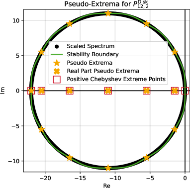
(a) Pseudo-Extrema $\widetilde{r}_{j}$ and boundary of region of absolute stability $\partial\mathcal{S}$ of $P^{\text{Disk}}_{12,2}(z)$ alongside positive Chebyshev extreme points of $T_{12}(1+z/S)$.

(b) Pseudo-Extrema $\widetilde{r}_{j}$ and boundary of region of absolute stability $\partial\mathcal{S}$ of $P^{\text{Disk}}_{13,2}(z)$ alongside positive Chebyshev extreme points of $T_{13}(1+z/S)$.

Figure 1: Optimal second order accurate stability polynomials $P_{S,2}(z)$ given by 3.11 for even LABEL:sub@fig:CircleEven and odd degree LABEL:sub@fig:CircleOdd polynomial. The spectrum corresponds to the canonical first order Finite Volume Upwind/Godunov discretization [61] of the advection equation $u_{t}+u_{x}=0$ on the periodic $[-1,1]$ domain discretized with $500$ cells. In the even degree case LABEL:sub@fig:CircleEven, the lower degree polynomial is odd and thus there is one pure real pseudo extremum at the left end of the spectrum. For odd polynomial degrees LABEL:sub@fig:CircleOdd, the lower degree polynomial is of even degree and we have only complex-conjugated pseudo-extrema. Note also that the segment crossing $0$ is twice the length of the others, which follows from the fact that $P_{S,p}(0)\equiv 1\>\forall\>S,p\geq 1$, cf. 2.10.

3.2 Central Assumption

Based on the findings for the circle we make a central assumption regarding the pseudo-extrema of strictly convex spectra, i.e., where the eigenvalues define a strictly convex set of points in the complex plane. To establish an intuition for this type of spectra we present four exemplarily representatives falling into this category in Fig. 2. We assume that the pseudo-extrema of optimal stability polynomials are distributed with approximately equal arc length on the convex hull of strictly convex spectra.

3.2.1 Strictly Convex Spectra

To motivate this assumption extending the findings for proven optimal spectra of the circle, we display the pseudo-extrema of optimized $P_{16,2}(z)$ polynomials for different spectra in Fig. 2. The optimal stability polynomials and optimal timesteps $\Delta t_{16,2}$ have been computed using the approach developed in [35] and the pseudo-extrema are computed numerically.

We present the spectra of four nonlinear hyperbolic pdes

1. Burgers’ equation

2. 1D Shallow Water equations

3. 1D Ideal Compressible Mhd equations

4. 2D Compressible Euler equations

when discretized with the dgsem [62, 63] using Trixi.jl [64, 65, 66]. We use local polynomials of degrees $1,2,3$ and a range of numerical fluxes and initial conditions, corresponding to both smooth and discontinuous solutions. For the sake of reproducibility we give the precise setups of the semidiscretizations corresponding to the displayed spectra in B.

As seen from Fig. 2 the pseudo-extrema are distributed with approximately equal arc length on the spectrum enclosing curve. Based on this observation we will initialize the pseudo-extrema such that they are distributed with equal arc length on the spectrum enclosing curve, which is assumed to be very close to the optimal stability boundary of higher degree polynomials. The deviations from the equal arc-length initialization are then courtesy of the optimizer.

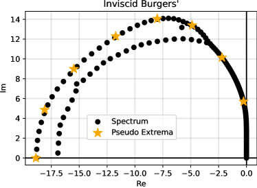
(a) Burgers’ Equation corresponding to the semidiscretization defined by item 1.

(b) 1D Shallow Water Equations corresponding to the semidiscretization defined by item 2.

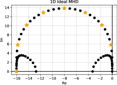
(c) 1D Compressible Ideal MHD corresponding to the semidiscretization defined by item 3.

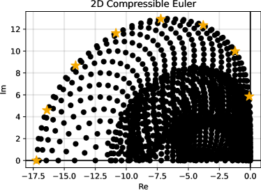
(d) 2D Compressible Euler equations corresponding to the semidiscretization defined by item 4.

Figure 2: Collection of strictly convex spectra of nonlinear hyperbolic pdes and optimized pseudo-extrema $\widetilde{r}_{j}$. The spectra are scaled with the optimal timestep $\Delta t_{16,2}$ in each case.

The significance of the strictly convex spectra stems from the observation that the optimal stability boundary $\partial\mathcal{S}^{\star}$ can be, for a sufficiently high polynomial degree $S$, reasonably well approximated with the convex hull of the eigenvalues. This implies, in turn, that we can use the convex hull of the spectrum as an Ansatz for the initial placement of the pseudo-extrema $\widetilde{\boldsymbol{r}}$. Generalizing the proven results for the circle, the pseudo-extrema are then placed with equal arc length on the convex hull of the spectrum.

4 Detailed Formulation of the Optimization Problem

In this section we discuss the required details to successfully optimize a stability polynomial when parametrized in pseudo-extrema 3.1.

4.1 Constructing Complex-Conjugated Pseudo-Extrema

Since the lower-degree polynomial $\widetilde{P}_{S-1}$ has real coefficients, one has to ensure that the pseudo-extrema $\widetilde{\boldsymbol{r}}$ are complex-conjugated. In principle, this is a difficult task since throughout the optimization it might happen that a previously real pseudo-extremum is moved away from the real axis into the complex plane. Consequently, another real pseudo-extremum has to be set as the corresponding complex-conjugate, effectively changing the number of free optimization variables by introducing an additional constraint. To avoid this switch-like behaviour we set a-priori a number of real and complex-conjugated pseudo-extrema. Based on the previous results, we restrict ourselves for even degree stability polynomials one real and $S-2$ complex conjugated pseudo-extrema and for odd stability polynomials only $S-1$ complex conjugated ones. For strictly convex spectra this is always found to be true, cf. Fig. 2.

4.2 Restriction to Second Quadrant

Due to symmetry around the real axis it suffices to consider either the second or third quadrant in the complex plane only. In this work, we choose the second quadrant, which implies that we consider only complex numbers with non-negative imaginary part. This implies that for real Jacobians 1.2 with complex-conjugated eigenvalues $\lambda_{j}=\overline{\lambda_{j+1}}$ the stability requirement $|P_{S}(\Delta t\lambda^{(m)})|\leq 1$ needs only to be checked for the $m=1,\dots,\widetilde{M}$ eigenvalues with positive imaginary part, thereby also reducing the number of constraints.

4.3 Scaling of the Optimal Timestep

We briefly comment on the scaling of the optimal timestep $\Delta t^{\star}$ with the degree of the stability polynomial $S$. It is well-known that the maximum admissible timestep scales for parabolic spectra covering the real-axis quadratic in $S$ [9, 10]. In contrast, the one-sided imaginary axis inclusion of polynomials with real coefficients is bound by $S-1$ as shown in [67]. In [23] the tighter maximum imaginary stability limit $\sqrt{(S-1)^{2}-1}$ was conjectured and proven for special cases in [68]. The proven optimal stability polynomials for the disk scale both linearly in $S$, see [24, 25]. As a consequence, we consider for general spectra an asymptotically linear scaling

$$\Delta t_{S,p}=\frac{S}{S_{\text{Ref}}}\Delta t_{S_{\text{Ref}},p},$$ (4.1)

which is observed for instance in [35, 38, 34, 32, 41]. It should be mentioned that for $\mathcal{O}(1)$ better than linear scalings are possible, as for these degrees qualitative changes in the shape of the stability boundary still occur. Once the stability boundary is closely adapted to the spectrum, the linear scaling is recovered.

It is immediately clear that once the timestep increases only linearly with more stages $S$ there is no additional efficiency gained. In particular, we observe for the methods with a large number of stages additional complications due to internal stability, see Section 9.1. Nevertheless, many stage stability polynomials are of great value in the context of multirate partitioned Runge-Kutta. As mentioned before, the PERK schemes [38, 39, 44] would benefit from high degree stability polynomials which enable the efficient integration of systems even in the presence of locally restricted CFL numbers.

4.4 Constraints for Higher Order

For higher order $p$-consistent methods $p-1$ equality constraints have to be added to the stability inequality constraints. To obtain second order consistent methods, for instance, the pseudo-extrema have to satisfy

$$\frac{1}{2}\overset{!}{=}-\sum_{j=1}^{S-1}\frac{1}{\widetilde{r}_{j}}$$ (4.2)

which follows from Vieta’s formulas which establish a link between the roots and coefficients of a polynomial. More generally, for a stability polynomial that matches the first $k=0,\dots,p$ coefficients of the exponential $1/(j!)$ we have the additional constraints

$$\frac{1}{k!}\overset{!}{=}(-1)^{k-1}\sum_{\begin{subarray}{c}1=j_{1},j_{2}\dots j_{k-1}\\ j_{1}\neq j_{2}\neq\cdots\neq j_{k-1}\end{subarray}}^{S-1}\frac{1}{\widetilde{\boldsymbol{r}}_{j_{1}}\widetilde{\boldsymbol{r}}_{j_{2}}\dots\widetilde{\boldsymbol{r}}_{j_{k-1}}},\quad k=2,\dots,p.$$ (4.3)

In this work we focus on second order accurate polynomials since for these the linear order constraints (4.3) imply second order convergence also for nonlinear system, without any additional constraints placed on the coefficients of the method [45, 6]. Nevertheless, we also constructed third order accurate stability polynomials for some selected cases.

4.5 Focus on Even Degree Stability Polynomials

From now on we focus on even degree polynomials since they lead to a slightly simpler formulation of the optimization problem. As we are interested in the many stage case, focusing on either even or odd degree case is no severe restriction.

Even degree stability polynomials come with two main advantages. First, we observe for all considered spectra (not only strictly convex) that the left endpoint of the spectrum, in our cases a real eigenvalue, is always selected as one pseudo-extremum, allowing for an even improved initialization. For strictly convex spectra, this is the only real pseudo-extremum, cf. Fig. 1a, Fig. 2, and Fig. 3. The remaining pseudo-extrema can then be initialized with equal arc length starting from the left endpoint of the spectrum.

Second, under the assumption motivated in Section 3.2 and the linear scaling of the timestep one can readily re-use the optimal pseudo-extrema of the $S/2$ degree polynomial as an advanced initialization for the $S$ degree polynomial. In particular, every second pseudo-extremum of the $S$ stability polynomial is essentially known, cf. Fig. 3.

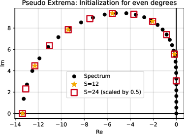
Figure 3: Scaled spectrum $\sigma_{12,2}$ of the 1D linear advection equation $u_{t}+u_{x}=0$ discretized through the dgsem on $[0,1]$ using $16$ cells/elements with DG polynomial degree $3$ and Rusanov/Local Lax-Friedrichs flux. The pseudo-extrema of the $12$ and $24$ degree second order accurate polynomial are computed. To highlight that the relative positions of every second pseudo extremum $\tilde{r}_{2j-1}^{2S}$ agree with $\tilde{r}_{j}^{S}$, the former are scaled by $0.5$ due to the linear scaling of the timestep according to 4.1.

4.6 Construction of the Convex Hull Interpolant

For strictly convex spectra the convex hull defines in the second quadrant actually a strictly concave (strictly convex in the third quadrant) function, which allows to uniquely map the real part of the pseduo-extrema to some corresponding imaginary part. To relax the very steep section near the imaginary axis we add the origin $(0,0)$ to the hull which helps to reduce the slope in that particular segment. This allows to carry out the optimization actually in terms of the real parts of the pseudo-extrema only, cutting the number of optimization variables in half.

Given the (strict) convex hull of the spectrum defined through a set of eigenvalues $\mu^{(j)}\in\sigma^{\text{Hull}}$ and the expected maximum timestep $\Delta t_{S,p}$, we define the scaled spectrum

$$\sigma_{S,p}^{\text{Hull}} \coloneqq\Big{\{}\Delta t_{S,p}\cdot\lambda,\>\lambda\in\sigma^{\text{Hull}}\Big{\}}$$ (4.4)

$$\mu_{S,p}^{(j)} \coloneqq\Delta t_{S,p}\cdot\mu^{(j)}\>.$$ (4.5)

Based on this we construct a piece-wise linear interpolant $I$ as

$$\begin{split}I\left(x;\sigma^{\text{Hull}}_{S,p}\right)\coloneqq\>&\text{Im}\left(\mu_{S,p}^{(j)}\right)+\frac{\text{Im}\left(\mu_{S,p}^{(j+1)}\right)-\text{Im}\left(\mu_{S,p}^{(j)}\right)}{\text{Re}\left(\mu^{(j+1)}_{S,p}\right)-\text{Re}\left(\mu_{S,p}^{(j)}\right)}\left(x-\text{Re}\left(\mu_{S,p}^{(j)}\right)\right),\\ &\text{Re}\left(\mu_{S,p}^{(j)}\right)\leq x<\text{Re}\left(\mu_{S,p}^{(j+1)}\right).\end{split}$$ (4.6)

While quadratic or the classic cubic splines would result in a continuously differentiable interpolant $I$, they lead to numerical artifacts in the very steep sections near the imaginary axis that are a common feature of the dg spectra. For these parts it is observed that linear splines capture the boundary of the stability domain $\partial\mathcal{S}$ best and should be used there. For the less steep regions quadratic and cubic splines were tested, but the increase in approximation quality compared to linear splines was for the majority of cases too small to justify the increased computational costs.

Global interpolation techniques were also tested but familiar problems like Runge’s phenomenon and large over/undershoots in the intervals between the eigenvalues are observed for a variety of approaches, including Bernstein polynomials or mapping to Chebyshev points [69].

It should be mentioned that the spectrum close to the imaginary axis becomes arbitrarily steep and thus the interpolation becomes less reliable in this part. This becomes an issue for stability polynomials of degrees $\mathcal{O}(100)$ since then pseudo-extrema are placed in that region. To solve this problem, one can work with a spectrum enclosing curve $\gamma(\tau):\mathbb{R}\to\mathbb{C}$ instead of a spectrum enclosing function $I:\mathbb{R}\to\mathbb{R}$. By identifying the eigenvalues on the hull $\mu^{(j)}\in\sigma^{\text{Hull}}$ with an arc length parameter $0\leq\tau^{(j)}\leq 1$ the imaginary part can be computed as

$$\begin{split}I_{\text{Im}}\left(\tau;\sigma^{\text{Hull}}_{S,p}\right)=\>&\text{Im}\left(\mu_{S,p}^{(j)}\right)+\frac{\text{Im}\left(\mu_{S,p}^{(j+1)}\right)-\text{Im}\left(\mu_{S,p}^{(j)}\right)}{\tau^{(j+1)}_{S,p}-\tau_{S,p}^{(j)}}\left(\tau-\tau_{S,p}^{(j)}\right),\\ &\tau_{S,p}^{(j)}\leq\tau<\tau_{S,p}^{(j+1)}\end{split}$$ (4.7)

which removes the vanishingly small difference in real parts from the denominator. This, however, comes at the expense that we have to do the interpolation 4.7 also for the real part of the pseudo-extrema, thus doubling the computational work load. As discussed in Section 10, methods with more than hundred stages introduce additional complications related to internal stability. Consequently, we tailor the optimization approach around the more robust $S\sim\mathcal{O}(10)$ case and use the real parts of the pseudo-extrema as the optimization variables.

5 Implementation

In this section, we bundle the aforementioned details into the precise formulation of the solved problems.

5.1 Optimization Problems

Equipped with the interpolant $I(x)$ the optimization of lower-degree polynomial can now be efficiently conducted. The optimization problem 2.7 is first conducted in the real parts $x_{j}=\text{Re}(\widetilde{r}_{j})$ only, i.e.,

$$\max\Delta t\text{ over }\boldsymbol{x}\in\left[\underset{m}{\min}\left\{\text{Re}\left(\lambda_{S,p}^{(m)}\right)\right\},0\right]^{N}\text{ such that }$$ (5.1a)

$$\left|1+\left(\Delta t\lambda^{(m)}\right)\widetilde{P}_{S-1}\left(\Delta t\lambda^{(m)};\boldsymbol{x}+iI\Big{(}\boldsymbol{x};\sigma^{\text{Hull}}_{S,p}\Big{)}\right)\right|\leq 1\quad m=1,\dots,\widetilde{M}.$$ (5.1b)

Note that the number of optimization variables $N$ equals for even stability polynomials $1+\frac{S-2}{2}=\frac{S}{2}$ since we expect one real pseudo extremum and $S-2$ complex conjugated ones.

Due to the sensitive dependence of the stability and order constraints on the pseudo-extrema we conduct a second optimization run where we allow for small corrections $y$ in the imaginary parts of the pseudo-extrema:

$$\boldsymbol{y}\in\left[-\varepsilon\>\underset{m}{\max}\left\{\text{Im}\left(\lambda_{S,p}^{(m)}\right)\right\},\varepsilon\>\underset{m}{\max}\left\{\text{Im}\left(\lambda_{S,p}^{(m)}\right)\right\}\right]^{N}.$$ (5.2)

Here, $\varepsilon$ is the sole hyperparameter needed in our approach which could for all problems be set to $\mathcal{O}\left(10^{-2}\right)$ with default choice $0.02$. The second stage optimization problem reads then

$$\max\Delta t\text{ over }\begin{pmatrix}\boldsymbol{x}\\ \boldsymbol{y}\end{pmatrix}\in\begin{pmatrix}\left[\underset{m}{\min}\left\{\text{Re}\left(\lambda_{S,p}^{(m)}\right)\right\},0\right]^{N}\\ \left[-\varepsilon\>\underset{m}{\max}\left\{\text{Im}\left(\lambda_{S,p}^{(m)}\right)\right\},\varepsilon\>\underset{m}{\max}\left\{\text{Im}\left(\lambda_{S,p}^{(m)}\right)\right\}\right]^{N}\end{pmatrix}$$ (5.3a)

such that

$$\left|1+\left(\Delta t\lambda^{(m)}\right)\widetilde{P}_{S-1}\left(\Delta t\lambda^{(m)};\boldsymbol{x}+i\left[I\Big{(}\boldsymbol{x};\sigma^{\text{Hull}}_{S,p}\Big{)}+\boldsymbol{y}\right]\right)\right|\leq 1\quad m=1,\dots,\widetilde{M}.$$ (5.3b)

The entire algorithm is given in Algorithm 1. In principle, it is also possible to conduct the optimization in real parts and imaginary corrections 5.3 only, i.e., without solving 5.1 first. In all considered cases, however, optimizing the real parts of the pseudo-extrema first led not only to a more robust, but also overall faster optimization process.

1 Perform Algorithm proposed in [35] to obtain $\Delta t_{S_{\text{Ref}},p}$ for certain $S_{\text{Ref}},p$;

2 $\Delta t_{S,p}\leftarrow\Delta t_{S_{\text{Ref}},p}\frac{S}{S_{\text{Ref}}}$;

3 Scale spectrum with expected timestep: $\sigma^{(S,p)}\coloneqq\{\lambda^{(m)}\cdot\Delta t_{S,p}\}_{m=1,\dots,\widetilde{M}}$;

4 Compute convex hull $\sigma^{\text{Hull}}_{S,p}\leftarrow\gamma_{0}\left(\sigma^{(S,p)}\right)$;

5 Compute Interpolant $I\left(x;\sigma^{\text{Hull}}_{S,p}\right)$;

6 if $S,S/2$ are even and results $\boldsymbol{x}^{(S/2)}$ for the $S/2$ degree polynomial exist then

      7 Set every second entry in $\boldsymbol{x}_{0}^{(S)}$ to $2\boldsymbol{x}^{(S/2)}$ ;

      8 Set remaining entries such that $\left(x_{0,j},I\left(x_{0,j};\sigma^{\text{Hull}}_{S,p}\right)\right),j=2,4,\dots,N$ are equally distributed on $I\left(x;\sigma^{\text{Hull}}_{S,p}\right)$;

      

9else

      10 Compute initial guess $\boldsymbol{x}_{0}$ such that $\left(x_{0,j},I\left(x;\sigma^{\text{Hull}}_{S,p}\right)\right),j=1,\dots,N$ are equally distributed on $I\left(x;\sigma^{\text{Hull}}_{S,p}\right)$;

      

11Initialize timestep with maximum possible value $\Delta t_{0}\leftarrow\Delta t_{S,p}^{\star}$;

12 Find best candidate $\Delta t^{\star},\boldsymbol{x}^{*}$ of optimization problem (5.1);

13 Update initial guess $\Delta t_{0}\leftarrow\Delta t^{\star},\boldsymbol{x}_{0}\leftarrow\boldsymbol{x}^{*},\boldsymbol{y}_{0}=\boldsymbol{0}$ ;

14 $(\boldsymbol{x}^{\star},\boldsymbol{y}^{\star})\leftarrow$ Solve second stage optimization problem (5.3);

15 return $\widetilde{\boldsymbol{r}}\leftarrow\boldsymbol{x}^{\star}\pm i\left[I\left(\boldsymbol{x}^{\star};\sigma^{\mathrm{Hull}}_{S,p}\right)+\boldsymbol{y}^{\star}\right]$;

16 return $\Delta t_{S,p}^{\star}\leftarrow\Delta t^{\star}$;

Algorithm 1 Optimization problem in pseudo-extrema.

5.2 Feasibility Problems

Under assumption that we can indeed realize the optimal timestep $\Delta t_{S,p}$ one can formulate the optimization problems 5.1, 5.3 actually as feasibility problems by fixing $\Delta t=\Delta t_{S,p}$ and search for $\boldsymbol{x},\boldsymbol{y}$ satisfying the stability and order constraints. The feasibility problem corresponding to 5.1 reads then

$$\text{Find }\boldsymbol{x}\in\left[\underset{m}{\min}\left\{\text{Re}\left(\lambda_{S,p}^{(m)}\right)\right\},0\right]^{N}\text{ such that }$$ (5.4a)

$$\left|1+\left(\Delta t_{S,p}\lambda^{(m)}\right)\widetilde{P}_{S-1}\left(\Delta t_{S,p}\lambda^{(m)};\boldsymbol{x}+iI\Big{(}\boldsymbol{x};\sigma^{\text{Hull}}_{S,p}\Big{)}\right)\right|\leq 1\quad m=1,\dots,\widetilde{M}.$$ (5.4b)

and the analogy to 5.3 is given by

$$\text{Find }\begin{pmatrix}\boldsymbol{x}\\ \boldsymbol{y}\end{pmatrix}\in\begin{pmatrix}\left[\underset{m}{\min}\left\{\text{Re}\left(\lambda_{S,p}^{(m)}\right)\right\},0\right]^{N}\\ \left[-\varepsilon\>\underset{m}{\max}\left\{\text{Im}\left(\lambda_{S,p}^{(m)}\right)\right\},\varepsilon\>\underset{m}{\max}\left\{\text{Im}\left(\lambda_{S,p}^{(m)}\right)\right\}\right]^{N}\end{pmatrix}$$ (5.5a)

such that

$$\left|1+\left(\Delta t_{S,p}\lambda^{(m)}\right)\widetilde{P}_{S-1}\left(\Delta t_{S,p}\lambda^{(m)};\boldsymbol{x}+i\left[I\Big{(}\boldsymbol{x};\sigma^{\text{Hull}}_{S,p}\Big{)}+\boldsymbol{y}\right]\right)\right|\leq 1\quad m=1,\dots,\widetilde{M}.$$ (5.5b)

In practice, the feasibility problems are solved significantly faster than their optimization counterparts. Note that no conceptual changes to Algorithm 1 are necessary, as the timestep handling in Lines 1 and 1 can be omitted and 5.4 and 5.5 are solved in Lines 1 and 1, respectively.

5.3 Software

Both optimization and feasibility problem are solved via Ipopt: Interioir Point OPTimizer [70], an optimization software designed for general non-linear problems. The herein used required linear solver is MUMPS: MUltifrontal Massively Parallel sparse direct Solver [71, 72] with optional package METIS [73]. Being a derivative based optimizer, Ipopt requires the Jacobian matrix and Hessian tensor of the constraints (and objective) to construct the Lagrangian of the problem. Here, the derivatives are computed algorithmically via dco/c++ [74] which requires only the adaption of some boilerplate code. Besides being much more computationally efficient than approximating the derivatives using finite differences, algorithmic differentiation provides exact derivatives (up to machine precision). This is especially relevant in this case, since the stability constraints are very sensitive with respect to the pseudo-extrema, i.e., small deviations in $\boldsymbol{x}$ can make the difference between a stable and an unstable method. This was observed when Matlab’s function for general nonlinear optimization, fmincon failed in finding the optimal solution. Therein, finite difference approximations of Jacobians and Hessians are used and consequently, the optimization is much less reliable than Ipopt combined with dco/c++.

In terms of complexity the proposed algorithms scales linearly in the number of constraints (stability constraints at eigenvalues and $p-1$ order constraints) $\widetilde{M}$ and quadratic in the number of unknowns (pseudo-extrema with distinct real part) $N$.

It should be mentioned that Ipopt provides many options which can significantly speed up the optimization/feasible point search. Most notably, one should specify grad_f_constant yes which ensures that the gradient of the objective is only evaluated once and the Hessian not at all. An option for a constant objective function as the case for the feasibility problems is not supported, but can actually be implemented by changing only two lines of the Ipopt source code [75]. Furthermore, for many problems the Hessian of the Lagrangian may be successfully approximated using the Limited-memory BFGS method [76] which is activated by specifying the option hessian_approximation limited-memory, resulting in significant speed up. In terms of tolerances, we demand satisfaction of the constraints to machine precision by setting constr_viol_tol 1e-16.

Furthermore, in most cases it suffices to supply only the convex hull and a small subset of the eigenvalues instead of the entire spectrum. This can be seen from e.g. Fig. 4a and Fig. 4d where the stability constraint at the ”interior” eigenvalues is usually satisfied without being explicitly enforced. One has to ensure, however, that there is always a larger number of constraints than pseudo-extrema to prevent degenerate cases where the roots of the stability polynomial are placed exactly on the eigenvalues, thus allowing in principle infinitely large timesteps.

The source code is made publicly available on GitHub [77].

6 Optimal Stability Polynomials for Strictly Convex Spectra

Here, we present many-stage optimal stability polynomials corresponding to first and second order for the spectra shown in Fig. 2. For each spectrum, we compute $\Delta t_{16,p}$ and $P_{16,p}(z)$ using the approach developed in [35]. Equipped with the optimal timestep, we supply the expected timestep according to 4.1 to the feasibility problems 5.4, 5.5. For every spectrum, we start with a moderate number of stages ($26-32$) and then double the number of stages to utilize the equal arc length property for even spectra discussed in Section 4.5.

The computed pseudo-extrema alongside the constraining list of eigenvalues are provided as supplementary material to this manuscript. Optimal stability polynomials are constructed for:

1. Burgers’ Equation: We find the optimal stability polynomials of first, second, and third order with degrees $32,64,128$ constrained by $\widetilde{M}=129$ eigenvalues. In particular, we make use of the property discussed in Section 4.5 by conducting the optimization sequentially, i.e., first performing the optimization for $S=32$, re-using this results for the initialization of the $S=64$ polynomial and in turn using this results for the final $S=128$ polynomial. The pseudo-extrema and contours of the optimal $P_{64,2}(z)$ stability polynomial are displayed in Fig. 4a.

   To highlight the efficiency of our approach, we provide the Ipopt runtimes for the feasibility problem runs in Table 1. We emphasize that we do not intend to compare the runtimes of Algorithm 1 to the optimization problem from [35] - instead, we would like to stress that equipped with an optimal timestep for a low degree polynomial, we can quickly compute the higher degree optimal ones.

   	$t[s]$
   Stages $S$	$1^{\text{st}}\text{ Order}$	$2^{\text{nd}}\text{ Order}$	$3^{\text{rd}}\text{ Order}$
   16 (Alg. from [35])	15.531	15.346	15.076
   32 (Algorithm 1)	0.478	0.879	1.183
   64 (Algorithm 1)	1.551	2.869	2.276
   128 (Algorithm 1)	9.383	8.845	8.549
   Cumulative $t$	26.942	27.939	27.084

   Table 1: Runtimes of feasibility problems for different degrees constrained to spectrum of Burgers equation. The times are obtained on a Dell Precision 5570 laptop equipped with an Intel i7-12800H.

2. 1D Shallow Water equations: Here we optimize polynomials of degrees $30,60$, and $120$ constrained by $\widetilde{M}=117$ eigenvalues, again in a sequential manner. The pseudo-extrema and contours of the optimal $P_{60,2}(z)$ stability polynomial are displayed in Fig. 4b. The CPU times are very similar to Burgers’ equation with total $30.687s$ for the computation of the first order accurate stability polynomial and $28.726s$ for the second order case.

3. 1D Ideal compressible mhd: Polynomials of degrees $28,56$, and $112$ are found satisfying the $\widetilde{M}=252$ stability constraints due to the eigenvalues. The pseudo-extrema and contours of the optimal $P_{56,2}(z)$ stability polynomial are displayed in Fig. 4c. The generation of the $112$ degree stability polynomial takes $94.433s$ and $98.377s$ for first and second order case, respectively.

4. 2D Compressible Euler equations: To conclude this result section, we generate stability polynomials with degrees $26,52$, and $104$ for a reduced set of $\widetilde{M}=717$ eigenvalue constraints. The pseudo-extrema and contours of the optimal $P_{52,2}(z)$ stability polynomial are displayed in Fig. 4d. Due to the quadratic scaling in the number of constraints we have significantly longer runtimes then in the previous cases, with total $2.456\text{ min}$ for the first order and $8.55\text{ min}$ for the second order case. Note that these runtimes can be significantly reduced if only a small portion of the eigenvalues alongside the convex hull thereof is supplied as constraints.

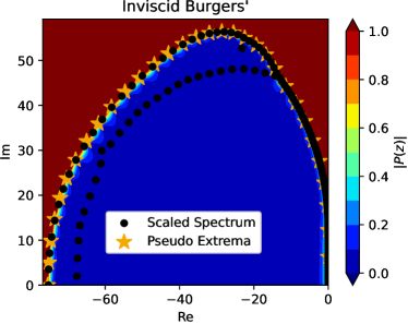
(a) Spectrum of Burgers’ Equation computed for the semidiscretization defined by item 1.

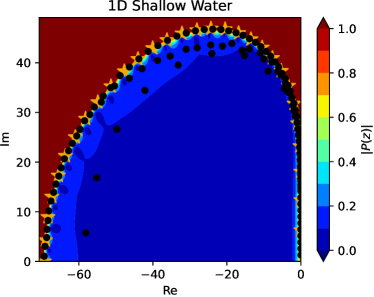
(b) Spectrum of the 1D Shallow Water Equations computed for the semidiscretization defined by item 2.

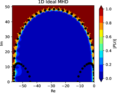
(c) Spectrum of the 1D Compressible Ideal MHD computed for the semidiscretization defined by item 3.

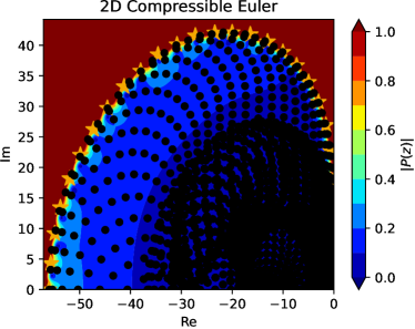
(d) Spectrum of the 2D Compressible Euler equations computed for the semidiscretization defined by item 4.

Figure 4: Collection of strictly convex spectra of nonlinear hyperbolic pdes and optimized pseudo-extrema. The spectra are scaled with the optimal timestep $\Delta t_{16,2}$ in each case.

7 Non-Convex Spectra

While a rich set of spatial discretization, equation, boundary and initial condtition combinations leads to strictly convex spectra, especially in one spatial dimension, at least equally many cases with non-convex spectra are observed. In this section, we propose two possible treatments thereof.

First, alpha shapes [78, 79] are proposed as a potentially accurate, yet more expensive candidate which come with an unknown hyperparameter. Second, we follow the previous sections and use a convex hull approach also for non-convex spectra.

7.1 Alpha Shapes

Alpha shapes [78, 79] provide a rigorous way of constructing a point enclosing shape that is potentially closer to the point set than the convex hull. Alpha shapes are parametrized by the real scalar $\alpha$ parameter that defines how close the alpha shape is shrinked to the points. For $\alpha>0$, the construction of alpha shapes can intuitively described by rolling a disk with radius $1/\alpha$ around the points and drawing a line between two points of the set whenever they are on the edge of the disk and no points are in the interior of the disk. For $\alpha=0$, the disk has infinite radius, i.e., degenerates to a straight line and the resulting shape is equivalent to the convex hull which is constructed by tilting the straight line around the points. While alpha shapes provide potentially a very accurate ansatz for the stability boundary, cf. Fig. 5 they come with two main drawbacks.

First, alpha shapes introduce a hyperparameter whose choice is not clear. While in general higher degree polynomials follow the stability boundary more closely, i.e., correspond to larger alpha values the best choice is highly dependent on the individual spectra. Furthermore, for high $\alpha$ corresponding to small radii there is always the danger of obtaining a disjoint alpha shape which is not useful in this context. Both of these issues can be in principle addressed through manual inspection, which is clearly not attractive.

Secondly, and more severely, alpha shapes provide in general only a spectrum enclosing curve $\gamma_{\alpha}(\tau):\mathbb{R}\to\mathbb{C}$, i.e., no spectrum enclosing function. This implies that for both the imaginary part (cf. (4.7)) and real part

$$\begin{split}I_{\text{Re}}\left(\tau;\sigma^{\alpha}_{S,p}\right)=\>&\text{Re}\left(\mu_{S,p}^{(j)}\right)+\frac{\text{Re}\left(\mu_{S,p}^{(j+1)}\right)-\text{Re}\left(\mu_{S,p}^{(j)}\right)}{\tau^{(j+1)}_{S,p}-\tau_{S,p}^{(j)}}\left(\tau-\tau_{S,p}^{(j)}\right),\\ &\tau_{S,p}^{(j)}\leq\tau<\tau_{S,p}^{(j+1)}\end{split}$$ (7.1)

of the pseudo-extrema interpolation has to be performed. Here, $\mu^{(j)}\in\sigma^{\alpha}$ are the eigenvalues selected as the upper part of the alpha shape with corresponding arc length parameter $0\leq\tau^{(j)}\leq 1$. This results in doubled computational costs and an overall more difficult optimization task.

Nevertheless, we stress that the general idea of distributing the pseudo-extrema with equal arc length, i.e., equal distances $\Delta\tau=\tau^{(j+1)}-\tau^{(j)},\>\forall j$ is still applicable and Algorithm 1 can be used under the appropriate changes.

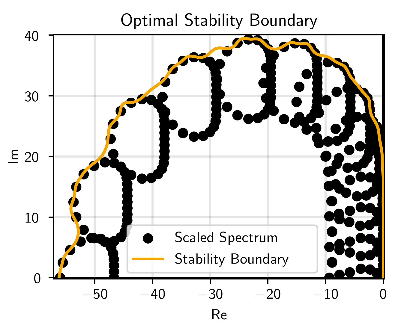
(a) $\partial\mathcal{S}_{50}$ for the scaled spectrum $\Delta t_{50,2}\sigma$.

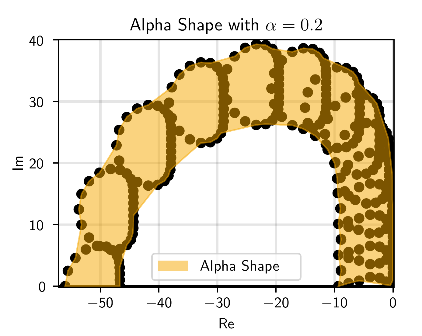
(b) Alpha shape with $\alpha=0.2$ of the scaled spectrum $\Delta t_{50,2}\sigma$.

Figure 5: Approximation of the optimal stability boundary by the contour of an alpha shape. The spectrum $\sigma$ is obtained from a dgsem discretization of the 2D linear advection equation with velocities $a_{x}=0.5,a_{y}=-0.1$ on the periodic domain $\Omega=[-1,1]^{2}$ discretized by a $6\times 6$ mesh with local polynomials of degree $3$ and Rusanov/Local Lax-Friedrichs flux.

7.2 Convex Hull Ansatz

By constructing the convex hull for non-convex spectra the framework prepared in the previous sections is recovered. Precisely, even if the hull of spectrum itself may be nonconvex, the convex hull is constructed and used as the ansatz for the initial placement of the pseudo-extrema. Using the convex hull difficulties with additional hyperparameters or the danger of disjoint alpha shapes are ruled out. This comes with the drawback that we can no longer expect to actually realize the maximum possible optimal timestep according to 4.1. Consequently, one has to indeed perform the optimization problems 5.1, 5.3 as the feasibility problems with fixed timestep will fail. Depending on the spectrum there are a priori no guarantees how efficient this approach will be. In practice, however, we find for many real-world spectra excellent results, as illustrated in the next section.

8 Optimal Stability Polynomials for Nonconvex Spectra

Here, we present results for two relevant, exemplary nonconvex spectra for which we use the convex hull-based approach.

1. Burgers’ Equation with Riemannian initial data $u_{0}(x)=\begin{cases}1.5&x<0.5\\ 0.5&x\geq 0\end{cases}$. As before, we discretize $\Omega=[0,1]$ with $64$ cells and use Godunov’s flux. At $x=0$ we fix $u(t,0)=1.5$ while at $x=1$ an outflow boundary is used. The solution is reconstructed using fourth order local polynomials. The corresponding spectrum is displayed in Fig. 6a alongside its convex hull. The convex hull is in most parts extremely close the spectrum and we thus expect maximal timesteps very close to the optimal ones according to 4.1. Indeed, for $30,60$, and $120$ degree polynomials we can realize the optimal timestep. As for the convex spectra, we display the $S=60$ case in Fig. 6a.

2. 2D compressible Euler equations: Isentropic vortex advection. The advection of an isentropic vortex is a classic, fully nonlinear testcase with known analytical solution [58, 80]. In terms of the physical parameters we use the same setup as in [38, 39, 40] which is spelled out in Section 10.2.2. The numerical scheme is composed of Rusanov/Local Lax-Friedrichs flux, second order local polynomials and 8 cells in each direction. This little resolution is required to execute the eigenvalue decomposition in reasonable time. The corresponding spectrum is shown in Fig. 6b alongside its convex hull. Similar to Burgers’ Equation, the spectrum is in most parts reasonably close to the spectrum. For $S=28$ we can realize about $97.9\%$ of the theoretically optimal timestep and for $S=56,S=112$ indeed the optimal timestep according to the linear timestep scaling 4.1.

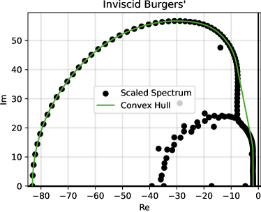
(a) Spectrum of Burgers’ equation computed for the semidiscretization as specified by item 1.

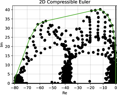
(b) Spectrum of the 2D Compressible Euler equations computed for the semidiscretization as specified by item 2.

Figure 6: Collection of nonconvex convex spectra of nonlinear hyperbolic pdes and corresponding convex hull. The spectra are scaled with the optimal timesteps $\Delta t_{S,2}$.

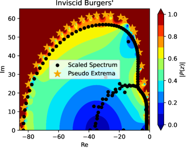
(a) Spectrum of Burgers’ Equation computed
for the semidiscretization defined by item 1.

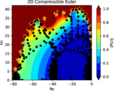
(b) Spectrum of the 2D Compressible Euler equations computed for the semidiscretization defined by item 2.

Figure 7: Collection of strictly convex spectra of nonlinear hyperbolic pdes and optimized pseudo-extrema. The spectra are scaled with the optimal timestep $\Delta t_{16,2}$ in each case.

9 Construction of Many Stage Runge-Kutta Methods

As discussed before, the primal use case of the high degree stability polynomials is the possibility to construct many-stage methods for e.g. partitioned multirate Runge-Kutta methods such as the PERK [38, 39, 44] schemes. Nevertheless, we seek to demonstrate the capabilities of the optimized stability polynomials by constructing many-stage standalone methods. Here, we limit ourselves to second order accurate methods for which the linear order constraints 2.4 imply second order convergence even in the nonlinear case, without any additional constraints [45, 6]. Furthermore, we leave the construction of ssp methods for future work and focus here on hyperbolic pdes with smooth solutions.

Due to the factorized form of the stability polynomial one can directly read-off a possible choice of the intermediate steps:

$$P_{S}(z)=1+z\widetilde{P}_{S-1}=\underbrace{1+z\left(\prod_{j=1}^{S_{\text{Real}}}\underbrace{\left(1-\frac{z}{\widetilde{r}_{j}}\right)}_{\text{Forward Euler}}\cdot\prod_{j=1}^{S_{\text{Complex}}/2}\underbrace{\left(1-\frac{z}{\widetilde{r}_{j}}\right)\left(1-\frac{z}{\widetilde{r}_{j}^{\star}}\right)}_{\text{Two-Stage Submethod}}\right)}_{\text{Forward Euler}}$$ (9.1)

Note that we group the complex-conjugated pseudo-extrema to avoid complex-valued timesteps. We focus on real timesteps since they allow easy implementation into existing codes and spare us from technical complications. Readers interested in complex-valued timesteps are pointed to [81] and references therein.

Being equipped with a stability polynomial, one has now in principle infinitely many possible choices for the actual Runge-Kutta method. It is well-known that internal stability, i.e., the propagation of round-off errors is a relevant concern for many stage explicit methods [56, 55, 82]. This issue arises also here and seems to be the major difficulty in realizing the maximum timestep.

Given the factorized form of the stability polynomial it is natural to construct Runge-Kutta methods with a sequential structure. Here, we specify the methods in modified Shu-Osher form [83, 82]

$$\boldsymbol{Y}_{k} \coloneqq v_{k}\boldsymbol{U}_{n}+\sum_{l=1}^{k-1}\big{(}\alpha_{k,l}\boldsymbol{Y}_{l}+\Delta t\beta_{k,l}\boldsymbol{F}(\boldsymbol{Y}_{l})\big{)},\quad k=1,\dots,S+1$$ (9.2a)

$$\boldsymbol{U}_{n+1} \,=\boldsymbol{Y}_{S+1}$$ (9.2b)

and set $v_{1}=1,v_{k}=0,k>1$ which implies $\boldsymbol{Y}_{1}=\boldsymbol{U}_{n}$. Following [82] we introduce the notation

$$\alpha_{1:S}|_{i,j}\coloneqq\alpha_{i,j},\quad\beta_{1:S}|_{i,j}\coloneqq\beta_{i,j}$$ (9.3)

with $\alpha_{1:S},\beta_{1:S}\in\mathbb{R}^{S\times S}$ resembling the coefficients of the intermediate stages. The parameters of the final stage are denoted via $\boldsymbol{\alpha}_{S+1},\boldsymbol{\beta}_{S+1}\in\mathbb{R}^{1\times S}$, i.e.,

$$\boldsymbol{\alpha}_{S+1}\coloneqq\begin{pmatrix}\alpha_{S+1,1}&\dots&\alpha_{S+1,S}\end{pmatrix},\quad\boldsymbol{\beta}_{S+1}\coloneqq\begin{pmatrix}\beta_{S+1,1}&\dots&\beta_{S+1,S}\end{pmatrix}$$ (9.4)

which are in the present case conveniently chosen as

$$\boldsymbol{\alpha}_{S+1}=\begin{pmatrix}1&\dots&0\end{pmatrix},\quad\boldsymbol{\beta}_{S+1}=\begin{pmatrix}0&\dots&0&z\end{pmatrix}$$ (9.5)

due to the particular representation of the stability polynomial 9.1.

The two-stage submethod (cf. 9.1) corresponding to pseudo-extrema $\widetilde{r}_{j},\widetilde{r}_{j}^{\star}$ are naturally represented via the low-storage scheme

$$\boldsymbol{Y}_{k} =\boldsymbol{Y}_{k-1}+\beta_{k,k-1}^{(j)}\boldsymbol{F}\left(\boldsymbol{Y}_{k-1}\right)$$ (9.6a)

$$\boldsymbol{Y}_{k+1} =\alpha_{k+1,k-1}^{(j)}\boldsymbol{Y}_{k-1}+\alpha_{k+1,k}^{(j)}\boldsymbol{Y}_{k}+\Delta t\left(\beta_{k+1,k-1}^{(j)}\boldsymbol{F}(\boldsymbol{U}_{k-1})+\beta_{k+1,k}^{(j)}\boldsymbol{F}(\boldsymbol{Y}_{k})\right).$$ (9.6b)

The Forward Euler steps are readily reflected by $\alpha_{k,k-1}^{(j)}=1,\beta_{k,k-1}^{(j)}=\frac{-1}{\widetilde{r}_{j}}$. To meet the stability polynomial 9.1 we have for the two-stage methods the constraints

$$\frac{-2\text{Re}(\widetilde{r}_{j})}{|\widetilde{r}_{j}|^{2}} \overset{!}{=}\alpha_{k+1,k}^{(j)}\beta_{k,k-1}^{(j)}+\beta_{k+1,k-1}^{(j)}+\beta_{k+1,k}^{(j)}$$ (9.7a)

$$\frac{1}{|\widetilde{r}_{j}|^{2}} \overset{!}{=}\beta_{k,k-1}^{(j)}\beta_{k+1,k}^{(j)}$$ (9.7b)

besides the usual requirement for consistency $\sum_{l=0}^{k-1}\alpha_{k,l}=1$ [59]. The timestamps/abscissae are computed via $\boldsymbol{c}\coloneqq(I-\alpha_{1:S})^{-1}\beta_{1:S}\boldsymbol{1}$ [82] where $\boldsymbol{1}$ denotes a column vector of ones. The ordering of the two-stage submethods, i.e., the relation of $j$ to $k$ is determined based on the accumulated $\beta$ values

$$\left\|\boldsymbol{\beta}^{(j)}_{k}\right\|_{1}=\left\|\left(\beta_{k,k-1}^{(j)},\beta_{k+1,k-1}^{(j)},\beta_{k+1,k}^{(j)}\right)\right\|_{1}.$$ (9.8)

The methods are then ordered such that $\left\|\boldsymbol{\beta}^{(j)}_{k}\right\|_{1}$ increases with $k$.

9.1 Internal Stability

For the discussion of internal stability we follow the main results derived in [82]. Under the influence of round-off errors $\boldsymbol{e}_{k}$ the modified Shu-Osher form 9.2a reads

$$\widetilde{\boldsymbol{Y}}_{k}\coloneqq v_{k}\widetilde{\boldsymbol{U}}_{n}+\sum_{l=1}^{k-1}\Big{(}\alpha_{j,l}\widetilde{\boldsymbol{Y}}_{l}+\Delta t\beta_{k,l}\boldsymbol{F}\left(\widetilde{\boldsymbol{Y}}_{l}\right)\Big{)}+\boldsymbol{e}_{k},\quad k=1,\dots,S+1$$ (9.9)

where we denote the perturbed, round-off error bearing stages by $\widetilde{\boldsymbol{Y}}_{k}$. In [82] it was shown that the defect from actually computed, perturbed solution $\widetilde{\boldsymbol{U}}_{n}$ to the true solution $\boldsymbol{U}(t_{n})$ can for linear odes be estimated as

$$\left\|\widetilde{\boldsymbol{U}}_{n+1}-\boldsymbol{U}(t_{n+1})\right\|\leq\left\|\widetilde{\boldsymbol{U}}_{n}-\boldsymbol{U}(t_{n})\right\|+\sum_{k=1}^{S+1}\left\|Q_{j}(z)\right\|\|\boldsymbol{e}_{k}\|+\mathcal{O}\left(\Delta t^{p+1}\right).$$ (9.10)

In addition to the usual truncation error $\mathcal{O}(\Delta t^{p+1})$ we have the amplification of round-off errors $\sum_{k}\|Q_{k}(z)\|\|\boldsymbol{e}_{k}\|$. Internal stability becomes a concern when both are of similar magnitude [82].

In the estimate of the error of the perturbed iterates 9.10 $Q_{j}(z)$ denote the internal stability polynomials [55, 82] which are for a method in Shu-Osher form computed as [82]

$$\boldsymbol{Q}(z;\alpha,\beta)\coloneqq(\boldsymbol{\alpha}_{S+1}+z\boldsymbol{\beta}_{S+1})\left(I-\alpha_{1:S}-z\beta_{1:S}\right)^{-1}.$$ (9.11)

For explicit methods there is no initial round-off error $\boldsymbol{e}_{1}$ [82] and it suffices to consider the internal stability polynomials starting from second stage. To estimate the potential of round-off error amplification it is customary to investigate

$$\widetilde{\mathcal{M}}(\alpha,\beta)\coloneqq\max_{z\in\mathcal{S}}\sum_{k=2}^{S+1}|Q_{k}(z;\alpha,\beta)|$$ (9.12)

which is a more precise variant of the maximum internal amplification factor proposed in [82]. For standard double precision floating point datatypes we expect the round-off errors to be $\varepsilon=\mathcal{O}\left(10^{-15}\right)$ at most, thus we expect the overall internal errors to be of order $\widetilde{\mathcal{M}}\cdot 10^{-15}$. This can then be compared to $\mathcal{O}(\Delta t^{p+1})$ yielding an approximate criterion to estimate the influence of round-off errors. Both metrics are reported for the examples considered in Section 10.

In principle, one could now set out to minimize $\widetilde{\mathcal{M}}$ over $\alpha,\beta$ under the constraints 9.7. Given that even for methods with two intermediate stages 9.6 we have $\frac{5}{2}S_{\text{Complex}}+S_{\text{Real}}$ free optimization variables and one is minimizing not only one, but $S$ polynomials at $M$ eigenvalues this is a significantly harder optimization problem than the original one 2.7. In addition, there are no immediate properties of the internal stability polynomials $Q_{j}$ available, rendering this problem practically infeasible. As an alternative, we propose a significantly cheaper heuristically motivated approach in the next section.

9.2 Internal Stability Optimization: Heuristic Approach

We begin by recalling that $\alpha_{1:S},\beta_{1:S}$ are for explicit methods strictly lower triangular, i.e., nilpotent matrices with index $S$. Consequently, the identity

$$\left(I-\alpha_{1:S}-z\beta_{1:S}\right)^{-1}=\sum_{k=0}^{S-1}\left(\alpha_{1:S}+z\beta_{1:S}\right)^{k}$$ (9.13)

holds and allows an alternative to the inversion of the typically ill-conditioned matrix. We make now the following heuristic argument: For $\alpha_{k,l}\in[0,1]$ and $|z|\sim\mathcal{O}(100)$ for the many stage methods we expect a significantly higher sensitivity of $\widetilde{M}$ with respect to $\beta_{k,l}$ than $\alpha_{k,l}$. In order to minimize $\widetilde{M}$ we thus minimize the accumulated $\beta_{k,l}$ values 9.8 for each two-stage submethod individually. For these optimization problems constraints 9.7 satisfying local minima are easily found. Note that negative $\beta_{k,l}$ are allowed here, which allow further reduction of $\widetilde{M}$ due to the increased flexibility. To illustrate this, consider the $104$ degree stability polynomial optimized for the scalar advection equation (see Section 10.1.1) for which we construct Runge-Kutta methods with non-negative and unconstrained $\beta_{k,l}$. For this case, values of $\mathcal{M}$ for grouped and non grouped pseudo-extrema (see next section) with non-negative and unconstrained $\beta_{k,l}$ are tabulated in Table 2.

9.3 Generalized Lebedev’s Idea

For the higher order dg spectra we observe a couple of pseudo-extrema near the imaginary axis with $\left|\text{Im}(\widetilde{\boldsymbol{r}}_{j})\right|\gg-\text{Re}(\widetilde{\boldsymbol{r}}_{j})$ which can lead to $\beta_{k,l}\gg 1$, which should be avoided. Similar to Lebedev’s Idea/Realization [84, 85] we group the complex conjugated pseudo-extrema with $\text{Re}(\widetilde{\boldsymbol{r}}_{j})>-0.5$ with the pseudo-extrema of largest $\left|\text{Re}(\widetilde{\boldsymbol{r}}_{j})\right|$. By staying with the two register form 9.6 we have now $13$ free parameters, three linear constraints due to $\sum_{k=0}^{j-1}\alpha_{j,k}=1$ and four nonlinear constraints which are derived similar to 9.7 by multplying out polynomials. As they are quite lengthy but readily obtained we omit them here. As for the remaining two-stage methods, we optimize $\alpha,\beta$ to minimize $\left\|\boldsymbol{\beta}^{(j)}_{k}\right\|_{1}$.

The grouping of pseudo-extrema with small and large real part has a dramatic influence on the internal stability properties. For instance, consider again the $104$ degree, second order accurate stability polynomial optimized for the scalar advection equation (see Section 10.1.1) for which we construct Runge-Kutta methods with and without grouping. Values for $\widetilde{\mathcal{M}}$ are tabulated in Table 2 highlighting the importance of the grouping. Due to this results all in the following constructed methods bear grouping of pseudo-extrema and may have negative $\beta_{k,l}$.

	$\beta_{k,l}\in\mathbb{R}_{0}^{+}$	$\beta_{k,l}\in\mathbb{R}$
No Grouping	$2.39\cdot 10^{22}$	$2.19\cdot 10^{22}$
Grouping	$7.54\cdot 10^{16}$	$1.63\cdot 10^{9}$

Table 2: Internal error amplification $\widetilde{M}$ 9.12 for different method construction paradigms.

9.4 Note on ssp Properties

It is natural to ask for ssp properties of Runge-Kutta schemes intended for the integration of (nonlinear) hyperbolic systems. Furthermore, given the representation of the method in Shu-Osher form 9.2 one can readily tell whether the method is monotonicity preserving or not. For the methods resembling the factorized form of the stability polynomial the coefficients of the last stage are chosen according to 9.5. Consequently, the ssp cofficient [59]

$$c\coloneqq\min_{k,l}\frac{\alpha_{k,l}}{\beta_{k,l}}$$ (9.14)

is due to $\alpha_{S+1,S}=0,\beta_{S+1,S}=1$ always zero, regardless of the parametrization of the intermediate stages. This implies that there exists no timestep $\Delta t>0$ such that the Runge-Kutta method is guaranteed to be monotonicity preserving. One will also need to revisit whether negative $\beta_{k,l}$ should be allowed as they demand special treatment for ssp methods [59]. The construction of many stage ssp methods is ongoing research.

10 Many-Stage Runge-Kutta Methods: Results

We present convergence studies of the many-stage Runge-Kutta methods which are constructed from the factorized form of the stability polynomial using the generalization of Lebedev’s Idea and possibly negative $\beta_{k,l}$.

10.1 Linear Problems

10.1.1 1D Advection of a Gaussian Pulse

As a first example, we consider the linear advection equation with unit transport velocity and Gaussian initial data

$$u_{t}+u_{x}=0,\quad u(x,0)=u_{0}(x)=\exp\left(\frac{-x^{2}}{0.1}\right)$$ (10.1)

on $\Omega$ = $[-5,5]$ equipped with periodic boundaries. We discretize $\Omega$ with $512$ cells and 10.1 via the dgsem with third order polynomials and Rusanov/Local Lax-Friedrichs flux implemented in Trixi.jl [64, 65, 66]. Using Trixi.jl we can generate the Jacobian using algorithmic differentiation and compute the corresponding spectrum. For this spectrum we compute the reference timestep $\Delta_{16,3}\approx 3.53\cdot 10^{-2}$ using the algorithm proposed in [35] which is then supplied to the feasibility problems 5.4 and 5.5.

We compute ten passes through the domain corresponding to final time $t_{f}=100$ with $26,52,$ and $104$ stage, third order accurate methods using the Runge-Kutta parametrization with negative $\beta$ and generalized Lebedev’s idea. The used timestep $\Delta t$, number of taken timesteps $N_{t}$, internal amplification factors $\widetilde{\mathcal{M}}$ and the order of the truncation error $\Delta t^{4}$ are reported in Table 3. The third order convergence in $L^{\infty}$-norm

$$e_{S}^{\infty}\coloneqq\left\|u^{(h,S)}(t_{f},x)-u(t_{f},x)\right\|_{\infty}$$ (10.2)

is observed until spatial discretization errors are becoming relevant, cf. Fig. 8a. In weighted $L^{1}$-norm

$$e_{S}^{1}\coloneqq\frac{1}{|\Omega|}\left\|u^{(h,S)}(t_{f},x)-u(t_{f},x)\right\|_{1}$$ (10.3)

third order convergence is observed except for the smallest timestep, as displayed in Fig. 8b. We observe that the error constant increases with stage number, which seems to be a general phenomenon for the herein constructed methods.

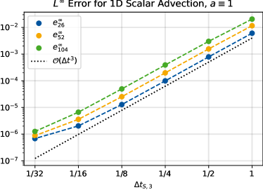
(a) $L^{\infty}$ errors for scalar advection equation.

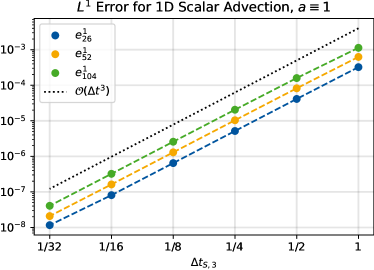
(b) Weighted $L^{1}$ errors for scalar advection equation.

Figure 8: Third order convergence in $L^{\infty},L^{1}$ for methods with 26, 52, and 104 stages optimized for the 1D scalar advection equation (10.1).

$S$	$\Delta t$	$N_{t}$	$\widetilde{\mathcal{M}}\cdot 10^{-15}$	$\Delta t^{4}$
26	$5.72\cdot 10^{-2}$	$1748$	$3.59\cdot 10^{-12}$	$1.07\cdot 10^{-5}$
52	$1.14\cdot 10^{-1}$	$874$	$1.46\cdot 10^{-9}$	$1.72\cdot 10^{-4}$
104	$2.29\cdot 10^{-1}$	$437$	$5.39\cdot 10^{-5}$	$2.75\cdot 10^{-3}$

Table 3: Results for the simulation of the 1D scalar advection equation 10.1 with three many stage optimized methods constructed using Algorithm 1. The timestep $\Delta t$ is kept constant over the $N_{t}$ timesteps, with the possible exemption of the last timestep which may be reduced in order to match the desired final time $t_{f}=100$.

10.1.2 2D Linearized Euler Equations

The linearized Euler equations with source term read in two spatial dimensions, primitive variables

$$\partial_{t}\begin{pmatrix}\rho^{\prime}\\ u^{\prime}\\ v^{\prime}\\ p^{\prime}\end{pmatrix}+\partial_{x}\begin{pmatrix}\bar{\rho}u^{\prime}+\bar{u}\rho^{\prime}\\ \bar{u}u^{\prime}+\frac{p^{\prime}}{\bar{\rho}}\\ \bar{u}v^{\prime}\\ \bar{u}p^{\prime}+c^{2}\bar{\rho}u^{\prime}\end{pmatrix}+\partial_{y}\begin{pmatrix}\bar{\rho}v^{\prime}+\bar{v}\rho^{\prime}\\ \bar{v}u^{\prime}\\ \bar{v}v^{\prime}+\frac{p^{\prime}}{\bar{\rho}}\\ \bar{v}p^{\prime}+c^{2}\bar{\rho}v^{\prime}\end{pmatrix}=\boldsymbol{s}$$ (10.4)

where $(\bar{\rho},\bar{u},\bar{v},c)=(1,1,1,1)$ denote the base state. By the method of manufactured solutions [86, 87] we set the solution to

$$\begin{pmatrix}\rho^{\prime}\\ u^{\prime}\\ v^{\prime}\\ p^{\prime}\end{pmatrix}=\begin{pmatrix}-\cos(2\pi t)\left[\sin(2\pi x)-\sin(2\pi y)\right]\\ \sin(2\pi t)\cos(2\pi x)\\ \sin(2\pi t)\cos(2\pi y)\\ -\cos(2\pi t)\left[\sin(2\pi x)-\sin(2\pi y)\right]\end{pmatrix}$$ (10.5)

with corresponding source terms

$$\boldsymbol{s}(t,x,y)=2\pi\begin{pmatrix}-\cos(2\pi t)\left[\cos(2\pi x)-\cos(2\pi y)\right]\\ \sin(2\pi t)\sin(2\pi x)\\ \sin(2\pi t)\sin(2\pi y)\\ -\cos(2\pi t)\left[\cos(2\pi x)-\cos(2\pi y)\right]\end{pmatrix}.$$ (10.6)

The linearized Euler equations 10.4 are discretized on $\Omega=[0,1]^{2}$ with $64$ elements in each direction. We employ the dgsem with fourth order local polynomials and hll [88] flux on a periodic domain. To leverage the computational costs of the eigenvalue decomposition, we compute the spectrum for a discretization with $8$ cells in each coordinate direction. For the resulting set of eigenvalues we compute the reference timestep $\Delta t_{16,2}\approx 4.53\cdot 10^{-2}$ using the algorithm proposed in [35] which is then supplied to the feasibility problems 5.4 and 5.5.

For the actual simulation on the $8$ times finer mesh we reduce the obtained timesteps accordingly. A convergence study is carried out in terms of the error in density fluctuation $\rho$ at final time $t_{f}=10.5$ and displayed in Fig. 9. We use $t_{f}=10.5$ since we observed for $t_{f}=10$ spurious convergence of higher than second order, which is a peculiarity of the employed testcase rather than a general phenomenon. Again, second order convergence is observed in $L^{\infty}$ for all timesteps. Here, we construct polynomials of degrees $32,64$, and $128$ and the corresponding methods with parametrization using potentially negative $\beta$ and the generalized Lebedev’s idea. Since the right-hand-side of the ode system (1.1b) depends also explicitly on time this example also showcases convergence of the many-stage methods for non-homogeneous problems.

In contrast to the previous example, we observe that the theoretically possible maximum stable timestep has to be reduced by factor CFL (see Table 4) for a stable simulation which we attribute to issues with internal stability. Consider for instance the $128$ stage method with $\text{CFL}=1.0$ (corresponding to an unstable simulation) with $\widetilde{\mathcal{M}}\cdot 10^{-15}\approx 7.60\cdot 10^{-2}$ while $\Delta t^{3}\approx 9.29\cdot 10^{-4}$. As discussed in [82], we observe in this case stability problems when error terms due to round off are of larger magnitude than the truncation error. For the $S=64$ stability polynomial the reduction in optimal timestep is a consequence of the optimization of the stability polynomials for the reduced spectrum, rather than related to internal stability.

$S$	$\Delta t$	CFL	$N_{t}$	$\widetilde{\mathcal{M}}\cdot 10^{-15}$	$\Delta t^{3}$
32	$1.13\cdot 10^{-2}$	$1.0$	$928$	$1.91\cdot 10^{-11}$	$1.45\cdot 10^{-6}$
64	$2.17\cdot 10^{-2}$	$0.96$	$484$	$6.30\cdot 10^{-9}$	$1.03\cdot 10^{-5}$
128	$3.67\cdot 10^{-2}$	$0.81$	$287$	$5.63\cdot 10^{-5}$	$4.94\cdot 10^{-5}$

Table 4: Results for the simulation of the 2D linearized Euler equations 10.4 with three many stage optimized methods constructed using Algorithm 1. The timestep $\Delta t$ is kept constant over the $N_{t}$ timesteps, with the possible exemption of the last timestep which may be reduced in order to match the desired final time $t_{f}=10.5$.

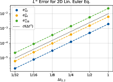
Figure 9: Second order convergence of the optimized methods with $32,64$, and $128$ stages optimized for the 2D linearized Euler equations. For each method, we reduce from the largest stable timestep $\text{CFL}\cdot\Delta t_{S,2}$.

10.2 Nonlinear Problems

10.2.1 Burgers’ Equation with Source Term

We consider Burgers’ Equation as the classic prototype equation for nonlinear hyperbolic pdes. With source term $s(t,x)$, Burgers’ Equation reads

$$\partial_{t}u+\frac{1}{2}\partial_{x}u^{2}=s.$$ (10.7)

The presence of the source term allows a convenient construction of a continuously differentiable solution $u(t,x)\in C^{1}$. This approach is known as the method of manufactured solutions [86, 87]. Here, the solution is set to

$$u(t,x)\coloneqq 2+\sin\big{(}2\pi(x-t)\big{)}$$ (10.8)

which corresponds to a simple advection of the initial condition, although this time through a nonlinear pde. Note that $u(t,x)$ is periodic on $[0,1]$ for all times $t$. The source term is then computed from the governing pde 10.7 as

$$s(t,x)\coloneqq 2\pi\cos\big{(}2\pi(x-t)\big{)}\Big{(}1+\sin\big{(}2\pi(x-t)\big{)}\Big{)}.$$ (10.9)

The spatial discretization is realized using the dgsem with third order polynomials on a $256$ element mesh $\Omega^{(h)}$ with periodic boundaries and Godunov flux [89].

Despite being effectively also only the simple advection of the initial data $u_{0}(x)$, it is now observed that internal stability limits the effectively stable timestep much more than in case of the advection equation discussed previously. This is attributed to the fact that the perturbations $\boldsymbol{e}_{j}$ do not only corrupt the stage updates (cf. 9.9), but thereby also change the point of evaluation of the Jacobian and thus the spectrum. This can have dramatic effects since the stability polynomial is only optimized for the spectrum corresponding to the unperturbed solution. This is further amplified by the lack of the ssp property of the constructed schemes. Thus, as the time integration schemes used here have no oscillation-surpressing guarantees, these do arise and further perturb the spectrum. To measure this, we compute the increase of the total variation

$$e_{\text{TV}}\coloneqq\|\boldsymbol{u}^{(h)}\left(t_{f}\right)\|_{\text{TV}}-\|\boldsymbol{u}^{(h)}\left(t_{0}\right)\|_{\text{TV}}$$ (10.10)

where the total variation semi-norm is defined as usual

$$\|\boldsymbol{u}(t)\|_{\text{TV}}\coloneqq\sum_{j}\left|u_{j+1}(t)-u_{j}(t)\right|.$$ (10.11)

For methods with $S=28,56$, and $112$ stages we observe indeed increase in total variation, cf. Table 5.

$S$	$\Delta t$	CFL	$N_{t}$	$\widetilde{\mathcal{M}}\cdot 10^{-15}$	$\Delta t^{3}$	$e_{\text{TV}}$
28	$3.67\cdot 10^{-3}$	$0.72$	$1363$	$1.41\cdot 10^{-12}$	$4.95\cdot 10^{-8}$	$1.30\cdot 10^{-2}$
56	$7.04\cdot 10^{-3}$	$0.69$	$711$	$1.39\cdot 10^{-10}$	$3.48\cdot 10^{-7}$	$5.18\cdot 10^{-2}$
112	$3.99\cdot 10^{-3}$	$0.28$	$876$	$4.79\cdot 10^{-10}$	$1.86\cdot 10^{-7}$	$6.09\cdot 10^{-3}$

Table 5: Results for the simulation of Burgers equation 10.7 with three many stage optimized methods constructed using Algorithm 1. The timestep $\Delta t$ is kept constant over the $N_{t}$ timesteps, with the possible exemption of the last timestep which may be reduced in order to match the desired final time $t_{f}=5$.

Here, the significant decrease of the optimal timestep even for methods with moderate stages is not expected to follow from issues with internal stability. Although the estimate for the perturbed approximation 9.10 is only valid for linear systems, we consider it also here as a crude estimate for the influence of internal stability. As note in table Table 5 the maximum possible timestep $\Delta t_{28,2}$ has to be decreased to $72\%$ of its theoretically possible value. As $\widetilde{M}\cdot 10^{-15}$ is still 4 orders of magnitude smaller than $\Delta t^{3}$ we do not expect the round off errors to limit the stability.

Instead, we believe that the lack of the ssp property causes the limitations in timestep. To provide reason for this, we consider ssp the third order accurate methods with variable number of stages $S_{n}=n^{2}$ proposed in [90]. For the $S=15^{2}=225$ method we have $\widetilde{M}\cdot 10^{-15}\approx 2.13\cdot 10^{-13}$ and $\Delta t^{4}\approx 5.42\cdot 10^{-8}$, i.e., similar values to the $28$ stage method constructed here. In that case, however, we have $e_{\text{TV}}\equiv 0$, as expected for the tvd time integration when applied to a smooth solution. For the schemes constructed here the spurious oscillations can even produce amplifying modes in the spectrum of the semidiscretization, i.e., move the system into an unphysical, energy-generating state. In that case, the true solution itself is unstable - this is a qualitatively different scenario to the lack of A-stability where the numerical scheme is unstable for a certain eigenvalue. For $S=28$ and $\Delta t$ from Table 5 we have for instance at $t=0.5$ an eigenvalue with $\text{Re}\left(\lambda\right)=8.57\cdot 10^{-12}$ which bears the possibility to cause the whole computation to diverge.

Nevertheless, all methods achieve second order convergence in $L^{\infty}$-norm once the oscillations vanished which is the case for $\Delta t\leq\frac{1}{4}\Delta t_{S,2}$, cf. Fig. 10a. In weighted $L^{1}$-norm (10.3) second order convergence is observed for every timestep as displayed in Fig. 10b.

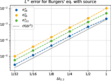
(a) $L^{\infty}$ errors for Burgers’ equation.

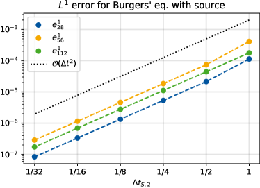
(b) Weighted $L^{1}$ errors for Burgers’ equation.

Figure 10: Second order convergence in $L^{\infty},L^{1}$ for methods optimized for Burgers’ Equation with source 10.7.

10.2.2 2D Compressible Euler Equations: Isentropic Vortex Advection

To conclude the examples, we consider the 2D compressible Euler equations

$$\partial_{t}\rho+\nabla\cdot\begin{pmatrix}\rho v_{x}\\ \rho v_{y}\end{pmatrix} =0$$ (10.12a)

$$\partial_{t}\begin{pmatrix}\rho v_{x}\\ \rho v_{y}\end{pmatrix}+\nabla\cdot\begin{pmatrix}\rho v_{x}^{2}&\rho v_{x}v_{y}\\ \rho v_{y}v_{x}&\rho v_{y}^{2}\end{pmatrix}+\nabla p =\boldsymbol{0}$$ (10.12b)

$$\partial_{t}E+\nabla\cdot\begin{pmatrix}(E+p)v_{x}\\ (E+p)v_{y}\end{pmatrix} =0$$ (10.12c)

with total energy $E=E(\rho,\boldsymbol{v},p)=\rho\left(\frac{p}{\gamma-1}+\frac{1}{2}\left(v_{x}^{2}+v_{y}^{2}\right)\right)$. As a testcase we consider the advection of an isentropic vortex [91, 80]. Here, we use similar parameters to the ones used in [39, 38]. In particular, the base state is set to

$$\rho_{\infty}=1,\quad\boldsymbol{v}_{\infty}=\begin{pmatrix}1\\ 1\end{pmatrix},\quad p_{\infty}\coloneqq\frac{\rho_{\infty}^{\gamma}}{\gamma\text{Ma}_{\infty}^{2}}$$ (10.13)

with $\text{Ma}_{\infty}=0.4$. To localize the effect of the vortex centered at $\boldsymbol{c}(t,x,y)\coloneqq\begin{pmatrix}x\\ y\end{pmatrix}-\boldsymbol{v}_{\infty}t$ the perturbations are weighted with the Gaussian $g(t,x,y)\coloneqq\exp\left(\frac{1-\|\boldsymbol{c}(t,x,y)\|_{2}^{2}}{2R^{2}}\right)$ where $R=1.5$. While the size of the vortex is governed by $R$, its intensity/strength is quantified by $I$ which is set here to $13.5$ following [39, 38]. The density is given by

$$\rho(t,x,y)=\rho_{\infty}\left(1-\frac{I^{2}M^{2}(\gamma-1)g^{2}(t,x,y)}{8\pi^{2}}\right)^{\frac{1}{\gamma-1}}$$ (10.14)

and the corresponding perturbed velocities are

$$\boldsymbol{v}(t,x,y)=\boldsymbol{v}_{\infty}+\frac{Ig(t,x,y)}{2\pi R}\boldsymbol{c}(t,x,y)$$ (10.15)

while the pressure is computed analogous to the base pressure 10.13 as

$$p(t,x,y)=\frac{\rho^{\gamma}(t,x,y)}{\gamma\text{Ma}_{\infty}^{2}}.$$ (10.16)

The advection of the vortex is simulated on $\Omega=[-10,10]^{2}$ discretized with $64\times 64$ elements, sixth order local polynomials, and HLLC Flux [92]. Final time $t_{f}$ is set to $20$ which corresponds to a full traversion of the vortex through the periodic domain. For this setup $30,60$, and $120$ degree methods of second order accuracy are constructed. As for the previous example, we observe a reduction of the theoretically stable timestep as given in Table 6 which we attribute again to the lack of ssp guarantees.

$S$	$\Delta t$	CFL	$N_{t}$	$\widetilde{\mathcal{M}}\cdot 10^{-15}$	$\Delta t^{3}$
30	$5.92\cdot 10^{-2}$	$0.79$	$338$	$1.80\cdot 10^{-12}$	$2.08\cdot 10^{-4}$
60	$9.75\cdot 10^{-2}$	$0.65$	$206$	$3.21\cdot 10^{-11}$	$9.26\cdot 10^{-4}$
120	$1.20\cdot 10^{-1}$	$0.40$	$167$	$6.50\cdot 10^{-10}$	$1.72\cdot 10^{-3}$

Table 6: Results for the simulation of the 2D compressible Euler equations 10.12 with three many stage optimized methods constructed using Algorithm 1. The timestep $\Delta t$ is kept constant over the $N_{t}$ timesteps, with the possible exemption of the last timestep which may be reduced in order to match the desired final time $t_{f}=20$.

For the $L^{\infty}$ error in density $\|\rho^{(h)}(t_{f},x,y)-\rho(t_{f},x,y)\|_{\infty}$ second order convergence is observed, until spatial discretization errors start to become significant, cf. Fig. 11.

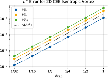
Figure 11: Second order convergence of the optimized methods with $30,60$, and $120$ stages optimized for the 2D compressible Euler equations. For each method, we reduce from the largest stable timestep $\text{CFL}\cdot\Delta t_{S,2}$.

11 Conclusions

In this work, a novel optimization approach for the generation of optimal stability polynomials for spectra of hyperbolic pdes is devised. Parametrizing the stability polynomials in terms of the herein introduced pseudo-extrema offers both a numerically stable and readily interpretable representation. The optimization approach is motivated by examining the properties of the pseudo-extrema for the proven optimal stability polynomials of first and second order for disks. These findings are directly extended to strictly convex spectra for which an optimization procedure is developed in detail. For non-convex spectra, possible remedies are discussed and optimal stability polynomials for both convex and nonconvex spectra are presented. Stability polynomials with degrees larger than 100 are constructed for a range of classical hyperbolic pdes that match the linear consistency requirements up to order three.

Equipped with high degree stability polynomials in factorized form a possible choice for the actual Runge-Kutta methods is proposed. The construction of the numerical schemes centers around minimizing the propagation and amplification of round-off errors, which can become a concern for the many stage methods. Here, methods of second order are constructed which match their designed order of accuracy for both linear and nonlinear problems. For linear problems, only internal stability might limit the theoretically possible maximum timestep while for nonlinear problems the lack of the ssp property is much more severe which spoils the effectiveness of the very high-stage methods. Nevertheless, the medium stage methods with up to, say, 64 stages are a promising candidate for stabilized methods as they allow an increase of the characteristic speeds in a simulation by a factor of four at a constant timestep compared to schemes constructed using a monomials-based approach.

Data Availability

All data generated or analysed during this study are included in this published article and its supplementary information files.

Declaration

The authors have no relevant financial or non-financial interests to disclose.

Appendix A Pseudo-Extrema of Shifted Chebyshev Polynomials

Consider the shifted Chebyshev polynomials of first kind

$$T_{S}\left(1+z/S^{2}\right)=\cos\big{(}S\arccos\left(1+z/S^{2}\right)\big{)}$$ (A.1)

providing the optimal first order stability polynomial for parabolic spectra [2, 3, 11]. It is well-known that the $S+1$ extrema of the shifted Chebyshev polynomials are on the $[-2S^{2},0]$ interval given by

$$x_{j}\coloneqq S^{2}\left(\cos\left(\frac{j\pi}{S}\right)-1\right),\quad j=0,\dots,S$$ (A.2)

where $T_{S}\left(1+x_{j}/S^{2}\right)$ attains either $+1$ or $-1$. In particular, A.2 includes the $S-1$ critical points corresponding to $j=1,\dots,S-1$ besides the extrema at the ends of the domain which correspond to $j=0$ (right end) and $j=S$ (left end).

We can rewrite the stability polynomial according to 2.10 as

$$\widetilde{P}_{S-1}(z;\widetilde{\boldsymbol{r}})=\frac{P_{S,1}(z;\widetilde{\boldsymbol{r}})-1}{z}$$ (A.3)

and seek out to determine the pseudo-extrema $\widetilde{\boldsymbol{r}}$, i.e., the roots of $\widetilde{P}_{S-1}$. Apart from $z=0$ the roots of $\widetilde{P}_{S-1}$ are given by the roots of the nominator, i.e.,

$$P_{S,1}(z;\widetilde{\boldsymbol{r}})-1=0.$$ (A.4)

For even degree $S$, $S/2+1$ roots of A.4 are given by the Chebyshev extreme points where $T_{S}\left(1+x_{j}/S^{2}\right)$ takes value $+1$:

$$\widetilde{r}_{j}=S^{2}\left(\cos\left(\frac{2j\pi}{S}\right)-1\right),\quad j=0,\dots,S/2.$$ (A.5)

We recall that the nominator of A.3 $P_{S,1}(z)-1=T_{S}\left(1+z/S^{2}\right)-1$ is a polynomial of degree $S$ in real coefficients and thus has, by the fundamental theorem of algebra, $S$ (possibly complex-conjugated) roots. As we have found already $S/2+1$ real roots it follows that the remaining $S/2-1$ roots have to be multiples of the already found ones. In particular, we have that the “outer“ roots $\widetilde{r}_{0}=-2S^{2}$ and $\widetilde{r}_{S/2}=0$ have multiplicity one, and the “interior“ roots $\widetilde{r}_{j},j=1,\dots S/2-1$ have each multiplicity two. This follows from the fact that the $\widetilde{r}_{j},j=1,\dots S/2-1$ are a subset of the critical points of $P_{S,1}(z)-1$, i.e., $\frac{\text{d}}{\text{d}z}\left(T_{S}\left(1+z/S^{2}\right)-1\right)|_{\widetilde{r}_{j}}=0,\>j=1,\dots S/2-1$.

Considering the roots of A.3 we have to be careful when it comes to $j=0$, i.e., $x_{j}=0$ since we divide by $\widetilde{r}_{j}=0$. Recalling the introduction of the lower degree polynomial (2.10) we have by construction $\widetilde{P}_{S-1}(0;\widetilde{\boldsymbol{r}})=1$. As a consequence, we have that the $S-1$ roots of the lower-degree polynomial $\widetilde{P}_{S-1}(z;\widetilde{\boldsymbol{r}})$ are given by

$$\widetilde{r}_{j}=S^{2}\left(\cos\left(\frac{2j\pi}{S}\right)-1\right),\quad j=1,\dots,S/2$$ (A.6)

where $\widetilde{r}_{S/2}$ has multiplicity one and the remaining $S/2-1$ roots have multiplicity two.

For odd degree $S$, we can follow a similar reasoning which yields that the pseudo-extrema in this case are given by

$$\widetilde{r}_{j}=S^{2}\left(\cos\left(\frac{2j\pi}{S}\right)-1\right),\quad j=1,\dots,\frac{S-1}{2}$$ (A.7)

which all have multiplicity two. This follows from the fact that for odd $S$, the extremum at the left end of the $\left[-2S^{2},0\right]$ interval of the Chebyshev polynomial is $-1$ while for even $S$, the left extremum takes value $+1$.

While these findings are for the shifted Chebyshev polynomials admittedly trivial, they generalize neatly to the known first and second order accurate optimal stability polynomials of circular/disk-like spectra, as shown in Section 3.1.

Appendix B Simulation Configurations with Strictly Convex Spectra

1. Burgers’ Equation $\partial_{t}u+\partial_{x}\frac{1}{2}u^{2}=0$ is discretized using the dgsem on $\Omega=[0,1]$ and Godunov flux [89]. The periodic domain is discretized with $64$ elements on which the solution is reconstructed using third order local polynomials. As initial condition we supply $u(t_{0},x)=2+\sin(2\pi x)$ leading to a multi-valued solution at $t=\frac{1}{2\pi}$. The spectrum is computed using the algorithmic differentiation capabilities of Trixi.jl and is displayed in Fig. 2a.

2. The Shallow Water equations with variable bottom topography $b(x)$ read in 1D

   $$\partial_{t}\begin{pmatrix}h\\ hv\end{pmatrix}+\partial_{x}\begin{pmatrix}hv\\ hv^{2}+\frac{g}{2}h^{2}\end{pmatrix}+\begin{pmatrix}0\\ gh\partial_{x}b\end{pmatrix}=\boldsymbol{0}.$$ (B.1)

   We discretize B.1 on $\Omega=[0,\sqrt{2}]$ using the dgsem with flux differencing [93, 94]. In particular, for the first component of B.1 the surface flux is approximated using the Rusanov/Local Lax-Friedrichs flux and the second component via the flux proposed in [95]. For the volume term we used the fluxes presented in [96]. $\Omega$ is discretized with $32$ cells where we use third order local polynomials to reconstruct the solution. The initial condition is in this case a moderate discontinuity:

   $$\begin{pmatrix}h(t_{0},x)\\ v(t_{0},x)\end{pmatrix}=\begin{pmatrix}-b(x)+\begin{cases}3.25&|x-0.7|>0.5\\ 4&\text{else}\end{cases}\\ \qquad\qquad\>\>\>\begin{cases}0&|x-0.7|>0.5\\ 0.1882&\text{else}\end{cases}\end{pmatrix}$$ (B.2)

   with sinusoidal bottom topography $b(x)=\sin(x)$. The corresponding spectrum is displayed in Fig. 2b.

3. The ideal compressible mhd equations considered here are of form

   $$\partial_{t}\begin{pmatrix}\rho\\ \rho v_{1}\\ \rho v_{2}\\ \rho v_{3}\\ \rho e\\ B_{1}\\ B_{2}\\ B_{3}\end{pmatrix}+\partial_{x}\begin{pmatrix}\rho v_{1}\\ \rho v_{1}^{2}+p+e_{B}-B_{1}^{2}\\ \rho v_{1}v_{2}-B_{1}B_{2}\\ \rho v_{1}v_{3}-B_{1}B_{3}\\ v_{1}(e_{v}+\gamma(\rho e-e_{v}-e_{B})+2e_{B})-B_{1}(v_{1}B_{1}+v_{2}B_{2}+v_{3}B_{3})\\ 0\\ v_{1}B_{2}-v_{2}B_{1}\\ v_{1}B_{3}-v_{3}B_{1}\end{pmatrix}=\boldsymbol{0}$$ (B.3)

   with $e_{B}\coloneqq 0.5(B_{1}^{2}+B_{2}^{2}+B_{3}^{2}),e_{v}\coloneqq\rho(v_{1}^{2}+v_{2}^{2}+v_{3}^{2}),p=(\gamma-1)(\rho e-e_{v}-e_{B})$. The solution is represented with $p=1$ local polynomials and we employ the Rusanov/Local Lax-Friedrichs flux [97]. The periodic domain $\Omega=[0,1]$ is again discretized using $32$ cells. For the initial condition we choose the Alfvén wave [98]

   $$\begin{pmatrix}\rho(t_{0},x)\\ v_{1}(t_{0},x)\\ v_{2}(t_{0},x)\\ v_{3}(t_{0},x)\\ p(t_{0},x)\\ B_{1}(t_{0},x)\\ B_{2}(t_{0},x)\\ B_{3}(t_{0},x)\end{pmatrix}=\begin{pmatrix}1\\ 0\\ 0.1\sin(2\pi x)\\ 0.1\cos(2\pi x)\\ 0.1\\ 1\\ 0.1\sin(2\pi x)\\ 0.1\cos(2\pi x)\end{pmatrix}$$ (B.4)

   and set $\gamma=\frac{5}{3}$. The spectrum for this particular configuration is shown in Fig. 2c.

4. The compressible Euler equations in two spatial dimensions are given by

   $$\partial_{t}\begin{pmatrix}\rho\\ \rho v_{1}\\ \rho v_{2}\\ \rho e\end{pmatrix}+\partial_{x}\begin{pmatrix}\rho v_{1}\\ \rho v_{1}^{2}+p\\ \rho v_{1}v_{2}\\ (\rho e+p)v_{1}\end{pmatrix}+\partial_{y}\begin{pmatrix}\rho v_{2}\\ \rho v_{1}v_{2}\\ \rho v_{2}^{2}+p\\ (\rho e+p)v_{2}\end{pmatrix}=\boldsymbol{0}$$ (B.5)

   which are represented on $\Omega=[-1,1]^{2}$ with $8$ cells per direction using second order local polynomials. Here, $p=(\gamma-1)(\rho e-0.5\rho(v_{1}^{2}+v_{2}^{2}))$ and $\gamma=1.4$. For the flux we use the hllc flux [92] and supply again periodic boundaries. The fields are initialized as

   $$\begin{pmatrix}\rho(t_{0},x)\\ v_{1}(t_{0},x)\\ v_{2}(t_{0},x)\\ p(t_{0},x)\end{pmatrix}=\begin{pmatrix}2+0.1\sin\big{(}\pi(x+y)\big{)}\\ 1\\ 1\\ \big{[}2+0.1\sin\big{(}\pi(x+y)\big{)}\big{]}^{2}\end{pmatrix}.$$ (B.6)

   The spectrum corresponding to this initial state and semidiscretization is displayed in Fig. 2d.

References

- Courant et al. [1928] R. Courant, K. Friedrichs, H. Lewy, Über die partiellen differenzengleichungen der mathematischen physik, Mathematische Annalen 100 (1928) 32–74. doi:10.1007/BF01448839.
- Franklin [1958] J. Franklin, Numerical stability in digital and analog computation for diffusion problems, Journal of Mathematics and Physics 37 (1958) 305–315.
- Guillou and Lago [1960] A. Guillou, B. Lago, Domaine de stabilité associé aux formules d’intégration numérique d’équations différentielles, a pas séparés et a pas liés. recherche de formules a grand rayon de stabilité, Ier Congr. Ass. Fran. Calcul., AFCAL (1960) 43–56.
- Saul’ev [1960] V. Saul’ev, Integration of parabolic equations by the grid method, Fizmatgiz, Moscow 13 (1960) 14–19.
- Forsythe and Wasow [1960] G. E. Forsythe, W. R. Wasow, Finite-difference methods for partial differential equations, Applied Mathematics Series, Wiley, New York, 1960.
- Wanner and Hairer [1996] G. Wanner, E. Hairer, Solving ordinary differential equations II: Stiff and differential-algebraic problems, volume 375, Springer Berlin Heidelberg New York, 1996. doi:10.1007/978-3-642-05221-7.
- Hundsdorfer and Verwer [2010] W. H. Hundsdorfer, J. G. Verwer, Numerical solution of time-dependent advection-diffusion-reaction equations, volume 33 of Springer Series in Computational Mathematics, 1 ed., Springer, 2010. doi:10.1007/978-3-662-09017-6.
- Verwer [1996] J. G. Verwer, Explicit Runge-Kutta methods for parabolic partial differential equations, Applied Numerical Mathematics 22 (1996) 359–379. doi:10.1016/S0168-9274(96)00022-0.
- Abdulle [2011] A. Abdulle, Explicit stabilized Runge-Kutta methods, Technical Report, Mathematics Institute of Computational Science and Engineering, School of Basic Sciences - Section of Mathematics EPFL Lausanne, 2011.
- Van der Houwen [1996] P. Van der Houwen, The development of Runge-Kutta methods for partial differential equations, Applied Numerical Mathematics 20 (1996) 261–272. doi:10.1016/0168-9274(95)00109-3.
- Chzao-Din [1958] Y. Chzao-Din, Some difference schemes for the solution of the first boundary value problem for linear differential equations with partial derivatives, 1958. Thesis, Moscow Stage University.
- Burrage [1985] K. Burrage, Order and stability properties of explicit multivalue methods, Applied numerical mathematics 1 (1985) 363–379. doi:10.1016/0168-9274(85)90001-7.
- Lomax [1968] H. Lomax, On the construction of highly stable, explicit, numerical methods for integrating coupled ordinary differential equations with parasitic eigenvalues, National Aeronautics and Space Administration, 1968.
- Lebedev [1993a] V. Lebedev, A new method for determining the roots of polynomials of least deviation on a segment with weight and subject to additional conditions. part i, Russian Journal of Numerical Analysis and Mathematical Modeling 8 (1993a) 195–222. doi:10.1515/rnam.1993.8.3.195.
- Lebedev [1993b] V. Lebedev, A new method for determining the roots of polynomials of least deviation on a segment with weight and subject to additional conditions. part ii, Russian Journal of Numerical Analysis and Mathematical Modeling 8 (1993b) 397–426. doi:doi.org/10.1515/rnam.1993.8.5.397.
- Van der Houwen [1977] P. J. Van der Houwen, Construction of integration formulas for initial value problems, Technical Report, Stichting Mathematisch Centrum, Amsterdam, 1977.
- Van der Houwen and Kok [1971] P. Van der Houwen, J. Kok, Numerical solution of a minimax problem, Stichting Mathematisch Centrum. Toegepaste Wiskunde (1971).
- Abdulle and Medovikov [2001] A. Abdulle, A. A. Medovikov, Second order chebyshev methods based on orthogonal polynomials, Numerische Mathematik 90 (2001) 1–18. doi:doi.org/10.1007/s002110100292.
- Riha [1972] W. Riha, Optimal stability polynomials, Computing 9 (1972) 37–43. doi:10.1007/BF02236374.
- Van der Houwen [1972] P. Van der Houwen, Explicit Runge-Kutta formulas with increased stability boundaries, Numerische Mathematik 20 (1972) 149–164. doi:10.1007/BF01404404.
- Kinnmark and Gray [1984] I. P. Kinnmark, W. G. Gray, One step integration methods with maximum stability regions, Mathematics and Computers in Simulation 26 (1984) 87–92. doi:10.1016/0378-4754(84)90039-9.
- Sonneveld and Van Leer [1984] P. Sonneveld, B. Van Leer, A minimax problem along the imaginary axis, Technical Report 4, Technische Hogeschool Delft. Onderafdeling der Wiskunde en Informatica, 1984.
- Kinnmark and Gray [1984] I. P. Kinnmark, W. G. Gray, One step integration methods of third-fourth order accuracy with large hyperbolic stability limits, Mathematics and Computers in Simulation 26 (1984) 181–188. doi:10.1016/0378-4754(84)90056-9.
- Jeltsch and Nevanlinna [1978] R. Jeltsch, O. Nevanlinna, Largest disk of stability of explicit Runge-Kutta methods, BIT Numerical Mathematics 18 (1978) 500–502.
- Owren and Seip [1990] B. Owren, K. Seip, Some stability results for explicit Runge-Kutta methods, BIT Numerical Mathematics 30 (1990) 700–706. doi:10.1007/BF01933217.
- Niegemann et al. [2012] J. Niegemann, R. Diehl, K. Busch, Efficient low-storage Runge-Kutta schemes with optimized stability regions, Journal of Computational Physics 231 (2012) 364–372. doi:10.1016/j.jcp.2011.09.003.
- Torrilhon and Jeltsch [2007] M. Torrilhon, R. Jeltsch, Essentially optimal explicit Runge-Kutta methods with application to hyperbolic–parabolic equations, Numerische Mathematik 106 (2007) 303–334. doi:10.1007/s00211-006-0059-5.
- Kennedy et al. [2000] C. A. Kennedy, M. H. Carpenter, R. Lewis, Low-storage, explicit Runge-Kutta schemes for the compressible Navier–Stokes equations, Applied Numerical Mathematics 35 (2000) 177–219. doi:10.1016/S0168-9274(99)00141-5.
- Allampalli et al. [2009] V. Allampalli, R. Hixon, M. Nallasamy, S. D. Sawyer, High-accuracy large-step explicit Runge–Kutta (hale-rk) schemes for computational aeroacoustics, Journal of Computational Physics 228 (2009) 3837–3850. doi:10.1016/j.jcp.2009.02.015.
- Toulorge and Desmet [2012] T. Toulorge, W. Desmet, Optimal Runge–Kutta schemes for discontinuous Galerkin space discretizations applied to wave propagation problems, Journal of Computational Physics 231 (2012) 2067–2091. doi:https://doi.org/10.1016/j.jcp.2011.11.024.
- Mead and Renaut [1999] J. Mead, R. Renaut, Optimal Runge–Kutta methods for first order pseudospectral operators, Journal of Computational Physics 152 (1999) 404–419. doi:https://doi.org/10.1006/jcph.1999.6260.
- Al Jahdali et al. [2021] R. Al Jahdali, R. Boukharfane, L. Dalcin, M. Parsani, Optimized explicit Runge-Kutta schemes for entropy stable discontinuous collocated methods applied to the euler and navier–stokes equations, in: AIAA Scitech 2021 Forum, 2021, p. 0633. doi:10.2514/6.2021-0633.
- Kubatko et al. [2014] E. J. Kubatko, B. A. Yeager, D. I. Ketcheson, Optimal strong-stability-preserving Runge-Kutta time discretizations for discontinuous Galerkin methods, Journal of Scientific Computing 60 (2014) 313–344. doi:10.1007/s10915-013-9796-7.
- Nasab et al. [2022] S. H. Nasab, J.-S. Cagnone, B. C. Vermeire, Optimal explicit Runge-Kutta time stepping for density-based finite-volume solver, in: AIAA SCITECH 2022 Forum, 2022, p. 1049. doi:10.2514/6.2022-1049. arXiv:https://arc.aiaa.org/doi/pdf/10.2514/6.2022-1049.
- Ketcheson and Ahmadia [2013] D. Ketcheson, A. Ahmadia, Optimal stability polynomials for numerical integration of initial value problems, Communications in Applied Mathematics and Computational Science 7 (2013) 247–271. doi:10.2140/camcos.2012.7.247.
- Vermeire et al. [2019] B. Vermeire, N. Loppi, P. Vincent, Optimal Runge–Kutta schemes for pseudo time-stepping with high-order unstructured methods, Journal of Computational Physics 383 (2019) 55–71. doi:https://doi.org/10.1016/j.jcp.2019.01.003.
- Schlottke-Lakemper et al. [2021] M. Schlottke-Lakemper, A. R. Winters, H. Ranocha, G. J. Gassner, A purely hyperbolic discontinuous Galerkin approach for self-gravitating gas dynamics, Journal of Computational Physics 442 (2021) 110467. doi:10.1016/j.jcp.2021.110467.
- Vermeire [2019] B. C. Vermeire, Paired explicit Runge-Kutta schemes for stiff systems of equations, Journal of Computational Physics 393 (2019) 465–483. doi:10.1016/j.jcp.2019.05.014.
- Hedayati Nasab and Vermeire [2022] S. Hedayati Nasab, B. C. Vermeire, Third-order paired explicit Runge-Kutta schemes for stiff systems of equations, Journal of Computational Physics 468 (2022) 111470. doi:10.1016/j.jcp.2022.111470.
- Vermeire and Hedayati Nasab [2021] B. C. Vermeire, S. Hedayati Nasab, Accelerated implicit-explicit Runge-Kutta schemes for locally stiff systems, Journal of Computational Physics 429 (2021) 110022. doi:10.1016/j.jcp.2020.110022.
- Hedayati Nasab et al. [2021] S. Hedayati Nasab, C. A. Pereira, B. C. Vermeire, Optimal Runge-Kutta stability polynomials for multidimensional high-order methods, Journal of Scientific Computing 89 (2021) 11. doi:10.1007/s10915-021-01620-x.
- Klinge and Weiner [2018] M. Klinge, R. Weiner, Strong stability preserving explicit peer methods for discontinuous Galerkin discretizations, Journal of Scientific Computing 75 (2018) 1057–1078. doi:10.1007/s10915-017-0573-x.
- Ellison and Fornberg [2021] A. C. Ellison, B. Fornberg, A parallel-in-time approach for wave-type pdes, Numerische Mathematik 148 (2021) 79–98. doi:10.1007/s00211-021-01197-5.
- Vermeire [2023] B. C. Vermeire, Embedded paired explicit Runge-Kutta schemes, Journal of Computational Physics 487 (2023) 112159. URL: https://www.sciencedirect.com/science/article/pii/S0021999123002541. doi:https://doi.org/10.1016/j.jcp.2023.112159.
- Hairer et al. [1993] E. Hairer, G. Wanner, S. P. Nørsett, Solving Ordinary Differential Equations I: Nonstiff Problems, 2 ed., Springer Berlin, Heidelberg, 1993. doi:10.1007/978-3-540-78862-1.
- Hundsdorfer et al. [2013] W. Hundsdorfer, A. Mozartova, V. Savcenco, Monotonicity Conditions for Multirate and Partitioned Explicit Runge-Kutta Schemes, Springer Berlin Heidelberg, Berlin, Heidelberg, 2013, pp. 177–195. doi:10.1007/978-3-642-33221-0_11.
- Hu et al. [1996] F. Hu, M. Y. Hussaini, J. Manthey, Low-dissipation and low-dispersion Runge-Kutta schemes for computational acoustics, Journal of Computational Physics 124 (1996) 177–191. doi:10.1006/jcph.1996.0052.
- Berland et al. [2006] J. Berland, C. Bogey, C. Bailly, Low-dissipation and low-dispersion fourth-order Runge-Kutta algorithm, Computers & Fluids 35 (2006) 1459–1463. doi:10.1016/j.compfluid.2005.04.003.
- Bernardini and Pirozzoli [2009] M. Bernardini, S. Pirozzoli, A general strategy for the optimization of Runge-Kutta schemes for wave propagation phenomena, Journal of Computational Physics 228 (2009) 4182–4199. doi:10.1016/j.jcp.2009.02.032.
- Spiteri and Ruuth [2002] R. J. Spiteri, S. J. Ruuth, A new class of optimal high-order strong-stability-preserving time discretization methods, SIAM Journal on Numerical Analysis 40 (2002) 469–491. doi:10.1137/S0036142901389025.
- Ruuth [2006] S. Ruuth, Global optimization of explicit strong-stability-preserving Runge-Kutta methods, Mathematics of Computation 75 (2006) 183–207. doi:10.1090/S0025-5718-05-01772-2.
- Sturm [1999] J. F. Sturm, Using sedumi 1.02, a matlab toolbox for optimization over symmetric cones, Optimization Methods and Software 11 (1999) 625–653. doi:10.1080/10556789908805766.
- Domahidi et al. [2013] A. Domahidi, E. Chu, S. Boyd, Ecos: An socp solver for embedded systems, in: 2013 European Control Conference (ECC), 2013, pp. 3071–3076. doi:10.23919/ECC.2013.6669541.
- Trefethen [2019] L. N. Trefethen, Approximation Theory and Approximation Practice, Extended Edition, Other Titles in Applied Mathematics, SIAM, 2019. doi:10.1137/1.9781611975949.
- Verwer et al. [1990] J. G. Verwer, W. H. Hundsdorfer, B. P. Sommeijer, Convergence properties of the Runge-Kutta-Chebyshev method, Numerische Mathematik 57 (1990) 157–178. doi:10.1007/BF01386405.
- van Der Houwen and Sommeijer [1980] P. J. van Der Houwen, B. P. Sommeijer, On the internal stability of explicit, m-stage Runge-Kutta methods for large m-values, ZAMM-Journal of Applied Mathematics and Mechanics/Zeitschrift für Angewandte Mathematik und Mechanik 60 (1980) 479–485. doi:10.1002/zamm.19800601005.
- Verwer et al. [2004] J. G. Verwer, B. P. Sommeijer, W. Hundsdorfer, Rkc time-stepping for advection–diffusion–reaction problems, Journal of Computational Physics 201 (2004) 61–79. doi:10.1016/j.jcp.2004.05.002.
- Shu and Osher [1988] C.-W. Shu, S. Osher, Efficient implementation of essentially non-oscillatory shock-capturing schemes, Journal of Computational Physics 77 (1988) 439–471. doi:10.1016/0021-9991(88)90177-5.
- Gottlieb et al. [2001] S. Gottlieb, C.-W. Shu, E. Tadmor, Strong stability-preserving high-order time discretization methods, SIAM Review 43 (2001) 89–112. doi:10.1137/S003614450036757X.
- Gottlieb et al. [2011] S. Gottlieb, D. Ketcheson, C.-W. Shu, Strong Stability Preserving Runge-Kutta and Multistep Time Discretizations, WORLD SCIENTIFIC, 2011. doi:10.1142/7498. arXiv:https://www.worldscientific.com/doi/pdf/10.1142/7498.
- Godunov and Bohachevsky [1959] S. K. Godunov, I. Bohachevsky, Finite difference method for numerical computation of discontinuous solutions of the equations of fluid dynamics, Matematičeskij sbornik 47(89) (1959) 271–306.
- Kopriva and Gassner [2010] D. A. Kopriva, G. Gassner, On the quadrature and weak form choices in collocation type discontinuous Galerkin spectral element methods, Journal of Scientific Computing 44 (2010) 136–155. doi:10.1007/s10915-010-9372-3.
- Kopriva [2009] D. A. Kopriva, Implementing spectral methods for partial differential equations: Algorithms for scientists and engineers, Scientific Computation (SCIENTCOMP), 1 ed., Springer Science & Business Media, 2009. doi:10.1007/978-90-481-2261-5.
- Ranocha et al. [2022] H. Ranocha, M. Schlottke-Lakemper, A. R. Winters, E. Faulhaber, J. Chan, G. Gassner, Adaptive numerical simulations with Trixi.jl: A case study of Julia for scientific computing, Proceedings of the JuliaCon Conferences 1 (2022) 77. doi:10.21105/jcon.00077. arXiv:2108.06476.
- Schlottke-Lakemper et al. [2021a] M. Schlottke-Lakemper, A. R. Winters, H. Ranocha, G. Gassner, A purely hyperbolic discontinuous Galerkin approach for self-gravitating gas dynamics, Journal of Computational Physics 442 (2021a) 110467. doi:10.1016/j.jcp.2021.110467. arXiv:2008.10593.
- Schlottke-Lakemper et al. [2021b] M. Schlottke-Lakemper, G. Gassner, H. Ranocha, A. R. Winters, J. Chan, Trixi.jl: Adaptive high-order numerical simulations of hyperbolic PDEs in Julia, https://github.com/trixi-framework/Trixi.jl, 2021b. doi:10.5281/zenodo.3996439.
- Vichnevetsky [1983] R. Vichnevetsky, New stability theorems concerning one-step numerical methods for ordinary differential equations, Mathematics and Computers in Simulation 25 (1983) 199–205. doi:10.1016/0378-4754(83)90092-7.
- Kinnmark [1987] I. P. Kinnmark, A principle for construction of one-step integration methods with maximum imaginary stability limits, Mathematics and Computers in Simulation 29 (1987) 87–106. doi:10.1016/0378-4754(87)90100-5.
- De Marchi et al. [2020] S. De Marchi, F. Marchetti, E. Perracchione, D. Poggiali, Polynomial interpolation via mapped bases without resampling, Journal of Computational and Applied Mathematics 364 (2020) 112347. doi:https://doi.org/10.1016/j.cam.2019.112347.
- Wächter and Biegler [2006] A. Wächter, L. T. Biegler, On the implementation of an interior-point filter line-search algorithm for large-scale nonlinear programming, Mathematical Programming 106 (2006) 25–57. doi:10.1007/s10107-004-0559-y.
- Amestoy et al. [2001] P. Amestoy, I. S. Duff, J. Koster, J.-Y. L’Excellent, A fully asynchronous multifrontal solver using distributed dynamic scheduling, SIAM Journal on Matrix Analysis and Applications 23 (2001) 15–41. doi:10.1137/S0895479899358194.
- Amestoy et al. [2019] P. Amestoy, A. Buttari, J.-Y. L’Excellent, T. Mary, Performance and scalability of the block low-rank multifrontal factorization on multicore architectures, ACM Transactions on Mathematical Software 45 (2019) 2:1–2:26. doi:10.1145/3242094.
- Karypis and Kumar [1998] G. Karypis, V. Kumar, A fast and high quality multilevel scheme for partitioning irregular graphs, SIAM Journal on scientific Computing 20 (1998) 359–392. doi:10.1137/S1064827595287997.
- Naumann et al. [2014] U. Naumann, K. Leppkes, J. Lotz, dco/C++ user guide, Technical Report, RWTH Aachen, Department of Computer Science, 2014.
- Doehring and Vigerske [2022] D. Doehring, S. Vigerske, Tell ipopt it is a feasibility problem #597, 2022. URL: https://github.com/coin-or/Ipopt/issues/597, gitHub issue.
- Liu and Nocedal [1989] D. C. Liu, J. Nocedal, On the limited memory bfgs method for large scale optimization, Mathematical Programming 45 (1989) 503–528. doi:10.1007/BF01589116.
- Doehring [2023] D. Doehring, OSPREI: Optimal stability polynomials in roots for explicit time integration, https://github.com/DanielDoehring/OSPREI, 2023. doi:10.5281/zenodo.8009493.
- Edelsbrunner et al. [1983] H. Edelsbrunner, D. Kirkpatrick, R. Seidel, On the shape of a set of points in the plane, IEEE Transactions on Information Theory 29 (1983) 551–559. doi:10.1109/TIT.1983.1056714.
- Edelsbrunner [2011] H. Edelsbrunner, Alpha shapes—a survey, Technical Report 1, IST Austria (Institute of Science and Technology Austria), 2011.
- Wang et al. [2013] Z. J. Wang, K. Fidkowski, R. Abgrall, F. Bassi, D. Caraeni, A. Cary, H. Deconinck, R. Hartmann, K. Hillewaert, H. T. Huynh, et al., High-order cfd methods: current status and perspective, International Journal for Numerical Methods in Fluids 72 (2013) 811–845. doi:10.1002/fld.3767.
- George et al. [2021] J. D. George, S. Y. Jung, N. M. Mangan, Walking into the complex plane to ’order’ better time integrators, arXiv preprint arXiv:2110.04402 (2021). doi:10.48550/arXiv.2110.04402.
- Ketcheson et al. [2014] D. I. Ketcheson, L. Lóczi, M. Parsani, Internal error propagation in explicit Runge-Kutta methods, SIAM Journal on Numerical Analysis 52 (2014) 2227–2249. doi:10.1137/130936245.
- Ferracina and Spijker [2005] L. Ferracina, M. Spijker, An extension and analysis of the Shu-Osher representation of Runge-Kutta methods, Mathematics of Computation 74 (2005) 201–219. doi:10.1090/S0025-5718-04-01664-3.
- Lebedev [1989] V. Lebedev, Explicit difference schemes with time-variable steps for solving stiff systems of equations, Soviet Journal of Numerical Analysis and Mathematical Modelling 4 (1989) 111–135. doi:10.1515/rnam.1989.4.2.111.
- Lebedev [1994] V. Lebedev, How to solve stiff systems of differential equations by explicit methods, 1 ed., CRC Press, 1994.
- Salari and Knupp [2000] K. Salari, P. Knupp, Code verification by the method of manufactured solutions, Technical Report, Sandia National Lab.(SNL-NM), Albuquerque, NM (United States), 2000. doi:10.2172/759450.
- Roache [2002] P. J. Roache, Code verification by the method of manufactured solutions, Journal of Fluids Engineering 124 (2002) 4–10. doi:10.1115/1.1436090.
- Harten et al. [1983] A. Harten, P. D. Lax, B. v. Leer, On upstream differencing and godunov-type schemes for hyperbolic conservation laws, SIAM review 25 (1983) 35–61. doi:10.1137/1025002.
- Osher [1984] S. Osher, Riemann solvers, the entropy condition, and difference, SIAM Journal on Numerical Analysis 21 (1984) 217–235. doi:10.1137/0721016. arXiv:https://doi.org/10.1137/0721016.
- Ketcheson [2008] D. I. Ketcheson, Highly efficient strong stability-preserving Runge-Kutta methods with low-storage implementations, SIAM Journal on Scientific Computing 30 (2008) 2113–2136. doi:10.1137/07070485X. arXiv:https://doi.org/10.1137/07070485X.
- Shu [1998] C.-W. Shu, Essentially non-oscillatory and weighted essentially non-oscillatory schemes for hyperbolic conservation laws, in: A. Quarteroni (Ed.), Advanced numerical approximation of nonlinear hyperbolic equations, Lecture Notes in Mathematics, Springer-Verlag Berlin Heidelberg, 1998, pp. 325–432. doi:10.1007/BFb0096351.
- Toro et al. [1994] E. F. Toro, M. Spruce, W. Speares, Restoration of the contact surface in the hll-riemann solver, Shock Waves 4 (1994) 25–34. doi:10.1007/BF01414629.
- LeFloch et al. [2002] P. G. LeFloch, J. M. Mercier, C. Rohde, Fully discrete, entropy conservative schemes of arbitraryorder, SIAM Journal on Numerical Analysis 40 (2002) 1968–1992. doi:10.1137/S003614290240069X. arXiv:https://doi.org/10.1137/S003614290240069X.
- Chen and Shu [2017] T. Chen, C.-W. Shu, Entropy stable high order discontinuous Galerkin methods with suitable quadrature rules for hyperbolic conservation laws, Journal of Computational Physics 345 (2017) 427–461. doi:https://doi.org/10.1016/j.jcp.2017.05.025.
- Fjordholm et al. [2011] U. S. Fjordholm, S. Mishra, E. Tadmor, Well-balanced and energy stable schemes for the shallow water equations with discontinuous topography, Journal of Computational Physics 230 (2011) 5587–5609. doi:https://doi.org/10.1016/j.jcp.2011.03.042.
- Wintermeyer et al. [2017] N. Wintermeyer, A. R. Winters, G. J. Gassner, D. A. Kopriva, An entropy stable nodal discontinuous Galerkin method for the two dimensional shallow water equations on unstructured curvilinear meshes with discontinuous bathymetry, Journal of Computational Physics 340 (2017) 200–242. doi:https://doi.org/10.1016/j.jcp.2017.03.036.
- Rusanov [1962] V. Rusanov, The calculation of the interaction of non-stationary shock waves and obstacles, USSR Computational Mathematics and Mathematical Physics 1 (1962) 304–320. doi:https://doi.org/10.1016/0041-5553(62)90062-9.
- Tóth [2000] G. Tóth, The div(b)=0 constraint in shock-capturing magnetohydrodynamics codes, Journal of Computational Physics 161 (2000) 605–652. doi:https://doi.org/10.1006/jcph.2000.6519.