Perceiving Longer Sequences With
Bi-Directional Cross-Attention Transformers

Abstract

We present a novel bi-directional Transformer architecture (BiXT) which scales linearly with input size in terms of computational cost and memory consumption, but does not suffer the drop in performance or limitation to only one input modality seen with other efficient Transformer-based approaches. BiXT is inspired by the Perceiver architectures but replaces iterative attention with an efficient bi-directional cross-attention module in which input tokens and latent variables attend to each other simultaneously, leveraging a naturally emerging attention-symmetry between the two. This approach unlocks a key bottleneck experienced by Perceiver-like architectures and enables the processing and interpretation of both semantics (‘what’) and location (‘where’) to develop alongside each other over multiple layers – allowing its direct application to dense and instance-based tasks alike. By combining efficiency with the generality and performance of a full Transformer architecture, BiXT can process longer sequences like point clouds or images at higher feature resolutions and achieves competitive performance across a range of tasks like point cloud part segmentation, semantic image segmentation and image classification.

1 Introduction

Much of the data we obtain when perceiving our environment can be interpreted via a division into ‘what’ and ‘where’. If we consider for example the image pictured in Figure 1 on the left, we can easily describe its content by ‘what’ we see – the building, sky and a flag. If we were to draw conclusions on a more fine-grained level though, we would likely include more specific descriptions like “lower left corner” referring to their positions within the image – the ‘where’. In other words, ‘where’ denotes the actual geometric location of the individual elements (e.gpixels) and ‘what’ the semantic entities (e.gobjects) that collectively describe the data as a whole. Note that this similarly applies to many other modalities, like point clouds or even language where we form words via letters that together have a certain meaning.

Thanks to the few structural constraints placed on the input data paired with high performance, Transformers (Vaswani et al., 2017) have shown great capabilities in extracting both ’what’ and ’where’ for a range of input modalities, giving rise to significant advances across various fields such as Natural Language Processing (Devlin et al., 2019) and Computer Vision (Dosovitskiy et al., 2021; Touvron et al., 2021, 2022). However, their success comes at the high cost of scaling quadratically in memory and time with the input length, practically prohibiting their use on larger input data like point clouds or high-resolution images when computational resources are limited.

Several approaches have since been proposed to increase their efficiency, either by changing how the computationally expensive self-attention operation is realized (Wang et al., 2020; Shen et al., 2021) or by exploiting the domain-specific structure of their data input (Parmar et al., 2018; Ho et al., 2019; Qiu et al., 2020; Tu et al., 2022). However, these approaches have a trade-off of reducing the Transformer’s performance or limiting its application to only one specific type of input (El-Nouby et al., 2021).

(a)

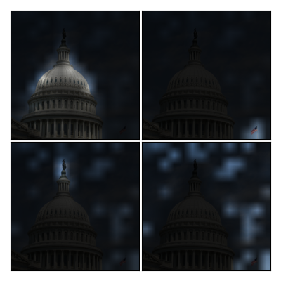
(b) Seq: lat → tok

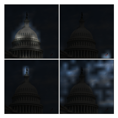
(c) Seq: lat ← tok

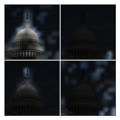
(d) Ours: lat $\longleftrightarrow$ tok

Figure 1: Emerging patterns when attending both ways. (1(a)) Input image. (1(b)) depicts the areas of the image that 4 different latents attend to, while (1(c)) inversely shows which image regions attend to these latents (transformed into the same coordinate system for ease of interpretation). (1(d)) displays which areas & latents are symmetrically attended to using our proposed bi-directional cross-attention.

In an attempt to preserve the generality by not imposing additional constraints on the input data, Jaegle et al. (2021) employ a small set of latent vectors as a bottleneck to extract the ‘what’ via one-sided (iterative) cross-attention – and require an additional decoder to draw conclusions about ‘where’ (Jaegle et al., 2022). While achieving linear complexity w.r.tthe input length, these ‘Perceiver’ architectures require between $360$ - $707$ GFLOPs to achieve around $78\%$ accuracy on ImageNet1K – results that recent ViT variants (Touvron et al., 2021, 2022) are able to obtain at a fraction of the compute. One possible explanation for this discrepancy is that the effective working memory of Perceiver architectures is strictly limited to the latents which therefore need to compensate via increased computation, whereas conventional Transformers like ViTs leverage the (larger) number of tokens across several layers. This raises an important question: Are the appealing individual properties of these two methods mutually exclusive, or can we in fact have the best of both worlds?

In this paper, we set out to affirm the latter. We demonstrate that a small set of latent vectors appropriately combined with layerwise simultaneous refinement of both input tokens and latents makes it possible to pair the high performance and architectural simplicity of ViTs with the linear scaling of Perceivers – outperforming both ViT and Perceiver in settings where compute is limited.

We start off by investigating a naïve approach: sequentially applying cross-attention to refine ‘what’ and ‘where’, one after the other. We discover that approximately symmetric attention patterns naturally emerge between latents and tokens even when both are provided with complete flexibility. In other words, for most latents (‘what’) that pay attention to particular tokens (‘where’), these tokens in turn pay attention to exactly these latents (see Figure 1 and Section 3.1). Not only does this intuitively make sense – objects need to know ‘where’ they are located in the image, and image locations need to know ‘what’ objects are located there – it more importantly offers us a unique opportunity to save FLOPs, memory and parameters.

As we will demonstrate in Section 2, this approximate symmetry means we only need to compute the attention matrix once, reducing the involved parameters by $\sim\nicefrac{{1}}{{3}}$ to facilitate an efficient bi-directional information exchange via our proposed bi-directional cross-attention. Integrated into our bi-directional cross-attention Transformer architecture (BiXT), this forms a flexible and high-performing yet efficient way to process different input modalities like images and point clouds on a variety of instance-based (e.gclassification) or dense tasks (e.gpoint cloud part segmentation) – all while scaling linearly w.r.tthe input length.

In summary, our main contributions include the following:

1. We introduce a novel bi-directional cross-attention Transformer architecture (BiXT) that scales linearly with the input size in terms of computational cost and memory consumption, allowing us to process longer sequences like point clouds or images at higher resolution.

2. We propose bi-directional cross-attention as an efficient way to establish information exchange that requires computation of the attention matrix only once and reduces the involved parameters by $\sim\nicefrac{{1}}{{3}}$, leveraging a naturally emerging symmetry in cross-attention and showing significant improvements over uni-directional iterative methods like Perceiver.

3. We analyze BiXT’s advantage of processing longer sequences across a number of tasks using different input modalities and output structures in settings with limited computational resources – with our tiny 15M parameter model achieving accuracies up to $83.1\%$ for classification on ImageNet1K without any modality-specific internal components, and performing competitively for semantic image segmentation and point cloud part segmentation even among modality-specific approaches.

4. We further provide insights into BiXT’s extendibility: Thanks to its simple and flexible design, modality-specific components can easily be incorporated in a plug-and-play fashion should the need arise – further improving results while trading off generality.

2 Perceiving via Bi-directional Cross-attention

We start this section by briefly revisiting the concept of attention before moving on to presenting our proposed bi-directional cross-attention methodology, followed by its use within our BiXT architecture (Figure 2). Please note that we define the concepts using single-head attention for brevity instead of the actually employed multi-head attention (MHA), and all methods directly generalize to MHA.

2.1 Background: The Attention Mechanism

While self-attention has recently gained great popularity through its use in the Transformer architecture (Vaswani et al., 2017), we will start from a slightly more general point of view: Given a source sequence $\mathcal{S}\in\mathbb{R}^{N\times D_{\mathcal{S}}}$ and a target sequence $\mathcal{T}\in\mathbb{R}^{M\times D_{\mathcal{T}}}\!$, attention aims to refine $\mathcal{T}$ by exhaustively discovering pairwise correlations between all elements of both sequences and integrating information from the source components of interest into the target.

Formally, $\mathcal{S}$ is linearly projected into two $D$-dimensional representations using learnable matrices – yielding a key $\boldsymbol{K}_{\mathcal{S}}\!\in\!\mathbb{R}^{N\times D}$ and value $\boldsymbol{V}_{\mathcal{S}}\!\in\!\mathbb{R}^{N\times D}$ – while $\mathcal{T}$ is projected into one $D$-dimensional representation to obtain the query $\boldsymbol{Q}_{\mathcal{T}}\in\mathbb{R}^{M\times D}\!$. These representations are then used to compute the attention-based target refinement as

$$\Delta^{\text{attn}}_{\mathcal{T}}\!=\!\text{attn}\left(\boldsymbol{Q}_{\mathcal{T}},\boldsymbol{K}_{\mathcal{S}},\boldsymbol{V}_{\mathcal{S}}\right)\!=\!\text{softmax}\!\left(\frac{\boldsymbol{Q}_{\mathcal{T}}\boldsymbol{K}_{\mathcal{S}}^{\mkern-1.5mu\mathsf{T}}}{\sqrt{D}}\right)\cdot\boldsymbol{V}_{\mathcal{S}},$$ (1)

with the scaled dot product $\bar{\boldsymbol{A}}_{\mathcal{T\!,S}}=\nicefrac{{1}}{{\sqrt{D}}}\,(\boldsymbol{Q}_{\mathcal{T}}\boldsymbol{K}_{\mathcal{S}}^{\mkern-1.5mu\mathsf{T}})\in\mathbb{R}^{M\times N}$ representing the scaled pairwise similarity between target and source elements. This concept is commonly referred to as cross-attention (CA) between target $\mathcal{T}$ and source $\mathcal{S}$. If a representation itself is to be refined given the context within, i.esource and target are identical ($\mathcal{S}\!=\!\mathcal{T}$), Equation 1 reduces to the well-known self-attention where the triplet key, query and value are all generated as a function of the same sequence elements.

Note that computing the similarity matrix $\bar{\boldsymbol{A}}_{\mathcal{T\!,S}}$ has computational complexity $\mathcal{O}(NM)$. For self-attention used in Transformers where $\mathcal{T}\!=\!\mathcal{S}$ and hence $M\!=\!N$, this yields quadratic complexity $\mathcal{O}(N^{2})$ w.r.tthe input sequence length $N$, prohibiting its use on longer sequences when computational resources are limited. On the other hand, if cross-attention is employed with a fixed sequence length $M\!=\!\text{const}\ll N$, the complexity becomes linear $\mathcal{O}(N)$.

2.2 Bi-directional Cross-attention

Reducing the complexity of attention from quadratic to linear without impairing performance or adding constraints w.r.tinput modalities is one of the main aspects of this work. We build our approach on the previously introduced notion that most perceptual data can be interpreted as ‘what’ and ‘where’ – and both need to pay attention to the other for optimal information exchange. We represent the ‘what’ via a small set of $M$ learnable latent vectors and the ‘where’ via an input-dependent sequence of $N$ tokens, respectively denoted via the subscripts ${}_{\text{lat}}$ and ${}_{\text{tok}}$ in the following and with $M\ll N$. Naïvely, one could simply apply two individual cross-attention operations sequentially – first querying information from one side and then the other by creating two query-key-value triplets. However, our analyses presented in Section 3.1 show that symmetric tendencies in the attention patterns between latents and tokens naturally emerge during training, offering a chance to further reduce the computational requirements and to increase efficiency via our bi-directional cross-attention as follows.

We start by creating reference-value pairs $\boldsymbol{R}_{\text{lat}}\!\in\!\mathbb{R}^{M\times D}\!,\boldsymbol{V}_{\text{lat}}\!\in\!\mathbb{R}^{M\times D}$ and $\boldsymbol{R}_{\text{tok}}\!\in\!\mathbb{R}^{N\times D}\!,\boldsymbol{V}_{\text{tok}}\!\in\!\mathbb{R}^{N\times D}$ via learnable linear projection from the latent vectors and tokens, respectively. Leveraging symmetry to create bi-directional information exchange, pairwise similarities between latents and tokens are then computed via a scaled dot product as

$$\bar{\boldsymbol{A}}_{\text{lat,tok}}=\left(\frac{\boldsymbol{R}_{\text{lat}}\boldsymbol{R}_{\text{tok}}^{\mkern-1.5mu\mathsf{T}}}{\sqrt{D}}\right)=\bar{\boldsymbol{A}}\,^{\mkern-1.5mu\mathsf{T}}_{\text{tok,lat}},$$ (2)

which is in turn used to obtain the attention-based refinement for both, the latents and tokens, via

$$\begin{split}&\Delta^{\text{attn}}_{\text{lat}}=\text{softmax}\!\left(\bar{\boldsymbol{A}}_{\text{lat,tok}}\right)\!\cdot\!\boldsymbol{V}_{\text{tok}}\,,\\ &\Delta^{\text{attn}}_{\text{tok}}=\text{softmax}\!\left(\bar{\boldsymbol{A}}_{\text{tok,lat}}\right)\!\cdot\!\boldsymbol{V}_{\text{lat}}.\end{split}$$ (3)

Note that in addition to providing linear scaling w.r.tto the input length $N$, Equation 2 requires evaluating the most computationally-expensive operation, namely the similarity matrix ($\mathcal{O}(MN)$), only once and allows simultaneous refinement of latents and tokens as defined in Equation 3. The implicit reuse of the references as both query and key further reduces the parameter count of the linear projection matrices by $\nicefrac{{1}}{{3}}$ compared to naïve sequential cross-attention.

2.3 BiXT – Bi-directional Cross-attention Transformers

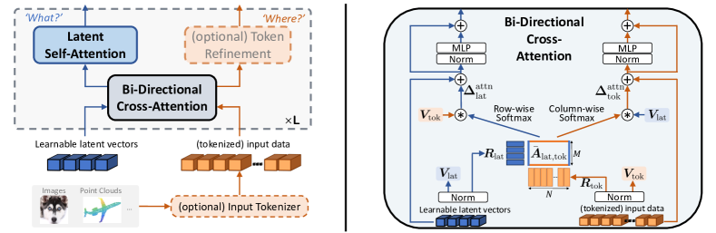
Figure 2: BiXT architecture. (left) Input data passing through one layer of our Bi-Directional Cross-Attention Transformer. (right) Internal structure of proposed efficient bi-directional cross-attention.

Figure 2 (left) illustrates the individual components that make up our BiXT architecture. BiXT is designed in a simple symmetric, ladder-like structure allowing ‘what’ (latent vectors) and ‘where’ (tokens) to simultaneously attend to and develop alongside each other – making it equally-well suited for instance-based tasks like classification and dense tasks like semantic segmentation on a variety of input modalities. We start this section with a brief overview, followed by more detailed descriptions of the individual components.

General overview.

The raw input data is first passed through a tokenization module which projects the data into an embedding sequence of length $N$ and optionally adds positional encodings, depending on the input modality and data structure. These tokens together with a fixed set of $M$ learnable latent vectors are then passed to the first layer’s bi-directional cross-attention module for efficient refinement (details depicted in Figure 2 (right) and explained below). The latents are then further refined via latent self-attention, while the tokens are either directly passed on to the next layer (default) or optionally refined by a token refinement module which could include modality-specific components. The simultaneous ladder-like refinement of ‘what’ and ‘where’ is repeated for $L$ layers, before the result is passed to task-specific output head(s). For instance-based tasks like classification, we simply average the set of latent vectors and attach a classification head to the output, while for tasks like segmentation that require outputs resembling the input data structure, the refined tokens are used.

Efficient bi-directional information exchange.

We use bi-directional cross-attention introduced in Section 2.2 to enable $M$ latents and $N$ tokens to simultaneously attend to each other in a time and memory efficient way, provided $M\ll N$. The detailed internal structure of our module is depicted in Figure 2 (right) and defined via Equations 2 and 3. Apart from the efficient bi-directional attention computation, it follows the common Transformer-style multi-head attention in terms of normalization, activations and processing via feed-forward networks (FFN) introduced by Vaswani et al. (2017) and can thus be easily implemented in modern deep learning frameworks.

Three aspects are particularly worth noting here: 1) While our bi-directional attention imposes a ‘hard’ structural constraint of symmetry on the pair-wise similarity matrix between tokens and latents as defined in Equation 2, the actual information exchange is less strict: applying the row-wise and column-wise softmax operations to obtain the actual attention maps offers a certain degree of flexibility, since adding a constant to each element in a row keeps the resulting (latent) attention map unchanged while modulating the column-wise (token) one, and vice versa. More specifically, bi-directional CA between $M$ latents and $N$ tokens has in total $M\!N\!-\!1$ degrees of freedom (dof), only $(M\!-\!1)\!\cdot\!(N\!-\!1)$ of which are shared – leaving $M\!+\!N\!-\!2$ dof that can be used by the network for the modulation of the (non-strictly-symmetric) information exchange (see Section A.3 for detailed discussion). 2) Even if the latents and tokens symmetrically attend to each other, the actual information that is transferred is created via individual value projection matrices and thus offers flexibility in terms of content. 3) While tokens cannot directly communicate with each other as is possible when using computationally expensive self-attention, this communication can still take place over two layers in our structure by using a latent vector as temporary storage in a token-latent-token sequence. Since the total number of latents is usually larger than the semantic concepts required to describe one data sample, we can expect this to be possible without impairing performance.

Latent vector refinement.

After gathering information from the tokens, we use one multi-head self-attention operation (Vaswani et al., 2017) to further refine the information stored in the latents and provide direct information exchange with a global receptive field across latents. Note that since the number of latents $M$ is much smaller than the input sequence and fixed, this operation is input-length independent and not particularly resource intensive. This step is similar to Perceiver (Jaegle et al., 2021, 2022), but we only use one instead of several self-attention operations at each layer.

Optional token refinement.

In the majority of experiments presented in this paper, we simply pass the tokens returned by the bi-directional cross-attention to the next layer. However, our architectural structure also allows to easily include additional (e.gdata-specific) modules for further refinement in a plug-n-play manner. We demonstrate examples of this in Section 3, where we add a local refinement component exploiting grid-shaped data for semantic segmentation and a data-specific hierarchical grouping module for point cloud shape classification.

Positional encodings.

We use additive sinusoidal positional encodings (Vaswani et al., 2017) to represent the structure of input data, which is more efficient than learnt encodings for variable input size. For simplicity, we follow previous works like El-Nouby et al. (2021) and create the encodings in 32 dimensions per input axis followed by a linear projection into the model’s token dimension $D$. Note that this method is applicable independent of the raw data’s dimensions and thus easily handles data ranging from 2D images to 3D or 6D point clouds.

Input tokenization. Tokenization can be performed in various ways and is the only input modality-specific component in our architecture, akin to Perceiver-IO’s input adapters (Jaegle et al., 2022). For classification experiments on image datasets like ImageNet1K (Russakovsky et al., 2015), we follow common practice and use simple linear projection as our default tokenizer to embed image patches. For point cloud data, we simply encode the 3D or 6D points directly into embedding space using our sinusoidal positional encoder. Note that we do not see any reason why BiXT should not be applicable to data beyond the scope of this paper, and any data processing module that outputs a set or sequence of embeddings could be used.

3 Experimental Evaluation

The purpose of our investigations presented in the following is twofold: 1) To provide qualitative and quantitative insights into our proposed bi-directional cross-attention and the underlying intuition of symmetry, and 2) to demonstrate how BiXT’s ability to efficiently and effectively process longer sequences positively affects various tasks. We focus the majority of our experiments around efficient architectures in the low FLOP, memory and parameter regime, and unless otherwise stated, we use BiXT with $64$ latent vectors, embedding dimension $192$ and $6$ heads for all attention modules – aka the ‘tiny’ version BiXT-Ti.

Note that where indicative results are presented, every architecture was only run once with seed 42 (no cherry picking), whereas distributional results present mean and (unbiased) standard deviation of 3 randomly seeded training runs.

Table 1: Bi-directional vsiterative attention. (1(a)) Classification accuracy on ImageNet1K. All architectures use 64 latent vectors and have been trained for 120 epochs with hyperparameters individually optimized. Architectural configurations noted in brackets. †indicates sharing of all, ‡of all but the 1st layer’s cross-attention parameters. Results reported as mean and (unbiased) std-dev over 3 randomly seeded training runs (see appendix for complete results). (1(b)) Point cloud shape classification on ModelNet40. BiXT without (naïve) and with modality-specific components in comparison to other works.

(a) ImageNet1K @ 120epochs.

	Attention	Top-1 Acc.	FLOPs	Mem.	#Param
Perceiver-like	Iterative‡ (sa5-d8)	$58.26{\scriptstyle~{}\pm~{}2.34}$	$1.58$G	$7.17$M	$19.05$M
	Iterative‡ (sa6-d7)	$54.94{\scriptstyle~{}\pm~{}5.96}$	$1.59$G	$7.23$M	$19.94$M
	Iterative† (sa6-d8)	$60.61{\scriptstyle~{}\pm~{}1.11}$	$1.82$G	$8.25$M	$22.16$M
	Iterative† (sa4-d12)	$56.03{\scriptstyle~{}\pm~{}1.02}$	$1.99$G	$9.10$M	$22.16$M
	Iterative† (sa1-d24)	$55.92{\scriptstyle~{}\pm~{}0.67}$	$1.79$G	$8.39$M	$11.93$M
Cross-Attn.	Sequential (2-way, d11)	$73.10{\scriptstyle~{}\pm~{}0.53}$	$1.66$G	$8.44$M	$14.60$M
	Apricot!20!WhiteBi-Directional  (d12)	Apricot!20!White${73.86}{\scriptstyle~{}\pm~{}0.39}$	Apricot!20!White$1.68$G	Apricot!20!White$7.86$M	Apricot!20!White$15.12$M
	Sequential (2-way, d12)	$73.79{\scriptstyle~{}\pm~{}0.32}$	$1.81$G	$9.24$M	$15.94$M
	Apricot!20!WhiteBi-Directional  (d13)	Apricot!20!White${74.10}{\scriptstyle~{}\pm~{}0.14}$	Apricot!20!White$1.82$G	Apricot!20!White$8.54$M	Apricot!20!White$16.38$M

(b) ModelNet40.

Method	OA	mAcc
Naïve, point-based
PointNet Qi et al. (2017a)	$89.2$	$86.0$
Perceiver Jaegle et al. (2021)	$85.7$	–
Apricot!20!White BiXT (naïve)	$89.6$	$86.4$
Hierarchical, point grouping, etc.
PointNet++ Qi et al. (2017b)	$90.7$	–
PointMLP Ma et al. (2022)	$94.1$	$91.3$
Apricot!20!White BiXT (+ grouping)	$92.5$	$89.7$
Apricot!20!White BiXT (+ grouping & hierarchy)	$93.1$	$90.6$

3.1 Symmetric Tendencies Emerge when Attending Both Ways

We start by investigating the intuition underlying our work: When describing data like an image by asking ‘what’ is in it and ‘where’ things are, it intuitively makes sense that these two components are tightly interconnected, and that they will inform aka pay attention to each other. To this end, we set up a naïve architecture where latent vectors first query the tokens via cross-attention (CA), followed by the tokens querying the latents (i.eusing independent query-key-value triplets), before a further refinement step of the latent information via one self-attention operation – repeated over multiple layers and trained on ImageNet1K (Russakovsky et al., 2015). When looking at the resulting attention patterns depicted in Figure 1, we discover that most latents pay attention to parts of the image representing one specific ‘entity’ like a building ((1(b)), top-left), a flag ((1(b)), top-right) or parts of the sky ((1(b)), lower-right) – supporting the notion that latent vectors represent ‘things’. More interestingly however, we discover in (1(c)) that most of these image regions (tokens) are in turn also paying attention to exactly these latent vectors – showing a roughly symmetric information exchange and providing a qualitative indication that our idea of leveraging symmetry via our bi-directional architecture might be well justified. We additionally visualize the attention patterns after replacing the naïve sequential CA through our efficient bi-directional one in (1(d)), and the results look surprisingly similar – clearly indicating that our symmetrically constrained approach can achieve similar information exchange while being significantly more efficient.

3.2 Attention – Iterative, Sequential or Bi-directional?

We aim to provide conclusive insights about the two major advantages of our proposed bi-directional attention compared to Perceiver’s iterative attention: 1) Higher performance for comparable numbers of FLOPs, and 2) Ability to optionally extend the architecture via modality-specific components. We therefore choose two tasks that have also been investigated in the Perceiver paper: Image classification on ImageNet1K (Russakovsky et al., 2015) and point cloud shape classification on ModelNet40 (Wu et al., 2015).

ImageNet classification. To provide a fair basis for comparison, we create a range of architectural configurations with iterative attention based on the insights reported by Jaegle et al. (2021). Targeting a similar FLOP count as our BiXT tiny, we experiment with different numbers of layers, varying numbers of self-attention operations per block and with sharing all CA parameters as well as all but the first layer’s (for details, see Perceiver paper and our appendix) – yielding a total of 10 architectures based on Perceiver’s iterative attention. Having optimized the hyperparameters (learning rate and schedule) for each individually, we run 3 randomly seeded training runs for the best 5 configurations and report their results after training for 120 epochs in Table 1 (1(a)) together with BiXT and the naïve sequential CA variant. It is apparent that removing the bottleneck of iterative attention significantly boosts the performance, with both BiXT and sequential CA outperforming all iterative variants by a significant margin at comparable FLOP counts. Interestingly, we find the configuration with 8 blocks and 6 self-attention layers per block (sa6-d8) to achieve best performance among the iterative variants, which aligns with the ‘best’ configuration reported by Jaegle et al. (2021).

Contrasting the two CA-based approaches with identical numbers of layers (‘d12’) demonstrates the clear advantage of our proposed bi-directional CA, requiring $\sim\!\!7\%$ fewer FLOPs, $\sim\!\!15\%$ less memory and $5\%$ fewer parameters to achieve similar results as the sequential variant. This allows BiXT to use one additional layer at matching FLOP count, consistently outperforming the naïve approach across all our experiments while being still $7\text{--}8\%$ more memory efficient.

Point cloud shape classification. To gain further quantitative insights how bi-directional attention affects processing of other modalities, we evaluate our approach on the ModelNet40 dataset (Wu et al., 2015). BiXT again clearly outperforms Perceiver in terms of overall accuracy (OA) and is even competitive to other point-based methods like the seminal PointNet (Qi et al., 2017a) (Figure 2 (1(b))). In contrast to Perceiver’s iterative attention that gathers information exclusively in the latents, BiXT’s simultaneous refinement of latents and tokens allows us to easily integrate data-specific modules for token refinement. To gauge the effect, we add the ‘affine grouping’ module from PointMLP (Ma et al., 2022) without and with hierarchical structure (i.e. point reduction). While BiXT is still outperformed by point cloud specific PointMLP, these optional modules help to boost the accuracy by up to $3.9\%$ while trading off generality.

Table 2: Classification on ImageNet1K using ‘few-FLOP’ Transformers. Note that we focus here on efficient models in the low FLOP and/or parameter regime. Perceiver architectures are included as contrast to our bi-directional attention. All methods have been trained on input resolutions of $224^{2}$, and $\uparrow\!\!384$ further fine-tuned on $384^{2}$. Note that different models may have received a different optimization effort. ^∗result reproduced as not reported in original work. ‘(conv)’ indicates the use of a convolutional tokenizer instead of a simple linear projection (see appendix for details).

Architecture	FLOPs	#Param	Acc.
‘Generalists’ – no tokenizer, no vision-specific internals
Perceiver (Jaegle et al., 2021)	$707$G	$45$M	$78.0$
Perceiver v2 (Jaegle et al., 2022)	$404$G	$42$M	$78.6$
Perceiver-IO (Jaegle et al., 2022)	$407$G	$48$M	$79.0$
‘Vanillas’ – tokenizer, but no vision-specific internals
Perceiver v2 (conv) (Jaegle et al., 2022)	$367$G	$42$M	$77.4$
Perceiver-IO (conv) (Jaegle et al., 2022)	$369$G	$49$M	$82.1$
DeiT-Ti/16 (Touvron et al., 2021)	$1.3$G	$\hphantom{1}6$M	$72.2$
DeiT3-Ti/16∗ (Touvron et al., 2022)	$1.3$G	$\hphantom{1}6$M	$75.4$
Apricot!20!White BiXT-Ti/16	$1.7$G	$15$M	$80.1$
Apricot!20!White BiXT-Ti/16 (conv)	$1.7$G	$15$M	$81.0$
Vision-specific derivatives, incl. multi-scale / pyramidal
PiT-Ti (Heo et al., 2021)	$0.7$G	$\hphantom{1}5$M	$73.0$
PiT-XS (Heo et al., 2021)	$1.4$G	$11$M	$78.1$
ViL-Ti-APE (Zhang et al., 2021)	$1.3$G	$\hphantom{1}7$M	$76.3$
ViL-Ti-RPB (Zhang et al., 2021)	$1.3$G	$\hphantom{1}7$M	$76.7$
PVTv1-Ti (Wang et al., 2021)	$1.9$G	$13$M	$75.1$
PVTv2-B1 (Wang et al., 2022)	$2.1$G	$13$M	$78.7$
XCiT-T12 (El-Nouby et al., 2021)	$1.2$G	$\hphantom{1}7$M	$77.1$
XCiT-T24 (El-Nouby et al., 2021)	$2.3$G	$12$M	$79.4$
BiFormer (Zhu et al., 2023)	$2.2$G	$13$M	$81.4$
Going finer w/ BiXT – smaller patches, larger images
Apricot!20!White BiXT-Ti/8	$4.7$G	$15$M	$81.9$
Apricot!20!White BiXT-Ti/4	$16.8$G	$15$M	$82.7$
Apricot!20!White BiXT-Ti/16 $\uparrow\!\!384$	$3.6$G	$15$M	$81.8$
Apricot!20!White BiXT-Ti/8 $\uparrow\!\!384$	$12.5$G	$15$M	$82.8$
Apricot!20!White BiXT-Ti/4 $\uparrow\!\!384$	$48.1$G	$15$M	$83.1$

3.3 Image Classification

Comparison to SOTA. Note that we focus here on efficient Transformer models in the low FLOP and/or parameter regime, with results reported in Table 2. BiXT performs favourably with default and convolutional tokenizer against the other ‘vanilla’ Transformers, outperforming both versions of DeiT by a significant margin ($6.2\,\text{--}\,11.8\%$) while being $\sim\!\!\,200\times$ more efficient than Perceiver (IO). These results are highly competitive even when compared to specialized vision-only architectures that leverage more complex pyramidal multi-scale encoding techniques, with BiXT outperforming all but one very recently proposed method (which however requires $29\%$ more FLOPs than our BiXT).

Increasing feature resolution and input size. We keep the patch size fixed to $16^{2}$ while reducing the stride of our linear patch projector to increase feature resolution (see appendix for ablation on patch sizes vsstride). Note that our BiXT/4 model can easily process $3364$ tokens per $224^{2}$ image thanks to linear scaling, boosting the top-1 accuracy to $82.7\%$. Linear scaling also lets us process larger input images more efficiently – which we investigate by fine-tuning the $224^{2}$-trained models on $384^{2}$ for 30 epochs to reduce the required computational resources. Increasing the input size allows us to further notably improve the accuracy across architectures by up to $2.1\%$, however at the expense of higher FLOP counts. Nevertheless, BiXT shows that it is possible to achieve $83.1\%$ on ImageNet using only $15$M parameters and no vision-specific internal components.

3.4 Semantic Image Segmentation

We investigate the transferability of our methods onto semantic image segmentation on the ADE20K dataset (Zhou et al., 2017). We follow common practice and integrate BiXT pretrained on ImageNet1K together with SemanticFPN (Kirillov et al., 2019) as decoder, train for 80k iterations with learning rate $6e^{-5}$ and weight decay $0.01$. We choose a batch size of 32 due to the efficiency of our model on the $512^{2}$ images. Our vanilla BiXT performs competitively against other methods with similar FLOP counts, while the more vision-specific version BiXT+LPI with local token refinement is on par with even the improved pyramidal PvTv2 and outperforms the others (Table 3).

Table 3: Semantic Segmentation on ADE20K. We again focus here on efficient models in the low FLOP and/or parameter regime. All methods trained on $512^{2}$ images.

Backbone	FLOPs	#Param	mIoU.
Using the Semantic FPN decoder (Kirillov et al., 2019)
PVTv2-B0 (Wang et al., 2022)	$25.0$G	$\hphantom{1}8$M	$37.2$
ResNet18 (He et al., 2016)	$32.2$G	$16$M	$32.9$
PVTv1-Ti (Wang et al., 2021)	$33.2$G	$17$M	$35.7$
PVTv2-B1 (Wang et al., 2022)	$34.2$G	$18$M	$42.5$
XCiT-T12 (El-Nouby et al., 2021)	$-\hphantom{G}$	$\hphantom{1}8$M	$38.1$
Apricot!20!White BiXT-Ti/16	$31.8$G	$19$M	$37.9$
Apricot!20!White BiXT-Ti/16 (+LPI from XCiT)	$32.4$G	$19$M	$42.4$
Simple linear predictor
Apricot!20!White BiXT-Ti/16	$6.4$G	$15$M	$38.4$
Apricot!20!White BiXT-Ti/8	$23.2$G	$15$M	$40.8$

Criticism on decoders & a potential alternative. Decoders like SemFPN were originally introduced for CNN-like architectures and use feature maps at multiple resolutions. Non-hierarchical Transformer architectures like BiXT thus need to downsample and up-convolve their feature maps at various stages – raising the question how this affects performance and to which extent results are caused by backbone, decoder and the compatibility of the two. To provide insights unaffected by these potential influences, we take inspiration from the recently published DINOv2 (Oquab et al., 2023) and simply use a linear layer to directly predict a segmentation map at feature resolution from the last layer’s tokens, which we then upsample using bilinear interpolation. Interestingly, our naive approach even outperforms our SemFPN variant at fewer FLOPs, indicating that more research into the suitability of these decoders with non-hierarchical architectures might be needed.

3.5 Beyond 2D Images: Point Cloud Part Segmentation

Since BiXT provides a similar generality as Perceiver regarding its input data structure but additionally allows the use of the dense, local token information, we run experiments to determine its suitability regarding the segmentation of sub-parts of a point cloud – commonly referred to as point cloud part segmentation – on the ShapeNetPart dataset (Yi et al., 2016). The naïve application of BiXT with a linear classifier directly applied to the last layer’s tokens achieves a competitive class mIoU of $83.5\%$ (instance mIoU of $85.2\%$) and outperforms other simple methods like seminal PointNet (Qi et al., 2017a), but lacks slightly behind recent more complex encoder-decoder methods like PointMLP (Ma et al., 2022) (class mIoU of $84.6\%$). Including a modality-specific token-refinement module and passing the encoded information to PointMLP’s decoder however closes the gap and lets BiXT obtain a highly competitive class mIoU of $84.7\%$ – as always trading off performance and generality. Please refer to the appendix for detailed results.

3.6 Scaling – Number of Latents & Dimensions

The majority of this paper is concerned with tiny efficient models – however, it is interesting to see whether our models follow previous Transformers in terms of scaling behavior. BiXT offers an additional degree of freedom in the number of latents. We therefore provide some insights into BiXT’s ImageNet1K performance changes for $32,64$ and $128$ latents as well as various embedding dimensions (Table 4). As expected, accuracy increases with both larger embedding dimension and number of latents – while it is worth noting that increasing the number of latents scales quadratically due to the self-attention based latent refinement. Note that we use shorter training schedules for this ablation, and results are intended to be interpreted relative to each other (not as absolute ‘best’ values). While we chose not to run excessive hyperparameter optimization and refrain from translating to very large architectures due to the large computational requirements involved, we did not observe any signs why BiXT should not behave like other Transformer architectures in terms of scaling and performance. We therefore anticipate to see similar tendencies for larger architectural variants, following the trend reported in related attention-based architectures, but leave this to future work.

Table 4: Scaling trends. Ablating the influence of varying numbers of latents and embedding dimension for ImageNet1K classification. All models trained with shorter schedule (only 300 ep) to save compute, comparisons to be performed relative to each other. Rows highlighted in gray correspond to default BiXT-Ti/16 (Acc. 80.1) from Table 2.

	#Latents	Acc. (%)	FLOPs	Mem	#Param
$\boldsymbol{D\!=\!192}$	32	$77.44$	$1.30$G	$5.80$M	$15.12$M
	Black!10!White64	Black!10!White$78.55$	Black!10!White$1.68$G	Black!10!White$7.86$M	Black!10!White$15.12$M
	128	$79.17$	$2.47$G	$12.44$M	$15.13$M
	Emb. Dim	Acc. (%)	FLOPs	Mem	#Param
$\boldsymbol{\mathrm{\#Latents}\!=\!64}$	128	$73.56$	$0.78$G	$5.24$M	$6.82$M
	160	$77.09$	$1.19$G	$6.55$M	$10.56$M
	Black!10!White192	Black!10!White$78.55$	Black!10!White$1.68$G	Black!10!White$7.86$M	Black!10!White$15.12$M
	224	$79.66$	$2.26$G	$9.18$M	$20.49$M
	256	$80.49$	$2.92$G	$10.49$M	$26.68$M
	288	$80.66$	$3.67$G	$11.80$M	$33.69$M
	320	$81.06$	$4.51$G	$13.11$M	$41.50$M

3.7 Limitations

Our results obtained from the investigation of iterative vsbi-directional attention in Section 3.2 clearly indicate that bi-directional attention is advantageous in a number of settings, including finely tokenized images of up to $7056$ tokens. However, it is worth noting that by simultaneously refining the tokens alongside the latents, BiXT does not decouple the model’s depth from the input and output, unlike Perceiver models (Jaegle et al., 2021). Therefore, very deep BiXT variants might potentially face difficulties in settings of attending to extremely long sequences like raw pixels of large images paired with limited compute and memory. However, we suspect most such scenarios to benefit from some form of preprocessing via a modality-specific input tokenizer, similar to the input-adapter-based concept used in Jaegle et al. (2022) – shifting most applications again into regions where BiXT performs effectively and efficiently.

4 Related work

The introduction of Transformers by Vaswani et al. (2017) has helped self-attention to significantly gain in popularity, despite its caveat of scaling quadratically in computational time and memory with input length. Their flexibility regarding input modality and success in Natural Language Processing (NLP) (Devlin et al., 2019) and Computer Vision (CV) (Dosovitskiy et al., 2021; Touvron et al., 2021, 2022) prompted a series of works targeting more efficient versions.

Approximating the attention matrix via low-rank factorization has been employed across NLP (Katharopoulos et al., 2020; Wang et al., 2020; Song et al., 2021), CV (Chen et al., 2018; Zhu et al., 2019; Li et al., 2019) and others (Choromanski et al., 2021), essentially avoiding the explicit computation through associativity, estimating a set of bases or using sampling – usually at the expense of performance. Others proposed to use tensor formulations (Ma et al., 2019; Babiloni et al., 2020) or exploit the input data structure (Parmar et al., 2018; Ho et al., 2019; Qiu et al., 2020; El-Nouby et al., 2021) under the umbrella of sparsity, however limiting their use to only one specific input modality.

The line of work closest related to ours are ‘memory-based approaches’ which employ some form of global memory to allow indirect interaction between local tokens. Beltagy et al. (2020) propose to compose various local windowed patterns (sliding, dilated) with global attention on few ‘pre-selected’ and task-specific input locations for NLP tasks, while its vision derivative (Zhang et al., 2021) provides global memory as tokens within a vision-pyramid architecture and employs four different pairwise attention operations combined with several sets of global tokens that are discarded at certain stages, introducing rather high architectural complexity. Ainslie et al. (2020) additionally investigate the encoding of structured NLP inputs, whereas Zaheer et al. (2020) propose a hand-crafted mix of random, window and global attention to sparsify and thus reduce attention complexity. Zhu et al. (2023) route information between selected tokens in a directed graph to achieve sparsity and skip computation in regions deemed irrelevant. Yao et al. (2023) in turn use cross-attention-based dual-blocks for efficiency but combine these with merging-blocks that cast attention over the entire concatenated token sequence, introducing a shared representation space and preventing linear scaling. While these ideas of indirect local token communication via a shared global memory align with ours, BiXT realizes this goal in a much simpler and modality-independent manner when compared to the mix of highly modality-specific components, attention patterns and strategies involved in these works. Preserving generality w.r.tthe input, Lee et al. (2019) use a set of learnable ‘inducing points’ via cross-attention to query input data, while the recent Perceiver architectures (Jaegle et al., 2021, 2022) similarly use a fixed set of latents to query input data – yet none offers the efficient simultaneous refinement of latents and tokens realized in our BiXT.

5 Conclusion

In this paper, we have presented a novel bi-directional cross-attention Transformer architecture (BiXT) for which computational cost and memory consumption scale linearly with input size, by leveraging a naturally emerging symmetry in two-way cross-attention that aligns with common intuition and has been empirically validated in this work. By allowing the ‘what’ (latent variables) and ‘where’ (input tokens) to attend to each other simultaneously and develop alongside throughout the architectural stages, BiXT combines Perceiver’s linear scaling with full Transformer architectures’ high performance in a best-of-both-worlds approach. The ability to process longer sequences paired with the ease to integrate further domain-specific token refinement modules helps BiXT to perform competitively on a number of point cloud and vision tasks, and to outperform comparable methods on ImageNet1K in the low-FLOP regime.

Impact Statement

This paper presents work whose goal is to advance the field of machine learning and in particular to increase the efficiency of Transformer models to allow higher accuracy without increasing FLOPs. There are many potential societal and ethical consequences of large-scale machine learning and its applications, but these are applicable to the entire field and not specific to our proposed architecture. Our approach aims to reduce the computational cost of Transformer models, which makes these models more accessible to users with lower-end computing systems; this democratization of AI can have positive or negative social consequences. Reducing the computational costs of Transformer models reduces their energy consumption and therefore their impact on the environment; however, these benefits may be offset if users take advantage of the increased efficiency of our approach to implement more or larger models.

Appendix A BiXT – General Aspects and Insights

A.1 Code and Reproducibility

We implemented our models in PyTorch (Paszke et al., 2019) using the timm library, and will release all code and pretrained models. We further made use of the mmsegmentation library (Contributors, 2020) for the semantic segmentation experiments. Point cloud experiments were built on the publicly released code base from Ma et al. (2022).

A.2 Complexity Analysis

The complexity of BiXT is dominated by the bi-directional cross-attention, in particular by a) the matrix multiplication to compute the similarity matrix and b) the two matrix multiplications to compute the refined outputs. Using the previously specified embedding dimension $D$, $N$ tokens and $M$ latent vectors, multiplication a) involves matrices of shape $M\!\times\!D,D\!\times\!N$ with result $M\!\times\!N$, and the two multiplications b) involve matrices of shape $M\!\times\!N,N\!\times\!D$ with result $M\!\times\!D$ and $N\!\times\!M,M\!\times\!D$ with result $N\!\times\!D$. The overall complexity per layer is thus $\mathcal{O}(MND)=\mathcal{O}(N)$ and linear in the size of the input $N$.

A.3 Bi-Directional Attention and Degrees of Freedom

In this section, we discuss the degrees of freedom (dof) inherent to our bi-directional cross-attention and provide some further insights into why the information exchange between latents and tokens is less restricted than might at first be expected. It is worth noting that there might be cases where the approximate symmetry that motivates our approach does not clearly emerge when using a naïve sequential method. Even in these cases, we however found our method to still consistently provide a net benefit across all experiments. We conjecture that multiple aspects contribute to this effect, one of which is that even though a ‘hard’ structural symmetry constraint is imposed on the pair-wise similarity matrix, the actual attention matrices obtained after row- and column-wise softmax have additional non-shared degrees of freedom which can be used to modulate the information exchange. We discuss this in the following in more detail. (Another helpful aspect could be that having an additional layer due to BiXT’s higher efficiency can compensate for additionally required non-symmetric processing, and information exchange can also be realized across multiple layers via e.ga token-latent-token sequence.)

TLDR: Bi-directional cross-attention between $M$ latents and $N$ tokens has in total $M\!N\!-\!1$ dof, only $(M\!-\!1)\!\cdot\!(N\!-\!1)$ of which are shared – leaving $M\!+\!N\!-\!2$ dof that can be used by the network for the modulation of the (non-strictly-symmetric) information exchange.

Gentle introduction. For ease of understanding, we start from a vector $\bar{\boldsymbol{v}}\in\mathbb{R}^{N}$ and apply the softmax operation to obtain $\boldsymbol{v}=\text{softmax}(\bar{\boldsymbol{v}})$. Given that all entries $v_{i}$ of this vector have to sum to $1$ due to the applied softmax operation, $\boldsymbol{v}$ has $N\!-\!1$ dof. This can also be interpreted as “adding a constant to all elements of $\bar{\boldsymbol{v}}$ doesn’t change $\boldsymbol{v}$”.

Uni-directional cross-attention. Let us now consider the pair-wise similarity matrix $\bar{\boldsymbol{A}}_{\mathcal{T\!,S}}$ between target $\mathcal{T}$ and source $\mathcal{S}$ as introduced in Section 2.1. Casting uni-directional attention between $M$ latents and $N$ tokens to refine the latents, we obtain $\boldsymbol{A}_{\text{lat},\text{tok}}=\text{softmax}(\bar{\boldsymbol{A}}_{\text{lat},\text{tok}})\in\mathbb{R}^{M\times N}$ with the softmax applied row-wise – resulting in $M\!\cdot\!(N\!-\!1)$ dof as visualized in Figure A1 1(a)). Likewise, computing the attention matrix $\boldsymbol{A}_{\text{tok},\text{lat}}\in\mathbb{R}^{N\times M}$ between tokens and latents using a different set of key and query vectors yields $N\!\cdot\!(M\!-\!1)$ dof, which is visualized in its transposed form in Figure A1 1(b)).
→ Therefore, sequentially applying two uni-directional cross-attention operations on two individual pair-wise similarity matrices provides a total of $2MN\!-\!M\!-\!N$ dof.

Bi-directional cross-attention. Unlike the sequential approach, our proposed bi-directional cross-attention uses the same pair-wise similarity matrix and obtains the attention matrices via row- and column-wise softmax. This can be interpreted as overlaying both operations and their respective degrees of freedom, and is visualized in Figure A1 1(c)). As demonstrated by the shaded area, both softmax operations ‘share’ a total of $(M\!-\!1)\!\cdot\!(N\!-\!1)$ dofs. With the row-wise softmax yielding $M\!\cdot\!(N\!-\!1)$ dof and the column-wise softmax $N\!\cdot\!(M\!-\!1)$ dof, this results in a total of $MN\!-\!1$ dof – where the ‘1’ can be interpreted as “adding the same constant to all elements pre-softmax doesn’t change the result”. Note however that while adding the same constant to all elements of a row (pre-softmax) does not affect the results after the row-wise softmax, it does change the column-wise one. Therefore, the non-overlapping areas in Figure A1 1(c)) can be interpreted as the dof that are unique to the attention maps obtained via row- or column-wise softmax, and can be used to modulate the resulting information flow to better accommodate potential deviations from symmetry.
→ Bi-directional cross-attention uses the same pairwise similarity matrix to obtain both attention maps and therefore has a total of $MN\!-\!1$ dof, $(M\!-\!1)\!\cdot\!(N\!-\!1)$ of which are shared and $M\!+\!N\!-\!2$ are unique.

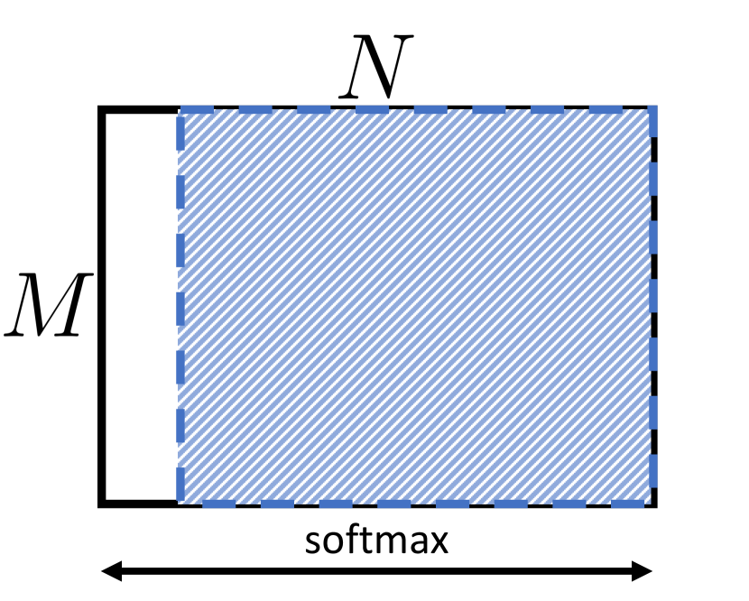
(a) uni-directional, row-wise

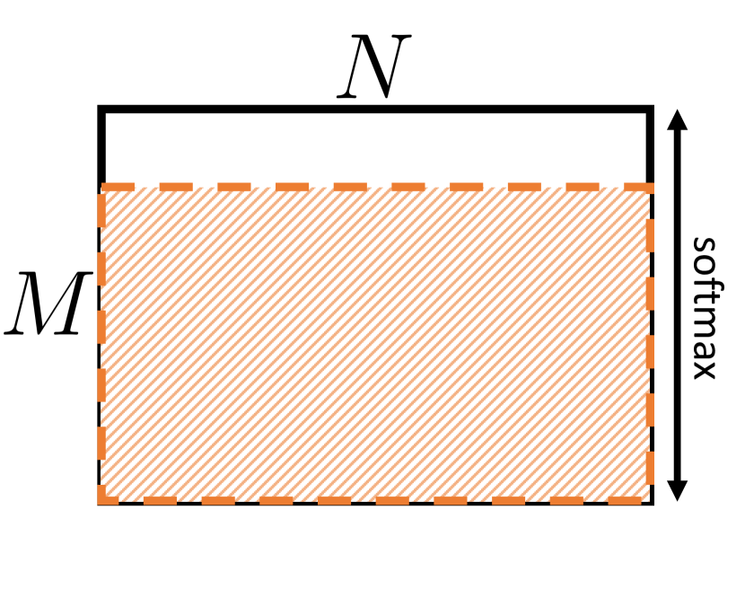
(b) uni-directional, column-wise

(c) bi-directional, row- & column-wise

Figure A1: Degrees of Freedom. (1(a)) Row-wise softmax for uni-directional cross-attention, based on matrix $\in\mathbb{R}^{M\times N}$ with $M\!\cdot(N\!-\!1)$ degrees of freedom. (1(b)) Column-wise softmax for uni-directional cross-attention, based on matrix $\in\mathbb{R}^{M\times N}$ with $N\!\cdot(M\!-\!1)$ degrees of freedom. (1(c)) Row- and column-wise softmax for our proposed bi-directional cross-attention, using the same matrix $\in\mathbb{R}^{M\times N}$ with $MN\!-\!1$ degrees of freedom.

A.4 Types of Attention – Additional Results and Further Explanations

An extended list of the results stated in Section 3.2 are presented in Table A1. Note that we performed an individual sweep over a set of learning rates for each individual architecture – usually starting at $4e^{-3}$ and lowering until stable training occurred. We then used these results to pick the best 5 architectural variants and training schemes, and ran them for an additional 2 random seeds. Note that all architectural variants, including BiXT and the sequential one have only been run in this setup for a total of maximum 3 runs, and no cherry-picking of results occurred for any of the architectures. Note that we have also tried stepped schedulers with the schedule proposed in the original Perceiver paper (Jaegle et al., 2021), but resorted back to using the cosine since it showed equal or superior results.

To contrast the sequential attention to our default BiXT with 12 layers (d12) on a matching FLOP level, the sequential version uses only 11 layers (d11) due to its higher complexity per layer. This is due to the fact that our bi-directional cross-attention only requires 4 instead of 6 projection matrices ($2\!\times\![R,V]$ vs. $2\!\times\![Q,K,V]$) and only computes the attention matrix once (instead of twice). The hereby saved FLOPs (as well as parameters and memory) can then be spent on additional layers, further improving results. Architectures with one more layer each show the same trend.

In other words, by holding FLOP and/or memory requirements constant, we consistently observe a net benefit with our bi-directional attention in terms of accuracy throughout our experiments. We empirically found that it additionally improved robustness/consistency across different parameter initializations (seeds), which can be seen by the slightly smaller standard deviations of the bi-directional variants.

Table A1: Architectural variants using iterative attention & cross-attention parameter sharing. Classification accuracy on the ImageNet1K dataset for varying types of attention. All architectures use 64 latent vectors and have been trained for 120 epochs with hyperparameters individually optimized. Cross-attention parameter sharing schemes: ^†indicates sharing of all, ^‡of all but the 1^st layer’s cross-attention parameters. Architectural configurations noted in brackets. Three randomly seeded runs were performed for the ‘best’ architectures (judged by their performance on seed = 42), and mean and (unbiased) standard deviation are reported. One randomly seeded run reported for all other architectures.

Attention type	Acc.@1 (%)	Acc.@5 (%)	FLOPs	Mem.	#Param
Iterative† (sa5-d8)	$57.51$	$80.61$	$1.58$G	$7.17$M	$18.61$M
Iterative† (sa6-d7)	$58.86$	$81.53$	$1.59$G	$7.23$M	$19.50$M
Iterative† (sa6-d8)	$60.61{\scriptstyle~{}\pm~{}1.11}$	$82.75{\scriptstyle~{}\pm~{}0.68}$	$1.82$G	$8.25$M	$22.16$M
Iterative† (sa4-d12)	$56.03{\scriptstyle~{}\pm~{}1.02}$	$79.38{\scriptstyle~{}\pm~{}0.80}$	$1.99$G	$9.10$M	$22.16$M
Iterative† (sa1-d22)	$56.09$	$79.36$	$1.64$G	$7.70$M	$11.04$M
Iterative† (sa1-d24)	$55.92{\scriptstyle~{}\pm~{}0.67}$	$79.33{\scriptstyle~{}\pm~{}0.52}$	$1.79$G	$8.39$M	$11.93$M
Iterative‡ (sa5-d8)	$58.26{\scriptstyle~{}\pm~{}2.34}$	$81.02{\scriptstyle~{}\pm~{}1.76}$	$1.58$G	$7.17$M	$19.05$M
Iterative‡ (sa6-d7)	$54.94{\scriptstyle~{}\pm~{}5.96}$	$78.39{\scriptstyle~{}\pm~{}4.69}$	$1.59$G	$7.23$M	$19.94$M
Iterative‡ (sa6-d8)	$58.23$	$80.95$	$1.82$G	$8.25$M	$22.61$M
Iterative‡ (sa4-d12)	$56.35$	$79.64$	$1.99$G	$9.10$M	$22.61$M
Sequential (2-way, d11)	$73.10{\scriptstyle~{}\pm~{}0.53}$	$91.05{\scriptstyle~{}\pm~{}0.28}$	$1.66$G	$8.44$M	$14.60$M
Sequential (2-way, d12)	$73.79{\scriptstyle~{}\pm~{}0.32}$	$91.48{\scriptstyle~{}\pm~{}0.15}$	$1.81$G	$9.24$M	$15.94$M
Apricot!20!White Bi-Directional (d12)	${73.86}{\scriptstyle~{}\pm~{}0.39}$	$91.55{\scriptstyle~{}\pm~{}0.14}$	$1.68$G	$7.86$M	$15.12$M
Apricot!20!White Bi-Directional (d13)	${74.10}{\scriptstyle~{}\pm~{}0.14}$	$91.61{\scriptstyle~{}\pm~{}0.12}$	$1.82$G	$8.54$M	$16.38$M

A.5 More Detailed Discussion of Most-recent Related Work

The two most-recent related methods, DualViT (Yao et al., 2023) and BiFormer (Zhu et al., 2023), are again discussed in slightly more detail here:

DualViT (Yao et al., 2023). DualViT’s dual block used in the early layers of their architecture does indeed show similarity to the naïve solution of sequential cross-attention, but is distinctly different from our bi-directional approach as it does not leverage any symmetry. Importantly, their multi-stage pyramidal vision-only architecture uses a large number of ‘merging blocks/layers’ (between 9 - 24) which cast full self-attention over the concatenated sequence of latents and tokens. This prevents linear scaling and also introduces a shared embedding space of latent vectors and tokens through the use of the same key-query-value projection matrices – whereas our architecture keeps those separate (aligned with the presented ’what’ and ’where’ analogy and the level of information they represent) and scales linearly with respect to the input length.

BiFormer (Zhu et al., 2023). BiFormer follows the common trend for vision-only approaches and employs a pyramidal structure. In contrast to previous work, the authors reduce the computational complexity through routing information between selected tokens via a directed graph, thus achieving sparsity to skip computation of certain regions that are deemed ‘irrelevant’. While this is a very neat way of dynamically reducing complexity, it is distinctly different from our approach and does not achieve true linear scaling.

Appendix B Further Details on ImageNet1K Experiments

This section outlines further details regarding our image classification experiments conducted on the ImageNet dataset (Russakovsky et al., 2015).

B.1 Model Configurations and Training Details

Hyperparameter choice for the default ImageNet experiments: BiXT with 64 latents, 12 layers, embedding dimension for latents and tokens $192$ paired with $6$ heads (head dimension $32$) – learning rate $2.5e^{-3}$, weight decay $0.05$ and lambc optimizer, as well as cosine learning rate scheduler with linear warmup; stochastic dropout on self-attention and cross-attention $0.1$ for all tiny models. Apart from these, we directly apply the augmentation and training proposed by Touvron et al. (2022). Our models have been trained between 300 (ablations) and 800 epochs on one or several A100 GPUs. Note that we did not conduct an extensive hyperparameter search, and we expect results to potentially improve if done so.

Finetuning on images of size $384\times 384$ was performed for 30 epochs using a batch size of 512 and an initial learning rate of $2.5e^{-5}$ with cosine decline, starting from the model trained on $224\times 224$ images. We found empirically that increasing the stochastic dropout during finetuning to $0.2$ can help to improve the results, and we hence use this as default value for our finetuning experiments.

B.2 Ablating Patch Size for Fixed Sequence Lengths in Image Classification

In this section, we investigate whether lowering the patch size to increase the resolution of the resulting feature maps is actually the most-suited way – or whether simply reducing the stride and thus creating tokens that originate from overlapping patches yield better results. Our experiments on image classification using the ImageNet1k (Russakovsky et al., 2015) dataset with models using varying patch sizes and strides to keep the sequence lengths fixed show that the originally introduced and commonly used patch size of $16\times 16$ pixels seems to be a good fit when using no overlapping patches (Table A2). Interestingly, we find that even when we increase the feature resolution and thus choose smaller strides, a patch size of $16\times 16$ still yields best results across our experiments. One potential reason is that patch boundaries are randomly chosen and objects in images do naturally not match these boundaries, so that information has to be exchanged – whereas slight overlaps might ease this to some extent. Another potential reason for this behaviour is that significantly decreasing the patch size reduces the input information per patch, with an $8^{2}$ RGB patch having a total of $192$ channels, exactly matching the tiny embedding dimension. Smaller patches however would create a significant null space, which might be an additional reason for better performance when using larger patches.

Table A2: Varying patch sizes for fixed sequence lengths. ImageNet1k classification results for varying patch sizes are presented for three fixed sequence lengths (realised via stride). All models have been trained for 300 epochs using the same (default) hyperparameters and input images of size $224\times 224$. Best results for each sequence length is highlighted in bold.

Seq. length	$196$ ($14\times 14$)		$784$ ($28\times 28$)			$3136$ ($56\times 56$)
Patch size	$32\times 32$	$16\times 16$	$32\times 32$	$16\times 16$	$8\times 8$	$16\times 16$	$8\times 8$	$4\times 4$
Acc. (%)	$77.50$	$\mathbf{78.13}$	$79.90$	$\mathbf{79.92}$	$79.36$	$\mathbf{80.95}$	$80.75$	$79.56$
FLOPs	$1.77$G	$1.68$G	$5.05$G	$4.71$G	$4.62$G	$16.81$G	$16.46$G	$16.38$G
Mem	$7.27$M	$7.23$M	$20.25$M	$20.25$M	$20.25$M	$72.18$M	$72.18$M	$72.18$M
#Param	$15.56$M	$15.11$M	$15.56$M	$15.12$M	$15.01$M	$15.12$M	$15.01$M	$14.98$M

B.3 Convolutional Tokenizer

In addition to our default linearly-projecting tokenizer, we report results using a convolutional tokenizer as BiXT-Ti/16 (conv) in Table 2. This tokenizer follows El-Nouby et al. (2021) and consists of a stack of four {conv - Batch Norm - GeLU} groups, using $3\times 3$ convs with stride 1 and sequentially encoding the input channels into the specified embedding dimension $D$ (via $\nicefrac{{D}}{{8}},\nicefrac{{D}}{{4}},\nicefrac{{D}}{{2}},D$).

B.4 Token Refinement via Local Patch Interaction (XCiT)

We integrate a slightly modified version of the ‘LPI’ module from El-Nouby et al. (2021) together with their convolutional tokenizer for our vision-specific image segmentation experiments. Our LPI module consists of two depth-wise convolutional layers (3x3) with Layer Normalization (instead of the original Batch Normalization) and a GELU non-linearity in between. For further details, please refer to the original paper.

Appendix C Further Details on Point Cloud Experiments

C.1 Training and Evaluation Details

Note that we do not use any voting strategy or other multi-scale augmentation and simply follow the training regime of PointMLP (Ma et al., 2022) for most of our experiments. We use a standard BiXT architecture for the ‘naïve’ point cloud experiments as well as the ones using simple grouping – and reduce our architecture to $4$ layers when using the decoder for part segmentation and the hierarchical approach for shape classification – paired with 32 and 24 neighbours, respectively (which are the default values used in other works like PointMLP).

C.2 Detailed Results for Point Cloud Part Segmentation

The detailed results of our experiments conducted on the ShapeNetPart dataset (Yi et al., 2016) are reported in the form of class intersection over union (IoU) and instance IoU in Table A3, together with the individual results for all object classes.

Table A3: Point cloud part segmentation on ShapeNetPart (Yi et al., 2016). Reported are the class IoU and instance IoU for BiXT and PointMLP (Ma et al., 2022). Note that we only compare here to PointMLP due to investigating the use of their grouping module and decoder within BiXT.

Method	Cls.	Inst.	aero-	bag	cap	car	chair	ear-	guitar	knife	lamp	laptop	motor-	mug	pistol	rocket	skate-	table
	mIoU	mIoU	plane					phone					bike				board
PointNet	$80.4$	$83.7$	$83.4$	$78.7$	$82.5$	$74.9$	$89.6$	$73.0$	$91.5$	$85.9$	$80.8$	$95.3$	$65.2$	$93.0$	$81.2$	$57.9$	$72.8$	$80.6$
PointMLP	$84.6$	$86.1$	$83.5$	$83.4$	$87.5$	$80.5$	$90.3$	$78.2$	$92.2$	$88.1$	$82.6$	$96.2$	$77.5$	$95.8$	$85.4$	$64.6$	$83.3$	$84.3$
Apricot!20!White BiXT  (naïve)	$83.5$	$85.1$	$83.9$	$81.4$	$91.5$	$79.0$	$89.5$	$76.2$	$91.9$	$87.3$	$79.3$	$95.8$	$73.1$	$95.0$	$84.2$	$63.7$	$80.4$	$83.5$
Apricot!20!White BiXT  (EncDec)	$84.7$	$86.0$	$84.4$	$82.7$	$86.3$	$80.9$	$90.2$	$80.1$	$92.1$	$87.8$	$82.3$	$95.9$	$78.1$	$95.9$	$84.9$	$67.0$	$82.4$	$83.9$

Appendix D Visualization of Latent-Token Attention

To provide some additional qualitative insights into the bi-directional attention that is cast within BiXT, we provide three sets of attention maps overlaid onto the input image:

• Figure A2: The attention maps of the four latent vectors presented in Figure 1(1(d)) for all layers throughout the BiXT tiny architecture (layer 1, top-left to layer 12, bottom-right).

• Figure A3 The attention maps of all latent vectors (64 in this case) for the final layer of our BiXT tiny architecture.

• Figure A4 The attention maps of all latent vectors (64 in this case) for the second-last layer of our BiXT tiny architecture.

Figure A2: Attention across layers. Bi-directional attention maps for the four selected tokens presented in Figure 1(1(d)) across all layers: Starting with first layer on top left, ending with last layer (layer 12) on the bottom right. Displayed are the mean attention maps averaged across the heads of BiXT tiny with 64 latents.

Figure A3: Attention maps of final layer. Bi-directional cross-attention maps of all 64 latent vectors of the final layer (layer 12) of our BiXT tiny architecture.

Figure A4: Attention maps of penultimate layer. Bi-directional cross-attention maps of all 64 latent vectors of the second-last layer (layer 11) of our BiXT tiny architecture.

References

- Ainslie et al. (2020) Ainslie, J., Ontanon, S., Alberti, C., Cvicek, V., Fisher, Z., Pham, P., Ravula, A., Sanghai, S., Wang, Q., and Yang, L. Etc: Encoding long and structured inputs in transformers. In Proceedings of the 2020 Conference on Empirical Methods in Natural Language Processing (EMNLP), pp. 268–284, 2020.
- Babiloni et al. (2020) Babiloni, F., Marras, I., Slabaugh, G., and Zafeiriou, S. Tesa: Tensor element self-attention via matricization. In Proceedings of the IEEE/CVF Conference on Computer Vision and Pattern Recognition, pp. 13945–13954, 2020.
- Beltagy et al. (2020) Beltagy, I., Peters, M. E., and Cohan, A. Longformer: The long-document transformer. arXiv preprint arXiv:2004.05150, 2020.
- Chen et al. (2018) Chen, Y., Kalantidis, Y., Li, J., Yan, S., and Feng, J. A2-nets: Double attention networks. Advances in Neural Information Processing Systems, 31, 2018.
- Choromanski et al. (2021) Choromanski, K. M., Likhosherstov, V., Dohan, D., Song, X., Gane, A., Sarlos, T., Hawkins, P., Davis, J. Q., Mohiuddin, A., Kaiser, L., et al. Rethinking attention with performers. In International Conference on Learning Representations, 2021.
- Contributors (2020) Contributors, M. MMSegmentation: Openmmlab semantic segmentation toolbox and benchmark. https://github.com/open-mmlab/mmsegmentation, 2020.
- Devlin et al. (2019) Devlin, J., Chang, M.-W., Lee, K., and Toutanova, K. Bert: Pre-training of deep bidirectional transformers for language understanding. In Proceedings of the 2019 Conference of the North American Chapter of the Association for Computational Linguistics: Human Language Technologies, Volume 1 (Long and Short Papers), pp. 4171–4186, 2019.
- Dosovitskiy et al. (2021) Dosovitskiy, A., Beyer, L., Kolesnikov, A., Weissenborn, D., Zhai, X., Unterthiner, T., Dehghani, M., Minderer, M., Heigold, G., Gelly, S., Uszkoreit, J., and Houlsby, N. An image is worth 16x16 words: Transformers for image recognition at scale. In International Conference on Learning Representations, 2021.
- El-Nouby et al. (2021) El-Nouby, A., Touvron, H., Caron, M., Bojanowski, P., Douze, M., Joulin, A., Laptev, I., Neverova, N., Synnaeve, G., Verbeek, J., and Jegou, H. XCiT: Cross-covariance image transformers. In Advances in Neural Information Processing Systems, 2021.
- He et al. (2016) He, K., Zhang, X., Ren, S., and Sun, J. Deep residual learning for image recognition. In Proceedings of the IEEE Conference on Computer Vision and Pattern Recognition, pp. 770–778, 2016.
- Heo et al. (2021) Heo, B., Yun, S., Han, D., Chun, S., Choe, J., and Oh, S. J. Rethinking spatial dimensions of vision transformers. In Proceedings of the IEEE/CVF International Conference on Computer Vision, pp. 11936–11945, 2021.
- Ho et al. (2019) Ho, J., Kalchbrenner, N., Weissenborn, D., and Salimans, T. Axial attention in multidimensional transformers. arXiv preprint arXiv:1912.12180, 2019.
- Jaegle et al. (2021) Jaegle, A., Gimeno, F., Brock, A., Vinyals, O., Zisserman, A., and Carreira, J. Perceiver: General perception with iterative attention. In International Conference on Machine Learning, pp. 4651–4664. PMLR, 2021.
- Jaegle et al. (2022) Jaegle, A., Borgeaud, S., Alayrac, J.-B., Doersch, C., Ionescu, C., Ding, D., Koppula, S., Zoran, D., Brock, A., Shelhamer, E., et al. Perceiver io: A general architecture for structured inputs & outputs. In International Conference on Learning Representations, 2022.
- Katharopoulos et al. (2020) Katharopoulos, A., Vyas, A., Pappas, N., and Fleuret, F. Transformers are rnns: Fast autoregressive transformers with linear attention. In International Conference on Machine Learning, pp. 5156–5165. PMLR, 2020.
- Kirillov et al. (2019) Kirillov, A., Girshick, R., He, K., and Dollár, P. Panoptic feature pyramid networks. In Proceedings of the IEEE/CVF Conference on Computer Vision and Pattern Recognition, pp. 6399–6408, 2019.
- Lee et al. (2019) Lee, J., Lee, Y., Kim, J., Kosiorek, A., Choi, S., and Teh, Y. W. Set transformer: A framework for attention-based permutation-invariant neural networks. In International Conference on Machine Learning, pp. 3744–3753. PMLR, 2019.
- Li et al. (2019) Li, X., Zhong, Z., Wu, J., Yang, Y., Lin, Z., and Liu, H. Expectation-maximization attention networks for semantic segmentation. In Proceedings of the IEEE/CVF International Conference on Computer Vision, pp. 9167–9176, 2019.
- Ma et al. (2019) Ma, X., Zhang, P., Zhang, S., Duan, N., Hou, Y., Zhou, M., and Song, D. A tensorized transformer for language modeling. Advances in Neural Information Processing Systems, 32, 2019.
- Ma et al. (2022) Ma, X., Qin, C., You, H., Ran, H., and Fu, Y. Rethinking network design and local geometry in point cloud: A simple residual mlp framework. In International Conference on Learning Representations, 2022.
- Oquab et al. (2023) Oquab, M., Darcet, T., Moutakanni, T., Vo, H., Szafraniec, M., Khalidov, V., Fernandez, P., Haziza, D., Massa, F., El-Nouby, A., et al. Dinov2: Learning robust visual features without supervision. arXiv preprint arXiv:2304.07193, 2023.
- Parmar et al. (2018) Parmar, N., Vaswani, A., Uszkoreit, J., Kaiser, L., Shazeer, N., Ku, A., and Tran, D. Image transformer. In International Conference on Machine Learning, pp. 4055–4064. PMLR, 2018.
- Paszke et al. (2019) Paszke, A., Gross, S., Massa, F., Lerer, A., Bradbury, J., Chanan, G., Killeen, T., Lin, Z., Gimelshein, N., Antiga, L., Desmaison, A., Kopf, A., Yang, E., DeVito, Z., Raison, M., Tejani, A., Chilamkurthy, S., Steiner, B., Fang, L., Bai, J., and Chintala, S. Pytorch: An imperative style, high-performance deep learning library. In Advances in Neural Information Processing Systems, pp. 8024–8035. 2019.
- Qi et al. (2017a) Qi, C. R., Su, H., Mo, K., and Guibas, L. J. Pointnet: Deep learning on point sets for 3d classification and segmentation. In Proceedings of the IEEE Conference on Computer Vision and Pattern Recognition, pp. 652–660, 2017a.
- Qi et al. (2017b) Qi, C. R., Yi, L., Su, H., and Guibas, L. J. Pointnet++: Deep hierarchical feature learning on point sets in a metric space. Advances in Neural Information Processing Systems, 30, 2017b.
- Qiu et al. (2020) Qiu, J., Ma, H., Levy, O., Yih, W.-t., Wang, S., and Tang, J. Blockwise self-attention for long document understanding. In Findings of the Association for Computational Linguistics: EMNLP 2020, pp. 2555–2565, 2020.
- Russakovsky et al. (2015) Russakovsky, O., Deng, J., Su, H., Krause, J., Satheesh, S., Ma, S., Huang, Z., Karpathy, A., Khosla, A., Bernstein, M., et al. Imagenet large scale visual recognition challenge. International Journal of Computer Vision, 115(3):211–252, 2015.
- Shen et al. (2021) Shen, Z., Zhang, M., Zhao, H., Yi, S., and Li, H. Efficient attention: Attention with linear complexities. In Proceedings of the IEEE/CVF Winter Conference on Applications of Computer Vision, pp. 3531–3539, 2021.
- Song et al. (2021) Song, K., Jung, Y., Kim, D., and Moon, I.-C. Implicit kernel attention. In Proceedings of the AAAI Conference on Artificial Intelligence, volume 35, pp. 9713–9721, 2021.
- Touvron et al. (2021) Touvron, H., Cord, M., Douze, M., Massa, F., Sablayrolles, A., and Jégou, H. Training data-efficient image transformers & distillation through attention. In International Conference on Machine Learning, pp. 10347–10357. PMLR, 2021.
- Touvron et al. (2022) Touvron, H., Cord, M., and Jégou, H. Deit iii: Revenge of the vit. In European Conference on Computer Vision, pp. 516–533. Springer, 2022.
- Tu et al. (2022) Tu, Z., Talebi, H., Zhang, H., Yang, F., Milanfar, P., Bovik, A., and Li, Y. Maxvit: Multi-axis vision transformer. In European Conference on Computer Vision, pp. 459–479, 2022.
- Vaswani et al. (2017) Vaswani, A., Shazeer, N., Parmar, N., Uszkoreit, J., Jones, L., Gomez, A. N., Kaiser, Ł., and Polosukhin, I. Attention is all you need. Advances in Neural Information Processing Systems, 30, 2017.
- Wang et al. (2020) Wang, S., Li, B. Z., Khabsa, M., Fang, H., and Ma, H. Linformer: Self-attention with linear complexity. arXiv preprint arXiv:2006.04768, 2020.
- Wang et al. (2021) Wang, W., Xie, E., Li, X., Fan, D.-P., Song, K., Liang, D., Lu, T., Luo, P., and Shao, L. Pyramid vision transformer: A versatile backbone for dense prediction without convolutions. In Proceedings of the IEEE/CVF International Conference on Computer Vision, pp. 568–578, 2021.
- Wang et al. (2022) Wang, W., Xie, E., Li, X., Fan, D.-P., Song, K., Liang, D., Lu, T., Luo, P., and Shao, L. Pvt v2: Improved baselines with pyramid vision transformer. Computational Visual Media, 8(3):415–424, 2022.
- Wu et al. (2015) Wu, Z., Song, S., Khosla, A., Yu, F., Zhang, L., Tang, X., and Xiao, J. 3d shapenets: A deep representation for volumetric shapes. In Proceedings of the IEEE Conference on Computer Vision and Pattern Recognition, pp. 1912–1920, 2015.
- Yao et al. (2023) Yao, T., Li, Y., Pan, Y., Wang, Y., Zhang, X.-P., and Mei, T. Dual vision transformer. IEEE transactions on pattern analysis and machine intelligence, 2023.
- Yi et al. (2016) Yi, L., Kim, V. G., Ceylan, D., Shen, I.-C., Yan, M., Su, H., Lu, C., Huang, Q., Sheffer, A., and Guibas, L. A scalable active framework for region annotation in 3d shape collections. ACM Transactions on Graphics (ToG), 35(6):1–12, 2016.
- Zaheer et al. (2020) Zaheer, M., Guruganesh, G., Dubey, K. A., Ainslie, J., Alberti, C., Ontanon, S., Pham, P., Ravula, A., Wang, Q., Yang, L., et al. Big bird: Transformers for longer sequences. Advances in Neural Information Processing Systems, 33:17283–17297, 2020.
- Zhang et al. (2021) Zhang, P., Dai, X., Yang, J., Xiao, B., Yuan, L., Zhang, L., and Gao, J. Multi-scale vision longformer: A new vision transformer for high-resolution image encoding. arXiv preprint arXiv:2103.15358, 2021.
- Zhou et al. (2017) Zhou, B., Zhao, H., Puig, X., Fidler, S., Barriuso, A., and Torralba, A. Scene parsing through ade20k dataset. In Proceedings of the IEEE Conference on Computer Vision and Pattern Recognition, pp. 633–641, 2017.
- Zhu et al. (2023) Zhu, L., Wang, X., Ke, Z., Zhang, W., and Lau, R. W. Biformer: Vision transformer with bi-level routing attention. In Proceedings of the IEEE/CVF Conference on Computer Vision and Pattern Recognition (CVPR), pp. 10323–10333, June 2023.
- Zhu et al. (2019) Zhu, Z., Xu, M., Bai, S., Huang, T., and Bai, X. Asymmetric non-local neural networks for semantic segmentation. In Proceedings of the IEEE/CVF International Conference on Computer Vision, pp. 593–602, 2019.