Vacancy-Induced Topological Fano Resonance in Kane-Mele Nanoribbons: Design, Control, and Sensing Applications

Abstract

The concept of topological Fano resonance, characterized by an ultrasharp asymmetric line shape, is a promising candidate for robust sensing applications due to its sensitivity to external parameters and immunity to structural disorder. In this study, the vacancy-induced topological Fano resonance in a nanoribbon made up of a hexagonal lattice with armchair sides is examined by introducing several on-site vacancies, which are deliberately created at regular distances, along a zigzag chain that stretches across the width of the ribbon. The presence of the on-site vacancies can create localized energy states within the electronic band structure, leading to the formation of an impurity band, which can result in Fano resonance phenomena by forming a conductivity channel between the edge modes on both armchair sides of the ribbon. Consequently, an ultracompact tunable on-chip integrated topological Fano resonance derived from the graphene-based nanomechanical phononic crystals is proposed. The Fano resonance arises from the interference between topologically protected even and odd edge modes at the interface between trivial and nontrivial insulators in a nanoribbon structure governed by the Kane-Mele model describing the quantum spin Hall effect in hexagonal lattices. The simulation of the topological Fano resonance is performed analytically using the Lippmann-Schwinger scattering formulation. One of the advantages of the present study is that the related calculations are carried out analytically, and in addition to the simplicity and directness, it reproduces the results obtained from the Landauer-Büttiker formulation very well both quantitatively and qualitatively. The findings open up possibilities for the design of highly sensitive and accurate robust sensors for detecting extremely tiny forces, masses, and spatial positions.

I Introduction 

Fano resonance Fano01 is a quantum phenomenon that occurs when a discrete energy level interacts with a continuum of energy states, resulting in the formation of a characteristic asymmetric line shape known as the Fano profile in the transmission or absorption spectrum. The distinctive shape arises from the constructive and destructive interference between the discrete state and the states in the continuum. Fano resonances have been observed in various physical systems, including atomic and solid-state physics, electromagnetism, electronics, Aharonov-Bohm interferometers, and quantum dots Miroshnichenko01 ; Ujsaghy01 ; Johnson01 ; Kobayashi01 ; Kamenetskii01 ; Attaran01 ; Lv01 ; Gores01 . The characteristic shape of Fano resonances makes them useful in a range of applications, including sensors, optical devices, and the study of quantum interference phenomena. Recently, researchers have introduced the concept of topological Fano resonance, whose ultra-sharp asymmetric line shape is guaranteed by design and protected against geometrical disorder, while remaining sensitive to external parameters. Topologically protected Fano resonances have been observed in various systems, including acoustic, microwave, optical, and plasmonic systems, and they open up exciting frontiers for the generation of various reliable wave-based devices, including low-loss perfect absorbers, ultrafast switches or modulators, and highly accurate interferometers, by circumventing the performance degradations caused by inadvertent fabrication flaws Bandopadhyay01 ; Stassi01 ; Overviga01 ; Lukyanchuk01 .

In a lattice or crystal, electrons exhibit wave-like behavior. When a defect is introduced, such as an impurity or a vacancy, it creates a localized state within the crystal’s band structure. This localized state has the potential to interact with the continuum of extended states in the crystal, leading to the formation of Fano interference. In this regard, studies utilizing discrete lattice models have demonstrated the presence of Fano resonance in the transmission spectrum of discrete lattice models with impurities attached to the side Deo01 ; Miroshnichenko02 ; Chakrabarti01 . For instance, the electronic transmission through a one-dimensional tight-binding lattice with a quantum dot coupled to the side to explore the Fano anti-resonances in the transport through quantum dots is studied in Refs. Torio01 ; Rodriguez01 ; Guevara01 . Recently, the theory for Fano anti-resonances induced by coupling between vacancy states and edge states of the zigzag phosphorene nanoribbons is investigated analytically Amini01 ; Amini02 .

In contrast to conventional Fano resonances, which often suffer from sensitivity to disorder and imperfections, the advent of topological systems Hasan01 featuring protected states presents a promising alternative which is called topological Fano resonance ZangenehNejad01 . The topological protection ensures that the unique features of Fano resonance, such as asymmetric line shapes and sensitivity to environmental changes, remain intact even in the presence of fabrication imperfections. This robustness can lead to the development of more reliable and efficient devices, including sensors, modulators, and interferometers, where the extreme sensitivity of Fano resonances can be harnessed without being compromised by fabrication challenges Ji01 ; Wang01 ; Sun01 . The concept of topological Fano resonance and its potential applications in the development of robust and reliable devices is an active area of research, and the search results provide valuable insights into the control and influence of impurities on Fano resonances in discrete lattice models.

In this paper, the possibility of creating and controlling Fano resonances in a system that exhibits the quantum spin Hall (QSH) effect is explored. The considered system is a two-dimensional topological phase of matter characterized by the presence of robust and exotic edge states that are immune to local perturbations and disorder. In regard of the task, a nanoribbon of honeycomb structure is considered in which the spin-orbit coupling is described by the Kane-Mele model. This model is the first theoretical model to predict the QSH effect in graphene. It is shown that introducing a line of vacancy defect across the width of the ribbon induces Fano anti-resonances in the transmission of the edge states, which are topologically protected. In fact, the presence of the on-site vacancies leads to emergence of some zero-energy localized states surrounding the vacant sites. Overlapping these created zero-energy localized states and their coupling with the edge modes of the armchair sides generate an impurity band in the ribbon’s band structure. As a result, a conduction channel is formed between the topologically protected edge modes localized at the edges of these armchair sides. The presence of this channel causes the edge modes on both sides of the ribbon to be connected. Subsequently, this connection creates the substrate for occurring the backscattering processes which causes the observation of the topological Fano resonance in the scattering region created across the width of the ribbon. Since, the Fano resonance is a widespread wave scattering phenomenon, the Lippmann–Schwinger(LS) equation in the formal scattering theory along with the concepts such as the Green function and the transition operator, can be employed to calculate the transmission and backscattering probabilities of the electrons during their passing through the channel between the edge wires. Analytically, the topological Fano resonance simulation utilizes the LS scattering formulation. This study offers an advantage by conducting related calculations analytically, resulting in outcomes that closely align with those achieved through the Landauer-Büttiker (LB) formulation, demonstrating both quantitative and qualitative accuracy.

Consequently, this research aims to investigate the design, control and sensing applications of topological Fano resonances in Kane-Mele nano ribbons, thereby contributing to the advancement of nano scale sensing technologies. Our results reveal a novel way to manipulate and control the edge state transport in topological insulators, and to create reliable and tunable Fano-based devices.

The article is organized as follows. In section 2, the geometry of the specified system, the Kane-Mele Hamiltonian describing the electronic properties of the topological insulators, and the topological Fano resonance profile are explained to give a vision of the vacancy-induced topological Fano resonance. In section 3, first the discrete energy levels associated to a line of the on-site vacancy defects are explained and discussed. Then, employing the formal scattering theory and using the LS equation as well as the Green, and transition operators, the electron transmission and backscattering probabilities in the scattering region created across the width of the ribbon are calculated. The obtained results are provided and discussed. Finally, in the last section, a summary along with the conclusion remarks are presented.

II Vacancy-induced topological Fano resonances

In this section, we delve into the intricacies of vacancy-induced topological Fano resonances, exploring the nuanced interplay between the topological characteristics of the Kane-Mele model Kane01 ; Kane02 and the localized states induced by these engineered defects. Through systematic investigation, we unravel the distinct features and behavior exhibited by the Fano resonances in the presence of such vacancies, shedding light on their potential implications for quantum transport and edge state engineering in topological materials. The section unfolds with an examination of the theoretical underpinnings, followed by a detailed presentation of numerical results and insightful discussions on the observed phenomena.

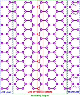
Figure 1: Schematic representation of the Kane-Mele nanoribbon with the honeycomb lattice structure. The ribbon is infinite in the $x$-direction and finite in the $y$-direction with armchair edges. The system is connected to left and right leads. A scattering region at the center hosts vacancy defects arranged on a zigzag chain highlighted by a red rectangle box on the diagram. Armchair chain numbers are labeled by $N$. The vacant sites are denoted by open red circles which are introduced on armchair chains of $N=1,\ 4,\ 7,\ 10$.

II.1 Model Hamiltonian and system geometry

The Kane-Mele model Hamiltonian captures the topological properties of the system, considering the interplay between hopping terms, spin-orbit coupling, and staggered on-site potentials. For a honeycomb lattice ribbon with armchair edges, infinite in the $x$-direction and finite in the $y$-direction, shown in Fig. 1, the tight-binding Hamiltonian is given by Kane01 ; Kane02 :

$$\begin{split}{\cal H}_{KM}&=-t\sum_{\langle m,n\rangle,\sigma}c_{m,\sigma}^{\dagger}c_{n,\sigma}\\ &-i\lambda_{SO}\sum_{\langle\langle m,n\rangle\rangle,\sigma,\sigma^{\prime}}e^{i\nu_{mn}\phi}c_{m,\sigma}^{\dagger}(\bm{\sigma}_{\sigma,\sigma^{\prime}})_{z}c_{n,\sigma^{\prime}}\\ &+M\sum_{m,\sigma}(-1)^{m}c_{m,\sigma}^{\dagger}c_{m,\sigma}\end{split}$$ (1)

Here, $c_{m,\sigma}^{\dagger}~{}(c_{m,\sigma})$ creates (annihilates) an electron at site $i$ with spin $\sigma$, $t$ is the nearest-neighbor hopping amplitude, $\lambda_{SO}$ is the spin-orbit coupling strength, $M$ represents the staggered on-site potential, and $e^{i\nu_{mn}\phi}$ is a phase factor in which $\nu_{mn}=\pm 1$ indicates the direction of the next-nearest-neighbor hopping. The sums are taken over nearest neighbors $\langle m,n\rangle$ and next-nearest neighbors $\langle\langle m,n\rangle\rangle$. ${\bf\sigma}=\sigma_{x}{\bf e}_{x}+\sigma_{y}{\bf e}_{y}$ is the well-known Pauli spin operator. The system is configured as a ribbon attached to left and right leads, forming a scattering region in the center. Figure 1 illustrates the geometry with vacancy defects arranged in a line which is shown by a red rectangle box. Importantly, placing a vacancy defect on a given site is equivalent to turning off the hopping terms that connect this site to its neighbors. These vacancies play a pivotal role in inducing topological Fano resonances, as will be explored in subsequent sections.

II.2 The topological Fano profile 

In the Kane-Mele model, the topological nature of the system manifests in the existence of topologically protected edge states within the energy gap. These edge states, forming helical edge bands, give rise to an edge current that is impervious to backscattering, a hallmark of the topological phase. In the absence of mechanisms facilitating backscattering, the edge current remains unaffected even in the presence of nonmagnetic defects like vacancies. However, the introduction of vacancies in a specific arrangement, forming a conduction channel that connects the upper and lower edges of the ribbon, can lead to the emergence of topological Fano resonance. This channel is effectively created by engineering the defects in a line across the width of the ribbon. It is noteworthy that the presence of vacancy defects, in contrast to on-site impurities with finite potential Rahmati01 , induces discrete energy-bound states around zero energy. Due to the particle-hole symmetry of the system the energy of these bound states will be symmetrically distributed around $E=0$.

Our focus now shifts to the quantum transport through the ribbon in the presence of vacancy defects. In current investigation, the armchair chains are labeled by integer numbers $N=1~{},2,~{}3,~{}\cdots$, and four vacancy defects are introduced on a zigzag chain, situated on armchair chains $N=1,\ 4,\ 7,\ 10$ as illustrated in Fig. 1. We specifically consider a ribbon with a width of $N=10$, indicating the number of armchair chains across the width. The vacancies are regularly arranged so that the distance between two consecutive vacant sites is equal to three zigzag chains. In order to check the accuracy of our analytical simulation of the vacancy-induced topological Fano resenance in the specified structure, which will be detailed in next section, we obtain the transmission spectrum of the system by employing the LB formalism for conduction in confined structures Gamayun01 . For our analysis, we set the hopping amplitude $t=1$ as the unit of energy, and to maintain the system in the topological phase, we choose a fixed spin-orbit coupling of $\lambda_{\text{SO}}=0.2$, while keeping the staggered potential $M=0$ for simplicity. The line of vacancy defects is highlighted by a red rectangle box. Our findings reveal distinctive dips in the transmission spectrum through the ribbon which is shown in Fig. 2. Intriguingly, these dips appear in pairs and exhibit symmetrical distribution in the energy space around $E=0$. It is important to note that upon closer examination of the profile, it is evident that the dips do not exhibit symmetrical behavior with respect to the energies at which they occur. Fano resonance phenomenon often reveals itself through the asymmetrical dips in occurrence energies, a unique fingerprint of this effect. This phenomenon signifies the occurrence of topological Fano resonance in the Kane-Mele model, forming the crux of our study, which we delve into further details in the subsequent sections.

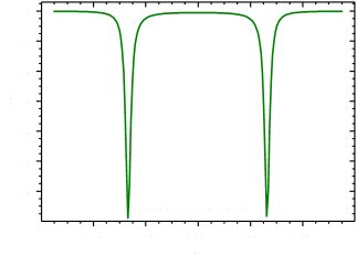
Figure 2: Transmission spectrum through a Kane-Mele nanoribbon of width $N=10$, calculated using the LB formalism for conduction in confined structures. The ribbon is in the topological phase with a fixed hopping amplitude $t=1$ as the energy unit, spin-orbit coupling $\lambda_{\text{SO}}=0.2$, and staggered potential $M=0$. Four vacancy defects are strategically placed in a line on armchair chains $m=1,4,7,10$, forming a conduction channel connecting the upper and lower edges. The transmission spectrum exhibits pairs of dips symmetrically distributed in the energy space around $E=0$, indicative of the topological Fano resonance.

III Transmission analysis 

In the presence of multiple vacancy defects arranged in a line, each defect introduces a discrete energy level within the gap region of the Kane-Mele nanoribbon. These localized states, associated with the vacancies, exhibit localization in real space, forming a spatial pattern that aligns with the arrangement of the defects. Crucially, when defects are strategically placed, the associated states overlap, creating a conduction channel that connects the upper and lower edges of the ribbon. To understand the coupling of these localized states with the edge states and the emergence of the topological Fano resonance, we employ the LS approach. This theoretical framework allows us to obtain an explicit analytical expression for the scattering amplitude of the edge electrons through the presence of multiple vacancy defects. The resulting scattering amplitude reveals a Fano resonance profile in the transmission spectrum, characterized by tunable dips symmetrically distributed around $E=0$. The position and width of these resonances are influenced by the arrangement of the vacancy defects, offering a means to control and engineer the topological Fano resonance in the Kane-Mele nanoribbon.

The combination of the discrete energy levels induced by vacancy defects, their coupling to the edge bands, and the resulting Fano resonance in the transmission spectrum forms the basis for our exploration of vacancy-induced topological Fano resonances in the Kane-Mele nanoribbon. In the subsequent sections, we will provide a detailed analysis of these phenomena, shedding light on the rich interplay between topology, defects, and quantum transport in two-dimensional materials.

III.1 Discrete energy levels associated with a line of vacancy defects 

While the theorem governing the creation of zero energy modes in bipartite lattices due to a single vacancy site is well-established for honeycomb lattices in the absence of spin-orbit coupling $(\lambda_{SO}=0)$ Brouwer01 ; Pereira01 , its applicability to more complex lattice structures, such as the Kane-Mele model, requires further examination.

For graphene, where only nearest-neighbor hopping is considered, the Hamiltonian can be represented in the matrix block form as

$$\Big{(}\begin{array}[]{cc}{\bf 1}&H_{AB}\\ H_{AB}^{\dagger}&{\bf 1}\end{array}\Big{)},$$ (2)

satisfying the conditions for the creation of a localized zero energy mode Pereira01 . Here $A$ and $B$ refers to two sublattices of the bipartite lattice, and $H_{AB}$ and ${\bf 1}$ stand the hopping and identity matrices, respectively. The extension of this result to materials like phosphorene, with next-nearest hopping amplitudes, yields localized states with non-zero energy Amini01 . In our specific case of the Kane-Mele Hamiltonian, ${\cal H}_{KM}$, the direct applicability of Eq. (2) is not immediately evident. However, our numerical simulations demonstrate that even in the presence of spin-orbit coupling ($\lambda_{SO}\neq 0$), a single vacancy defect gives rise to a zero-energy localized state Rahmati01 ; Sadeghizadeh01 ; AlShuwaili01 .

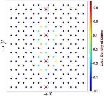
Figure 3: The spatial profile of the local density of states (LDOS) corresponds to the configuration shown in Fig. 1, as it is clearly visible from the figure, the presence of the vacancies creates a conduction channel between the edge states at the upper and lower armchair edges of the ribbon. This channel provides the necessary platform for the occurrence of the backscattering events and the observation of topological Fano resonance in the transmission spectrum of the system. The vacancies are marked with cross symbols. 

To validate the mentioned behavior, the Kane-Mele model for the honeycomb lattice was considered and the local density of states around a single vacancy defect was examined. The obtained results verify the emergence of a localized state with zero energy, affirming the presence of vacancy-induced discrete energy levels Rahmati01 ; Sadeghizadeh01 ; AlShuwaili01 .

It is worth noting that the expressions for the edge states in the presence of spin-orbit interaction Rahmati01 ; Sadeghizadeh01 become notably more intricate compared to the case without it ($\lambda_{\text{SO}}=0$) AlShuwaili01 . Consequently, deriving an exact analytic expression for the localized wave function associated with a single vacancy defect in the presence of spin-orbit coupling ($\lambda_{\text{SO}}\neq 0$) would entail increased complexity, surpassing the scope of this current study. The detailed analysis of such wave functions remains an avenue for future investigations.

Let us now proceed to the scenario of an infinite number of vacancy defects periodically placed in the bulk honeycomb lattice. The resultant band structure of the Kane-Mele model in the presence of spin-orbit interaction has been examined in details by using both the numerical and semi-analytical methods in Refs. Rahmati01 ; Sadeghizadeh01 ; AlShuwaili01 . Using the information reported in these research works, it is possible to examine the periodic arrangement involves placing the vacancy defects such that there are three armchair chains between adjacent defects, essentially mirroring the configuration illustrated in Fig. 1 but extending infinitely in the $y$-direction. For this examination, a non-zero spin-orbit coupling strength of ($\lambda_{SO}\neq 0$) has been considered. The resulting band structure reveals an additional energy band within the original energy gap, attributed to the formation of an impurity band. Each vacancy defect induces a localized wave function akin to a single atomic orbital. These localized wave functions, resembling atomic orbitals, overlap with neighboring wave functions from adjacent vacancy defects, giving rise to the impurity band. Remarkably, the obtained impurity band can be well-described by a simple tight-binding band dispersion, represented as $E(k)=2\Delta\sin(ka)$, where $\Delta$ and $a$ are the band width parameter and the lattice constant, respectively.

The presence of a vacancy defect introduces a discrete energy level at zero with a localized wave function reminiscent of a single-level atom. In the case of a finite number of closely situated vacancy defects, effective overlap occurs between these wave functions, facilitating effective tunneling, $\Delta$, and resulting in finite discrete energy levels symmetrically distributed around zero. These energy levels exhibit extended wave functions across the width of the ribbon, connecting the upper and lower edges and allowing for backscattering. This phenomenon manifests as Fano anti-resoances in the transmission spectrum of the system which will be described in the following.

For a closer examination of the conductive channel created between the edge modes at the upper and lower weirs around the ribbon depicted in Fig. 1, the spatial profile of the local density of states is displayed in Fig. 3. The illustrated profile corresponds to that arrangement of the vacant sites shown in Fig. 1. As can be seen from the figure evidently, the overlap of the zero-energy localized modes around the vacant sites forms a conduction channel between the upper and lower edges of the ribbon. Consequently, the backscattering of the electrons during their passing through this conductive channel, causes the observation of the topological Fano resonance in the considered system.

III.2 Calculation of the Fano anti-resonances using the Lippmann–Schwinger approach 

The purpose of this section is to simulate the topological Fano resonance observed in the transmission spectrum shown in figure 2. To model the quantum transport through the specified system and calculate Fano anti-resonances, the Hamiltonian of

$${\cal H}={\cal H}_{E}+{\cal H}_{V}+{\cal H}_{EV},$$ (3)

is employed in which Hamiltonian ${\cal H}_{E}$ corresponds to the helical edge states of the Kane-Mele model and is expressed as:

$$\begin{split}{\cal H}_{E}&=\int_{-\pi}^{+\pi}\hbar{\rm v}_{F}k_{U}|k_{U}\rangle\langle k_{U}|dk_{U}\\ &\qquad\qquad+\int_{-\pi}^{+\pi}\hbar{\rm v}_{F}k_{L}|k_{L}\rangle\langle k_{L}|dk_{L}.\end{split}$$ (4)

in which it is assumed that at the upper side, the continuum edge state travels to the right with the Fermi speed of ${\rm v}_{F}$, while at the lower side, it is traveling to the left at the same speed. Additionally, the lattice constant, $a$, is assumed to be one. Here, $k_{U}$ and $k_{L}$ represent, respectively, the wave vectors for edge modes at the upper and lower edges associated to the ribbon displayed in Fig. 1. Hereafter, the $U$ and $L$ indices refer to the upper and lower edges.

The Hamiltonian ${\cal H}_{V}$ describes the line of vacancy defects:

$${\cal H}_{V}=E_{0}|v\rangle\langle v|,$$ (5)

describing a quantum dot with energy of $E_{0}$. Here, $|v\rangle$ is the ket-state corresponding to one of the discrete energy states which are induced by the defects. It is assumed that this vacancy state has been coupled with the continuum edge states.

The coupling interaction between the edge states and the defect state is given by ${\cal H}_{EV}$:

$$\begin{split}{\cal H}_{EV}&=\int_{-\pi}^{+\pi}u_{U}(k_{U})|k_{U}\rangle\langle v|dk_{U}\\ &+\int_{-\pi}^{+\pi}u_{L}(k_{L})|k_{L}\rangle\langle v|dk_{L}+H.C.\end{split}$$ (6)

in which $H.C.$ stands for the Hermitian conjugate and the related term ensures the hermiticity of the Hamiltonian. Also, $u_{U}(k_{U})$ and $u_{L}(k_{L})$ represent the coupling strengthes between the discrete vacancy state of $|v\rangle$, and the continuum edge modes of $|k_{U}\rangle$ and $|k_{L}\rangle$ at the upper and lower edges of the considered ribbon, respectively.

The LS formulation of the formal scattering theory can be used to calculate the transmission coefficient. This equation, which is a key concept in quantum mechanics, particularly in the context of scattering, reads

$$|\psi_{out}\rangle=|\psi_{in}\rangle+G_{0}(E)V|\psi_{out}\rangle,$$ (7)

where $|\psi_{in}\rangle$ is the incoming or unperturbed wave state, $|\psi_{out}\rangle$ is the full output or scattered wave function, $E$ is the energy of the specified scattering system, $G_{0}(E)$ is the free-particle Green’s function, and $V$ is the interaction potential.

By defining the transition operator, ${\cal T}(E)$, as

$$V|\psi_{out}\rangle={\cal T}(E)|\psi_{in}\rangle,$$ (8)

the LS equation can be rewritten as follows:

$$|\psi_{out}\rangle=|\psi_{in}\rangle+G_{0}(E){\cal T}(E)|\psi_{in}\rangle.$$ (9)

By multiplying both sides of the above equation by $V$, it can be converted into an equation to find the transition operator, ${\cal T}(E)$, as:

$${\cal T}(E)=V+VG_{0}(E){\cal T}(E).$$ (10)

Usually, using the iteration method, the solution of the transition operator can be written as an infinite expansion of the Green’s operator $G_{0}(E)$ and the interaction potential $V$ as

$${\cal T}(E)=V+VG_{0}(E)V+VG_{0}(E)VG_{0}(E)V+\cdots.$$ (11)

In the considered problem, the interaction potential $V$ is equivalent to the term of ${\cal H}_{EV}$ in the entire Hamiltonian and the Green operator, $G_{0}(E)$, is the associated to the rest of the Hamiltonian, ${\cal H}_{E}+{\cal H}_{V}$. Consequently, it is possible to write:

$$G_{0}(E)=G_{E}(E)+G_{V}(E),$$ (12)

in which

$$\begin{split}G_{E}(E)=&\int_{-\pi}^{+\pi}{|k_{U}\rangle\langle k_{U}|\over E-\hbar{\rm v}_{F}k_{U}+i0^{+}}dk_{U}\\ &\qquad\qquad+\int_{-\pi}^{+\pi}{|k_{L}\rangle\langle k_{L}|\over E+\hbar{\rm v}_{F}k_{L}+i0^{+}}dk_{L},\end{split}$$ (13)

and

$$G_{V}={|v\rangle\langle v|\over E-E_{0}+i0^{+}}.$$ (14)

After some algebraic operation, it can be shown that

$$VG_{0}(E)VG_{0}(E)V=\alpha V,$$ (15)

where $\alpha$ is given by the expression of

$$\begin{split}\alpha&=g_{0}(E)\Big{(}\int_{-\pi}^{+\pi}{\big{|}u_{U}(k_{U})\big{|}^{2}\over E-\hbar{\rm v}_{F}k_{U}+i0^{+}}dk_{U}\\ &\qquad\qquad+\int_{-\pi}^{+\pi}{\big{|}u_{L}(k_{L})\big{|}^{2}\over E+\hbar{\rm v}_{F}k_{L}+i0^{+}}dk_{L}\Big{)},\end{split}$$ (16)

in which

$$g_{0}(E)={1\over E-E_{0}+i0^{+}}.$$ (17)

The combination of Eqs. (10) and (15) leads to

$${\cal T}(E)={V+VG_{0}(E)V\over 1-\alpha}.$$ (18)

In the following calculation, it is assumed that the interaction occurring during the scattering process is both short-range and local. Also, for simplicity, it is assumed that $u_{U}(k_{U})$ and $u_{L}(k_{L})$ are some constant functions denoted by $u_{U}$ and $u_{L}$, respectively. If the interaction that leads to scattering is completely local, this is an accurate assumption. But, since in the specified system this interaction is not completely local, this assumption is an approximation in our study. Of course, in the following by comparing the simulation results with those obtained from LB formulation, we will see that this approximation is very good and efficient. Anyway, this assumption helps us to easily calculate the integrals appearing in Eqs. (16), so that we have:

$$\begin{split}\int_{-\pi}^{+\pi}{1\over E-\hbar{\rm v}_{F}k_{U}+i0^{+}}dk_{U}={i\pi\over\hbar{\rm v}_{F}},\\ \int_{-\pi}^{+\pi}{1\over E+\hbar{\rm v}_{F}k_{L}+i0^{+}}dk_{L}={i\pi\over\hbar{\rm v}_{F}}.\end{split}$$ (19)

With the above results, $\alpha$ is reduced to:

$$\alpha=\alpha_{U}+\alpha_{L},$$ (20)

where

$$\begin{split}\alpha_{U}&=g_{0}(E)\Big{(}{\pi i\over\hbar{\rm v}_{F}}\Big{)}\big{|}u_{U}\big{|}^{2},\\ \alpha_{L}&=g_{0}(E)\Big{(}{\pi i\over\hbar{\rm v}_{F}}\Big{)}\big{|}u_{L}\big{|}^{2}.\end{split}$$ (21)

To obtain the transmission coefficient, an initial edge state is considered which travels along the upper edge of the ribbon with an initial momentum of $k_{0}$. Consequently, at a far distance before the defect, the initial state can be represented as;

$$\langle\ell|\psi_{in}\rangle=\langle\ell|k_{0}\rangle=e^{ik_{0}\ell}.$$ (22)

Here, the lattice constant is assumed as the unit of length and $\ell\to-\infty$. To know the transmission probability, we should calculate the probability of detecting the particle at a far distance after the central scattering region and along the upper side of the ribbon. If the particle is detected in this distance, it means that the output wave function can be displayed as

$$\langle\ell|\psi_{out}\rangle=t\langle\ell|k_{0}\rangle=te^{ik_{0}\ell},$$ (23)

in which $t$ is the transmission amplitude and $\ell\to+\infty$. Multiplying both sides of Eq.(9) by bra-basis of $\langle\ell|$ reads:

$$\langle\ell|\psi_{out}\rangle=\langle\ell|\psi_{in}\rangle+\langle\ell|G_{0}(E){\cal T}(E)|\psi_{in}\rangle.$$ (24)

Using the fact that for the considered case

$$V=\int_{-\pi}^{+\pi}u_{U}(k_{U})|k_{U}\rangle\langle v|dk_{U}+H.C.,$$ (25)

and

$$G_{0}(E)=\int_{-\pi}^{+\pi}{|k_{U}\rangle\langle k_{U}|\over E-E_{0}+i0^{+}}dk_{U},$$ (26)

it can be shown that

$$\begin{split}\langle\ell|G_{0}(E){\cal T}(E)|k_{0}\rangle=&{g_{0}(E)\over 1-\alpha}\\ \times\int_{-\pi}^{+\pi}&{u_{U}^{*}(k_{U})u_{U}(k_{0})e^{ik_{0}\ell}\over E-i{\rm v}_{F}k_{U}+i0^{+}}dk_{U}.\end{split}$$ (27)

Considering that $u_{U}(k_{U})$ and $u_{U}(k_{0})$ can be assumed equal to a constant value of $u_{U}$, the following closed form expression can be derived

$$\langle\ell|G_{0}(E){\cal T}(E)|k_{0}\rangle={2\alpha_{U}\over 1-\alpha}e^{ik_{0}\ell},$$ (28)

Finally, by inserting Eqs. (22), (23), and (28) in Eq. (24), and performing some algebraic calculation, the transmission amplitude is drivable as

$$t=1+{2\alpha_{U}\over 1-\alpha}={1+\alpha_{U}-\alpha_{L}\over 1-\alpha_{U}-\alpha_{L}}.$$ (29)

If the coupling between the discrete vacancy and the continuous upper-edge states is absent, we have $u_{U}=0$ and consequently $\alpha_{U}=0$. Then, as expected and is clear from the above equation, $t=1$ which result in a perfect transmission. On the other hand, if there is no coupling between the discrete vacancy and the continuous lower-edge states, then $u_{L}=0$ and $t$ is reduces to

$$t={1+\alpha_{U}\over 1-\alpha_{U}}.$$ (30)

Since $\alpha_{U}$ is purely imaginary, $T(E)=|t|^{2}=1$ and the transmission is complete, as is expected. But in the interaction with the lower edge, there is a possibility of reflection and scattering to the lower wire. This discussion confirms that for observing the topological Fano resonance in a Kane-Mele nanoribbon, it is essential that the vacancy discrete states becomes coupled with the continuous edge modes on both upper and lower sides. Also, the above fact indicates that the strength of coupling between discrete and continuous modes affects the quality of observing Fano resonance.

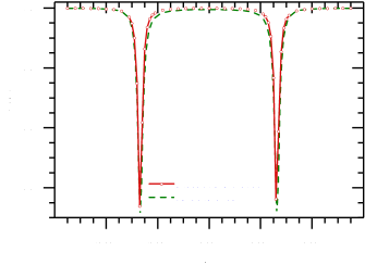
Figure 4: Comparison of the transmission spectrum of the specified system obtained from the current simulation based on the LS scattering formalism and the results obtained from LB formulation. This comparison verifies the efficiency and accuracy of the simulation method presented in this study confirming the occurence of the topological Fano resonance in the considered structur. 

In Fig. 4, the analytically simulated transmission probability, $T(E)$, is plotted as a function of energy, $E$, and is compared with the calculations obtained from LB formalism. As expected, the two graphs are both qualitatively and quantitatively very similar and this figure correctly shows the behavior exhibited in Fig. 2. The very good match of the two graphs shows that the assumption that $u_{U}(k_{U})$ and $u_{L}(k_{L})$ are constant is an approximation that is very close to being accurate. This figure shows that despite the simplicity of the carried simulation based on LS scattering formulation, it is reasonably efficient and accurate in quantitative and qualitative prediction of the topological Fano resonance in Kane-Mele nanoribbons.

IV Summary and Conclusion 

A nanoribbon of a two-dimensional hexagonal lattice with finite width and armchair edges, which governed by the Kane-Mele Hamiltonian, was considered. This Hamiltonian describes the spin-orbit interaction which leads to the quantum spin Hall effect. It was assumed that the length of the ribbon at the far distances is limited to two left and right leads. As a result, at the armchair sides, edge continuum states, which are topologically protected, flowed to the left and right with Fermi velocities. It was assumed that the length of the ribbon, at long distances, was limited to two left and right leads. As a result, at the armchair sides, edge continuum states, which are topologically protected, traveled to the left and right with Fermi velocities. This situation was similar to considering the ribbon’s sides as two current-carrying wires. By creating a regular array of on-site vacancies on a zigzag chain across the width of the ribbon, a conduction channel between the edge wires of the ribbon was created. This cannel caused the creation of a central scattering region around the zigzag chain that contained the vacancy defects. Also, this conduction channel, which is due to the overlap of zero-energy localized states surrounding the vacant sites, allows the creation of discrete vacancy states, the coupling of these discrete states with continuous edge states, and the occurrence of backscattering events. It saw shown that the coupling of topologically protected continuous edge states and the discrete vacancy states and their interference with each other made it possible to observe topological Fano resonance. First, the Fano topological resonance profile was produced using the LB formulation. Then, employing the LS scattering formalism and using the Green’s operator as well as the transition matrix this profile was simulated, analytically. In the calculations, it was shown that the transmission spectrum of the desired system is a function of the energy of the system and the degree of coupling between the discrete vacant states with the continuous edge states on both sides of the ribbon. By adjusting the width of the ribbon, choosing the number of vacancies, and checking how they are arranged on the zigzag chain across the ribbon, it is possible to adjust and control the vacancy-induced topological Fano resonance in the Kane-Mele nanoribbons. From an analytical perspective, the simulation of topological Fano resonance involves using the LS scattering framework. This research provides a benefit by performing associated calculations analytically, producing outcomes that closely match those obtained using the LB approach, showcasing both quantitative and qualitative precision. These findings contribute to the understanding of the impact of vacancies on the electronic and transport properties of nanoribbons, which is essential for the design, control, and sensing applications of such systems.

- (1) U. Fano, Phys. Rev. 124, 1866 (1961).
- (2) A. E. Miroshnichenko, S. Flach, and Y. S. Kivshar, Rev. Mod. Phys. 82, 2257 (2010).
- (3) O. Újsághy, J. Kroha, L. Szunyogh, and A. Zawadowski, Phys. Rev. Lett. 85, 2557 (2000).
- (4) A. C. Johnson, C. M. Marcus, M. P. Hanson, and A. C. Gossard, Phys. Rev. Lett. 93, 106803 (2004).
- (5) K. Kobayashi, H. Aikawa, S. Katsumoto, and Y. Iye, Phys. Rev. Lett. 88, 256806 (2002).
- (6) E. O. Kamenetskii, G. Vaisman, and R. Shavit, J. Appl. Phys. 114, 173902 (2013).
- (7) A. Attaran, S. D. Emami, M. R. K. Soltanian, R. Penny, F. behbahani, S. W. Harun, H. Ahmad, H. A. Abdul-Rashid, and M. Moghavvemi, Plasmonics 9, 1303 (2014).
- (8) B. Lv, R. Li, J. Fu, Q. Wu, K. Zhang, W. Chen, Z. Wang, and R. Ma, Sci. Rep. 6, 31884 (2016).
- (9) J. Gores, D. Goldhaber-Gordon, S. Heemeyer, M. A. Kastner, H. Shtrikman, D. Mahalu, and U. Meriav, Phys. Rev. B 62, 2188 (2000).
- (10) S. Bandopadhyay, B. Dutta-Roy, and H. S. Mani, Am. J. Phys. 72, 15011507 (2004)
- (11) S. Stassi, A. Chiadó, G. Calafiore, G. Palmara, S. Cabrini, and C. Ricciardi, Sci. Rep. 7, 1065 (2017)
- (12) A. Overviga, and A. Alú, Adv. Photonics 3, 026002-1 (2021)
- (13) B. Lukýanchuk, N. I. Zheludev, S. A. Maier, N. J. Halas, P. Nordlander, H. Giessen, and C. T. Chong, Nat. Mater. 9, 707715 (2010)
- (14) P. S. Deo, and C. Basu, Phys. Rev. B 52, 10685(1995).
- (15) A. E. Miroshnichenko, and Y. S. Kivshar, Phys. Rev. E 72, 056611(2005).
- (16) A. Chakrabarti, Phys. Lett. A 366, 507 (2007).
- (17) M. E. Torio, K. Hallberg, A. H. Ceccatto, and C. R. Proetto, Phys. Rev. B 65, 085302 (2002).
- (18) A. Rodriguez, F. Dominguez-Adame, I. Gomez, and P.A. Orellana, Phys. Lett. A 320, 242 (2003).
- (19) M. L. Ladron de Guevara, F. Claro, and P. A. Orellana, Phys. Rev. B 67, 195335 (2003).
- (20) M. Amini, M. Soltani, and M. Sharbafiun, Phys. Rev. B 99, 085403 (2019).
- (21) M. Amini, M. Soltani, S. Baninajarian, and M. Rezaei, Phys. Lett. A 387, 127012 (2021).
- (22) M. Z. Hasan and C. L. Kane, Rev. Mod. Phys. 82, 3045 (2010).
- (23) F. Zangeneh-Nejad and R. Fleury, Phys. Rev. Lett. 122, 014301 (2019).
- (24) C. Y. Ji, Y. Zhang, B. Zou, and Y. Yao, Phys. Rev. A. 103, 023512 (2021).
- (25) W. Wang, Y. Jin, W. Wang, B. Bonello, B. Djafari-Rouhani, and R. Fleury, Phys. Rev. B 101, 024101 (2020).
- (26) C. Sun, A. Song, Z. Liu, Y. Xiang, and F. Z. Xuan, AIP Advances 13, 025008 (2023).
- (27) C. L. Kane, and E. J. Mele, Phys. Rev. Lett. 95, 146802 (2005).
- (28) C. L. Kane and E. J. Mele, Phys. Rev. Lett. 95, 226801 (2005).
- (29) F. Rahmati, M. Amini, M. Soltani, and M. Sadeghizadeh, Phys. Rev. B 107, 205408 (2023).
- (30) O. Gamayun, Y. Zhuravlev, and N. Iorgov, J. Phys. A Math. Theor. 56, 205203 (2023)
- (31) P. W. Brouwer, E. Racine, A. Furusaki, Y. Hatsugai, Y. Morita, and C. Mudry, Phys. Rev. B 66, 014204 (2002).
- (32) V. M. Pereira, J. M. B. Lopes dos Santos, and A. H. Castro Neto, Phys. Rev. B 77, 115109 (2008).
- (33) M. Sadeghizadeh, M. Soltani, and M. Amini, Sci. Rep. 13, 12844 (2023).
- (34) H. Al-Shuwaili, Z. Noorinejad, M. Amini, M. Soltani, E. Ghanbari-Adivi, Submitted to be published (2024)