DualView: Data Attribution from the Dual Perspective

Galip Ümit Yolcu¹ Thomas Wiegand^1,2,3 Wojciech Samek^1,2,3,† Sebastian Lapuschkin^1,†

( ¹ Fraunhofer Heinrich-Hertz-Institute, 10587 Berlin, Germany
² Technische Universität Berlin, 10587 Berlin, Germany
³ BIFOLD – Berlin Institute for the Foundations of Learning and Data, 10587 Berlin, Germany
^† corresponding authors: {wojciech.samek,sebastian.lapuschkin}@hhi.fraunhofer.de )

Abstract

Local data attribution (or influence estimation) techniques aim at estimating the impact that individual data points seen during training have on particular predictions of an already trained Machine Learning model during test time. Previous methods either do not perform well consistently across different evaluation criteria from literature, are characterized by a high computational demand, or suffer from both. In this work we present DualView, a novel method for post-hoc data attribution based on surrogate modelling, demonstrating both high computational efficiency, as well as good evaluation results. With a focus on neural networks, we evaluate our proposed technique using suitable quantitative evaluation strategies from the literature against related principal local data attribution methods. We find that DualView requires considerably lower computational resources than other methods, while demonstrating comparable performance to competing approaches across evaluation metrics. Futhermore, our proposed method produces sparse explanations, where sparseness can be tuned via a hyperparameter. Finally, we showcase that with DualView, we can now render explanations from local data attributions compatible with established local feature attribution methods: For each prediction on (test) data points explained in terms of impactful samples from the training set, we are able to compute and visualize how the prediction on (test) sample relates to each influential training sample in terms of features recognized and by the model. We provide an Open Source implementation of DualView online¹¹1https://github.com/gumityolcu/DualView_Data_Attribution_Influence_Estimation, together with implementations for all other local data attribution methods we compare against, as well as the metrics reported here, for full reproducibility.

1 Introduction

Deep Neural Networks (DNN) are being employed on critical decision making processes with considerable impacts on human lives Hu et al., (2018); Hayashi, (2022). The opaque nature of these complex models often makes their application problematic in high-stakes scenarios Tolan et al., (2019). As a consequence, the Machine Learning (ML) community has developed solutions to dissect and understand the inference processes employed by complex predictors under the area of Explainable Artificial Intelligence (XAI). A majority of work in XAI is focused on feature attribution; the attribution of scores to input (or hidden) features which indicating their importance for the prediction being explained. Local data attribution on the other hand concerns itself with the problem of determining the training data points that are responsible for a particular prediction of a trained model on a specific test input. Local data attribution is also been referred to as ”influence estimation” Hammoudeh and Lowd, (2023), with reference to the seminal work of Koh and Liang, (2017) which uses Influence Functions to explain neural network decisions.

Currently, there are several key approaches to local data attribution: Similarity metrics measure how similar the test point is to each training point from the perspective of the machine learning model Charpiat et al., (2019); Hanawa et al., (2021); Engel et al., (2023). Approaches based on Influence Functions estimate the effect of discarding (individual) training points and then retraining the model Koh and Liang, (2017); Barshan et al., (2020) Other approaches build on the decomposition of the model output after inference into the contributions of each training point Yeh et al., (2018) or the tracking of effects of training points throughout training Chen et al., (2021); Pruthi et al., (2020).

In general, the evaluation of explanations of DNN decisions is a challenging task, in particular due to the absence of ground truth knowledge about the expected explanation. In the area of local feature attribution, numerous XAI evaluation metrics have been proposed throughout the last decade, which aim at measuring different desirable properties of explanations (e.g. faithfulness to model behaviour Samek et al., (2017), robustness Yeh et al., (2019), dependency on model parameters Adebayo et al., (2018)). Similarly, in the area of local data attribution, several (yet by far not as many as for feature attribution) evaluation methods have been proposed from with matching intent Han et al., (2020); Hanawa et al., (2021); Pezeshkpour et al., (2021).

In general, the concept of quantitative evaluation of explanation methods is not yet as rigorously implemented in the area of local data attribution, as it is the case in the area of local feature attribution Hedström et al., (2023). While Hanawa et al., (2021), for example, evaluates several data attribution methods in terms of how well they reflect similarity of input data points, the work does not draw in other aspects of data attribution methods which have been widely utilized for evaluation purposes in the literature, e.g. how helpful they are to clean datasets Koh and Liang, (2017); Yeh et al., (2018); Pruthi et al., (2020) or for detecting mismatches between test and training data distributions Koh and Liang, (2017).

In this work, we contribute as follows. (i) We propose a novel local data attribution method based on the decomposition of the model output, and (ii) present an analysis of the effects of various hyperparameter ranges for this method. (iii) We formulate two evaluation metrics, building on ideas from the literature, which measure the effectiveness of explanations in cleaning datasets with poisoned labels, or in detecting Clever Hans predictions Lapuschkin et al., (2019). (iv) We then evaluate our proposal against prominent methods from literature using these evaluation metrics, along with the metrics from Hanawa et al., (2021) that measure the quality of explanation methods as similarity metrics. Finally, (v) we propose to combine our decomposition-based local data attribution approach with approaches from local feature attribution, providing explanations highlighting not only influential training samples affecting the inference for a given test point, but for the first time also the features on the given test and training instances responsible for the samples’ impact.

2 Notation

Before summarizing the related work and presenting our method proposal, we would like to clarify some notation. Given a training dataset ${\mathcal{D}=\Bigl{\{}(\mathbf{x}_{i},y_{i}),i\in\bigl{[}N\bigr{]}\Bigr{\}}}$ , of $N$ datapoints, where $\mathbf{x}_{i}\in\mathbb{R}^{d}$ are the training data points, ${y_{i}\in\bigl{[}C\bigr{]}}$ are the corresponding classes; we consider a trained DNN which implements the function ${\Phi(~{}\cdot~{};\mathbf{\theta}):\mathbb{R}^{d}\rightarrow\mathbb{R}^{C}}$ that classifies inputs into one of $C$ classes. The DNN is assumed to be trained using gradient descent with the empirical risk:

\mathbf{L}(\mathbf{\theta},\mathcal{D})=\frac{1}{N}\sum_{i=1}^{N}\ell(\Phi(\mathbf{x}_{i};\mathbf{\theta}),y_{i})

where $\ell(\cdot,\cdot)$ is a sample-wise classification loss function, such as the cross entropy loss. We assume the model is composed of a nonlinear feature extractor part ${\mathbf{f}(~{}\cdot~{};\mathbf{\vartheta}):\mathbb{R}^{d}\rightarrow\mathbb{R}^{p}}$ and a final fully connected layer with parameter matrix $W\in\mathbb{R}^{p\times C}$ , with columns $w_{i}\in\mathbb{R}^{p}$ such that $\Phi(\mathbf{x};\mathbf{\theta})=\Phi(\mathbf{x};\mathbf{\vartheta},W)=W^{\top}\mathbf{f}(\mathbf{x};\mathbf{\vartheta})$ . In all cases, we are explaining the output logit corresponding to a specific class $c\in[C]$ . This is essentially asking “Why does the DNN think this input $\mathbf{x}$ might be of class $c$ ?”. In practice, $c$ can be the original (correct) class of the test point, or the decision class of the network $\operatorname*{arg\,max}_{c}\Phi(\mathbf{x};\mathbf{\theta})_{c}$ . These two options agree for correctly classified test points. We want methods to determine the attributions $A_{i,c}(\mathbf{x})$ , indicating the relevance of $i^{\text{th}}$ training data point $(\mathbf{x}_{i},y_{i})\in\mathcal{D}$ for the decision of the model on the test point $\mathbf{x}$ .

3 Related Work

Data attribution is part of instance based explanations, along with different approaches: Data summarization and prototype selection methods try to give a succinct representation of the dataset distribution Brophy, (2020). Methods to find criticisms that summarize what is missing from the selected prototypes has also been proposed Bien and Tibshirani, (2011). Data valuation is the problem of determining the effect data points have on the performance of a certain learning algorithm. It constitutes a global explanation both in terms of inputs (by describing the general behaviour of models, not focusing on a particular test point) and model (by considering the interaction between the dataset and the learning algorithm, including the model class, not focusing on a specific, trained model). Similar to data valuation, some recent methods provide explanations that are local in the input sense, but global in the model sense Ilyas et al., (2022); Park et al., (2023). These methods focus on the outcome of the learning algorithm, on a given test input, as the given learning algorithm is applied to different subsets of the training dataset. They require explanation times in the order of tens of minutes, so they are also practically challenging to use Park et al., (2023).

In this paper, we focus on post-hoc local data attribution, estimating the influence of training datapoints on the behaviour of a particular model that is already trained, given a singular test sample.

In the remaining part of this section we review three post-hoc data attribution methods that have been proposed in the literature.

Influence Functions (IF) is a method from robust statistics, which was initially used for the analysis of linear models, in particular for studying the effects of outliers Srikantan, (1961); Hammoudeh and Lowd, (2023). Koh and Liang, (2017) proposed using this method for local data attribution of DNN models. It approximates the effect of discarding a training point and retraining has on the model behaviour on an observed test point. However, this approximation is conditioned on the current trained parameters of the network, and hence includes information about the decision making strategies employed by the trained model which it is explaining. Data attribution by IF is given by

A^{\text{IF}}_{i,c}(\mathbf{x})=\nabla_{\mathbf{\theta}}\ell(\Phi(\mathbf{x};\mathbf{\theta}),c)^{\top}H^{-1}_{\mathbf{\theta}}\nabla_{\mathbf{\theta}}\ell(\Phi(\mathbf{x}_{i};\mathbf{\theta}),y_{i})

(1)

where $H_{\mathbf{\theta}}=\nabla^{2}\mathbf{L}(\mathbf{\theta},\mathcal{D})$ is the Hessian of the loss.

Computation of the inverse Hessian is problematic for modern architectures with millions of parameters. For this reason, Koh and Liang, (2017) propose using the method of Agarwal et al., (2017) to approximate $\ell(\Phi(\mathbf{x}_{\text{test}};\mathbf{\theta}),c)^{\top}H^{-1}_{\mathbf{\theta}}$ for each test point. While this mitigates the computational cost, it does not entirely solve the problem: computing explanations for a single test point can still take a long time, possibly in the order of hours Hammoudeh and Lowd, (2023).

As the Representer Point Selection (RPS) method, Yeh et al., (2018) propose training the final (fully connected) layer until convergence with weight decay regularization. Then, they show that the columns of $W$ can be written as a linear combination of final hidden features of training data points. This means that we can decompose any output $c$ of the new model to the contributions of each training datapoint, yielding:

A^{\text{RPS}}_{i,c}(\mathbf{x})=-\frac{\partial\ell(\Phi(\mathbf{x}_{i};\mathbf{\theta}),c)}{\partial\Phi(\mathbf{x}_{i};\mathbf{\theta})_{c}}\mathbf{f}(\mathbf{x}_{i})^{\top}\mathbf{f}(\mathbf{x})

(2)

Charpiat et al., (2019) propose looking at how much a training step in the gradient direction for one sample changes the output for another sample, as a measure of “Similarity from the Neural Network’s Perspective” (SIM). Since we consider explanations of a certain output logit, we formulate a data attribution method using the same idea: the change in the model output of output logit $c$ on a test point $\mathbf{x}$ , after taking a step in the direction of the gradient of the output logit $y_{i}$ at the training point $\mathbf{x}_{i}$ . With a first order approximation, this yields:

A^{\text{SIM}}_{i,c}(\mathbf{x})=\frac{\nabla_{\mathbf{\theta}}\Phi(\mathbf{x};\mathbf{\theta})_{c}^{\top}\nabla_{\mathbf{\theta}}\Phi(\mathbf{x}_{i};\mathbf{\theta})_{y_{i}}}{\lVert\nabla_{\mathbf{\theta}}\Phi(\mathbf{x}_{i};\mathbf{\theta})_{y_{i}}\lVert_{2}}

(3)

4 Dual Approach to Data Attribution

4.1 Multiclass SVM Surrogate

It is common practice in XAI research to train a surrogate model which is interpretable, to explain opaque ML models Ribeiro et al., (2016); Karim et al., (2022); Mehdi and Tiwary, (2023). There are several model classes that are inherently interpretable in the data attribution sense (e.g. decision trees, kNN classifiers, Support Vector Machines (SVM)). Theoretical work on the implicit bias of gradient descent reveals its margin maximizing behaviour Soudry et al., (2018); Ji and Telgarsky, (2018); Gunasekar et al., (2018); Gidel et al., (2019); Tarzanagh et al., (2023). In particular, Lyu and Li, (2019) prove that with cross-entropy loss, homogeneous models converge to the solution of the following optimization problem under certain conditions (including seperability):

\begin{array}[]{llllll}\min_{W}&\lx@intercol\frac{1}{2}||W||^{2}_{2}\hfil\lx@intercol\\ \textrm{s.t.}&\forall i\in[N],\forall j\in[C]\backslash y_{i}\\ &(w_{y_{i}}^{\top}\mathbf{f}(\mathbf{x}_{i});\mathbf{\vartheta})-(w_{j}^{\top}\mathbf{f}(\mathbf{x}_{i};\mathbf{\vartheta}))\geq 1\\ \end{array}

(4)

This multi-class extension of SVMs differs from separately training multiple SVMs, as is commonly done for multi-class classification, since information from different classification heads is shared through the constraints. The margin maximizing bias of gradient descent is also observed experimentally with non-homogeneous architectures in practical settings Ji and Telgarsky, (2020); Haim et al., (2022), and therefore constitutes a promising direction in surrogate modeling for data attribution of models trained using gradient descent.

4.2 DualView

Similar to Yeh et al., (2018), we propose retraining the final fully connected layer of the DNN. To allow for non-seperable datasets, we solve the extension to the above quadratic programming problem, given by Crammer and Singer, (2001):

\begin{array}[]{llllll}\min_{W}&\lx@intercol\frac{1}{2}||W||^{2}_{2}+K\sum_{i=1}^{N}\xi_{i}\hfil\lx@intercol\\ \textrm{s.t.}&\forall i\in[N],\forall j\in[C]\\ &(w_{y_{i}}^{\top}\mathbf{x}_{i})-(w_{j}^{\top}\mathbf{x}_{i})+\delta_{jy_{i}}\geq 1-\xi_{i}\\ \end{array}

(5)

After solving the dual problem and obtaining the dual variables $\lambda_{ij}\geq 0,\forall i\in[N],\forall j\in[C]$ , we define DualView (DV), with data attribution for the decision of class $c$ as

A^{\text{DV}}_{c,i}(\mathbf{x})=\left\{\begin{array}[]{ll}\sum_{j\neq c}\lambda_{ij}\mathbf{f}(\mathbf{x}_{i};\mathbf{\vartheta})^{\top}\mathbf{f}(\mathbf{x};\mathbf{\vartheta})&\mbox{if }y_{i}=c\\ -\lambda_{ic}\mathbf{f}(\mathbf{x}_{i};\mathbf{\vartheta})^{\top}\mathbf{f}(\mathbf{x};\mathbf{\vartheta})&\mbox{else}\end{array}\right.

(6)

We refer the reader to Appendix A for a derivation and explanation.

DualView is similar in spirit to RP Yeh et al., (2018) in that both methods replace the final layer of the DNN with an interpretable kernel surrogate, using the final hidden features as the kernel. The decomposition of the surrogate weights into the contributions of training datapoints constitutes a global explanation of the model behaviour: following the terminology of Yeh et al., (2018), datapoints with a positive coefficient are excitatory, meaning that being similar to these datapoints is considered as evidence for the class being explained. In contrast, datapoints with negative coefficients have inhibitory effect.

One point of interest in data attribution is the complexity of the explanations. With big datasets of millions of images, methods that result in comparable attributions on too many data points are hard to interpret Iwata and Yoshikawa, (2021). Our choice of surrogate produces sparse explanations by design: only the datapoints that are in the margin obtain nonzero attributions. However, extreme sparsity may hurt the expressivity of the explanations: too few training examples might struggle to capture all aspects of model behaviour. The hyperparameter $K$ allows us to tune the sparsity of explanations by controlling the softness of the margin. We investigate this aspect in further detail in Appendix B.

5 Experimental Evaluation

5.1 Evaluation Metrics

5.1.1 Identical Class Test

Hanawa et al., (2021) propose using a basic test as a minimal requirement that similarity metrics should satisfy: the maximally attributed data point from the training dataset should be of the same class as the decision being explained. We compute the ratio of data points that pass this test. A random attributor that assigns a random and independent value to all training data would have an expected score of $\frac{1}{C}$ for this metric, assuming no class imbalance.

5.1.2 Identical Subclass Test

A further idea introduced by Hanawa et al., (2021) is to group classes of the training dataset into superclasses. The DNN is then trained on this new dataset, and is assumed to learn how to disambiguate the different subclasses inside each superclass. The superclasses are composed of randomly selected subclasses, such that there is no semantic similarity or correlation between the subclasses. Because of this, we expect a data attribution method to indicate the most relevant training data point to be of the same original (sub)class as the test sample. Again, we compute the ratio of test samples that pass this test. A random attributor would also obtain an expected score of $\frac{1}{C}$ for this metric, assuming no class imbalance.

5.1.3 Label Poisoning Experiment

Following Koh and Liang, (2017); Yeh et al., (2018); Pruthi et al., (2020), we randomly change the labels of a subset of training data. Afterwards, we produce a list of relevant samples, sorted in descending order of relevance for all the decisions on the test dataset, not only for a particular test input. While each author has proposed a different ranking strategy for their method, we sort the input data in terms of their cumulative absolute relevances over our test data, in order to have a uniform evaluation strategy.

Afterwards, we consecutively iterate through this list, recording the ratio of the mislabeled samples we detect. This produces a cumulative density curve: for each percentage of training points it shows the amount of poisoned labels found up to the corresponding position in the given ranking. Supposing that a better explainer produces higher attributions to mislabeled datapoints, previous works have investigated how fast this curve increases. We use the area under this curve to formulate a concrete quantification strategy. The maximum possible area for an attributor depends on the number of samples with corrupted labels, and is always less than $1$ . Moreover, the minimum score for the worst performing attributor for this metric is greater than $0$ . We therefore normalize the area under the curve by subtracting the minimum value, and normalizing by the range of possible values. As such, the metric is normalized between $0.$ and $1.$ , and the expected score of a random attributor is $0.5$ .

5.1.4 Domain Mismatch Detection Test

Koh and Liang, (2017) propose changing the training data distribution by hand to introduce a domain mismatch. While they only give a case-specific example, we formulate the idea as a concrete evaluation metric. We will apply a constant perturbation to a subset of the training data points of a single class $j$ . Let $\omega(\cdot)$ be a function that applies a predefined perturbation on its input. Let $\mathcal{D}^{\prime}$ denote the perturbed training dataset where a subset of the data $(\mathbf{x}_{i},j)$ has been replaced with $(\omega(\mathbf{x}_{i}),j)$ . This introduces a dependence between the constant perturbation $\omega(\cdot)$ and the class $j$ . After training a DNN on $\mathcal{D}^{\prime}$ , we discard the test samples of class $j$ and we perturb all other test data points. Out of these test points, we use those which have been classified to class $j$ , indicating that the model is using the artificial connection between the perturbation and the class $j$ . Notice that this results in a reduced number of candidate test points, and a model which is robust to the perturbation being used is going to limit the number of candidate test points more. In such a case, we expect a reasonable explanation method to assign the most relevance to one of the input data points that have been perturbed, indicating that the explanations capture the model behaviour. We compute the ratio of test data points that pass this test.

The expected score for a random attributor is determined by the ratio of the number of marked samples to the total size of the training dataset. This number is $0.030$ for both our experiments.

5.2 Datasets and Models

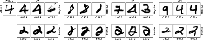
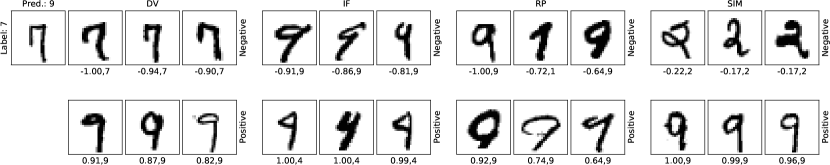
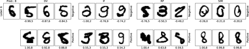
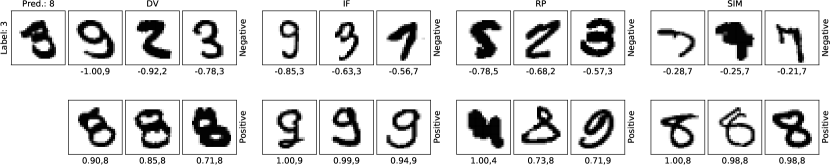
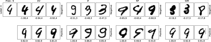
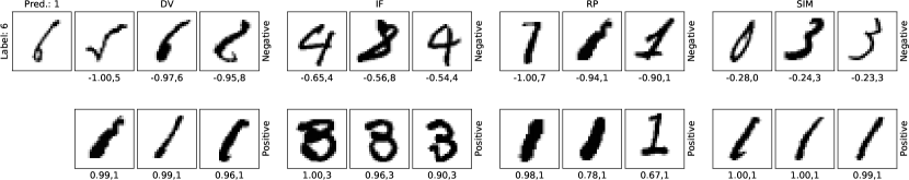
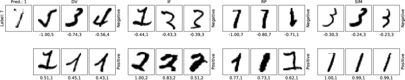
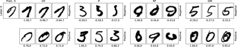
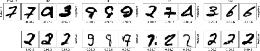
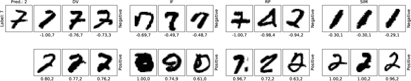
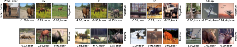
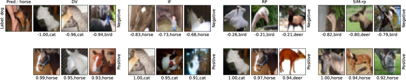
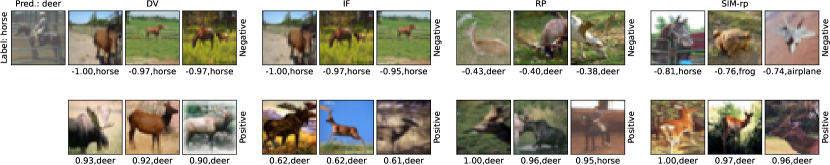
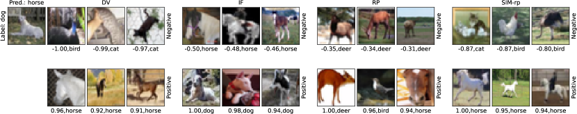
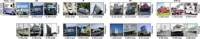
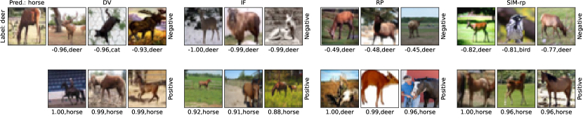
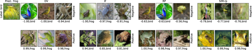
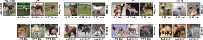
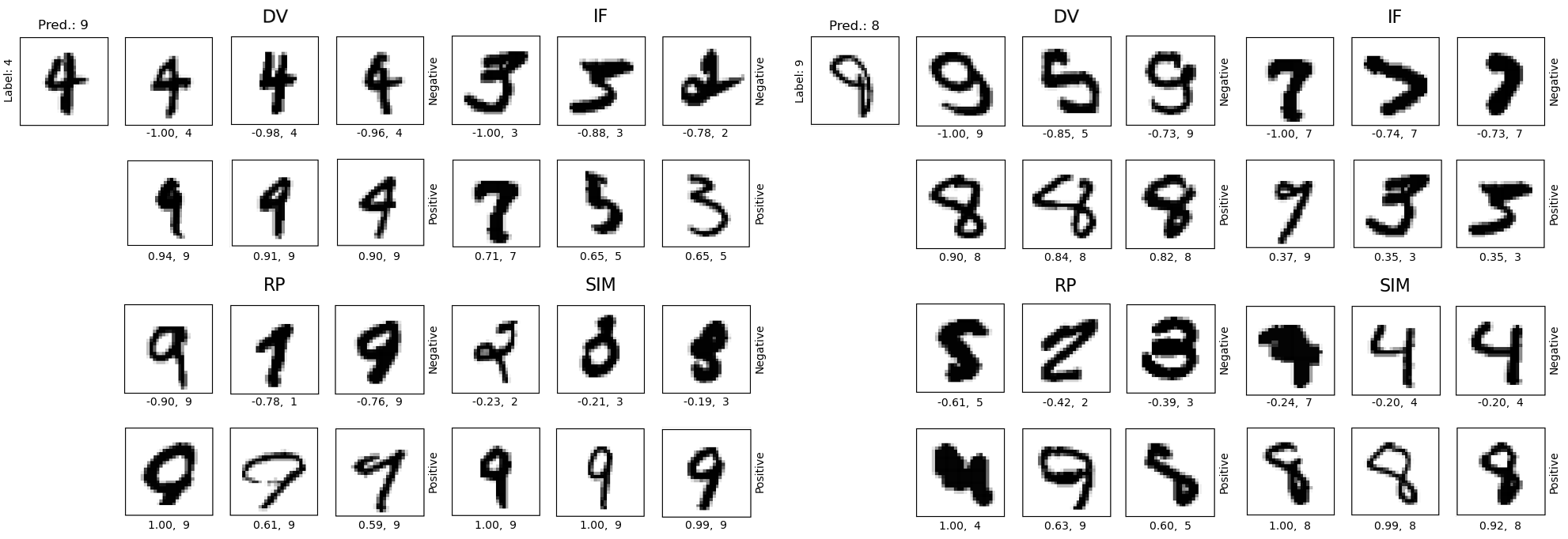
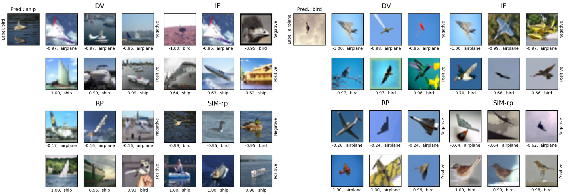
We evaluate the above explained methods on the MNIST LeCun, (1998) and CIFAR-10 Krizhevsky, (2009) datasets.²²2For both datasets, 2,000 test samples out of 10,000 have been randomly selected and used for validation purposes during training. These samples are excluded from all evaluations. For MNIST, a simple convolutional neural network with 3 convolutional and 3 fully connected layers with ReLU activations was used. For CIFAR-10, a modified implementation Phan, (2021) of the ResNet-18 architecture He et al., (2016) has been used. In all cases, we have used explanations for the decision class of the model. Figures 1 and 2 showcase example attributions by each of the methods for the MNIST and CIFAR-10 experiments, respectively. Appendix C includes more example explanations.

Refer to caption — Figure 1: Data attribution of two misclassified MNIST samples. The explanations are generated with respect to the decision class, which is indicated over the test sample on the left. The three examples shown are the most positively and negatively attributed training datapoints in each case. The upper row in each method’s explanations show training datapoints that are evidence against the decision (e.g. the test image on the left is not a 9 because of the training images in the upper rows), the bottom row shows images that are evidence for the decision. All attributions have been normalized to be in range $[-1,1]$ and indicated under the training instances, along with the label of the instance.

Because of the well-known high computational requirements for IF Schioppa et al., (2022); Hammoudeh and Lowd, (2023); Poché et al., (2023), we have restricted the computation of explanations to the final layer of the DNN, as in Koh and Liang, (2017). Inner product of parameter gradients also takes considerable time due to the high number of parameters of neural networks, especially for deep models Pruthi et al., (2020). Therefore, we do not report SIM results for CIFAR-10. However, we report an approximation of SIM explanations based on a random projection trick as explained by Pruthi et al., (2020), which we refer to as SIM-rp, for both datasets. We refer the reader to Appendix C for further details on SIM-rp and our evaluation procedures, including implementation details of the attribution methods and the evaluation metrics. Before presenting the evaluation results, we measure the computational requirements for each method in the next section.

5.3 Computational Resources

IF and SIM have non-negligible computational requirements. SIM-rp, on the other hand, uses a random projection of the parameters down to a space of $k$ dimensions to approximate SIM explanations. Letting $P$ be the number of parameters in the model, choosing $k\ll P$ greatly reduces the computational load. However, this procedure requires the allocation of memory to a random matrix ( in ${\mathbb{R}^{k\times P}}$ ), and to random projected gradients of the parameters (in ${\mathbb{R}^{k\times N}}$ ), adding additional memory requirements in the order of $O(k(P+N))$ . DV and RP both are very efficient in terms of both space and time. Both methods apply an inner product in the $p$ dimensional hidden feature space, and make use of a scalar number for each pair of training points and classes. To further reduce the required computation time, we pre-compute the hidden features of the training data points. This results in a total additional memory expense in the order of $O(N(p+C))$ .

While DV and RP are more run time efficient, both methods require a one-time surrogate pre-training phase. In order for the RPS decomposition of model weights to be applicable, model convergence is required. Therefore, after SGD training of the final layer, we perform fine-tuning with backtracking line search, using the GPU during the whole pre-training process Yeh et al., (2018). DV uses a quadratic programming solver which runs on a CPU.

SIM-rp also requires a pre-training phase to compute the lower dimensional representations of the training data point gradients. Table 1 contrasts the computational requirements of all considered approaches. We report the nominal values of the mean and standard deviations of pretraining times of 10 independent runs, and of explanation times of 50 test samples. We further report the required additional memory for our evaluation experiments. Computing SIM explanations on the CIFAR-10 dataset using the deep ResNet-18 model took more than $1.5$ hours for a single test sample, therefore we do not report SIM explanation times for CIFAR-10. All explanations have been generated on an NVidia Titan RTX GPU with the exception that the pretraining for DV has been done using the Shark Machine Learning Library Igel et al., (2008) using a 2.10 GHz Intel Xeon Gold 6130 CPU.

Table 1: We show pre-training run times, (local) explanation run times and additional memory requirements for each method and dataset. Time measurements are given in seconds. The mean and standard deviation of the measured time for 10 pretraining runs and 50 test sample explanations are reported. The additional memory requirements are given in MB (

1024^{2}

bytes). Note that among all compared methods, only DV has been pre-trained using a CPU. All other computations have been done on a GPU.

	Attribution Method	Pretraining Time		Explanation Time		Additional Memory
	Attribution Method	Mean	Std. Dev.	Mean	Std. Dev.	Additional Memory
MNIST	DV	$9.71$	$1.68$	$7.3\cdot 10^{-4}$	$6.5\cdot 10^{-5}$	$25.41$
	IF	–	–	$794.71$	$45.08$	–
	RPS	$30.21$	$1.82$	$7.0\cdot 10^{-4}$	$1.2\cdot 10^{-4}$	$25.41$
	SIM-rp	$269.35$	$11.28$	$2.7\cdot 10^{-3}$	$4.3\cdot 10^{-4}$	$645.78$
	SIM	–	–	$545.74$	$24.07$	–
CIFAR-10	DV	$42.12$	$7.03$	$0.0030$	$3.8\cdot 10^{-4}$	$21.17$
	IF	–	–	$784.88$	$54.33$	–
	RPS	$65.49$	$0.16$	$0.0032$	$5.6\cdot 10^{-4}$	$21.17$
	SIM-rp	$1066.96$	$25.34$	$0.016$	$0.018$	$5480.44$

The results showcase the high computational requirements of IF, even if we limit the explanations to the final layer parameters and use the approximation technique of Agarwal et al., (2017). While SIM-rp has low explanation time requirements, it has high memory requirements, in the order of several GBs for deep models.

DV and RPS are the most efficient methods in terms of additional memory requirements and the explanation times. For computing local data explanations, both methods are orders of magnitudes faster – by factors in the order of $10^{6}$ – compared to IF and SIM. In terms of the required memory usage, DV and RPS only depend on the number of training points and the number of final hidden features. This means that both methods scale much better than SIM-rp with respect to additional memory requirements, needing approximately $25$ times less memory for the shallow MNIST model, and $260$ times less memory for the deeper CIFAR-10 model. Compared to other methods depending on a pre-training step, DV is the fastest method in this category with RPS as a close second. However, both DV and RPS require considerably less training time compared to SIM-rp, resulting in an improvement of at least $16$ times for the CIFAR-10 experiments.

While RPS makes use of GPU computations to acheive short training times, DV uses a quadratic programming solver which runs on a CPU and results in lower training times. As such, it is the most energy efficient and least demanding method in all aspects of computational resources, among the methods considered here.

5.4 Evaluation Results

Table 2: Evaluation results for MNIST and CIFAR-10 datasets. For the Domain Mismatch Metric on the CIFAR-10 dataset, the trained model was robust against our perturbations, and thus we were able to use only 72 test samples. For all other evaluations, 4,000 test images have been used. Higher score is better for all metrics. Best results are in bold, and second best results are underlined. The expected score of a random attributor for each metric is given as RAND, assuming there is no class imbalance in the datasets, which is the case in our experiments.

	Attribution Method	Identical Class	Identical Subclass	Label Poisoning	Domain Mismatch
MNIST	DV	0.979	0.663	0.709	0.758
	IF	0.107	0.096	0.991	0.000
	RPS	0.763	0.300	0.499	1.000
	SIM-rp	0.979	0.968	0.108	0.947
	SIM	0.979	0.975	0.030	0.977
CIFAR-10	DV	0.868	0.486	0.826	0.430
	IF	0.835	0.480	0.907	0.000
	RPS	0.614	0.358	0.532	0.597
	SIM-rp	0.868	0.841	0.276	0.500
	RAND	0.100	0.100	0.500	0.030

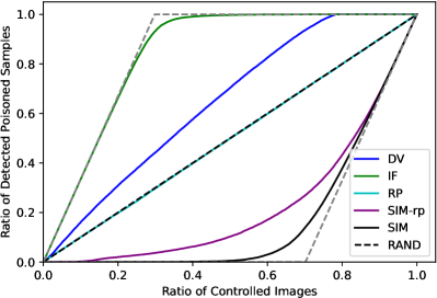
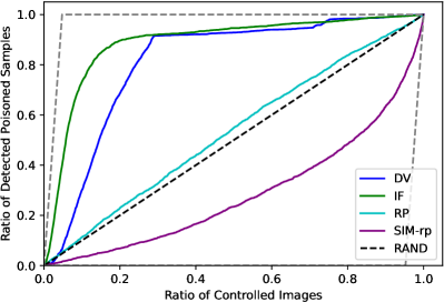
Table 2 presents all evaluation scores for the applied explanation quality metrics. Figure 3 presents line plots obtained for the Label Poisoning Experiment metric. SIM performs well in the class matching tests of Identical Class, Identical Subclass and Domain Mismatch tests. However, it severely underperforms in the Label Poisoning Experiment. RP consistently performs at a random level for this metric, and is the best method in terms of Domain Mismatch Test.

In the majority of the cases, DV explanations are either the best or the second best candidate. DV obtains comparable scores that are better than a random performance in all cases. Thus, it has competitive performance across evaluation metrics and datasets.

IF scores remarkably high in the Label Poisoning Experiment metric. IF reportedly attributes greater relevance to datapoints with high loss Koh and Liang, (2017); Poché et al., (2023). Therefore, IF can be used to detect mislabeled examples or outliers Feldman and Zhang, (2020), and its high scores on the Label Poisoning Experiment metric verify this. Interestingly, IF performs at a random level for the Identical Class and Subclass Test metrics on MNIST, while it has high scores for CIFAR-10. We hypothesize this is related to the much lower number of parameters in the final layer of our MNIST model.

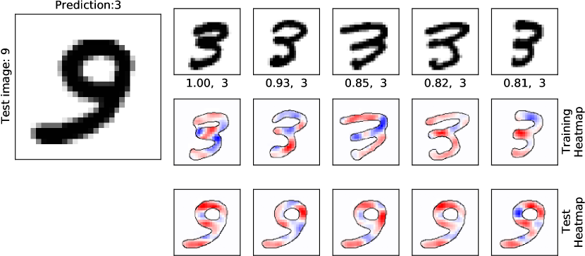
6 Combining Data Attribution and Feature Attribution with DualView

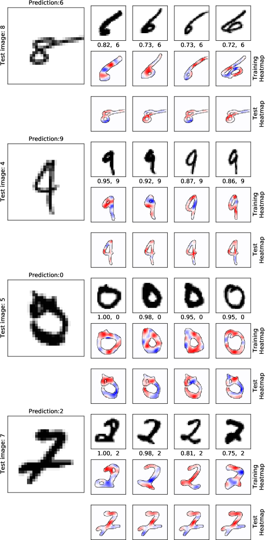
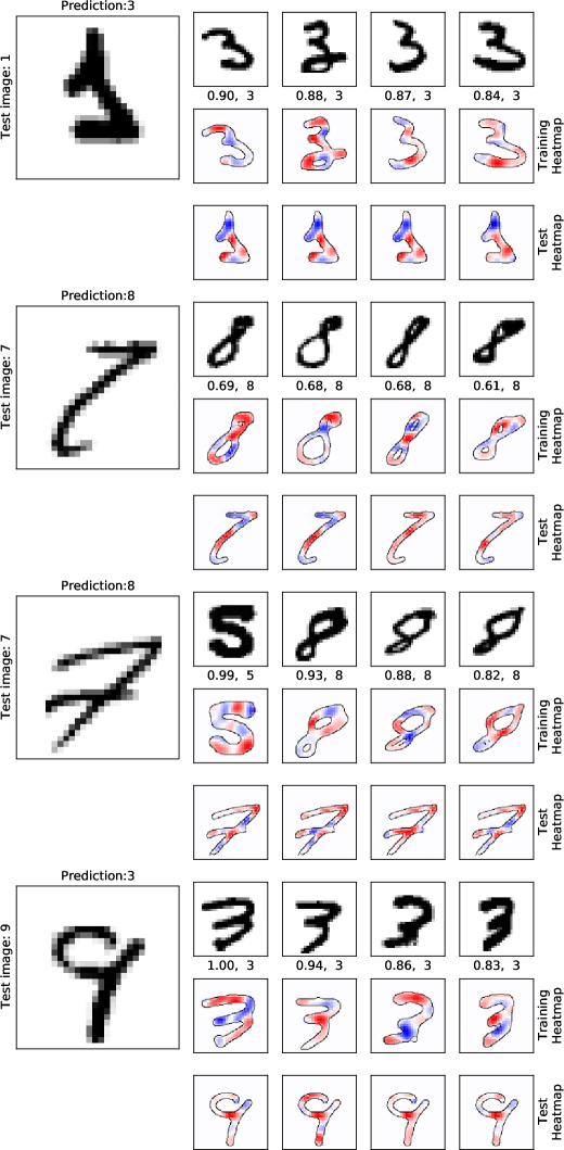
In this section, we combine feature attribution techniques and data attribution approaches to obtain explanations in terms of feature level attributions, simultaneously for both the test point and the most influential training samples. To our knowledge, this is the first work to propose a strategy to produce local data attribution explanations values in the test and training feature level, indicating which parts of the training data is responsible for model decisions on test points.

DualView decomposes the output of the surrogate model into contributions of each training data point, such that the model output is equal to the sum of all relevance scores of training points. Each relevance computation contains an inner product of final layer features. We can further decompose this inner product to the contributions of each feature. We use these values to initialize feature-level explanations via Layer-wise Relevance Propagation (LRP) Bach et al., (2015) at the penultimate layer.

LRP Bach et al., (2015) is a feature attribution technique based on computing lower layer feature relevances using the relevances of upper layer features by manner of step-wise proportional decomposition, such that the total sum of relevance scores is conserved across layers of computation, preserving a connection between the quantity initially back-propagated, and the resulting explanation. At the end of this procedure, we obtain relevance values for each input feature. In the image domain, this is commonly represented as a heatmap over the corresponding input.

As such, by applying LRP onto the explanations obtained via DV at the penultimate layer, we unify the notion of data attribution relevance and feature attribution relevance to provide explanations in the test feature space, as well as the training data feature space.

Concretely, given a test point $\mathbf{x}_{\text{test}}$ , with penultimate layer output $\mathbf{f}^{\text{test}}\in\mathbb{R}^{p}$ ; a training datapoint $\mathbf{x}_{\text{i}}$ , with penultimate layer output $\mathbf{f}^{\text{i}}\in\mathbb{R}^{p}$ and label $y_{i}$ ; we set the initial relevance of the $k^{\text{th}}$ feature in the penultimate layer

R^{k}(\mathbf{x})=\left\{\begin{array}[]{ll}(\sum_{j\neq c}\lambda_{ij})\mathbf{f}_{k}^{\text{test}}\mathbf{f}_{k}^{\text{i}}&\mbox{if }y_{i}=c\\ -\lambda_{ic}\mathbf{f}_{k}^{\text{test}}\mathbf{f}_{k}^{\text{i}}&\mbox{else}\end{array}\right.

(7)

Figure 4 presents an example. By further applying LRP to the sum-components of the DV explanations related to each show test point, we can recognize that the model is matching three horizontal strokes of the different training images of the digit $3$ to the parts of the slanted digit $9$ shown in the test image. Additional explanations similar to the one shown in Figure 4 can be found in Appendix C.

7 Conclusion

In this paper, we have proposed DualView, a local data attribution method based on the decomposition of model outputs using a margin maximizing kernel surrogate classifier, which utilizes the final hidden layer representations as the kernel. We have evaluated DualView against prominent methods from the literature using concrete quantitative evaluation metrics, each measuring a different desirable property of local data attribution explanations.

Our results demonstrate that DualView is the most efficient method by far in terms of its use of computational resources in both space and time (and therefore energy). Furthermore, our method shows competitive performance across all explanation quality evaluation metrics. That is, while other methods might perform best in some scenarios, they tend to underperform considerably in other tests. Only DV performs competently across all evaluation scenarios. Therefore it constitutes a reliable and practically feasible-to-use data attribution strategy, due to itsenergy efficiency and configurability in terms of pre-training time and sparsity of explanations.

Moreover, DualView allows us to combine feature attribution and data attribution approaches to go beyond data attribution. This approach unveils the interaction between the test and training features and shows us why the training points are relevant for the neural network decision.

Acknowledgement

This work was supported by the Federal Ministry of Education and Research (BMBF) as grant BIFOLD (01IS18025A, 01IS180371I); the German Research Foundation (DFG) as research unit DeSBi (KI-FOR 5363); the European Union’s Horizon Europe research and innovation programme (EU Horizon Europe) as grant TEMA (101093003); the European Union’s Horizon 2020 research and innovation programme (EU Horizon 2020) as grant iToBoS (965221); and the state of Berlin within the innovation support programme ProFIT (IBB) as grant BerDiBa (10174498).

References

Adebayo et al., (2018) Adebayo, J., Gilmer, J., Muelly, M., Goodfellow, I., Hardt, M., and Kim, B. (2018). Sanity checks for saliency maps. In Bengio, S., Wallach, H., Larochelle, H., Grauman, K., Cesa-Bianchi, N., and Garnett, R., editors, Advances in Neural Information Processing Systems, volume 31. Curran Associates, Inc.
Agarwal et al., (2017) Agarwal, N., Bullins, B., and Hazan, E. (2017). Second-order stochastic optimization for machine learning in linear time. Journal of Machine Learning Research, 18(116):1–40.
Bach et al., (2015) Bach, S., Binder, A., Montavon, G., Klauschen, F., Müller, K.-R., and Samek, W. (2015). On pixel-wise explanations for non-linear classifier decisions by layer-wise relevance propagation. PloS one, 10(7):e0130140.
Barshan et al., (2020) Barshan, E., Brunet, M.-E., and Dziugaite, G. K. (2020). Relatif: Identifying explanatory training samples via relative influence. In Chiappa, S. and Calandra, R., editors, Proceedings of the Twenty Third International Conference on Artificial Intelligence and Statistics, volume 108 of Proceedings of Machine Learning Research, pages 1899–1909. PMLR.
Bien and Tibshirani, (2011) Bien, J. and Tibshirani, R. (2011). Prototype selection for interpretable classification. The Annals of Applied Statistics, 5(4).
Brophy, (2020) Brophy, J. (2020). Exit through the training data: A look into instance-attribution explanations and efficient data deletion methods in machine learning models.
Charpiat et al., (2019) Charpiat, G., Girard, N., Felardos, L., and Tarabalka, Y. (2019). Input similarity from the neural network perspective. In Wallach, H., Larochelle, H., Beygelzimer, A., d'Alché-Buc, F., Fox, E., and Garnett, R., editors, Advances in Neural Information Processing Systems, volume 32. Curran Associates, Inc.
Chen et al., (2021) Chen, Y., Li, B., Yu, H., Wu, P., and Miao, C. (2021). HYDRA: hypergradient data relevance analysis for interpreting deep neural networks. CoRR, abs/2102.02515.
Crammer and Singer, (2001) Crammer, K. and Singer, Y. (2001). On the algorithmic implementation of multiclass kernel-based vector machines. Journal of machine learning research, 2(Dec):265–292.
Engel et al., (2023) Engel, A., Wang, Z., Frank, N. S., Dumitriu, I., Choudhury, S., Sarwate, A., and Chiang, T. (2023). Faithful and efficient explanations for neural networks via neural tangent kernel surrogate models.
Feldman and Zhang, (2020) Feldman, V. and Zhang, C. (2020). What neural networks memorize and why: Discovering the long tail via influence estimation. In Larochelle, H., Ranzato, M., Hadsell, R., Balcan, M., and Lin, H., editors, Advances in Neural Information Processing Systems, volume 33, pages 2881–2891. Curran Associates, Inc.
Gidel et al., (2019) Gidel, G., Bach, F., and Lacoste-Julien, S. (2019). Implicit regularization of discrete gradient dynamics in linear neural networks. In Wallach, H., Larochelle, H., Beygelzimer, A., d'Alché-Buc, F., Fox, E., and Garnett, R., editors, Advances in Neural Information Processing Systems, volume 32. Curran Associates, Inc.
Gunasekar et al., (2018) Gunasekar, S., Lee, J. D., Soudry, D., and Srebro, N. (2018). Implicit bias of gradient descent on linear convolutional networks. In Bengio, S., Wallach, H., Larochelle, H., Grauman, K., Cesa-Bianchi, N., and Garnett, R., editors, Advances in Neural Information Processing Systems, volume 31. Curran Associates, Inc.
Haim et al., (2022) Haim, N., Vardi, G., Yehudai, G., Shamir, O., and Irani, M. (2022). Reconstructing training data from trained neural networks.
Hammoudeh and Lowd, (2023) Hammoudeh, Z. and Lowd, D. (2023). Training data influence analysis and estimation: A survey.
Han et al., (2020) Han, X., Wallace, B. C., and Tsvetkov, Y. (2020). Explaining black box predictions and unveiling data artifacts through influence functions. In Jurafsky, D., Chai, J., Schluter, N., and Tetreault, J., editors, Proceedings of the 58th Annual Meeting of the Association for Computational Linguistics, pages 5553–5563, Online. Association for Computational Linguistics.
Hanawa et al., (2021) Hanawa, K., Yokoi, S., Hara, S., and Inui, K. (2021). Evaluation of similarity-based explanations. In International Conference on Learning Representations.
Hayashi, (2022) Hayashi, Y. (2022). Emerging trends in deep learning for credit scoring: A review. Electronics, 11(19):3181.
He et al., (2016) He, K., Zhang, X., Ren, S., and Sun, J. (2016). Deep residual learning for image recognition. In 2016 IEEE Conference on Computer Vision and Pattern Recognition (CVPR), pages 770–778.
Hedström et al., (2023) Hedström, A., Weber, L., Krakowczyk, D., Bareeva, D., Motzkus, F., Samek, W., Lapuschkin, S., and Höhne, M. M.-C. (2023). Quantus: An explainable ai toolkit for responsible evaluation of neural network explanations and beyond. Journal of Machine Learning Research, 24(34):1–11.
Hu et al., (2018) Hu, Z., Tang, J., Wang, Z., Zhang, K., Zhang, L., and Sun, Q. (2018). Deep learning for image-based cancer detection and diagnosis- a survey. Pattern Recognition, 83:134–149.
Igel et al., (2008) Igel, C., Heidrich-Meisner, V., and Glasmachers, T. (2008). Shark. Journal of Machine Learning Research, 9:993–996.
Ilyas et al., (2022) Ilyas, A., Park, S. M., Engstrom, L., Leclerc, G., and Madry, A. (2022). Datamodels: Understanding predictions with data and data with predictions. In Chaudhuri, K., Jegelka, S., Song, L., Szepesvari, C., Niu, G., and Sabato, S., editors, Proceedings of the 39th International Conference on Machine Learning, volume 162 of Proceedings of Machine Learning Research, pages 9525–9587. PMLR.
Iwata and Yoshikawa, (2021) Iwata, T. and Yoshikawa, Y. (2021). Training deep models to be explained with fewer examples. ArXiv, abs/2112.03508.
Ji and Telgarsky, (2018) Ji, Z. and Telgarsky, M. (2018). Gradient descent aligns the layers of deep linear networks. CoRR, abs/1810.02032.
Ji and Telgarsky, (2020) Ji, Z. and Telgarsky, M. (2020). Directional convergence and alignment in deep learning. In Larochelle, H., Ranzato, M., Hadsell, R., Balcan, M., and Lin, H., editors, Advances in Neural Information Processing Systems, volume 33, pages 17176–17186. Curran Associates, Inc.
Karim et al., (2022) Karim, M. R., Shajalal, M., Graß, A., Döhmen, T., Chala, S. A., Beecks, C., and Decker, S. (2022). Interpreting black-box machine learning models for high dimensional datasets.
Koh and Liang, (2017) Koh, P. W. and Liang, P. (2017). Understanding black-box predictions via influence functions. In Precup, D. and Teh, Y. W., editors, Proceedings of the 34th International Conference on Machine Learning, volume 70 of Proceedings of Machine Learning Research, pages 1885–1894. PMLR.
Krizhevsky, (2009) Krizhevsky, A. (2009). Learning multiple layers of features from tiny images. pages 32–33.
Kuhn, (1951) Kuhn, T. A. (1951). Hw nonlinear programming. In Proceedings of 2nd Berkeley Symposium. Berkeley: University of California Press, pages 481–492.
Lapuschkin et al., (2019) Lapuschkin, S., Wäldchen, S., Binder, A., Montavon, G., Samek, W., and Müller, K.-R. (2019). Unmasking clever hans predictors and assessing what machines really learn. Nature communications, 10(1):1096.
LeCun, (1998) LeCun, Y. (1998). The mnist database of handwritten digits. http://yann. lecun. com/exdb/mnist/.
Lyu and Li, (2019) Lyu, K. and Li, J. (2019). Gradient descent maximizes the margin of homogeneous neural networks. CoRR, abs/1906.05890.
Mehdi and Tiwary, (2023) Mehdi, S. and Tiwary, P. (2023). Thermodynamics of interpretation.
Park et al., (2023) Park, S. M., Georgiev, K., Ilyas, A., Leclerc, G., and Madry, A. (2023). Trak: attributing model behavior at scale. In Proceedings of the 40th International Conference on Machine Learning, ICML’23. JMLR.org.
Paszke et al., (2019) Paszke, A., Gross, S., Massa, F., Lerer, A., Bradbury, J., Chanan, G., Killeen, T., Lin, Z., Gimelshein, N., Antiga, L., Desmaison, A., Kopf, A., Yang, E., DeVito, Z., Raison, M., Tejani, A., Chilamkurthy, S., Steiner, B., Fang, L., Bai, J., and Chintala, S. (2019). Pytorch: An imperative style, high-performance deep learning library. In Wallach, H., Larochelle, H., Beygelzimer, A., d'Alché-Buc, F., Fox, E., and Garnett, R., editors, Advances in Neural Information Processing Systems, volume 32. Curran Associates, Inc.
Pezeshkpour et al., (2021) Pezeshkpour, P., Jain, S., Wallace, B., and Singh, S. (2021). An empirical comparison of instance attribution methods for NLP. In Toutanova, K., Rumshisky, A., Zettlemoyer, L., Hakkani-Tur, D., Beltagy, I., Bethard, S., Cotterell, R., Chakraborty, T., and Zhou, Y., editors, Proceedings of the 2021 Conference of the North American Chapter of the Association for Computational Linguistics: Human Language Technologies, pages 967–975, Online. Association for Computational Linguistics.
Phan, (2021) Phan, H. (2021). huyvnphan/pytorch_cifar10.
Poché et al., (2023) Poché, A., Hervier, L., and Bakkay, M.-C. (2023). Natural Example-Based Explainability: a Survey. In World Conference on eXplainable Artificial Intelligence, Lisbon, Portugal.
Pruthi et al., (2020) Pruthi, G., Liu, F., Kale, S., and Sundararajan, M. (2020). Estimating training data influence by tracing gradient descent. In Larochelle, H., Ranzato, M., Hadsell, R., Balcan, M., and Lin, H., editors, Advances in Neural Information Processing Systems, volume 33, pages 19920–19930. Curran Associates, Inc.
Ribeiro et al., (2016) Ribeiro, M. T., Singh, S., and Guestrin, C. (2016). ”why should i trust you?”: Explaining the predictions of any classifier. In Proceedings of the 22nd ACM SIGKDD International Conference on Knowledge Discovery and Data Mining, KDD ’16, page 1135–1144, New York, NY, USA. Association for Computing Machinery.
Samek et al., (2017) Samek, W., Binder, A., Montavon, G., Lapuschkin, S., and Müller, K.-R. (2017). Evaluating the visualization of what a deep neural network has learned. IEEE Transactions on Neural Networks and Learning Systems, 28(11):2660–2673.
Schioppa et al., (2022) Schioppa, A., Zablotskaia, P., Vilar, D., and Sokolov, A. (2022). Scaling up influence functions. In Proceedings of the AAAI Conference on Artificial Intelligence, volume 36, pages 8179–8186.
Soudry et al., (2018) Soudry, D., Hoffer, E., Nacson, M. S., Gunasekar, S., and Srebro, N. (2018). The implicit bias of gradient descent on separable data. volume 19, pages 1–57.
Srikantan, (1961) Srikantan, K. S. (1961). Testing for the single outlier in a regression model. Sankhyā: The Indian Journal of Statistics, Series A (1961-2002), 23(3):251–260.
Tarzanagh et al., (2023) Tarzanagh, D. A., Li, Y., Thrampoulidis, C., and Oymak, S. (2023). Transformers as support vector machines.
Tolan et al., (2019) Tolan, S., Miron, M., Gómez, E., and Castillo, C. (2019). Why machine learning may lead to unfairness: Evidence from risk assessment for juvenile justice in Catalonia. In Proceedings of the Seventeenth International Conference on Artificial Intelligence and Law, pages 83–92.
Yeh et al., (2018) Yeh, C., Kim, J. S., Yen, I. E., and Ravikumar, P. (2018). Representer point selection for explaining deep neural networks. CoRR, abs/1811.09720.
Yeh et al., (2019) Yeh, C.-K., Hsieh, C.-Y., Suggala, A., Inouye, D. I., and Ravikumar, P. K. (2019). On the (in)fidelity and sensitivity of explanations. In Wallach, H., Larochelle, H., Beygelzimer, A., d'Alché-Buc, F., Fox, E., and Garnett, R., editors, Advances in Neural Information Processing Systems, volume 32. Curran Associates, Inc.

Appendix

Appendix A Derivation of Equation (6)

Given the soft-margin optimization problem of Crammer and Singer, (2001)

\begin{array}[]{llllll}\min_{W}&\lx@intercol\frac{1}{2}||W||^{2}_{2}+K\sum_{i=1}^{N}\xi_{i}\hfil\lx@intercol\\ \textrm{s.t.}&\forall i\in[N],\forall j\in[C]\\ &(w_{y_{i}}^{T}\mathbf{x}_{i})-(w_{j}^{T}\mathbf{x}_{i})+\delta_{jy_{i}}\geq 1-\xi_{i}\\ \end{array}

(8)

where $\delta_{xy}$ denotes the Kroenecker delta function, we derive the Lagrangian:

\mathcal{L}(W,\xi,\mathcal{D},\lambda)=\frac{1}{2}\sum_{i=1}^{C}||w_{i}||^{2}_{2}+K\sum_{i=1}^{N}\xi_{i}+\sum_{i=1}^{N}\sum_{j=1}^{C}\lambda_{ij}\big{[}(w_{j}-w_{y_{i}})^{T}\mathbf{x}_{i}+1-\delta_{jy_{i}}-\xi_{i}\big{]}

(9)

Then taking derivatives with respect to the primal variables to enforce the stationarity condition Kuhn, (1951):

	$\displaystyle\forall i\in[N],\frac{\partial\mathcal{L}}{\partial\xi_{i}}=K-\sum_{j=1}^{C}\lambda_{ij}=0\implies\forall i\in[N],\sum_{j=1}^{C}\lambda_{ij}=K$		(10)
	$\displaystyle\frac{\partial\mathcal{L}}{\partial w_{k}}=w_{k}+\sum_{i=1}^{N}\lambda_{ik}\mathbf{x}_{i}-\sum_{i:y_{i}=k}\underbrace{\sum_{j=1}^{C}\lambda_{ij}}_{=K\text{by Eq. \eqref{eq:sum_of_dual_vars}}}\mathbf{x}_{i}=0$		(11)
	$\displaystyle\implies\forall k\in[C],w_{k}=\sum_{i=1}^{N}(K\delta_{y_{i},k}-\lambda_{ik})\mathbf{x}_{i}$		(12)

From Equations (10) and (12) we derive:

\forall i\in[N],\sum_{j=1}^{C}\lambda_{ij}=K\implies\forall i\in[N],K-\lambda_{iy_{i}}=\sum_{j:y_{i}\neq j}\lambda_{ij}

(13)

\forall j\in[C],w_{j}=\sum_{i=1}^{N}(K\delta_{y_{i},j}-\lambda_{ij})\mathbf{f}_{i}=\sum_{i:y_{i}=j}(K-\lambda_{iy_{i}})\mathbf{f}_{i}-\sum_{i:y_{i}\neq j}\lambda_{ij}\mathbf{f}_{i}

(14)

Combining these two results, we have:

w_{j}=\sum_{i:y_{i}=j}(\sum_{k:y_{i}\neq k}\lambda_{ik})\mathbf{f}_{i}-\sum_{i:y_{i}\neq j}\lambda_{ij}\mathbf{f}_{i}

(15)

As such, the output of the surrogate model on input $\mathbf{x}$ is given by:

\forall j\in[C],\Phi(\mathbf{x};\mathbf{\vartheta},W)_{j}=w_{j}^{T}\mathbf{f}(\mathbf{x};\mathbf{\vartheta})=\sum_{i:y_{i}=j}(\sum_{k:y_{i}\neq k}\lambda_{ik})\mathbf{f}^{T}_{i}\mathbf{f}(\mathbf{x};\mathbf{\vartheta})-\sum_{i:y_{i}\neq j}\lambda_{ij}\mathbf{f}^{T}_{i}\mathbf{f}(\mathbf{x};\mathbf{\vartheta})

(16)

Thus, the output of the network for any class is a linear combination of the inner products of the test point with training points. This motivates our choice in Equation (6).

To solve this problem, we can find the dual problem by plugging Equation (15) in the Lagrangian and maximize it subject to the dual feasibility conditions Kuhn, (1951) $\forall i\in[N],\forall j\in[C],\lambda_{ij}\geq 0$ . We refer the reader to Crammer and Singer, (2001) for the derivations.

After solving this problem, we obtain a non-negative real matrix $\mathbf{\Lambda}\in\mathbb{R}_{+}^{N\times C}$ , consisting of the dual variables, which constitute the coefficients of each training datapoint in the final decision vector. Each row $i$ of $\mathbf{\Lambda}$ corresponds to a training datapoint $\mathbf{x}_{i}$ .

Each datapoint $\mathbf{x}_{i}$ contributes negatively to decisions for classes other than its own class $y_{i}$ (classes $j\neq y_{i}$ ), and the coefficient for this contribution is $\lambda_{ij}$ .

Each datapoint $\mathbf{x}_{i}$ contributes positively to decisions for its own classes ( $j=y_{i}$ ), and the coefficient for this contribution is the sum of the multipliers for other classes: $\sum_{k\neq y_{i}}\lambda_{ik}$ . Due to the way the multiclass SVM is defined, there are no dual variables $\lambda_{iy_{i}}$ corresponding to model decisions. In the derivations above, the variables $\lambda_{iy_{i}}$ are introduced by the soft margin generalization. They correspond to the condition that slack variables are positive and they are simply the values that satisfy Equation (10). The corresponding coefficient for decisions of class $y_{i}$ for a training datapoint $\mathbf{x}_{i}$ is the sum of the dual variables corresponding to other classes, which is induced by the choice of sharing slack variables across classes for each training datapoint as defined by Crammer and Singer, (2001).

Note that only a subset of the training data will have positive attributions, since all the datapoints outside the margin will have all $0$ values in the corresponding rows of $\mathbf{\Lambda}$ . This formulation is equivalent to using the feature extractor part of the neural network as a kernel in the multiclass vector machine formulation.

Appendix B Effect of Hyperparameter $K$

Data attributions explanations can be cognitively hard to process, especially if too many datapoints are attributed comparable relevances in the training dataset, which is usually massive with millions of examples in practical settings. Iwata and Yoshikawa, (2021) report that RPS explanations are generally too hard to interpret because of the high number of relevant training datapoints. They suggest a strategy to obtain sparser explanations. However, too much sparsity hurts the expressivity of explanations, resulting in too few relevant examples which may not capture all aspects of the reasoning employed by the ML model.

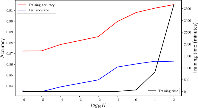
Our choice of surrogate model is tunable via the hyperparemeter $K$ in two complementary aspects. Increasing $K$ corresponds to using a harder margin to train the surrogate margin maximizing classifier. This results in a reduced number of support vectors, which indicates sparser explanations of low complexity. However, the low number of support vectors necessitate a longer training time. In this appendix we quantify this tradeoff. Since we noticed that small changes in the hyperparameter does not result in sizable differences in terms of training time and sparsity, we report values on a logarithmic scale. We report the number of support vectors for each class and the training time for $K=10^{k}$ where $k\in\{-6,-5,-4,-3,-2,-1,0,1,2\}$ .

Results

Table 3 lists the surrogate model’s training times using the Shark Machine Learning library Igel et al., (2008). We report the training time in minutes. The results are given in Table 3. The same information is also visualized in Figures 5.b and 6.b. Figures 5.a and 6.a show the number of support vectors for each class, for each value of K.

Table 3: Training times and train and test accuracies of DualView surrogate models on a CPU with different values of the hyperparameter

K

. The training times are reported in minutes.

	$\mathbf{log_{10}K}$	$-6$	$-5$	$-4$	$-3$	$-2$	$-1$	$0$	$1$	$2$
MNIST	Train time	0.68	0.52	0.68	2.33	8.81	30.73	148.48	950.24	1113.66
	Train acc.	0.955	0.980	0.990	0.995	0.996	0.997	0.998	0.999	0.999
	Test acc.	0.951	0.971	0.980	0.982	0.982	0.980	0.978	0.976	0.975
CIFAR-10	Train time	1.11	1.07	0.94	0.81	1.34	9.31	70.28	832.49	3667.93
	Train acc.	0.872	0.873	0.878	0.882	0.886	0.900	0.908	0.912	0.915
	Test acc.	0.835	0.835	0.839	0.842	0.846	0.858	0.860	0.863	0.862

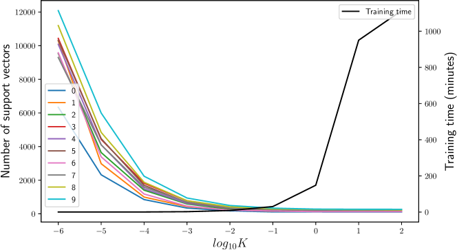
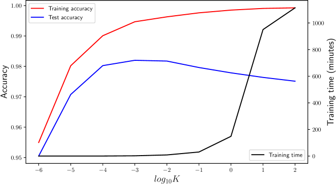
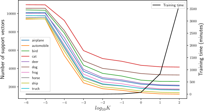
Discussion

The results verify the argument on the tunability of our choice of surrogate model in terms of training time and sparsity of the explanations. We see that the number of support vectors are close to each other across different classes for all $K$ values, and it decreases with increasing $K$ values. Contrarily, the training times increase with increasing $K$ values.

Another noticeable detail is that the number of support vectors seem to converge for $K>10^{-3}$ . This can be observed in the results of both datasets. Furthermore, we note that training times are relatively stable for $K<10^{-3}$ , whereas they diverge for bigger $K$ . This suggests a sweet spot at around $K=10^{-3}$ , which achieves sparse explanations with low training time, with enough support vectors to produce expressive explanations.

Appendix C Details of the Evaluation Experiments and Additional Examples of Explanations

This section clarifies implementational details and provides additional example explanations of misclassified samples.

C.1 Implementational Details of Methods

For IF explanations using the method of Agarwal et al., (2017), we have used an open-source Pytorch Paszke et al., (2019) implementation of the method³³3https://github.com/ryokamoi/pytorch_influence_functions. The suggested minimal hyperparameters have been used to compute reliable approximations of the inverse Hessian product in the shortest time. For RP explanations, we have used the official code release⁴⁴4https://github.com/chihkuanyeh/Representer_Point_Selection for the original paper Yeh et al., (2018). To train our surrogate models, we have used a C++ implementation using the Shark Machine Learning Library Igel et al., (2008) to solve the quadratic program given in (5). We have modified this implementation to access the dual variables of the solution. We have implemented SIM in a straightforward fashion.

For SIM-rp explanations, we have used the random projection trick from Pruthi et al., (2020). Letting $P$ denote the number of model parameters, this method consists of sampling a matrix $G\in\mathbb{R}^{k\times P}$ such that each entry is independently sampled from a normal distribution $\mathcal{N}(0,\frac{1}{k})$ so that $\mathbb{E}(G^{\top}G)=\mathbf{I}$ . As such, $\nabla_{\theta}\Phi(\mathbf{x};\theta)_{c}^{\top}G^{\top}G\nabla_{\theta}\Phi(\mathbf{x}_{i};\theta)_{y_{i}}$ is an unbiased estimate of $\nabla_{\theta}\Phi(\mathbf{x};\theta)_{c}^{\top}\nabla_{\theta}\Phi(\mathbf{x}_{i};\theta)_{y_{i}}$ . Selecting $k\ll P$ results in a big improvement in explanations times. Although sampling many $G$ and taking the mean of the explanations results in an estimator of lower variance, it requires more additional storage, which is already in the order of GBs for a single $G$ . Moreover, we have found empirically that this ameliorates the evaluation scores marginally. Therefore, we have only used one sample of $G$ . We have selected $k=128$ for experiments on both datasets.

C.2 Implementational Details of Evaluation Metrics

For the Label Poisoning Experiment evaluations on the MNIST dataset, we have poisoned a ratio of $0.3$ of the training datapoints at random. With a deeper model on CIFAR-10, model training became difficult with that ratio of poisoned labels. We have reduced the ratio to $0.03$ . Hence the difference in the best and worst curves for the two datasets.

For the Domain Mismatch Test metric, we have perturbed a ratio of $0.3$ of training samples from the third class in both datasets. This corresponds to the class 2 in MNIST and the class bird in CIFAR-10. As the constant perturbation, we have opted to add a square frame around the images, and a small square in the middle, to allow the model to detect the perturbation in different parts of the input image. Figure 7 showcases two perturbed training images.