Universal Generalization Guarantees for Wasserstein Distributionally Robust Models

Abstract

Distributionally robust optimization has emerged as an attractive way to train robust machine learning models, capturing data uncertainty and distribution shifts. Recent statistical analyses have proved that robust models built from Wasserstein ambiguity sets have nice generalization guarantees, breaking the curse of dimensionality. However, these results are obtained in specific cases, at the cost of approximations, or under assumptions difficult to verify in practice. In contrast, we establish, in this article, exact generalization guarantees that cover all practical cases, including any transport cost function and any loss function, potentially non-convex and nonsmooth. For instance, our result applies to deep learning, without requiring restrictive assumptions. We achieve this result through a novel proof technique that combines nonsmooth analysis rationale with classical concentration results. Our approach is general enough to extend to the recent versions of Wasserstein/Sinkhorn distributionally robust problems that involve (double) regularizations.

1 Introduction

1.1 Wasserstein robustness: models and generalization

Machine learning models are challenged in practice by many obstacles, such as biases in data, adversarial attacks, or data shifts between training and deployment. Towards more resilient and reliable models, distributionally robust optimization has emerged as an attractive paradigm, where training no longer relies on minimizing the empirical risk, but rather on an optimization problem that takes into account potential perturbations in the data distribution; see e.g., the review articles [23, 9].

More specifically, the approach consists in minimizing the worst-risk among all distributions in a neighborhood of the empirical data distribution. A natural way [27] to define such a neighborhood is to use the optimal transport distance, called the Wasserstein distance [28]. Between two distributions $Q$ and $Q^{\prime}$ on a sample space $\Xi$, the Wasserstein distance is defined as the minimal expected cost among all coupling probability $\pi$ on $\Xi\times\Xi$ having $Q$ and $Q^{\prime}$ as marginals:

$$W_{c}(Q,Q^{\prime}):=\inf_{\begin{subarray}{c}\pi\in\mathcal{P}(\Xi\times\Xi)\\ [\pi]_{1}=Q,[\pi]_{2}=Q^{\prime}\end{subarray}}\mathbb{E}_{(\xi,\zeta)\sim\pi}[c(\xi,\zeta)],$$ (1)

where $c\colon\Xi\times\Xi\rightarrow\mathbb{R}$ is a transport cost over the sample space $\Xi$. For a class of loss functions $\mathcal{F}$, the Wasserstein distributionally robust counterpart of the standard empirical risk minimization then writes

$$\min_{f\in\mathcal{F}}~{}~{}\max_{Q\in\mathcal{P}(\Xi),W_{c}(\widehat{P}_{n},Q)\leq\rho}\mathbb{E}_{\xi\sim Q}[f(\xi)],$$ (2)

for a chosen radius $\rho$ of the Wasserstein ball centered at the empirical data distribution, denoted $\widehat{P}_{n}$. In the degenerate case $\rho=0$, we have $Q=\widehat{P}_{n}$ and (2) boils down to empirical risk minimization. If $\rho>0$, the training captures data uncertainty and provides more resilient learning models; see the discussions and illustrations [33, 35, 39, 24, 26, 36, 20, 4, 7].

To support theoretically the modeling versatility and the practical success of these robust models, some statistical guarantees have been proposed in the literature. For a population distribution $P$, i.i.d. samples $\xi_{1},\ldots,\xi_{n}$ drawn from $P$, and the associated empirical distribution $\widehat{P}_{n}:=\frac{1}{n}\sum_{i=1}^{n}\delta_{\xi_{i}}$, the best concentration results for the Wasserstein distance [18] gives that if the radius $\rho$ is large enough, then the Wasserstein ball around $\widehat{P}_{n}$ contains the true distribution $P$ with high probability, which in turn gives directly [27] a generalization bound of the form

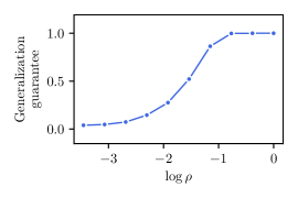
Figure 1: Probability of the generalization bound (3) to hold, estimated from 500 logistic regression instances and their $\ell_{1}$-robust counterparts (see at the end of Section 3). For large $\rho$, the bound always holds, whereas it does not for small $\rho$. Our aim is to quantify this phenomenon, which is not explained by existing results.

$$\max_{Q\in\mathcal{P}(\Xi),W_{c}(\widehat{P}_{n},Q)\leq\rho}\mathbb{E}_{\xi\sim Q}[f(\xi)]\geq\mathbb{E}_{\xi\sim P}[f(\xi)].$$ (3)

This exact bound is particularly attractive: the quantity that we compute from data and optimize by training provides a control on the idealistic population risk. However, the direct application of [18] requires a number of training samples growing exponentially in the dimension.

Recent works have improved this direct approach by establishing, in various situations, generalization bounds that do not suffer from the curse of dimensionality, and rather feature radius $\rho$ scaling as $O(1/\sqrt{n})$ [35, 10, 3, 19, 5, 11]. Yet no existing result is general enough to cover all situations encountered in machine learning and to explain nice generalization properties usually observed in practice (as illustrated in Figure 1).

1.2 Contributions and outline

In this paper, we provide exact generalization guarantees of the form (3), that are universal, in the sense that they apply to all machine learning situations, without restrictive assumptions. Indeed, our results apply to any kind of data lying in a metric space (e.g. classification and regression tasks with mixed features), as well as general classes of continuous loss functions (e.g. from standard regression tasks to deep learning models).

We prove these universal results by dealing directly with the nonsmoothness of the robust objective function (2) that we tackle with tools from variational analysis [14, 31, 1]. As a nice outcome of this approach, our results are able to cover deep learning models involving nonsmooth elementary blocks, such as the popular $\operatorname{ReLU}$ activation function, the max-pooling operator, or optimization layers [2]. Moreover, our approach is systematic enough to extend to the recent versions of Wasserstein distributionally robust problems that involve (double) regularizations [6, 38].

The paper is structured as follows. First, Section 2 introduces and illustrates the setting of this work. Then Section 3 presents and discusses the main results (Theorems 3.1 and 3.2). Section 4 highlights our proof techniques, combining classical concentration lemma and advanced nonsmooth analysis aspects. Finally, Section 5 sheds some light on generalization constants and other quantities of interest appearing in the results and the proof. We differ, to the supplementary, the proofs of the succession of lemmas, as well as complementary results discussing technical assumptions of existing works.

1.3 Related work

Our work stands out from a recent line of research establishing generalization guarantees for Wasserstein distributionally robust models, breaking the curse of dimensionality. Notably, important results on the topic include [10, 11] about asymptotical results for smooth losses, and [13, 34] about non-asymptotically results for linear models and for smooth loss functions. For nonsmooth losses, the only work we are aware of is [3] which derives results on piece-wise smooth losses (at the cost of abstract approximating constants). We underline that none of existing results covers deep learning models involving nonsmooth elementary blocks.

The closest work to our paper is [5] which establishes generalization results similar to ours, namely: exact bounds (3) in a regime where $\rho>O(1/\sqrt{n})$. In sharp contrast with our work though, these results rely on a restrictive context and some needless assumptions (the squared norm for $c$, a Gaussian reference distribution, additional growth conditions, and abstract compactness conditions). Throughout our developments, we will point out further technical differences with this work.

1.4 Notations

On probability spaces.

Given a measurable space $\Xi$, we denote the space of probability measures on $\Xi$ by $\mathcal{P}(\Xi)$. For all $\pi\in\mathcal{P}(\Xi\times\Xi)$, $i\in\{1,2\}$, we denote the $i^{\text{th}}$ marginal of $\pi$ by $[\pi]_{i}$. We denote the Dirac mass at $\xi\in\Xi$ by $\delta_{\xi}$. Given a measurable function $g:\Xi\to\mathbb{R}$, we denote the expectation of $g$ with respect to $Q\in\mathcal{P}(\Xi)$ by $\mathbb{E}_{\xi\sim Q}[g(\xi)]$ and we may also use the shorthand $\mathbb{E}_{Q}[f]$.

On function spaces.

In $(\mathcal{X},\operatorname{dist})$ a metric space, the uniform norm of a function $f$ is $\|f\|_{\infty}=\sup_{x\in\mathcal{X}}|f(x)|$. If $\mathcal{F}$ is a family of functions, we denote $\|\mathcal{F}\|_{\infty}=\sup_{f\in\mathcal{F}}\|f\|_{\infty}$. We say $f$ is Lipschitz with constant $L$ if for all $x,y\in\mathcal{X}$, $|f(x)-f(y)|\leq L\operatorname{dist}(x,y)$. For $\phi\colon\mathbb{R}\times\mathcal{X}\to\mathbb{R}$, we denote $\partial^{+}_{\lambda}\phi$ the right-sided derivative with respect to $\lambda\in\mathbb{R}$, and $\partial_{\lambda}\phi$ its derivative, whenever well-defined.

2 Assumption and examples

In this section, we present the general framework illustrated by standard examples. Throughout the paper, we will make the following assumptions on the sample space $\Xi$, the transport cost of the Wasserstein distance, and the space $\mathcal{F}$ of loss functions from $\Xi$ to $\mathbb{R}$.

Assumption 2.1.

• $(\Xi,d)$ is a compact metric space.

• $c:\Xi\times\Xi\to\mathbb{R}$ is jointly continuous with respect to $d$, non-negative and $c(\xi,\zeta)=0$ if and only if $\xi=\zeta$.

• $(\mathcal{F},\|\cdot\|_{\infty})$ is compact and every $f\in\mathcal{F}$ is continuous.

This setting encompasses a wide range of machine learning scenarios, as illustrated below.

Sample space and transport costs.

The choice of the transport cost $c$ depends on the nature of the data and of the potential data uncertainty. For instance, if the variables are continuous with $\Xi\subset\mathbb{R}^{m}$, we consider the distance $d=\|\cdot-\cdot\|_{p}$ induced by $\ell_{p}$-norm ($p\in[1,\infty]$) and the cost as a power ($q\in[1,\infty)$) of the distance

$$c(\xi,\xi^{\prime})=\|\xi-\xi^{\prime}\|_{p}^{q}.$$

If the variables are discrete with $\Xi\subset\left\{1,\ldots,J\right\}^{m}$, we consider the distance

$$d(\xi,\xi^{\prime})=\sum_{i=1}^{m}\mathds{1}_{\left\{\xi_{i}\neq\xi_{i}^{\prime}\right\}}$$

and the cost as a power of this distance. Finally, If we deal with mixed data, i.e. they contain both continuous and discrete variables, a sum of the previous costs can be considered. In classification, for instance, with the samples composed of features $x\in\mathbb{R}^{m}$ and a target $y\in\left\{-1,1\right\}$, we may take, for a chosen $\kappa>0$

$$c((x,y),(x^{\prime},y^{\prime}))=\|x-x^{\prime}\|_{p}^{q}+\kappa\mathds{1}_{\left\{y\neq y^{\prime}\right\}}$$ (4)

which is obviously continuous with respect to

$$d((x,y),(x^{\prime},y^{\prime}))=\|x-x^{\prime}\|_{p}+\mathds{1}_{\left\{y\neq y^{\prime}\right\}}.$$ (5)

This extends to mixed data with categorical, binary, and continuous variables; see e.g. [7].

Parametric models and loss functions.

Our setting covers all standard machine learning models. Consider a parametric family $\mathcal{F}=\left\{f(\theta,\cdot)\ :\ \theta\in\Theta\right\}$, where the parameter space $\Theta\subset\mathbb{R}^{p}$ compact and the loss function $f\colon\Theta\times\Xi\to\mathbb{R}$ is jointly continuous. If $\Xi$ is compact, such a family is compact regarding $\|\cdot\|_{\infty}$. This situation covers regression models, k-means clustering, and neural networks. For example: least-squares regression

$$f(\theta,(x,y))=(\langle\theta,x\rangle-y)^{2},\quad\Xi\subset\mathbb{R}^{m}\times\mathbb{R},$$

logistic regression

$$f(\theta,(x,y))=\log\left(1+e^{-y\langle\theta,x\rangle}\right),\quad\Xi\subset\mathbb{R}^{m}\times\{-1,1\},$$

and support vector machines with hinge loss

$$f(\theta,(x,y))=\max\left\{0,1-y\langle\theta,x\rangle\right\},\hskip 8.00003pt\Xi\subset\mathbb{R}^{m}\times\{-1,1\}$$

Note that this function is not differentiable, due to the max term. The k-means model also introduces a non-differentiable loss function:

$$f(\theta,x)=\min_{i\in\left\{1,\ldots,K\right\}}\|\theta_{i}-x\|_{2}^{2},\quad\Theta\subset\mathbb{R}^{K\times m}\!,~{}\Xi\subset\mathbb{R}^{m}.$$

Finally, most deep learning models fall in our setting. Indeed, they involve loss functions of the form

$$f(\theta,(x,y))=\ell(h(\theta,x),y),$$

where $\ell$ is a dissimilarity measure, and $h$ is a parameterized prediction function, built as a composition of affine transformations (which are the parameters to train) with activation functions (see e.g. [22, 25, 30]). Our setting is general enough to encompass all continuous activation functions, even non-differentiable ones (as $\operatorname{ReLU}=\max(0,\cdot)$) as well as other nonsmooth elementary blocks (as max-pooling [21], sorting procedures [32], and optimization layers [2]). As already underlined in introduction, these examples involving non-differentiable terms are not covered by existing results.

3 Main results

3.1 Wasserstein robust models

Our main result establishes a generalization bound (3) for Wasserstein distributionally robust optimization (WDRO). Given a distribution $Q\in\mathcal{P}(\Xi)$ and a loss $f\in\mathcal{F}$, the robust risk around $Q$ with radius $\rho>0$ is then defined as

$$R_{\rho,Q}(f):=\max_{Q^{\prime}\in\mathcal{P}(\Xi),W_{c}(Q,Q^{\prime})\leq\rho}\mathbb{E}_{\xi\sim Q^{\prime}}[f(\xi)].$$ (6)

In particular, taking $Q=\widehat{P}_{n}$ and $Q=P$ in the above expression, we consider the empirical robust risk, $\widehat{R}_{\rho}(f)$, and the true robust risk, $R_{\rho}(f)$:

$$\widehat{R}_{\rho}(f):=R_{\rho,\widehat{P}_{n}}(f)\text{ \quad and \quad}R_{\rho}(f):=R_{\rho,P}(f).$$ (7)

Our generalization result states as follows:

Theorem 3.1 (Generalization guarantee for Wasserstein robust models).

Under 2.1, there exist $\alpha,\beta>0$ such that if

$$\frac{\alpha}{\sqrt{n}}<\rho<\frac{\rho_{\operatorname{crit}}}{2}-\frac{\beta}{\sqrt{n}},$$

then with probability at least $1-\delta$,

$$\forall f\in\mathcal{F},\quad\widehat{R}_{\rho}(f)\geq\mathbb{E}_{\xi\sim P}[f(\xi)].$$

The quantity $\rho_{\operatorname{crit}}$ is a critical radius, a relevant threshold that excludes degenerated problems and flat losses for which $R_{\rho}(f)=\max_{\Xi}f$. The exact generalization guarantee thus holds for a wide range of radius $\rho$, growing with the sample size between the two extreme cases $0$ and $\rho_{\operatorname{crit}}$. As in Theorem 3.1 from [5], but adding the wide setting of 2.1, the sample rates are dimension-free. The constants $\alpha$ and $\beta$ depend on the problem quantities, see Section 5 for a detailed discussion.

3.2 Regularized Wasserstein robust models

Part of the success of optimal transport in machine learning is the use of regularization, and specifically entropic regularization, opening the way to nice properties and efficient computational schemes [15, 28]. Recall that the entropy-regularized Wasserstein distance writes, for a reference coupling $\pi_{0}\in\mathcal{P}(\Xi\!\times\!\Xi)$

$$W^{\tau}_{c}(P,Q)=\inf_{\begin{subarray}{c}\pi\in\mathcal{P}(\Xi\times\Xi)\\ [\pi]_{1}=P,[\pi_{2}]=Q\end{subarray}}\left\{\mathbb{E}_{\pi}[c]+\tau\operatorname{KL}(\pi\|\pi_{0})\right\}$$ (8)

where $\operatorname{KL}$ is the Kullback-Leibler divergence w.r.t. $\pi_{0}$:

$$\operatorname{KL}(\pi\|\pi_{0})=\begin{cases}\int_{\Xi\times\Xi}\log\frac{\mathrm{d}\pi}{\mathrm{d}\pi_{0}}\,\mathrm{d}\pi&\text{when }\pi\ll\pi_{0}\\ \infty&\text{otherwise.}\end{cases}$$

Regularization have been recently studied in the context of WDRO: [38] introduces an entropic regularization in constraints for computational interests, [5] considers an entropic regularization in the objective for generalization, and [6] studies a general regularization in both constraints and objective.

Following the most general case [6], we consider the robust risk with double regularization

$$R_{\rho,Q}^{\tau,\epsilon}(f):=\!\!\!\sup_{\begin{subarray}{c}\pi\in\mathcal{P}(\Xi\times\Xi),~{}[\pi]_{1}=Q\\ \mathbb{E}_{\pi}[c]+\tau\operatorname{KL}(\pi\|\pi_{0})\leq\rho\end{subarray}}\!\!\!\left\{\mathbb{E}_{[\pi]_{2}}[f]-\epsilon\operatorname{KL}(\pi\|\pi_{0})\right\}.$$

with two parameters $\epsilon>0$ and $\tau\geq 0$. Introducing the conditional moment of $\pi_{0}$:

$$m_{c}=\max_{\xi\in\Xi}\mathbb{E}_{\zeta\sim\pi_{0}(\cdot|\xi)}[c(\xi,\zeta)],$$ (9)

the generalization guarantee in this setting states as follows.

Theorem 3.2 (Generalization for double regularization).

Under 2.1, there exist $\alpha^{\tau,\epsilon}\!,\beta^{\tau,\epsilon}\!>\!0$ such that if

$$\max\left\{m_{c},\frac{\alpha^{\tau,\epsilon}}{\sqrt{n}}\right\}<\rho<\frac{\rho_{\operatorname{crit}}^{\tau,\epsilon}}{2}-\frac{\beta^{\tau,\epsilon}}{\sqrt{n}},$$

then with probability at least $1-\delta$, for all $f\in\mathcal{F}$ and all $Q$ such that $W^{\tau}_{c}(P,Q)\leq\rho$,

$$\widehat{R}^{\tau,\epsilon}_{\rho}(f)\geq\mathbb{E}_{\zeta\sim Q}[f(\zeta)]-\epsilon\operatorname{KL}(\pi^{P,Q}\|\pi_{0}),$$

where $\pi^{P,Q}$ is the optimal coupling in (8).

This result is similar to the one of Theorem 3.1, it is also similar to the only other generalization result existing for regularized WDRO [5]. Let us explicit below the main differences. We will discuss in Section 5, the generalization constants such as the critical radius $\rho_{\operatorname{crit}}^{\tau,\epsilon}$.

Unlike Wasserstein robust models (Theorem 3.1), regularization leads to an inexact generalization guarantee, where the regularized empirical robust risk bounds a proxy for the true risk $\mathbb{E}_{P}[f]$. This is in line with the regularization in optimal transport that induces a bias in the Wasserstein metric, preventing $W^{\tau}_{c}(P,P)$ from being null.

Compared to [5], we underline that our result covers also the double regularization case. Moreover, it is valid for an arbitrary $\pi_{0}$ whereas the one of [5] relies on the specific form $\pi_{0}$ involving a Gaussian term. Our result is thus more flexible, allowing to choose conjointly $c$ and $\pi_{0}$. For example, a Laplace distribution can be chosen when $c$ is the $\ell_{1}$-norm.

Before moving on to the proof of the generalization results, let us come back to Figure 1. To get this plot, we generated 500 instances of logistic regression problems with synthetic classification data ($n=100$, $d=5$), for which we solve an associated robust counterpart (with an $\ell_{1}$-cost $c$ and a Laplace distribution $\pi_{0}(\cdot|\xi)$)

$$\min_{\theta}\max_{\begin{subarray}{c}\mathbb{E}_{\pi}[\|{\cdot}\|_{1}]\leq\rho\\ [\pi]_{1}=\widehat{P}_{n}\end{subarray}} \mathbb{E}_{(x,y)\sim[\pi]_{2}}[\log(1+e^{y\langle\theta,x\rangle})].$$

This setting is covered by Theorem 3.1 but not by existing results in previous works. Let us check the realizations of the bound (3). Using $10^{5}$ samples, we estimate the true risk $\mathbb{E}_{P}[f]$ for computed optimal solutions $f$ of the 500 instances. On the figure, we report the proportion of instances for which the bound holds and we observe that when $\rho$ increases, the bound does hold true.

4 Proof strategy

This section presents our strategy to prove the generalization results of Section 3 (Theorems 3.1 and 3.2). The strength of our approach is to use flexible nonsmooth analysis arguments, able to cover the general situation of arbitrary (continuous) cost and objective functions. After an overview of the proof in Section 4.2, we explain the key mechanisms in Sections 4.3 and 4.4 and how they combine with a concentration theorem (Section 4.1) to show the results.

In Sections 4.2, 4.3 and 4.4 we consider the standard WDRO setting of Theorem 3.1. The extension to the regularized setting of Theorem 3.2 is then explained in Section 4.5. Furthermore, in order to focus on the rationale we do not include the proofs in the core of the paper and we refer precisely to corresponding results in the supplementary. We also underline the fundamental results of probability and (nonsmooth) analysis that are used all along. All the statements of this section implicitly assume that our 2.1 holds.

4.1 Uniform concentration inequality

In order to obtain high-probability bounds guarantees, uniform on $\mathcal{F}$, we rely on a standard uniform concentration inequality on a compact metric space. We recall the essential result below, highlighting the two crucial properties on the random variable: (i) boundedness and (ii) global Lipschitzness. We refer to e.g. [12] for general discussions, and to Theorem A.2 for one-sided alternatives.

Theorem 4.1 (Uniform concentration).

Let $(\mathcal{X},\operatorname{dist})$ be a compact metric space, and $X:\mathcal{X}\times\Xi\to\mathbb{R}$ be a measurable function. Assume the following:

1. There exist $a,b\in\mathbb{R}$ such that $X(x,\xi)\in[a,b]$ for all $(x,\xi)\in\mathcal{X}\times\Xi$.

2. $X(\cdot,\xi)$ is $L$-Lipschitz for all $\xi\in\Xi$.

Then with probability at least $1-\delta$,

$$\sup_{x\in\mathcal{X}}\left|\mathbb{E}_{\xi\sim\widehat{P}_{n}}[X(x,\xi)]-\mathbb{E}_{\xi\sim P}[X(x,\xi)]\right|\leq\frac{M}{\sqrt{n}}.$$

$M$ is a problem-dependent constant having the expression

$$M=48\,L\,\mathcal{I}(\mathcal{X},\operatorname{dist})+\ (b-a)\sqrt{2\log(2/\delta)}.$$

We will apply this concentration result to two families of functions ($\psi$ and $\phi$) appearing in our proof; to this end, we will establish the two points (i) and (ii) in Lemma 4.1 and Lemma 4.3 respectively.

4.2 Proof’s overview

Compared to the original formulation (6), the dual representation of WDRO significantly diminishes the problem’s degrees of freedom, and is usually the starting point of most studies. Given any distribution $Q\in\mathcal{P}(\Xi)$, it holds that

$$R_{\rho,Q}(f)=\inf_{\lambda\geq 0}\left\{\lambda\rho+\mathbb{E}_{\xi\sim Q}[\phi(\lambda,f,\xi)]\right\},$$ (10)

where the dual generator $\phi$ is a convex function with respect to $\lambda$, and Lipschitz continuous with respect to $f$. For Wasserstein robust models, $\phi$ has the expression (see e.g. [8])

$$\phi(\lambda,f,\xi)=\sup_{\zeta\in\Xi}\left\{f(\zeta)-\lambda c(\xi,\zeta)\right\}.$$

Observe that $\phi$ is naturally convex in $\lambda$, but also nonsmooth. The originality of our approach is to build on this nonsmoothness by using a rationale of nonsmooth analysis. Note also that the convexity of $\phi$ will be a key property (see e.g. the argument of Figure 3).

Let us then outline the main steps to establish Theorem 3.1:

1. We establish in Section 4.4 the existence of a dual lower bound $\lambda_{\operatorname{low}}$, which holds with high probability and uniformly on $\mathcal{F}$, whenever $\rho<\frac{\rho_{\operatorname{crit}}}{2}-\frac{\beta}{\sqrt{n}}$:

   $$\widehat{R}_{\rho}(f)=\inf_{\lambda\in[\lambda_{\operatorname{low}},\infty)}\left\{\lambda\rho+\mathbb{E}_{\widehat{P}_{n}}[\phi(\lambda,f)]\right\}.$$

2. As explained in Section 4.3, this leads to

   $$\widehat{R}_{\rho}(f)\geq R_{\rho-\frac{\alpha}{\sqrt{n}}}(f).$$

3. Finally, if furthermore $\frac{\alpha}{\sqrt{n}}<\rho$, then we capture the true risk on the right:

   $$\widehat{R}_{\rho}(f)\geq\mathbb{E}_{P}[f].$$

4.3 Concentration aspects by dual lower bound

We assume in this section that the empirical dual solution is lower bounded by a value $\lambda_{\operatorname{low}}>0$ (with high probability), which means that the infimum in (10), with $Q=\widehat{P}_{n}$, may be taken over $[\lambda_{\operatorname{low}},0)$ instead of $\mathbb{R}_{+}$. In this case, we can proceed as follows. For a distribution $Q$, we use the shorthand $\mathbb{E}_{Q}[\phi]=\mathbb{E}_{\xi\sim Q}[\phi(\lambda,f,\xi)]$. Then we can write for $\lambda\geq\lambda_{\operatorname{low}}$,

$$\lambda\rho+\mathbb{E}_{\widehat{P}_{n}}[\phi] \geq\lambda\left(\rho-\left(\frac{\mathbb{E}_{P}[\phi]-\mathbb{E}_{\widehat{P}_{n}}[\phi]}{\lambda}\right)\right)+\mathbb{E}_{P}[\phi]$$

$$\geq\lambda(\rho-\alpha_{n})+\mathbb{E}_{P}[\phi],$$ (11)

where $\alpha_{n}$ is a formal lower bound on the quotient term (formally defined (4.3)). Taking the infimum over $\lambda\geq\lambda_{\operatorname{low}}$, we obtain

$$\widehat{R}_{\rho}(f)\geq R_{\rho-\alpha_{n}}(f)\geq\mathbb{E}_{\xi\sim P}[f(\xi)],$$ (12)

whenever $\rho>\alpha_{n}$. This is the desired inequality of Theorem 3.1. Thus, in order to have (4.3) with high probability for all $f\in\mathcal{F}$, we introduce the function $\psi$ of the variable $\mu=\lambda^{-1}$:

$$\psi(\mu,\!f,\xi) \!:=\!\mu\phi(\mu^{-1}\!,\!f,\xi)=\sup_{\zeta\in\Xi}\left\{\mu f(\zeta)\!-\!c(\xi,\zeta)\right\}$$ (13)

and we study the gap $\alpha_{n}$ defined by

$$\alpha_{n}:=\sup \left\{\mathbb{E}_{\xi\sim P}[\psi(\mu,f,\xi)]-\mathbb{E}_{\xi\sim\widehat{P}_{n}}[\psi(\mu,f,\xi)]\right.$$

$$\ :\ \left.(\mu,f)\in(0,\lambda_{\operatorname{low}}^{-1}]\times\mathcal{F}\right\}.$$ (14)

In order to obtain a high probability bound of the form $\alpha_{n}\leq\frac{\alpha}{\sqrt{n}}$, boundedness (i) and Lipschitz continuity (ii) of $(\mu,f)\mapsto\psi(\mu,f,\xi)$ are required by the concentration theorem Theorem 4.1. In the expression (13), we remark that the Lipschitz constant of $\psi(\mu,f,\xi)$ explodes as $\mu\to\infty$, hence we must bound $\mu=\lambda^{-1}$ above. Thus, if a lower bound $\lambda_{\operatorname{low}}$ holds on $\lambda$, $\psi$ satisfies the requirements of Theorem 4.1:

Lemma 4.1.

Given $\lambda_{\operatorname{low}}>0$, then for almost all $\xi\in\Xi$,

1. For all $\mu\in(0,\lambda_{\operatorname{low}}^{-1}]$ and $f\in\mathcal{F}$,

   $$\psi(\mu,f,\xi)\in\left[-\frac{\|\mathcal{F}\|_{\infty}}{\lambda_{\operatorname{low}}},\frac{\|\mathcal{F}\|_{\infty}}{\lambda_{\operatorname{low}}}\right].$$

2. $(\mu,f)\mapsto\psi(\mu,f,\xi)$ is Lipschitz continuous on $(0,\lambda_{\operatorname{low}}^{-1}]\times\mathcal{F}$ with constant $\|\mathcal{F}\|_{\infty}+\lambda_{\operatorname{low}}^{-1}$.

Proof.

See Lemma C.1.2 in the supplementary. ∎

4.4 Getting a dual lower bound.

In order to get a dual lower bound, we proceed in two steps:

1. We show the existence of a dual lower bound on the true robust risk. This involves the definition of an inherent maximal radius, which plays the role of a degeneracy threshold.

2. We show that the lower bound on the true robust risk transposes to the empirical robust risk, with high probability and uniformly on $\mathcal{F}$. This is done by expressing a slope condition and applying the concentration inequality Theorem 4.1.

Dual bound on the true risk.

In order to obtain a dual lower bound on the true robust risk, it is sufficient for the (right-sided) derivative of $\lambda\mapsto\lambda\rho+\mathbb{E}_{\xi\sim P}[\phi(\lambda,f,\xi)]$ to be negative for all $f\in\mathcal{F}$ on an interval $[0,2\lambda_{\operatorname{low}}]$ , with $\lambda_{\operatorname{low}}>0$. This writes:

$$\rho\leq\mathbb{E}_{\xi\sim P}[-\partial^{+}_{\lambda}\phi(\lambda,f,\xi)],$$ (15)

which implies that $\rho$ has to be small. To obtain the condition (15) uniformly in $f\in\mathcal{F}$, we introduce the maximal value of $\rho$ allowed at a given $\lambda\geq 0$ (illustrated in Figure 2):

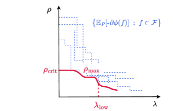
Figure 2: A central object of our analysis: the maximal radius $\rho_{\max}$, defined from the lower envelope of derivatives of $\phi$.

$$\rho_{\max}(\lambda)=\inf_{f\in\mathcal{F}}\mathbb{E}_{\xi\sim P}[-\partial_{\lambda}^{+}\phi(\lambda,f,\xi)].$$ (16)

As illustrated by Figure 2, $\rho_{\max}$ reaches its highest value at zero. This is the critical radius,

$$\rho_{\operatorname{crit}}=\rho_{\max}(0).$$

This particular quantity will be discussed in Section 5.2. As a central result of this work, we show that $\rho_{\max}$ can be made arbitrarily close to $\rho_{\operatorname{crit}}$ as $\lambda\to 0^{+}$.

Lemma 4.2.

$\lim_{\lambda\to 0^{+}}\rho_{\max}(\lambda)=\rho_{\operatorname{crit}}$. In particular, there exists $\lambda_{\operatorname{low}}>0$ such that for all $\lambda\in[0,2\lambda_{\operatorname{low}}]$, for all $f\in\mathcal{F}$,

$$\mathbb{E}_{\xi\sim P}[\partial^{+}_{\lambda}\phi(\lambda,f,\xi)]\leq-\frac{\rho_{\operatorname{crit}}}{2}.$$ (17)

Proof.

See Lemma D.1 in the supplementary. ∎

This means that the derivative condition (15) is satisfied whenever $\rho\leq\frac{\rho_{\operatorname{crit}}}{2}$. In order to transpose the inequality (17) to the empirical problem, precisely to obtain $\mathbb{E}_{\xi\sim\widehat{P}_{n}}[\partial^{+}_{\lambda}\phi(\lambda,f,\xi)]\leq-\frac{\rho_{\operatorname{crit}}}{2}$ with high probability, we would like to apply the concentration theorem (Theorem 4.1). Unfortunately, the derivative $\partial^{+}_{\lambda}\phi(\lambda,\cdot,\xi)$ is discontinuous and doesn’t satisfy the Lipschitz condition (ii) from Theorem 4.1. Indeed, its expression is inherently given by the envelope formula (Theorem 2.8.2, [14]) involving an arg max:

$$\partial^{+}_{\lambda}\phi(\lambda,f,\xi)=-\min_{\zeta\in\Xi}\{c(\zeta,\operatorname*{arg\,max}_{\Xi}\left\{f-\lambda c(\xi,\cdot)\right\}\}.$$

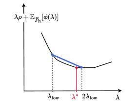
Figure 3: Bounding from below the empirical dual solution $\lambda^{*}$ expresses as a slope condition (thanks to convexity of the objective).

Dual bound on the empirical risk.

We propose a simple way to overcome the limitation highlighted above by relying on the convexity of $\phi$. Indeed, given a convex function $g$ over $\mathbb{R}^{+}$, the infimum of $g$ has to occur on an interval $[\lambda_{\operatorname{low}},+\infty]$ if $g$ has a negative slope between $\lambda_{\operatorname{low}}$ and $2\lambda_{\operatorname{low}}$ (Figure 3):

$$\frac{g(2\lambda_{\operatorname{low}})-g(\lambda_{\operatorname{low}})}{\lambda_{\operatorname{low}}}\leq 0\implies\inf_{\lambda\geq\lambda_{\operatorname{low}}}g(\lambda)=\inf_{\lambda\geq 0}g(\lambda).$$

We want this condition satisfied for the empirical Lagrangian function $g(\lambda)=\lambda\rho+\mathbb{E}_{\widehat{P}_{n}}[\phi(\lambda,f)]$ with high probability. For convenience, this can be expressed with the slope of $\mathbb{E}_{\widehat{P}_{n}}[\phi(\cdot,f)]$:

$$\widehat{s}(f)\!:=\!\frac{\mathbb{E}_{\widehat{P}_{n}}[\phi(2\lambda_{\operatorname{low}},f)]-\mathbb{E}_{\widehat{P}_{n}}[\phi(\lambda_{\operatorname{low}},f)]}{\lambda_{\operatorname{low}}}\leq-\rho.$$ (18)

This is the condition we aim to obtain. To this end, we proceed by comparing the empirical slope to the true one,

$$s(f):=\frac{\mathbb{E}_{P}[\phi(2\lambda_{\operatorname{low}},f)]-\mathbb{E}_{P}[\phi(\lambda_{\operatorname{low}},f)]}{\lambda_{\operatorname{low}}}.$$

Indeed, we can show that any function $(f,\xi)\mapsto\phi(\lambda,f,\xi)$, with $\lambda\in\mathbb{R}_{+}$, satisfies the requirements for the concentration theorem (Theorem 4.1):

Lemma 4.3.

For almost all $\xi\in\Xi$ we have

1. For all $\lambda\geq 0$ and $f\in\mathcal{F}$,

   $$\phi(\lambda,f,\xi)\in[-\|\mathcal{F}\|_{\infty},\|\mathcal{F}\|_{\infty}].$$

2. For all $\lambda\geq 0$, $f\mapsto\phi(\lambda,f,\xi)$ is Lipschitz continuous on $\mathcal{F}$ with constant $1$.

Proof.

See Lemma C.1.1. ∎

Consequently, we can apply the concentration theorem twice, on each function $\phi(2\lambda_{\operatorname{low}},\cdot,\cdot)$ and $\phi(2\lambda_{\operatorname{low}},\cdot,\cdot)$, to obtain that $\widehat{s}(f)$ approximates $s(f)$ with high probability, up to a term of the form $\frac{\beta}{\sqrt{n}}$:

$$\forall f\in\mathcal{F},\quad\widehat{s}(f)\leq s(f)+\frac{\beta}{\sqrt{n}}.$$

On the other hand, $s(f)\leq\mathbb{E}_{P}[\partial^{+}_{\lambda}\phi(2\lambda_{\operatorname{low}},f)]$ by convexity of $\phi$, hence $s(f)\leq-\frac{\rho_{\operatorname{crit}}}{2}$ by (17). This means

$$\widehat{s}(f)\leq\frac{\beta}{\sqrt{n}}-\frac{\rho_{\operatorname{crit}}}{2},$$

hence we have the desired condition (18) when

$$\rho<\frac{\rho_{\operatorname{crit}}}{2}-\frac{\beta}{\sqrt{n}}.$$

4.5 Extension to (double) regularization.

The strategy of Section 4.2 is flexible enough to be extended to the regularized setting of Section 3.2. Indeed, the regularized problem also has a dual representation, with a dual generator defined by

$$\phi^{\tau,\epsilon}(\lambda,f,\xi)=(\epsilon+\lambda\tau)\log\mathbb{E}_{\zeta\sim\pi_{0}(\cdot|\xi)}\left[e^{\frac{f(\zeta)-\lambda c(\xi,\zeta)}{\epsilon+\lambda\tau}}\right],$$

where $\epsilon>0$ and $\tau\geq 0$. Strong duality has been shown in [6]. We explain in Appendix B, Proposition B.2 how it applies to our general setting. This regularized dual generator leads to smooth counterparts of the key nonsmooth functions $\psi$, $\rho_{\max}$ and $\rho_{\operatorname{crit}}$ of the proof. In particular, we can show the regularized version of Lemma 4.2.

Lemma 4.4.

$\lim_{\lambda\to 0^{+}}\rho_{\max}^{\tau,\epsilon}(\lambda)=\rho_{\operatorname{crit}}^{\tau,\epsilon}$. In particular, there exists $\lambda_{\operatorname{low}}^{\tau,\epsilon}>0$ such that for all $\lambda\in[0,2\lambda_{\operatorname{low}}^{\tau,\epsilon}]$, $\forall f\in\mathcal{F}$,

$$\mathbb{E}_{\xi\sim P}[\partial_{\lambda}\phi^{\tau,\epsilon}(\lambda,f,\xi)]\leq-\frac{\rho_{\operatorname{crit}}^{\tau,\epsilon}}{2}.$$

Then we obtain Theorem 3.2 by repeating the proof scheme ofSection 4.2. The core results that simultaneously lead to Theorems 3.1 and 3.2 are gathered in Section E.1. Due to the smoothness of $\rho_{\max}^{\tau,\epsilon}$, an expression of $\lambda_{\operatorname{low}}^{\tau,\epsilon}$ can also be obtained; see Lemma D.2.

The key difference brought by regularization is that the Lipschitz property of $\psi^{\tau,\epsilon}$ is lost when $\mu\to 0$. This is an inherent peculiarity of the regularized setting which may occur over the whole family $\mathcal{F}$ and the space $\Xi$; see the example of Proposition F.2. This prevents to use the concentration result without guaranteeing that we can set a lower bound on $\mu$ or equivalently an upper-bound on $\lambda$. This is the purpose of the next lemma which establishes the existence of such an upper-bound, for any distribution.

Lemma 4.5.

Let $Q\in\mathcal{P}(\Xi)$ and $\lambda_{\operatorname{up}}:=\frac{2\|\mathcal{F}\|_{\infty}}{\rho-m_{c}}$. Then for all $f\in\mathcal{F}$,

$$R_{\rho,Q}(f)=\inf_{\lambda\in[0,\lambda_{\operatorname{up}}]}\left\{\lambda\rho+\mathbb{E}_{\xi\sim Q}[\phi(\lambda,f,\xi)]\right\}.$$

Proof.

See Lemma D.3 in the supplementary. ∎

5 On the generalization constants

In this section, we put our generalization results into perspective by further discussing the bounds $\alpha,\beta$, the critical radius $\rho_{\operatorname{crit}}$ appearing in Theorem 3.1, as well as their regularized counterparts of Theorem 3.2.

5.1 Sample complexity

We give the complete expressions of $\alpha$, $\beta$, $\alpha^{\tau,\epsilon}$ and $\beta^{\tau,\epsilon}$ in the detailed versions of Theorems 3.1 and 3.2 in Section E.2. Here we highlight their dependence from the problem’s constants.

First, in the setting of Theorem 3.1, $\alpha$ and $\beta$ grow essentially with the size and the complexity of $\mathcal{F}$. Indeed, we have

$$\alpha =O\big{(}\mathcal{I}(\mathcal{F},\|\cdot\|_{\infty})\times\|\mathcal{F}\|_{\infty}\big{)},$$ (19)

$$\beta =O\big{(}\|\mathcal{F}\|_{\infty}+\mathcal{I}(\mathcal{F},\|\cdot\|_{\infty})\big{)}.$$

The Dudley’s entropy $\mathcal{I}(\mathcal{F},\|\cdot\|_{\infty})$ quantifies the complexity of $\mathcal{F}$. In the large class of Lipschitz functions, this quantity is exponential in the data dimension. In practice, most machine learning problems involve a Lipschitz parametric family of losses (Section 2) in which case $\mathcal{I}(\mathcal{F},\|\cdot\|_{\infty})$ becomes proportional to $\sqrt{p}$, where $p$ is the parameter’s dimension (see e.g. Chapter 5.1 from [37]).

The constants $\alpha$ and $\beta$ also grow with $1/\lambda_{\operatorname{low}}$ and we have $\alpha=O\left(1/{\lambda_{\operatorname{low}}^{2}}\right)$ and $\beta=O\left(1/{\lambda_{\operatorname{low}}}\right)$. The constant ${\lambda_{\operatorname{low}}}$ is implicitly defined and depends on the regularity at $0$ of $\rho_{\max}$ (16), hence it may depend on $\mathcal{F}$, $\Xi$, $c$ and $P$.

In the setting of Theorem 3.2, we have similar interpretations. In addition to the conditional moment $m_{c}$ (9), the constants $\alpha^{\tau,\epsilon}$ and $\beta^{\tau,\epsilon}$ also involve the second order conditional moment:

$$m_{2,c}=\max_{\xi\in\Xi}\mathbb{E}_{\zeta\sim\pi_{0}(\cdot|\xi)}[c(\xi,\zeta)^{2}].$$

They are parameters that may be chosen in practice and related to the reference coupling $\pi_{0}$. For instance, if $\pi_{0}(\cdot|\xi)$ is a truncated Gaussian $\pi_{0}(\cdot|\xi)\propto e^{-\frac{\|\cdot-\xi\|^{2}}{2\sigma^{2}}}\mathds{1}_{\Xi}$ and $c(\xi,\zeta)=\frac{1}{2}\|\xi-\zeta\|^{2}$ we have $m_{c}\propto\sigma^{2}$ and $m_{2,c}\propto\sigma^{4}$.

The coefficients $\alpha^{\tau,\epsilon}$ and $\beta^{\tau,\epsilon}$ exhibit similar relations with $\lambda_{\operatorname{low}}^{\tau,\epsilon}$, $\|\mathcal{F}\|_{\infty}$, and $\mathcal{I}(\mathcal{F},\|\cdot\|_{\infty})$ to their counterparts $\alpha$ and $\beta$ (19). Regarding the hyperparameters $m_{c}$, $\epsilon$, $\tau$ and $\rho$, they should be of comparable order according to the expression of $\alpha^{\tau,\epsilon}$ (Theorem E.2). Compared to the standard setting, we have an estimate of the lower bound $\lambda_{\operatorname{low}}^{\tau,\epsilon}$ (Lemma D.2) showing dependence on the loss family: $1/{\lambda_{\operatorname{low}}^{\tau,\epsilon}}=O\big{(}e^{\frac{\|\mathcal{F}\|_{\infty}}{\epsilon}}\big{)}$.

5.2 The critical radius

In the standard setting, the critical radius has the expression

$$\rho_{\operatorname{crit}}=\mathbb{E}_{\xi\sim P}\left[\min\left\{c(\xi,\zeta)\ :\ \zeta\in\operatorname*{arg\,max}_{\Xi}f\right\}\right].$$

Assuming $\rho_{\operatorname{crit}}>0$ excludes losses that remain constant across all samples from the ground truth distribution $P$. This assumption reasonably aligns with practice and appeared in previous works [3, 5]. For instance, obtaining a predictor that precisely interpolates the ground truth distribution (leading to a loss equal to zero everywhere) is unrealistic. It also defines a threshold to exclude degenerated problems: if $\rho>\rho_{\operatorname{crit}}$, then there exists $f\in\mathcal{F}$ such that $R_{\rho}(f)=\max_{\Xi}f$ and the problem becomes independent from $\rho$, see [5].

A similar interpretation can be made in the regularized case with smoothed counterparts. Indeed, we can verify that if $\rho>\rho_{\operatorname{crit}}^{\tau,\epsilon}$, then there exists $f\in\mathcal{F}$ such that

$$R^{\tau,\epsilon}_{\rho}(f)=\sup_{\begin{subarray}{c}\pi\in\mathcal{P}(\Xi\times\Xi),[\pi]_{1}=P\end{subarray}}\left\{\mathbb{E}_{[\pi]_{2}}[f]-\operatorname{KL}(\pi\|\pi_{0})\right\},$$

and the problem becomes independent from $\rho$, see in particular Proposition F.1 in the supplementary.

6 Conclusion

In this work, we provide exact generalization guarantees of (regularized) Wasserstein robust models, covering all usual machine learning situations, without restrictive assumptions (on the Wasserstein metric or the class of functions). We achieve these universal results by directly addressing the intrinsic nonsmoothness of robust problems. Our results thus give users freedom when choosing the radius $\rho$: for all usual situations, it is not necessary to consider specific regimes for $\rho$ in order to expect good generalization from robust models. Further research can now focus on practical aspects: it would be of premier interest to design efficient practical procedures for selecting $\rho$, and more generally, scalable algorithms for solving distributionally robust optimization problems.

Supplementary Material

This supplementary gathers recalls, technical results, and examples, as well as, the detailed proof of the results of the main text. The core of our contributions are presented in Appendices D and E. The whole supplementary is organized as follows:

- In Appendix A, we recall some essential mathematical tools. They include a uniform concentration inequality (Theorem A.2), continuity notions in nonsmooth analysis, and the envelope formula to differentiate supremum functions (Theorem A.1).

- In Appendix B, we present strong duality results for WDRO and its regularized version. We explain in particular how the duality theorem from [6] can be easily adapted to our setting.

- Appendix C contains preliminary computations in view of applying the uniform concentration theorem.

- In Appendix D, we demonstrate the existence of a dual lower bound in the standard and regularized cases. In particular, the proofs involve the maximal radius introduced in Section 4.4.

- By using these preliminary results, in Appendix E, we prove our main generalization theorems (Theorem 3.1 and 3.2). Detailed versions with constants’ expressions are proved, Theorem E.1 for the standard setting, and Theorem E.2 for the regularized setting.

- Appendix F contains minor results supporting several remarks found in the article. They include the interpretation of the critical radius in the regularized case, a counter-example justifying the upper-bound in the regularized case and the interpretation of the restrictive compactness assumptions used in [5].

Notations

Throughout the proofs will use the following notations:

In Wasserstein robust models:

• $\phi(\lambda,f,\xi)=\sup_{\zeta\in\Xi}\left\{f(\zeta)-\lambda c(\xi,\zeta)\right\}$

• $\psi(\mu,f,\xi)=\mu\phi(\mu^{-1},f,\xi)$

In Wasserstein robust models with double regularization:

• $\phi^{\tau,\epsilon}(\lambda,f,\xi)=(\epsilon+\lambda\tau)\log\mathbb{E}_{\zeta\sim\pi_{0}(\cdot|\xi)}\left[e^{\frac{f(\zeta)-\lambda c(\xi,\zeta)}{\epsilon+\lambda\tau}}\right]$

• $\psi^{\tau,\epsilon}(\mu,f,\xi)=\mu\phi^{\tau,\epsilon}(\mu^{-1},f,\xi)$

Given a measurable function $h:\Xi\to\mathbb{R}$ and $\pi\in\mathcal{P}(\Xi)$ the Gibbs distribution $\pi^{h}$ is defined as

$$\mathrm{d}\pi^{h}\propto e^{h}\mathrm{d}\pi.$$

Appendix A Recalls and technical preliminaries

In this part, we use the notation $G:\mathcal{X}\rightrightarrows\mathcal{Y}$ to denote a function $G$ defined on $\mathcal{X}$ and valued in the set of subsets of $\mathcal{Y}$.

Semicontinuity notions will be necessary to understand the proof of Lemma D.1. They are regularity notions recurrently arising when manipulating nonsmooth convex functions.

Definition A.1 (Lower and upper semicontinuity, 2.42 in [1]).

Let $(\mathcal{X},\operatorname{dist})$ be a metric space and let $f:\mathcal{X}\to\mathbb{R}$. Then

1. $f$ is called lower semicontinuous if for all $x\in\mathcal{X}$, $\liminf_{y\to x}f(y)\geq f(x)$.

2. $f$ is called upper semicontinuous if for all $x\in\mathcal{X}$, $\limsup_{y\to x}f(y)\leq f(x)$.

In particular, if $f$ is lower semicontinuous, then $-f$ is upper semicontinuous.

Outer semicontinuity can be seen as the set-valued counterpart of upper semicontinuity:

Definition A.2 (Outer semicontinuity).

Let $\mathcal{X}$ and $\mathcal{Y}$ two metric spaces. Then a measurable and compact-valued map $G:\mathcal{X}\rightrightarrows\mathcal{Y}$ is called outer semicontinuous at $x\in\mathcal{X}$ if for all open subset $V\subset\mathcal{Y}$ containing $G(x)$, there exists a neighborhood $U$ of $x$ which is such that for all $w\in U$, $G(w)\subset V$.

Semicontinuity of maximum and $\operatorname*{arg\,max}$ functions are central to the proof of Lemma D.1:

Lemma A.1 (17.30 in [1]).

Let $\mathcal{X}$ and $\Xi$ be two metric spaces and let $G:\mathcal{X}\rightrightarrows\Xi$ be outer semicontinuous with nonempty compact values, $h:\Xi\times\Xi\rightarrow\mathbb{R}$ continuous. Then the function

$$x\mapsto\max\{h(x,v)\ :\ v\in G(x)\}$$

is upper semicontinuous. In particular, $u\mapsto\min\{h(u,v)\ :\ v\in G(x)\}$ is lower semicontinuous.

Lemma A.2 (17.31 in [1]).

If $\mathcal{X}$ is a metric space, $(\Xi,d)$ is a compact metric space, and $h:\mathcal{X}\times\Xi\to\mathbb{R}$ is continuous, then the function $x\mapsto\max_{z\in\Xi}h(x,z)$ is continuous, and the set-valued map $x\mapsto\operatorname*{arg\,max}_{z\in\Xi}h(x,z)$ is outer semicontinuous.

We recall the definition of gradient for a nonsmooth convex function. This the subdifferential.

Definition A.3 (Subdifferential of convex function).

Let $\phi:\mathbb{R}^{m}\to\mathbb{R}$ be a convex function. Then we call subdifferential of $\phi$ the set-valued map $\partial\phi:\mathbb{R}^{m}\rightrightarrows\mathbb{R}^{m}$ such that for all $x\in\mathbb{R}^{m}$ and $y\in\mathbb{R}^{m}$,

$$\phi(y)\geq\phi(x)+\langle v,y-x\rangle\text{ for all }v\in\partial\phi(x).$$

In particular, we may apply the envelope formula to compute the subdifferential of a maximum function:

Theorem A.1 (Envelope formula, Corollary 1, Chapter 2.8 in [14]).

Let $(\Xi,d)$ be a compact metric space and $g:\mathbb{R}^{m}\times\Xi\to\mathbb{R}$ such that

1. For all $x\in\mathbb{R}^{m}$, $g(x,\cdot)$ is continuous.

2. For all $\zeta\in\Xi$, $g(\cdot,\zeta)$ is convex with subdifferential $\partial_{x}g(\cdot,\zeta)$.

Then $G:=\sup_{\zeta\in\Xi}g(\cdot,\zeta)$ is convex on $\mathbb{R}^{m}$, and its subdifferential is given for all $x\in\mathbb{R}^{m}$ by

$$\partial G(x):=\operatorname{conv}\{v\ :\ v\in\partial_{x}g(x,\zeta),\,\zeta\in\operatorname*{arg\,max}_{\Xi}g(x,\cdot)\}.$$

where $\operatorname{conv}$ denotes the convex hull of a set.

A.1 Uniform concentration inequality

We recall a concentration inequality that gives a high probability uniform bound for a family of bounded and Lipschitz functions. This is an extended version of Theorem 4.1 which details the one-sided inequalities (without the absolute value). We refer the reader to [12] for a complete reference on concentration inequalities, and Lemma G.2 in [5] for the proof of such a result.

Theorem A.2 (Uniform concentration inequality, Lemma G.2 in [5]).

Let $(\mathcal{X},\text{dist})$ be a (totally bounded) separable metric space, $P$ a probability distribution on a probability space $\Xi$, and $\widehat{P}_{n}=\frac{1}{n}\sum_{i=1}^{n}\delta_{\xi_{i}}$ with $\xi_{1},\ldots,\xi_{n}\overset{\text{i.i.d.}}{\sim}P$. Consider a measurable mapping $X:\mathcal{X}\times\Xi\rightarrow\mathbb{R}$ and assume that,

1. There is a constant $L>0$ such that, for each $\xi\in\Xi$, $x\mapsto X(x,\xi)$ is $L$-Lipschitz.

2. $X(\cdot,\xi)$ almost surely belongs to $[a,b]$.

Then, for any $\delta\in(0,1)$, we respectively have

1. With probability at least $1-\delta$,

   $$\sup_{x\in\mathcal{X}}\left\{\mathbb{E}_{\xi\sim\widehat{P}_{n}}[X(x,\xi)]-\mathbb{E}_{\xi\sim P}[X(x,\xi)]\right\}\leq\frac{48L\mathcal{I(\mathcal{X,\operatorname{dist}})}}{\sqrt{n}}+(b-a)\sqrt{2\frac{\log\frac{1}{\delta}}{n}}.$$

2. With probability at least $1-\delta$,

   $$\sup_{x\in\mathcal{X}}\left\{\mathbb{E}_{\xi\sim P}[X(x,\xi)]-\mathbb{E}_{\xi\sim\widehat{P}_{n}}[X(x,\xi)]\right\}\leq\frac{48L\mathcal{I(\mathcal{X,\operatorname{dist}})}}{\sqrt{n}}+(b-a)\sqrt{2\frac{\log\frac{1}{\delta}}{n}}.$$

The quantity $\mathcal{I}(\mathcal{X},\operatorname{dist})$ is defined as follows:

Definition A.4.

Given a compact metric space $(\mathcal{X},\operatorname{dist})$, Dudley’s entropy integral, $\mathcal{I}(\mathcal{X},\operatorname{dist})$, is defined as

$$\mathcal{I}(\mathcal{X},\operatorname{dist}):=\int_{0}^{\infty}\sqrt{\log N(t,\mathcal{X},\operatorname{dist})}dt$$

where $N(t,\mathcal{X},\text{dist})$ denotes the $t$-packing number of $\mathcal{X}$, which is the maximal number of points in $\mathcal{X}$ that are at least at a distance $t$ from each other.

We may recall some properties of Dudley’s entropy for Cartesian products and segments from $\mathbb{R}$. These are known results, see e.g. [37] and Lemmas G.3 and G.4 from [5] for proofs.

Lemma A.3 (Dudley’s integral estimates).

2. (on Cartesian products) Let $(\mathcal{X}_{1},\operatorname{dist}_{1})$ and $(\mathcal{X}_{2},\operatorname{dist}_{2})$ be two metric spaces. Consider the product space $\mathcal{X}:=\mathcal{X}_{1}\times\mathcal{X}_{2}$ equipped with the distance $\operatorname{dist}:=\operatorname{dist}_{1}+\operatorname{dist}_{2}$. Then we have the inequality

   $$\mathcal{I}(\mathcal{X},\operatorname{dist})\leq\mathcal{I}(\mathcal{X}_{1},\operatorname{dist}_{1})+\mathcal{I}(\mathcal{X}_{2},\operatorname{dist}_{2}).$$

3. (on $\mathbb{R}$) Let $c>0$. Then we have the inequality

   $$\mathcal{I}([0,c],|\cdot|)\leq\frac{3c}{2}.$$

Appendix B Strong duality

In this section, we recall duality results for WDRO [8] and its regularized version [6]. We recall the Wasserstein distance with cost $c$ for $(Q,Q^{\prime})\in\mathcal{P}(\Xi)\times\mathcal{P}(\Xi)$:

$$W_{c}(Q,Q^{\prime})=\inf\left\{\mathbb{E}_{(\xi,\zeta)\sim\pi}[c(\xi,\zeta)]\ :\ \pi\in\mathcal{P}(\Xi\times\Xi),[\pi]_{1}=Q,[\pi]_{2}=Q^{\prime}\right\}.$$

Proposition B.1 (Strong duality, standard WDRO).

Under 2.1, for any $Q\in\mathcal{P}(\Xi)$ and $\rho>0$,

$$\max_{W_{c}(Q,Q^{\prime})\leq\rho}\mathbb{E}_{\xi\sim Q^{\prime}}[f(\xi)]=\inf_{\lambda\geq 0}\left\{\lambda\rho+\mathbb{E}_{\xi\sim Q}[\phi(\lambda,f,\xi)]\right\}.$$

Proof.

This is an application of Theorem 1 from [8]. In particular, Assumptions 1 and 2 from [8] are satisfied through 2.1. ∎

Proposition B.2 (Strong duality, regularized WDRO).

Under 2.1, for any $Q\in\mathcal{P}(\Xi)$ and $\rho>0$,

$$\max_{\begin{subarray}{c}\pi\in\mathcal{P}(\Xi\times\Xi)\\ [\pi]_{1}=Q\\ \mathbb{E}_{\pi}[c]+\tau\operatorname{KL}(\pi\|\pi_{0})\leq\rho\end{subarray}}\left\{\mathbb{E}_{\xi\sim[\pi]_{2}}[f(\zeta)]-\epsilon\operatorname{KL}(\pi\|\pi_{0})\right\}=\inf_{\lambda\geq 0}\left\{\lambda\rho+\mathbb{E}_{\xi\sim Q}[\phi^{\tau,\epsilon}(\lambda,f,\xi)]\right\}.$$

Proof.

This is an application of Theorem 3.1 from [6], which is a corollary to Theorem 2.1 [6]. Note that the proofs of Theorems 2.1 and 3.1 from [6] can be easily extended to a general compact metric space $(\Xi,d)$, without being rewritten entirely. Precisely, only two arguments in their proofs rely on the real-valued setting [31] but can be directly extended to a general metric space as follows:

• In the proof of Theorem 2.1 from [6], one needs to justify

  $$\sup\left\{\mathbb{E}_{\xi\sim P}\left[\varphi(\xi,\zeta(\xi))\right]\ :\ \zeta:\Xi\to\Xi\text{ measurable}\right\}\geq\mathbb{E}_{\xi\sim P}\left[\sup_{\zeta\in\Xi}\varphi(\xi,\zeta)\right].$$ (20)

  To this end, the authors use the notion of normal integrand from [31]. Actually, (20) holds true in a compact metric space: if $\varphi$ is continuous, then by compactness of $\Xi$, the set-valued map $\xi\mapsto\operatorname*{arg\,max}_{\zeta\in\Xi}\varphi(\xi,\zeta)$ admits a measurable selection $\zeta^{*}$, by the measurable maximum theorem, see 18.19 in [1]. Such a selection $\zeta^{*}$ then satisfies $\varphi(\xi,\zeta^{*}(\xi))=\sup_{\zeta\in\Xi}\varphi(\xi,\zeta)$ for all $\xi\in\Xi$, hence the result.

• In the proof of Theorem 3.1 from [6], $g^{\varphi}=\sup_{\zeta\in\Xi}\varphi(\cdot,\zeta)$ is actually continuous by Lemma A.2 and the approximation by the infimal convolutions $(g_{k}^{\varphi})_{k\in\mathbb{N}}$ need not be done.

Note also that the convexity of $\Xi$ is not required in this proof (although stated in Assumption 1 from [6]). ∎

Appendix C Concentration constants

In this part, we compute several constants in view of applying Theorem A.2 for the main proofs of Appendix E.

C.1 Standard WDRO

The following lemma gathers Lemma 4.1 and Lemma 4.3. We compute bounds (i) and global Lipschitz constants (ii) for $\phi$ and $\psi$.

Lemma C.1 (Concentration conditions for WDRO).

we have the following:

1. 1. For all $\lambda\geq 0$, $f\in\mathcal{F}$ and $\xi\in\Xi$, $\phi(\lambda,f,\xi)\in[-\|\mathcal{F}\|_{\infty},\|\mathcal{F}\|_{\infty}].$

   2. For all $\lambda\geq 0$ and $\xi\in\Xi$, $f\mapsto\phi(\lambda,f,\xi)$ is Lipschitz continuous on $\mathcal{F}$ with constant $1$.

2. 1. Given $\lambda_{\operatorname{low}}>0$, for all $\mu\in(0,\lambda_{\operatorname{low}}^{-1}]$ and $f\in\mathcal{F}$, $\psi(\mu,f,\xi)\in\left[-\frac{\|\mathcal{F}\|_{\infty}}{\lambda_{\operatorname{low}}},\frac{\|\mathcal{F}\|_{\infty}}{\lambda_{\operatorname{low}}}\right]$.

   2. For all $\xi\in\Xi$, $(\mu,f)\mapsto\psi(\mu,f,\xi)$ is Lipschitz continuous on $(0,\lambda_{\operatorname{low}}^{-1}]$ with constant $\|\mathcal{F}\|_{\infty}+\lambda_{\operatorname{low}}^{-1}$.

Proof.

1. (i) Let $(\lambda,f,\xi)\in\mathbb{R}_{+}\times\mathcal{F}\times\Xi$. Recall that $\phi(\lambda,f,\xi):=\sup_{\zeta\in\Xi}\left\{f(\zeta)-\lambda c(\xi,\zeta)\right\}$. Since $c$ is nonnegative, we have $\phi(\lambda,f,\xi)\leq\|\mathcal{F}\|_{\infty}$. On the other hand, since $c(\xi,\xi)=0$, we also have $\phi(\lambda,f,\xi)\geq f(\xi)\geq-\|\mathcal{F}\|_{\infty}$. Finally, we have $\phi(\lambda,f,\xi)\in[-\|\mathcal{F}\|_{\infty},\|\mathcal{F}\|_{\infty}]$.

(ii) Let $\lambda\geq 0$, $\xi\in\Xi$ and $(f,f^{\prime})\in\mathcal{F}\times\mathcal{F}$. For all $\zeta\in\Xi$, we have

$$f(\zeta)-\lambda c(\xi,\zeta)-\phi(\lambda,f^{\prime},\xi) \leq f(\zeta)-\lambda c(\xi,\zeta)-(f^{\prime}(\zeta)-\lambda c(\xi,\zeta))$$

$$\leq f(\zeta)-f^{\prime}(\zeta)$$

$$\leq\|f-f^{\prime}\|_{\infty}.$$

Taking the supremum over $\zeta\in\Xi$ on the left-hand side gives $\phi(\lambda,f,\xi)-\phi(\lambda,f^{\prime},\xi)\leq\|f-f^{\prime}\|_{\infty}$. Permuting the roles of $f$ and $f^{\prime}$ yields $|\phi(\lambda,f,\xi)-\phi(\lambda,f^{\prime},\xi)|\leq\|f-f^{\prime}\|_{\infty}$. We proved that $\phi(\lambda,\cdot,\xi)$ is $1$-Lipschitz continuous.

2. (i) Now, let $\lambda_{\operatorname{low}}>0$ and let $(\mu,f,\xi)\in(0,\lambda_{\operatorname{low}}^{-1}]\times\mathcal{F}\times\Xi$ be arbitrary. Then we have

$$\mu\phi(\mu^{-1},f,\xi)=\sup_{\zeta\in\Xi}\left\{\mu f(\zeta)-c(\xi,\zeta)\right\}\leq\frac{\|\mathcal{F}\|_{\infty}}{\lambda_{\operatorname{low}}}.$$

On the other hand, using $c(\xi,\xi)=0$ we obtain

$$\sup_{\zeta\in\Xi}\left\{\mu f(\zeta)-c(\xi,\zeta)\right\}\geq\mu f(\xi)\geq-\frac{\|\mathcal{F}\|_{\infty}}{\lambda_{\operatorname{low}}},$$

whence we have $\mu\phi(\mu^{-1},f,\xi)\in\left[-\frac{\|\mathcal{F}\|_{\infty}}{\lambda_{\operatorname{low}}},\frac{\|\mathcal{F}\|_{\infty}}{\lambda_{\operatorname{low}}}\right]$.

(ii) Toward a proof of 2. (ii), let $\lambda_{\operatorname{low}}>0$, and $\xi\in\Xi$ and $\mu\in(0,\lambda_{\operatorname{low}}]$. Remark that $\mu\phi(\mu^{-1},f,\xi)=\sup_{\zeta\in\Xi}\left\{\mu f(\zeta)-c(\xi,\zeta)\right\}$. The function $(\mu,f)\mapsto\mu\phi(\mu^{-1},f,\xi)$ write as a composition $u\circ v$ where $u(h):=\sup_{\zeta\in\Xi}\left\{h(\zeta)-c(\xi,\zeta)\right\}$ for $h\in C(\Xi,\mathbb{R})$, and $v(\mu,f):=\mu f$ for $\mu\in(0,\lambda_{\operatorname{low}}^{-1}]$. $u$ is 1-Lipschitz continuous with respect to $\|\cdot\|_{\infty}$. As to $v$, we can write

$$\mu f-\mu^{\prime}f^{\prime}=\mu(f-f^{\prime})+f^{\prime}(\mu-\mu^{\prime}),$$

whence $v$ is clearly $(\|\mathcal{F}\|_{\infty}+\lambda_{\operatorname{low}}^{-1})$-Lipschitz continuous on $(0,\lambda_{\operatorname{low}}^{-1}]\times\mathcal{F}$. By composition, $u\circ v$ is Lipschitz continuous with constant $\|\mathcal{F}\|_{\infty}+\lambda_{\operatorname{low}}^{-1}$. ∎

C.2 Regularized WDRO

We will use the following lemma repeatedly:

Lemma C.2 (Lemma G.7 in [5]).

Let $g:\Xi\to\mathbb{R}$ be a measurable bounded function and $Q\in\mathcal{P}(\Xi)$. Then one has the inequality

$$\log\mathbb{E}_{\zeta\sim Q}\left[e^{g(\zeta)}\right]\leq\frac{\mathbb{E}_{\zeta\sim Q}[g(\zeta)e^{g(\zeta)}]}{\mathbb{E}_{\zeta\sim Q}[e^{g(\zeta)}]}.$$

We prove the regularized version of Lemma C.1:

Lemma C.3 (Concentration conditions for regularized WDRO).

Let $\xi\in\Xi$. Then

1. 1. For all $\lambda\geq 0$ and $f\in\mathcal{F}$, $\phi^{\tau,\epsilon}(\lambda,f,\xi)\in\left[-\|\mathcal{F}\|_{\infty}-\lambda m_{c},\|\mathcal{F}\|_{\infty}\right].$

   2. For all $\lambda\geq 0$, $f\mapsto\phi^{\tau,\epsilon}(\lambda,f,\xi)$ is Lipschitz continuous with constant $1$.

2. 1. Given $\lambda_{\operatorname{low}}>0$, for all $\mu\in[\lambda_{\operatorname{up}}^{-1},\lambda_{\operatorname{low}}^{-1}]$ and $f\in\mathcal{F}$, $\psi^{\tau,\epsilon}(\mu,f,\xi)\in\left[-\frac{\|\mathcal{F}\|_{\infty}}{\lambda_{\operatorname{low}}}-m_{c},\frac{\|\mathcal{F}\|_{\infty}}{\lambda_{\operatorname{low}}}\right].$

   2. Given $\lambda_{\operatorname{up}}>0$, $(\mu,f)\mapsto\psi^{\tau,\epsilon}(\mu,f,\xi)$ is Lipschitz continuous on $[\lambda_{\operatorname{up}}^{-1},\lambda_{\operatorname{low}}^{-1}]\times\mathcal{F}$ with constant $\|\mathcal{F}\|_{\infty}+\lambda_{\operatorname{low}}^{-1}+\left(\frac{\lambda_{\operatorname{up}}\epsilon}{\epsilon+\lambda_{\operatorname{up}}\tau}\right)m_{c}$.

Proof.

1. (i) Let $(\lambda,f,\xi)\in\mathbb{R}_{+}\times\mathcal{F}\times\Xi$. For all $\zeta\in\Xi$, $e^{\frac{f(\zeta)-\lambda c(\xi,\zeta)}{\epsilon+\lambda\tau}}\leq e^{\frac{\|\mathcal{F}\|_{\infty}}{\epsilon+\lambda\tau}}$. This gives

$$\phi^{\tau,\epsilon}(\lambda,f,\xi)\leq(\epsilon+\lambda\tau)\log\mathbb{E}_{\zeta\sim\pi_{0}(\cdot|\xi)}\left[e^{\frac{\|\mathcal{F}\|_{\infty}}{\epsilon+\lambda\tau}}\right]=\|\mathcal{F}\|_{\infty}.$$ (21)

On the other hand, $e^{\frac{f(\zeta)-\lambda c(\xi,\zeta)}{\epsilon+\lambda\tau}}\geq e^{\frac{-\|\mathcal{F}\|_{\infty}-\lambda c(\xi,\zeta)}{\epsilon+\lambda\tau}}$, which gives

$$\phi^{\tau,\epsilon}(\lambda,f,\xi) \geq(\epsilon+\lambda\tau)\log\left(e^{-\frac{\|\mathcal{F}\|_{\infty}}{\epsilon+\lambda\tau}}\mathbb{E}_{\zeta\sim\pi_{0}(\cdot|\xi)}\left[e^{-\frac{\lambda c(\xi,\zeta)}{\epsilon+\lambda\tau}}\right]\right)$$

$$\geq-\|\mathcal{F}\|_{\infty}+(\epsilon+\lambda\tau)\log\mathbb{E}_{\zeta\sim\pi_{0}(\cdot|\xi)}\left[e^{-\frac{\lambda c(\xi,\zeta)}{\epsilon+\lambda\tau}}\right]$$

$$\geq-\|\mathcal{F}\|_{\infty}-\lambda m_{c},$$ (22)

where for the last inequality we used Jensen’s inequality on the convex function $s\mapsto e^{-\frac{\lambda s}{\epsilon+\lambda\tau}}$.

Combining (21) and (C.2) gives

$$\phi^{\tau,\epsilon}(\lambda,f,\xi)\in[-\|\mathcal{F}\|_{\infty}-\lambda m_{c},\|\mathcal{F}\|_{\infty}].$$

(ii) Let $\xi\in\Xi$ and $\lambda\geq 0$. To compute the Lipschitz constant of $f\mapsto\phi^{\tau,\epsilon}(\lambda,f,\xi)$, we compute the derivative of $h_{v}:t\mapsto\phi^{\tau,\epsilon}(\lambda,f+tv,\xi)$ where $t\in\mathbb{R}$ and for an arbitrary direction $v\in\mathcal{F}$. We have

$$h_{v}(t)=(\epsilon+\lambda\tau)\log\mathbb{E}_{\zeta\sim\pi_{0}(\cdot|\xi)}\left[e^{\frac{f(\zeta)+tv(\zeta)-\lambda c(\xi,\zeta)}{\epsilon+\lambda\tau}}\right].$$

It is easy to verify that $h_{v}^{\prime}(t)=\mathbb{E}_{\zeta\sim\pi_{0}^{\frac{f+tv-\lambda c(\xi,\cdot)}{\epsilon+\lambda\tau}}(\cdot|\xi)}\left[v(\zeta)\right],$ whence $|h^{\prime}_{v}(t)|\leq\|v\|_{\infty}$. This means that $\phi^{\tau,\epsilon}(\lambda,\cdot,\xi)$ has Lipschitz constant $1$.

2. (i) Let $\lambda_{\operatorname{low}}>0$ and $(\mu,f,\xi)\in(0,\lambda_{\operatorname{low}}^{-1}]\times\mathcal{F}\times\Xi$. $\lambda$. We deduce from (21) and (C.2), with $\lambda=\mu^{-1}$, that

$$\mu\phi^{\tau,\epsilon}(\mu^{-1},f,\xi)\in\left[-\frac{\|\mathcal{F}\|_{\infty}}{\lambda_{\operatorname{low}}}-m_{c},\frac{\|\mathcal{F}\|_{\infty}}{\lambda_{\operatorname{low}}}\right].$$

(ii) Now, let $\xi\in\Xi$. Our goal is to compute a Lipschitz constant of $(\mu,f)\mapsto\mu\phi^{\tau,\epsilon}(\mu^{-1},f,\xi)$ on $[\lambda_{\operatorname{up}}^{-1},\lambda_{\operatorname{low}}^{-1}]\times\mathcal{F}$. We first compute a Lipschitz constant of

$$h_{f}:\mu\mapsto\mu\phi^{\tau,\epsilon}(\mu^{-1},f,\xi)=(\mu\epsilon+\tau)\log\mathbb{E}_{\zeta\sim\pi_{0}(\cdot|\xi)}\left[e^{\frac{\mu f(\zeta)-c(\xi,\zeta)}{\mu\epsilon+\tau}}\right]$$

on $[\lambda_{\operatorname{up}}^{-1},\lambda_{\operatorname{low}}^{-1}]$, for an arbitrary $f\in\mathcal{F}$. The derivative of $h_{f}$ is

$$h_{f}^{\prime}(\mu)=\frac{1}{\mu\epsilon+\tau}\frac{\mathbb{E}_{\zeta\sim\pi_{0}(\cdot|\xi)}\left[(\epsilon c(\xi,\zeta)+\tau f(\zeta))e^{\frac{\mu f(\zeta)-c(\xi,\zeta)}{\mu\epsilon+\tau}}\right]}{\mathbb{E}_{\zeta\sim\pi_{0}(\cdot|\xi)}\left[e^{\frac{\mu f(\zeta)-c(\xi,\zeta)}{\mu\epsilon+\tau}}\right]}+\epsilon\log\mathbb{E}_{\zeta\sim\pi_{0}(\cdot|\xi)}\left[e^{\frac{\mu f(\zeta)-c(\xi,\zeta)}{\mu\epsilon+\tau}}\right],$$

which we write

$$h_{f}^{\prime}(\mu)=\mathbb{E}_{\pi_{0}^{\frac{\mu f-c(\xi,\cdot)}{\mu\epsilon+\tau}}(\cdot|\xi)}\left[\frac{\epsilon c(\xi,\zeta)+\tau f(\zeta)}{\mu\epsilon+\tau}\right]+\epsilon\log\mathbb{E}_{\zeta\sim\pi_{0}(\cdot|\xi)}\left[e^{\frac{\mu f(\zeta)-c(\xi,\zeta)}{\mu\epsilon+\tau}}\right].$$ (23)

We bound $h^{\prime}_{f}(\mu)$ above. By Lemma C.2 with $Q=\pi_{0}(\cdot|\xi)$ and $g=\frac{\mu f-c(\xi,\cdot)}{\mu\epsilon+\tau}$, we have that

$$\epsilon\log\mathbb{E}_{\zeta\sim\pi_{0}(\cdot|\xi)}\left[e^{\frac{\mu f(\zeta)-c(\xi,\zeta)}{\mu\epsilon+\tau}}\right]\leq\mathbb{E}_{\zeta\sim\pi_{0}^{\frac{\mu f-c(\xi,\cdot)}{\mu\epsilon+\tau}}(\cdot|\xi)}\left[\frac{\epsilon\mu f(\zeta)-\epsilon c(\xi,\zeta)}{\mu\epsilon+\tau}\right]$$

which gives $h_{f}^{\prime}(\mu)\leq\mathbb{E}_{\zeta\sim\pi_{0}^{\frac{\mu f-c(\xi,\cdot)}{\mu\epsilon+\tau}}}[f(\zeta)]\leq\|\mathcal{F}\|_{\infty}$.

Now we bound $h_{f}^{\prime}(\mu)$ below. We start with the first term in (23). Since $c$ is nonnegative, we clearly have

$$\mathbb{E}_{\pi_{0}^{\frac{\mu f-c(\xi,\cdot)}{\mu\epsilon+\tau}}(\cdot|\xi)}\left[\frac{\epsilon c(\xi,\zeta)+\tau f(\zeta)}{\mu\epsilon+\tau}\right]\geq\frac{-\tau\|\mathcal{F}\|_{\infty}}{\mu\epsilon+\tau}$$ (24)

As to the second term of (23), we have by Jensen’s inequality,

$$\epsilon\log\mathbb{E}_{\zeta\sim\pi_{0}(\cdot|\xi)}\left[e^{\frac{\mu f(\zeta)-c(\xi,\zeta)}{\mu\epsilon+\tau}}\right]\geq-\frac{\epsilon\mu\|\mathcal{F}\|_{\infty}}{\mu\epsilon+\tau}-\frac{\epsilon m_{c}}{\mu\epsilon+\tau}$$ (25)

Combining (24) and (25) gives $h^{\prime}_{f}(\mu)\geq-\|\mathcal{F}\|_{\infty}-\frac{\lambda_{\operatorname{up}}\epsilon m_{c}}{\epsilon+\lambda_{\operatorname{up}}\tau}$. Finally, $h_{f}$ has Lipschitz constant $\|\mathcal{F}\|_{\infty}+\frac{\lambda_{\operatorname{up}}m_{c}}{\epsilon+\lambda_{\operatorname{up}}\tau}$

Since $\phi^{\tau,\epsilon}(\mu^{-1},\cdot,\xi)$ has Lipschitz constant $1$, then $\mu\leq\lambda_{\operatorname{low}}^{-1}$, the function $\mu\phi^{\tau,\epsilon}(\mu^{-1},\cdot,\xi)$ has Lipschitz constant $\lambda_{\operatorname{low}}^{-1}$.

Now, we can obtain a Lipschitz constant for

$$h:(\mu,f)\mapsto(\mu\epsilon+\tau)\log\mathbb{E}_{\zeta\sim\pi_{0}(\cdot|\xi)}\left[e^{\frac{\mu f(\zeta)-c(\xi,\zeta)}{\mu\epsilon+\tau}}\right]=\psi^{\tau,\epsilon}(\mu,f,\xi).$$

Indeed, for $(\mu,\mu^{\prime})\in[\lambda_{\operatorname{up}}^{-1},\lambda_{\operatorname{low}}^{-1}]\times[\lambda_{\operatorname{up}}^{-1},\lambda_{\operatorname{low}}^{-1}]$ and $(f,f^{\prime})\in\mathcal{F}\times\mathcal{F}$, we can write

$$|h(\mu,f)-h(\mu^{\prime},f^{\prime})| \leq|h(\mu,f)-h(\mu^{\prime},f)|+|h(\mu^{\prime},f)-h(\mu^{\prime},f^{\prime})|$$

$$\leq\left(\|\mathcal{F}\|_{\infty}+\left(\frac{\lambda_{\operatorname{up}}\epsilon}{\epsilon+\lambda_{\operatorname{up}}\tau}\right)\right)|\mu-\mu^{\prime}|+\lambda_{\operatorname{low}}^{-1}\|f-f^{\prime}\|_{\infty}.$$

hence $h$ has Lipschitz constant $\|\mathcal{F}\|_{\infty}+\lambda_{\operatorname{low}}^{-1}+\left(\frac{\lambda_{\operatorname{up}}\epsilon}{\epsilon+\lambda_{\operatorname{up}}\tau}\right)m_{c}$. ∎

Appendix D Dual bounds and maximal radius

We establish the existence of a dual lower bound on the true robust risk, for the standard WDRO problem in D.1 and for regularized WDRO in D.2. The proofs involve the maximal radius introduced in Section 4.4. For the regularized case, an estimate of the dual lower bound is provided.

D.1 Standard WDRO: continuity at zero of the maximal radius

For $\lambda\geq 0$, we consider the following quantities:

$$\rho_{\operatorname{crit}}=\inf_{f\in\mathcal{F}}\mathbb{E}_{\xi\sim P}[-\partial_{\lambda}^{+}\phi(0,f,\xi)]\qquad\rho_{\max}(\lambda)=\inf_{f\in\mathcal{F}}\mathbb{E}_{\xi\sim P}[-\partial_{\lambda}^{+}\phi(\lambda,f,\xi)].$$

Lemma D.1.

$\lim_{\lambda\to 0^{+}}\rho_{\max}(\lambda)=\rho_{\operatorname{crit}}.$

Proof.

For $\xi\in\Xi$, $f-\lambda c(\xi,\cdot)$ is continuous, hence we can apply the envelope formula (Theorem A.1) and the right-sided derivative of $\phi$ with respect to $\lambda$ is $\partial^{+}_{\lambda}\phi(\lambda,f,\xi)=-\min\left\{c(\xi,\zeta)\ :\ \zeta\in\operatorname*{arg\,max}_{\Xi}\left\{f-\lambda c(\xi,\cdot)\right\}\right\}$. For convenience, we use the shorthand

$$c^{*}(\xi,K):=\min\{c(\xi,z),z\in K\}$$

whenever $K\subset\Xi$ is compact. By integration, we obtain

$$\rho_{\max}(\lambda)=\mathbb{E}_{\xi\sim P}[c^{*}(\xi,\operatorname*{arg\,max}_{\Xi}\left\{f-\lambda c(\xi,\cdot)\right\})].$$ (26)

In particular,

$$\rho_{\operatorname{crit}}=\underset{f\in\mathcal{F}}{\inf}\mathbb{E}_{\xi\sim P}[c^{*}(\xi,\operatorname*{arg\,max}_{\Xi}f)].$$

To prove the result, it is sufficient to show that $\liminf_{k\to\infty}\rho_{\max}(\lambda_{k})\geq\rho_{\operatorname{crit}}$ for any positive sequence $(\lambda_{k})_{k\in\mathbb{N}}$ converging to $0$. Indeed, the functions $\mathbb{E}_{\xi\sim P}[\phi(\cdot,f,\xi)]$ are convex hence their right-sided derivatives $\mathbb{E}_{\xi\sim P}[-\partial^{+}_{\lambda}\phi(\cdot,f,\xi)]$ are nonincreasing, and $\rho_{\max}$ is nonincreasing since it is an infimum over nonincreasing functions. This means $\limsup_{k\to\infty}\rho_{\max}(\lambda_{k})\leq\rho_{\max}(0)$ for any sequence $\lambda_{k}\to 0$.

Now assume toward a contradiction that there exists $\epsilon>0$ and a sequence $(\lambda_{k})_{k\in\mathbb{N}}$ from $\mathbb{R}_{+}$, such that $\lambda_{k}\to 0$ as $k\to\infty$, and $\rho_{\max}(\lambda_{k})\leq\rho_{\operatorname{crit}}-\epsilon$ for all $k\in\mathbb{N}$. From the expression of $\rho_{\max}$ (26) this means that for each $k$, there exists $f_{k}$ such that $\mathbb{E}_{\xi\sim P}[c^{*}(\xi,\operatorname*{arg\,max}_{\Xi}f_{k}-\lambda_{k}c(\xi,\cdot))]\leq\rho_{\operatorname{crit}}-\frac{\epsilon}{2}$. By compactness of $\mathcal{F}$ with respect to $\|\cdot\|_{\infty}$, we may assume $(f_{k})_{k\in\mathbb{N}}$ to converge to some $f^{*}\in\mathcal{F}$. In particular, for $\xi\in\Xi$, $f_{k},-\lambda_{k}c(\xi,\cdot)$ converges to $f^{*}$ as $k\to\infty$.

Let $\xi\in\Xi$ be arbitrary. $(\lambda,f)\mapsto\operatorname*{arg\,max}_{\Xi}\left\{f-\lambda c(\xi,\cdot)\right\}$ is outer semicontinuous with compact values (Lemma A.2) and $c$ is jointly continuous, hence $(\lambda,f)\mapsto c^{*}(\xi,\operatorname*{arg\,max}_{\Xi}\left\{f-\lambda c(\xi,\cdot))\right\}$ is lower semicontinuous, see Lemma A.1. We then have $\liminf_{k\to\infty}c^{*}(\xi,\operatorname*{arg\,max}_{\Xi}\left\{f_{k}-\lambda_{k}c(\xi,\cdot)\right\})\geq c^{*}(\xi,\operatorname*{arg\,max}_{\Xi}f^{*})$. By integration with respect to $\xi\sim P$, we obtain

$$\mathbb{E}_{\xi\sim P}[c^{*}(\xi,\operatorname*{arg\,max}_{\Xi}f^{*})] \leq\mathbb{E}_{\xi\sim P}[\liminf_{k\to\infty}c^{*}(\xi,\operatorname*{arg\,max}_{\Xi}\left\{f_{k}-\lambda_{k}c(\xi,\cdot)\right\})]$$

$$\leq\liminf_{k\to\infty}\mathbb{E}_{\xi\sim P}[c^{*}(\xi,\operatorname*{arg\,max}_{\Xi}\left\{f_{k}-\lambda_{k}c(\xi,\cdot)\right\})]$$

$$\leq\rho_{\operatorname{crit}}-\frac{\epsilon}{2}.$$

Since, $\rho_{\operatorname{crit}}\leq\mathbb{E}_{\xi\sim P}[c^{*}(\xi,\operatorname*{arg\,max}_{\Xi}f^{*})]$, this yields a contradiction. Finally, $\lim_{\lambda\to 0^{+}}\rho_{\max}(\lambda)=\rho_{\operatorname{crit}}$. ∎

D.2 Regularized WDRO: Lipschitz maximal radius and upper-bound

For $\lambda\geq 0$, we consider the regularized counterparts

$$\rho_{\operatorname{crit}}^{\tau,\epsilon}=\inf_{f\in\mathcal{F}}\mathbb{E}_{\xi\sim P}[-\partial_{\lambda}\phi^{\tau,\epsilon}(0,f,\xi)],$$

$$\rho_{\max}^{\tau,\epsilon}(\lambda)=\inf_{f\in\mathcal{F}}\mathbb{E}_{\xi\sim P}[-\partial_{\lambda}\phi^{\tau,\epsilon}(\lambda,f,\xi)].$$

D.2.1 Lipschitz continuity of the maximal radius

Lemma D.2.

$\rho_{\max}^{\tau,\epsilon}:[0,\infty)\to\mathbb{R}$ is Lipschitz continuous with constant

$$\frac{2}{\epsilon}\left(\frac{\tau^{2}}{\epsilon^{2}}\|\mathcal{F}\|_{\infty}^{2}+m_{2,c}e^{\frac{\|\mathcal{F}\|_{\infty}}{\epsilon}+\min\left\{\frac{m_{c}}{\tau},\frac{2\|\mathcal{F}\|_{\infty}m_{c}}{(\rho-m_{c})\epsilon}\right\}}\right).$$

In particular, if

$$\lambda_{\operatorname{low}}^{\tau,\epsilon}:=\frac{\epsilon\rho_{\operatorname{crit}}^{\tau,\epsilon}}{8\left(\frac{\tau^{2}}{\epsilon^{2}}\|\mathcal{F}\|_{\infty}^{2}+m_{2,c}e^{\frac{\|\mathcal{F}\|_{\infty}}{\epsilon}+\min\left\{\frac{m_{c}}{\tau},\frac{2\|\mathcal{F}\|_{\infty}m_{c}}{(\rho-m_{c})\epsilon}\right\}}\right)},$$ (27)

then $\rho_{\max}(\lambda)\geq\frac{\rho_{\operatorname{crit}}}{2}$ for all $\lambda\in[0,2\lambda_{\operatorname{low}}^{\tau,\epsilon}]$.

Proof.

$\phi^{\tau,\epsilon}$ is differentiable with respect to $\lambda$ and we can verify that its derivative is given by

$$\partial_{\lambda}\phi^{\tau,\epsilon}(\lambda,f,\xi)=-\mathbb{E}_{\zeta\sim\pi_{0}^{\frac{f-\lambda c(\xi,\cdot)}{\epsilon+\lambda\tau}}(\cdot|\xi)}\left[\frac{\tau f(\zeta)+\epsilon c(\xi,\zeta)}{\epsilon+\lambda\tau}\right]+\tau\log\mathbb{E}_{\zeta\sim\pi_{0}(\cdot|\xi)}\left[e^{\frac{f(\zeta)-\lambda c(\xi,\zeta)}{\epsilon+\lambda\tau}}\right].$$

For $f\in\mathcal{F}$ and $\xi\in\Xi$, our goal is to compute the Lipschitz constant of $\lambda\mapsto\partial_{\lambda}\phi^{\tau,\epsilon}(\lambda,f,\xi)$. The Lipschitz constant of $\rho_{\max}^{\tau,\epsilon}$ will then be obtained by integration and taking the infimum over Lipschitz functions. We compute the appropriate quantities:

1. We compute the derivative with respect to $\lambda$ of $u_{1}:(\lambda,\zeta)\mapsto-\left(\frac{\tau f(\zeta)+\epsilon c(\xi,\zeta)}{\epsilon+\lambda\tau}\right)e^{\frac{f(\zeta)-\lambda c(\xi,\zeta)}{\epsilon+\lambda\tau}}$. This is

$$\partial_{\lambda}u_{1}(\lambda,\zeta)=\left(\frac{\tau^{2}f(\zeta)+\epsilon\tau c(\xi,\zeta)}{(\epsilon+\lambda\tau)^{2}}+\frac{(\tau f(\zeta)+\epsilon c(\xi,\zeta))^{2}}{(\epsilon+\lambda\tau)^{3}}\right)e^{\frac{f(\zeta)-\lambda c(\xi,\zeta)}{\epsilon+\lambda\tau}}.$$

2. We compute the derivative with respect to $\lambda$ of $u_{2}:(\lambda,\zeta)\mapsto e^{\frac{f(\zeta)-\lambda c(\xi,\zeta)}{\epsilon+\lambda\tau}}$, this is

$$\partial_{\lambda}u_{2}(\lambda,\zeta)=-\left(\frac{\tau f(\zeta)+\epsilon c(\xi,\zeta)}{(\epsilon+\lambda\tau)^{2}}\right)e^{\frac{f(\zeta)-\lambda c(\xi,\zeta)}{\epsilon+\lambda\tau}}.$$

3. We compute the derivative of $U_{3}:\lambda\mapsto\tau\log\mathbb{E}_{\zeta\sim\pi_{0}(\cdot|\xi)}\left[e^{\frac{f(\zeta)-\lambda c(\xi,\zeta)}{\epsilon+\lambda\tau}}\right]$. This is

$$U_{3}^{\prime}(\lambda)=-\frac{\mathbb{E}_{\zeta\sim\pi_{0}(\cdot|\xi)}\left[\left(\frac{\tau^{2}f(\zeta)+\tau\epsilon c(\xi,\zeta)}{(\epsilon+\lambda\tau)^{2}}\right)e^{\frac{f(\zeta)-\lambda c(\xi,\zeta)}{\epsilon+\lambda\tau^{2}}}\right]}{\mathbb{E}_{\zeta\sim\pi_{0}(\cdot|\xi)}\left[e^{\frac{f(\zeta)-\lambda c(\xi,\zeta)}{\epsilon+\lambda\tau}}\right]}.$$

Combining 1, 2 and 3, we are able to compute the derivative of $\partial_{\lambda}\phi^{\tau,\epsilon}$:

$$\partial^{2}_{\lambda}\phi^{\tau,\epsilon}(\lambda,f,\xi) =-\frac{\mathbb{E}_{\zeta\sim\pi_{0}(\cdot|\xi)}[u_{1}(\lambda,\zeta)]\mathbb{E}_{\zeta\sim\pi_{0}(\cdot|\xi)}[\partial_{\lambda}u_{2}(\lambda,\zeta)]}{\mathbb{E}_{\zeta\sim\pi_{0}(\cdot|\xi)}[u_{2}(\lambda,\zeta)]^{2}}+U^{\prime}_{3}(\lambda)$$

$$=\frac{\mathbb{E}_{\zeta\sim\pi_{0}(\cdot|\xi)}\left[\frac{(\tau f(\zeta)+\epsilon c(\xi,\zeta))^{2}}{(\epsilon+\lambda\tau)^{3}}e^{\frac{f(\zeta)-\lambda c(\xi,\zeta)}{\epsilon+\lambda\tau}}\right]}{\mathbb{E}_{\zeta\sim\pi_{0}(\cdot|\xi)}\left[e^{\frac{f(\zeta)-\lambda c(\xi,\zeta)}{\epsilon+\lambda\tau}}\right]}$$

$$\quad-\frac{\mathbb{E}_{\zeta\sim\pi_{0}(\cdot|\xi)}\left[\left(\frac{\tau f(\zeta)+\epsilon c(\xi,\zeta)}{(\epsilon+\lambda\tau)^{2}}\right)e^{\frac{f(\zeta)-\lambda c(\xi,\zeta)}{\epsilon+\lambda\tau}}\right]\mathbb{E}_{\zeta\sim\pi_{0}(\cdot|\xi)}\left[\left(\frac{\tau f(\zeta)+\epsilon c(\xi,\zeta)}{\epsilon+\lambda\tau}\right)e^{\frac{f(\zeta)-\lambda c(\xi,\zeta)}{\epsilon+\lambda\tau}}\right]}{\mathbb{E}_{\zeta\sim\pi_{0}(\cdot|\xi)}\left[e^{\frac{f(\zeta)-\lambda c(\xi,\zeta)}{\epsilon+\lambda\tau}}\right]}$$

$$=\frac{1}{\epsilon+\lambda\tau}\operatorname{Var}_{\zeta\sim\pi^{\frac{f-\lambda c(\xi,\cdot)}{\epsilon+\lambda\tau}}(\cdot|\xi)}\left(\frac{\tau f(\zeta)+\epsilon c(\xi,\zeta)}{\epsilon+\lambda\tau}\right),$$

where $\operatorname{Var}_{\zeta\sim\pi^{\frac{f-\lambda c(\xi,\cdot)}{\epsilon+\lambda\tau}}(\cdot|\xi)}$ is the variance with respect to $\pi^{\frac{f-\lambda c(\xi,\cdot)}{\epsilon+\lambda\tau}}(\cdot|\xi)$.

Note that all quantities can be differentiated under the (conditional) expectation since the derivatives with respect to $\lambda$ involve functions that are continuous on the compact sample space $\Xi$ (they are therefore bounded by a constant), see e.g. Theorem A.5.3 from [17]. By the property of the variance, we obtain

$$|\partial^{2}_{\lambda}\phi^{\tau,\epsilon}(\lambda,f,\xi)| \leq\frac{1}{\epsilon+\lambda\tau}\mathbb{E}_{\zeta\sim\pi_{0}^{\frac{f-\lambda c(\xi,\cdot)}{\epsilon+\lambda\tau}}(\cdot|\xi)}\left[\left(\frac{\tau f(\zeta)+\epsilon c(\xi,\zeta)}{\epsilon+\lambda\tau}\right)^{2}\right]$$

$$\leq\frac{2}{\epsilon^{3}}\mathbb{E}_{\zeta\sim\pi_{0}^{\frac{f-\lambda c(\xi,\cdot)}{\epsilon+\lambda\tau}}(\cdot|\xi)}\left[\tau^{2}\|\mathcal{F}\|_{\infty}^{2}+\epsilon^{2}c(\xi,\zeta)^{2}\right].$$ (28)

Now we bound the right-hand side of the last inequality. First, we have

$$\mathbb{E}_{\zeta\sim\pi_{0}(\cdot|\xi)}\left[c(\xi,\zeta)^{2}e^{\frac{f(\zeta)-\lambda c(\xi,\zeta)}{\epsilon+\lambda\tau}}\right]\leq m_{2,c}e^{\frac{\|\mathcal{F}\|_{\infty}}{\epsilon}}$$ (29)

On the other hand, by Jensen’s inequality, we have

$$\mathbb{E}_{\zeta\sim\pi_{0}(\cdot|\xi)}\left[e^{\frac{f(\zeta)-\lambda c(\xi,\zeta)}{\epsilon+\lambda\tau}}\right]\geq e^{-\frac{\lambda m_{c}}{\epsilon+\lambda\tau}-\frac{\|\mathcal{F}\|_{\infty}}{\epsilon}}$$ (30)

We have the alternatives $\frac{\lambda m_{c}}{\epsilon+\lambda\tau}\leq\frac{\lambda_{\operatorname{up}}m_{c}}{\epsilon}=\frac{2\|\mathcal{F}\|_{\infty}m_{c}}{(\rho-m_{c})\epsilon}$ in any case, and $\frac{\lambda m_{c}}{\epsilon+\lambda\tau}\leq\frac{m_{c}}{\tau}$ whenever $\tau>0$. This means $\frac{\lambda m_{c}}{\epsilon+\lambda\tau}\leq\min\left\{\frac{m_{c}}{\tau},\frac{2\|\mathcal{F}\|_{\infty}m_{c}}{(\rho-m_{c})\epsilon}\right\}$.

Dividing (29) by (30), we obtain $\mathbb{E}_{\zeta\sim\pi_{0}^{\frac{f-\lambda c(\xi,\cdot)}{\epsilon+\lambda\tau}}(\cdot|\xi)}\left[c(\xi,\zeta)^{2}\right]\leq m_{2,c}e^{\min\left\{\frac{m_{c}}{\tau},\frac{2\|\mathcal{F}\|_{\infty}m_{c}}{(\rho-m_{c})\epsilon}\right\}}e^{\frac{2\|\mathcal{F}\|_{\infty}}{\epsilon}}$. Reinjecting this inequality in (D.2.1) gives

$$|\partial^{2}_{\lambda}\phi^{\tau,\epsilon}(\lambda,f,\xi)|\leq\frac{2}{\epsilon}\left(\frac{\tau^{2}}{\epsilon^{2}}\|\mathcal{F}\|_{\infty}^{2}+m_{2,c}e^{\frac{2\|\mathcal{F}\|_{\infty}}{\epsilon}+\min\left\{\frac{m_{c}}{\tau},\frac{2\|\mathcal{F}\|_{\infty}m_{c}}{(\rho-m_{c})\epsilon}\right\}}\right):=L.$$ (31)

This means that for $f\in\mathcal{F}$, the function $g:(\lambda,f)\mapsto\mathbb{E}_{\xi\sim P}[-\partial_{\lambda}\phi^{\tau,\epsilon}(\lambda,f,\xi)]$ is $L$-Lipschitz where $L$ is given by (31).

We then show that $\rho_{\max}^{\tau,\epsilon}:=\inf_{f\in\mathcal{F}}g(\cdot,f)$ is $L$-Lipschitz continuous. Let $(\lambda,\lambda^{\prime})\in\mathbb{R}^{2}$, and let $(f_{k})_{k\in\mathbb{N}}$ be a sequence from $\mathcal{F}$ such that $g(\lambda^{\prime},f_{k})\underset{k\to\infty}{\to}\rho_{\max}^{\tau,\epsilon}(\lambda^{\prime})$. Then by definition of $\rho_{\max}^{\tau,\epsilon}$, we have for all $k\in\mathbb{N}$,

$$\rho_{\max}^{\tau,\epsilon}(\lambda)-g(\lambda^{\prime},f_{k})\leq g(\lambda,f_{k})-g(\lambda^{\prime},f_{k})\leq L|\lambda-\lambda^{\prime}|.$$

Taking the limit as $k\to\infty$ gives $\rho_{\max}^{\tau,\epsilon}(\lambda)-\rho_{\max}^{\tau,\epsilon}(\lambda^{\prime})\leq L|\lambda-\lambda^{\prime}|$. Exchanging the roles of $\lambda$ and $\lambda^{\prime}$ gives $|\rho_{\max}^{\tau,\epsilon}(\lambda)-\rho_{\max}^{\tau,\epsilon}(\lambda^{\prime})|\leq L|\lambda-\lambda^{\prime}|$, hence $\rho_{\max}^{\tau,\epsilon}$ is $L$-Lipschitz.

Now, set $2\lambda_{\operatorname{low}}^{\tau,\epsilon}:=\sup\left\{\lambda\in\mathbb{R}_{+}\ :\ \rho_{\max}^{\tau,\epsilon}(\lambda)\geq\rho_{\operatorname{crit}}^{\tau,\epsilon}/2\right\}$. Then either $\lambda_{\operatorname{low}}^{\tau,\epsilon}=\infty$ (in which case any value $\lambda_{\operatorname{low}}^{\tau,\epsilon}$ satisfies the desired property), or by continuity of $\rho_{\max}^{\tau,\epsilon}$, $\rho_{\max}^{\tau,\epsilon}(2\lambda_{\operatorname{low}}^{\tau,\epsilon})=\rho_{\operatorname{crit}}^{\tau,\epsilon}/2$ and we have $\rho_{\operatorname{crit}}^{\tau,\epsilon}-2L\lambda_{\operatorname{low}}^{\tau,\epsilon}\leq\rho_{\max}(2\lambda_{\operatorname{low}}^{\tau,\epsilon})=\rho_{\operatorname{crit}}^{\tau,\epsilon}/2$. Finally we thus get (27). ∎

D.2.2 Dual upper-bound

The following result allows to bound the dual solution above. This requirement is specific to the regularized setting, see in particular Proposition F.2 for an example.

Lemma D.3 (Upper bound for the regularized problem Lemma 4.5).

Assume $\rho>m_{c}$ and let $\lambda_{\operatorname{up}}:=\frac{2\|\mathcal{F}\|_{\infty}}{\rho-m_{c}}$. For all $f\in\mathcal{F}$ and $Q\in\mathcal{P}(\Xi)$,

$$\inf_{\lambda\in[0,\infty)}\left\{\lambda\rho+\mathbb{E}_{\xi\sim Q}[\phi^{\tau,\epsilon}(\lambda,f,\xi)]\right\}=\inf_{\lambda\in[0,\lambda_{\operatorname{up}})}\left\{\lambda\rho+\mathbb{E}_{\xi\sim Q}[\phi^{\tau,\epsilon}(\lambda,f,\xi)]\right\}.$$

Proof.

Let $\xi\in\Xi$ be arbitrary. Recall that

$$\partial_{\lambda}\phi^{\tau,\epsilon}(\lambda,f,\xi)=-\mathbb{E}_{\zeta\sim\pi_{0}^{\frac{f-\lambda c(\xi,\cdot)}{\epsilon+\lambda\tau}}(\cdot|\xi)}\left[\frac{\tau f(\zeta)+\epsilon c(\xi,\zeta)}{\epsilon+\lambda\tau}\right]+\tau\log\mathbb{E}_{\zeta\sim\pi_{0}(\cdot|\xi)}\left[e^{\frac{f(\zeta)-\lambda c(\xi,\zeta)}{\epsilon+\lambda\tau}}\right].$$

We bound $-\partial_{\lambda}\phi^{\tau,\epsilon}(\lambda,f,\xi)$ above, uniformly in $f\in\mathcal{F}$ and $\xi\in\Xi$. For readability of the proof, we set $\tilde{\pi}_{0}=\pi_{0}^{\frac{f-\lambda c(\xi,\cdot)}{\epsilon+\lambda\tau}}$ with a slight abuse of notation. In this case, we have

$$\mathbb{E}_{\zeta\sim\tilde{\pi}_{0}(\cdot|\xi)}\left[\frac{\tau f(\zeta)+\epsilon c(\xi,\zeta)}{\epsilon+\lambda\tau}\right] =\mathbb{E}_{\zeta\sim\tilde{\pi}_{0}(\cdot|\xi)}\left[\frac{\lambda\tau f(\zeta)+\lambda\epsilon c(\xi,\zeta)-\epsilon f(\zeta)+\epsilon f(\zeta)}{\lambda(\epsilon+\lambda\tau)}\right]$$

$$=\frac{1}{\lambda}\mathbb{E}_{\zeta\sim\tilde{\pi}_{0}(\cdot|\xi)}\left[f(\zeta)\right]-\frac{\epsilon}{\lambda}\mathbb{E}_{\zeta\sim\tilde{\pi}_{0}(\cdot|\xi)}\left[\frac{f(\zeta)-\lambda c(\xi,\zeta)}{\epsilon+\lambda\tau}\right]$$

$$\leq\frac{\|\mathcal{F}\|_{\infty}}{\lambda}-\frac{\epsilon}{\lambda}\log\mathbb{E}_{\zeta\sim\pi_{0}(\cdot|\xi)}\left[e^{\frac{f(\zeta)-\lambda c(\xi,\zeta)}{\epsilon+\lambda\tau}}\right]$$

$$\leq\frac{\|\mathcal{F}\|_{\infty}}{\lambda}-\frac{\epsilon}{\lambda(\epsilon+\lambda\tau)}\left(\mathbb{E}_{\zeta\sim\pi_{0}(\cdot|\xi)}[f(\zeta)-\lambda c(\xi,\zeta)]\right)$$

$$\leq\frac{\|\mathcal{F}\|_{\infty}}{\lambda}+\frac{\epsilon\|\mathcal{F}\|_{\infty}}{\lambda(\epsilon+\lambda\tau)}+\frac{\epsilon m_{c}}{\epsilon+\lambda\tau},$$ (32)

where for the third line, we used Lemma C.2, and for the fourth line, we used Jensen’s inequality. On the other hand,

$$-\tau\log\mathbb{E}_{\zeta\sim\pi_{0}(\cdot|\xi)}\left[e^{\frac{f(\zeta)-\lambda c(\xi,\zeta)}{\epsilon+\lambda\tau}}\right] \leq-\frac{\tau}{\epsilon+\lambda\tau}\mathbb{E}_{\zeta\sim\pi_{0}(\cdot|\xi)}[f(\zeta)-\lambda c(\xi,\zeta)]$$

$$\leq\frac{\lambda\tau}{\lambda(\epsilon+\lambda\tau)}\|\mathcal{F}\|_{\infty}+\frac{\lambda\tau}{\epsilon+\lambda\tau}m_{c}$$ (33)

Summing (D.2.2) and (D.2.2) gives

$$-\partial_{\lambda}\phi^{\tau,\epsilon}(\lambda,f,\xi)\leq\frac{2\|\mathcal{F}\|_{\infty}}{\lambda}+m_{c},$$

whence assuming $\rho>m_{c}$, and taking $\lambda=\lambda_{\operatorname{up}}:=\frac{2\|\mathcal{F}\|_{\infty}}{\rho-m_{c}}$, we obtain for all $f\in\mathcal{F}$ and all $\xi\in\Xi$,

$$0\leq\rho+\partial_{\lambda}\phi^{\tau,\epsilon}(\lambda_{\operatorname{up}},f,\xi).$$

Integrating with respect to a distribution $Q\in\mathcal{P}(\Xi)$ yields

$$0\leq\rho+\mathbb{E}_{\xi\sim Q}[\partial_{\lambda}\phi^{\tau,\epsilon}(\lambda_{\operatorname{up}},f,\xi)],$$

which is the derivative at $\lambda_{\operatorname{up}}$ of the convex function $\lambda\mapsto\lambda\rho+\mathbb{E}_{\xi\sim Q}\left[\phi^{\tau,\epsilon}(\lambda,f,\xi)\right]$. This means

$$\inf_{\lambda\in[0,\infty)}\left\{\lambda\rho+\mathbb{E}_{\xi\sim Q}\left[\phi^{\tau,\epsilon}(\lambda,f,\xi)\right]\right\}=\inf_{\lambda\in[0,\lambda_{\operatorname{up}})}\left\{\lambda\rho+\mathbb{E}_{\xi\sim\widehat{P}_{n}}\left[\phi^{\tau,\epsilon}(\lambda,f,\xi)\right]\right\}.$$

∎

Appendix E Proof of the main results

In this section, we prove the main results of the paper: Theorems 3.1 and 3.2. First, we establish the core concentration results in E.1 that apply to standard and regularized WDRO. In particular, the slope condition presented in Section 4.4 is used there to establish the dual lower bound with high probability. Then we deduce the main theorems in E.2 and compute the generalization constants.

E.1 Dual bounds with high probability on the empirical problem

All the results of this subsection hold for both standard and regularized cases. The proofs hold as is, replacing $\phi$, $\psi$, $\rho_{\operatorname{crit}}$, $\rho_{\max}$ and $\lambda_{\operatorname{low}}$ by $\phi^{\tau,\epsilon}$, $\psi^{\tau,\epsilon}$, $\rho_{\operatorname{crit}}^{\tau,\epsilon}$, $\rho_{\max}^{\tau,\epsilon}$ and $\lambda_{\operatorname{low}}^{\tau,\epsilon}$ respectively.

For $\lambda\geq 0$, we recall the quantities

$$\rho_{\operatorname{crit}}=\inf_{f\in\mathcal{F}}\mathbb{E}_{\xi\sim P}[-\partial_{\lambda}^{+}\phi(0,f,\xi)],\qquad\rho_{\max}(\lambda)=\inf_{f\in\mathcal{F}}\mathbb{E}_{\xi\sim P}[-\partial_{\lambda}^{+}\phi(\lambda,f,\xi)].$$

Problem’s constants.

Before proving the next results, we introduce several quantities:

Proposition E.1 (Dual lower bound in the true problem).

Under 2.1, there exists $\lambda_{\operatorname{low}}>0$ such that for all $\lambda\in[0,2\lambda_{\operatorname{low}}]$, $\rho_{\max}(\lambda)\geq\frac{\rho_{\operatorname{crit}}}{2}$. In particular, for all $f\in\mathcal{F}$, $\mathbb{E}_{\xi\sim P}[\partial^{+}_{\lambda}\phi(\lambda,f,\xi)]\leq-\frac{\rho_{\operatorname{crit}}}{2}$.

Proof.

This comes from $\lim_{\lambda\to 0^{+}}\rho_{\max}(\lambda)=\rho_{\operatorname{crit}}$. See lemma D.1 for standard WDRO and lemma D.2 for the regularized case. ∎

Let $\lambda_{\operatorname{low}}>0$ be given by Proposition E.1. For the next results, we define the following quantities:

• $\Phi$ is the length of a segment $I$ such that $\phi(\lambda,f,\xi)\in I$ for all $\lambda\in\{\lambda_{\operatorname{low}},2\lambda_{\operatorname{low}}\}$, $f\in\mathcal{F}$ and $\xi\in\Xi$,

• $\Psi$ is the length of a segment $J$ such that $\psi(\mu,f,\xi)\in J$ for all $\mu\in(0,\lambda_{\operatorname{low}}^{-1}]$, $f\in\mathcal{F}$ and $\xi\in\Xi$,

• $L_{\psi}$ and $\lambda_{\operatorname{up}}\in[0,\infty]$ are such that $\psi(\cdot,\cdot,\xi)$ is $L_{\psi}$-Lipschitz on $[\lambda_{\operatorname{up}}^{-1},\lambda_{\operatorname{low}}^{-1}]\times\mathcal{F}$ for all $\xi\in\Xi$.

With the above quantities, we can prove the following:

Proposition E.2 (Dual lower bound with high probability).

Under 2.1, let $\lambda_{\operatorname{low}}$ be given by Proposition E.1, and $\lambda_{\operatorname{up}}\in[\lambda_{\operatorname{low}},\infty]$. If $\rho\leq\frac{\rho_{\operatorname{crit}}}{2}-\frac{2C(\delta)}{\lambda_{\operatorname{low}}\sqrt{n}}$ where $C(\delta):=48\mathcal{I}(\mathcal{F},\|\cdot\|_{\infty})+\Phi\sqrt{2\log\frac{4}{\delta}}$, then with probability $1-\frac{\delta}{2}$, for all $f\in\mathcal{F}$,

$$\inf_{\lambda\in[0,\lambda_{\operatorname{up}})}\left\{\lambda\rho+\mathbb{E}_{\xi\sim\widehat{P}_{n}}[\phi(,\lambda,f,\xi)]\right\}=\inf_{\lambda\in[\lambda_{\operatorname{low}},\lambda_{\operatorname{up}})}\left\{\lambda\rho+\mathbb{E}_{\xi\sim\widehat{P}_{n}}[\phi(\lambda,f,\xi)]\right\}.$$

Proof.

Let $\lambda\in\{\lambda_{\operatorname{low}},2\lambda_{\operatorname{low}}\}$. For $\xi\in\Xi$, the function $f\mapsto\phi(\lambda,f,\xi)$ is Lipschitz with constant $1$, see Lemma C.1 and Lemma C.3. Then we can apply Theorem A.2, to have with probability at least $1-\frac{\delta}{4}$, for all $f\in\mathcal{F}$,

$$\mathbb{E}_{\xi\sim\widehat{P}_{n}}[\phi(2\lambda_{\operatorname{low}},f,\xi)]-\mathbb{E}_{\xi\sim P}[\phi(2\lambda_{\operatorname{low}},f,\xi)]\leq\frac{48\mathcal{I}(\mathcal{F},\|\cdot\|_{\infty})}{\sqrt{n}}+\Phi\sqrt{\frac{2\log\frac{4}{\delta}}{n}}$$ (34)

and with probability at least $1-\frac{\delta}{4}$, for all $f\in\mathcal{F}$,

$$\mathbb{E}_{\xi\sim P}[\phi(\lambda_{\operatorname{low}},f,\xi)]-\mathbb{E}_{\xi\sim\widehat{P}_{n}}[\phi(\lambda_{\operatorname{low}},f,\xi)]\leq\frac{48\mathcal{I}(\mathcal{F},\|\cdot\|_{\infty})}{\sqrt{n}}+\Phi\sqrt{\frac{2\log\frac{4}{\delta}}{n}}.$$ (35)

We set $C(\delta):=48\mathcal{I}(\mathcal{F},\|\cdot\|_{\infty})+\Phi\sqrt{2\log\frac{4}{\delta}}$. Intersecting the events (34) and (35), we obtain that with probability $1-\frac{\delta}{2}$, for all $f\in\mathcal{F}$,

$$\frac{\mathbb{E}_{\xi\sim\widehat{P}_{n}}[\phi(2\lambda_{\operatorname{low}},f,\xi)]-\mathbb{E}_{\xi\sim\widehat{P}_{n}}[\phi(\lambda_{\operatorname{low}},f,\xi)]}{\lambda_{\operatorname{low}}}$$

$$\leq\frac{1}{\lambda_{\operatorname{low}}}\left(\mathbb{E}_{\xi\sim P}[\phi(2\lambda_{\operatorname{low}},f,\xi)]-\mathbb{E}_{\xi\sim P}[\phi(\lambda_{\operatorname{low}},f,\xi)]+\frac{2C(\delta)}{\sqrt{n}}\right)$$

$$\leq\mathbb{E}_{\xi\sim P}[\partial_{\lambda}^{+}\phi(2\lambda_{\operatorname{low}},f,\xi)]+\frac{2C(\delta)}{\lambda_{\operatorname{low}}\sqrt{n}}$$

$$\leq-\frac{\rho_{\operatorname{crit}}}{2}+\frac{2C(\delta)}{\lambda_{\operatorname{low}}\sqrt{n}},$$ (36)

where we recall that for $\lambda_{\operatorname{low}}>0$, satisfies for all $\lambda\in[0,2\lambda_{\operatorname{low}}]$ and all $f\in\mathcal{F}$, $\mathbb{E}_{\xi\sim P}[\partial^{+}\phi(\lambda,f,\xi)]\leq-\frac{\rho_{\operatorname{crit}}}{2}$. For $\lambda\geq 0$ and $f\in\mathcal{F}$, we set $g_{f}(\lambda)=\lambda\rho+\mathbb{E}_{\xi\sim\widehat{P}_{n}}[\phi(\lambda,f,\xi)]$. Then from (E.1), we deduce with probability at least $1-\frac{\delta}{2}$, for all $f\in\mathcal{F}$,

$$\frac{g_{f}(2\lambda_{\operatorname{low}})-g_{f}(\lambda_{\operatorname{low}})}{\lambda_{\operatorname{low}}}=\rho-\frac{\rho_{\operatorname{crit}}}{2}+\frac{2C(\delta)}{\lambda_{\operatorname{low}}\sqrt{n}}.$$

This means that if $\rho\leq\frac{\rho_{\operatorname{crit}}}{2}-\frac{2C(\delta)}{\lambda_{\operatorname{low}}\sqrt{n}}$, then with probability at least $1-\frac{\delta}{2}$, for all $f\in\mathcal{F}$,

$$\inf_{\lambda\in[0,\lambda_{\operatorname{up}})}\left\{\lambda\rho+\mathbb{E}_{\xi\sim\widehat{P}_{n}}[\phi(\lambda,f,\xi)]\right\}=\inf_{\lambda\in[\lambda_{\operatorname{low}},\lambda_{\operatorname{up}})}\left\{\lambda\rho+\mathbb{E}_{\xi\sim\widehat{P}_{n}}[\phi(\lambda,f,\xi)]\right\}.$$

∎

This implies a generalization bound on the dual problem of (regularized) WDRO:

Proposition E.3 (Generalization bound on the dual problem).

Under 2.1, let $\lambda_{\operatorname{low}}>0$ be given by Proposition E.1. If $\frac{B(\delta)}{\sqrt{n}}\leq\rho\leq\frac{\rho_{\operatorname{crit}}}{2}-\frac{2C(\delta)}{\lambda_{\operatorname{low}}\sqrt{n}}$ where

• $B(\delta)=48L_{\psi}\left(\mathcal{I}(\mathcal{F},\|\cdot\|_{\infty})+\frac{2}{\lambda_{\operatorname{low}}}\right)+\Psi\sqrt{2\log\frac{2}{\delta}}$,

• $C(\delta)=48\mathcal{I}(\mathcal{F},\|\cdot\|_{\infty})+\Phi\sqrt{2\log\frac{4}{\delta}}$,

then with probability at least $1-\delta$, for all $f\in\mathcal{F}$,

$$\inf_{\lambda\in[0,\lambda_{\operatorname{up}})}\left\{\lambda\rho+\mathbb{E}_{\xi\sim\widehat{P}_{n}}[\phi(\lambda,f,\xi)]\right\}\geq\inf_{\lambda\in[0,\infty)}\left\{\lambda\left(\rho-\frac{B(\delta)}{\sqrt{n}}\right)+\mathbb{E}_{\xi\sim P}[\phi(\lambda,f,\xi)]\right\}.$$

Proof.

We assume $\lambda_{\operatorname{up}}>\lambda_{\operatorname{low}}$. By Theorem A.2, applied to $(\mu,f)\mapsto\mu\phi(\mu^{-1},f,\xi)$, we obtain with probability at least $1-\frac{\delta}{2}$,

$$\alpha_{n}:=\sup_{(\mu,f)\in(\lambda_{\operatorname{up}}^{-1},\lambda_{\operatorname{low}}^{-1}]\times\mathcal{F}}\{\mathbb{E}_{\xi\sim P}[\psi(\mu,f,\xi)]-\mathbb{E}_{\xi\sim\widehat{P}_{n}}[\psi(\mu,f,\xi)]\}\leq\frac{B(\delta)}{\sqrt{n}}$$ (37)

where $B(\delta)=48L_{\psi}\mathcal{I}([0,\lambda_{\operatorname{low}}^{-1}]\times\mathcal{F},\operatorname{dist})+\Psi\sqrt{2\log\frac{2}{\delta}}$ and $\operatorname{dist}((\mu,f),(\mu^{\prime},f^{\prime})):=|\mu-\mu^{\prime}|+\|f-f^{\prime}\|_{\infty}$. Furthermore, we have the inequality

$$\mathcal{I}([0,\lambda_{\operatorname{low}}^{-1}]\times\mathcal{F})\leq\mathcal{I}(\mathcal{F},\|\cdot\|_{\infty})+\frac{1}{2\lambda_{\operatorname{low}}}(1+2\log 2)\leq\mathcal{I}(\mathcal{F},\|\cdot\|_{\infty})+\frac{2}{\lambda_{\operatorname{low}}},$$

see Lemma A.3, hence we may refine $B(\delta)$ as $B(\delta)=48L_{\psi}\left(\mathcal{I}(\mathcal{F},\|\cdot\|_{\infty})+\frac{2}{\lambda_{\operatorname{low}}}\right)+\Psi\sqrt{2\log\frac{2}{\delta}}.$

By Proposition E.2, if $\rho\leq\frac{\rho_{\operatorname{crit}}}{2}-\frac{2C(\delta)}{\lambda_{\operatorname{low}}\sqrt{n}}$ where $C(\delta):=48\mathcal{I}(\mathcal{F},\|\cdot\|_{\infty})+\Phi\sqrt{2\log\frac{4}{\delta}}$, then with probability at least $1-\frac{\delta}{2}$, for all $f\in\mathcal{F}$,

$$\inf_{\lambda\in[0,\lambda_{\operatorname{up}})}\left\{\lambda\rho+\mathbb{E}_{\xi\sim\widehat{P}_{n}}[\phi(\lambda,f,\xi)]\right\}=\inf_{\lambda\in[\lambda_{\operatorname{low}},\lambda_{\operatorname{up}})}\left\{\lambda\rho+\mathbb{E}_{\xi\sim\widehat{P}_{n}}[\phi(\lambda,f,\xi)]\right\}.$$ (38)

Finally, combining (38) and (37), and if

$$\frac{B(\delta)}{\sqrt{n}}\leq\rho\leq\frac{\rho_{\operatorname{crit}}}{2}-\frac{2C(\delta)}{\lambda_{\operatorname{low}}\sqrt{n}},$$

we can write with probability $1-\delta$, for all $f\in\mathcal{F}$,

$$\inf_{\lambda\in[0,\lambda_{\operatorname{up}})}\left\{\lambda\rho+\mathbb{E}_{\xi\sim\widehat{P}_{n}}[\phi(\lambda,f,\xi)]\right\}=\inf_{\lambda\in[\lambda_{\operatorname{low}},\lambda_{\operatorname{up}})}\left\{\lambda\rho+\mathbb{E}_{\xi\sim\widehat{P}_{n}}[\phi(\lambda,f,\xi)]\right\}$$

$$\geq\inf_{\lambda\in[\lambda_{\operatorname{low}},\lambda_{\operatorname{up}})}\left\{\lambda\rho+\mathbb{E}_{\xi\sim P}[\phi(\lambda,f,\xi)]-\lambda\frac{\mathbb{E}_{\xi\sim P}[\phi(\lambda,f,\xi)]-\mathbb{E}_{\xi\sim\widehat{P}_{n}}[\phi(\lambda,f,\xi)]}{\lambda}\right\}$$

$$\geq\inf_{\lambda\in[\lambda_{\operatorname{low}},\lambda_{\operatorname{up}})}\left\{\lambda\rho+\mathbb{E}_{\xi\sim P}[\phi(\lambda,f,\xi)]-\lambda\alpha_{n}\right\}$$

$$\geq\inf_{\lambda\in[\lambda_{\operatorname{low}},\lambda_{\operatorname{up}})}\left\{\lambda\left(\rho-\frac{B(\delta)}{\sqrt{n}}\right)+\mathbb{E}_{\xi\sim P}[\phi(\lambda,f,\xi)]\right\}$$

$$\geq\inf_{\lambda\in[0,\infty)}\left\{\lambda\left(\rho-\frac{B(\delta)}{\sqrt{n}}\right)+\mathbb{E}_{\xi\sim P}[\phi(\lambda,f,\xi)]\right\},$$

If $\lambda_{\operatorname{up}}\leq\lambda_{\operatorname{low}}$, this means, by convexity of the inner function,

$$\inf_{\lambda\in[0,\lambda_{\operatorname{up}})}\left\{\lambda\rho+\mathbb{E}_{\xi\sim\widehat{P}_{n}}[\phi(\lambda,f,\xi)]\right\} =\lambda_{\operatorname{low}}\rho+\mathbb{E}_{\xi\sim\widehat{P}_{n}}[\phi(\lambda_{\operatorname{low}},f,\xi)]$$

$$\geq\lambda_{\operatorname{low}}(\rho-\alpha_{n}^{\prime})+\mathbb{E}_{\xi\sim P}[\phi(\lambda_{\operatorname{low}},f,\xi)]$$

$$\geq\inf_{\lambda\in[0,\infty)}\left\{\lambda\left(\rho-\frac{B(\delta)}{\sqrt{n}}\right)+\mathbb{E}_{\xi\sim P}[\phi(\lambda,f,\xi)]\right\},$$

where we refined $\alpha_{n}$ into $\alpha_{n}^{\prime}=\sup_{f\in\mathcal{F}}\left\{\mathbb{E}_{\xi\sim P}[\psi(\lambda_{\operatorname{low}}^{-1},f,\xi)]-\mathbb{E}_{\xi\sim\widehat{P}_{n}}[\psi(\lambda_{\operatorname{low}}^{-1},f,\xi)]\right\}$. ∎

E.2 Proof of the main results

We are now ready to prove our main results.

The following is an extended version of the generalization result in standard WDRO (Theorem 3.1). Note that the extended bound (39) involves a control of $R_{\rho-\frac{\alpha}{\sqrt{n}}}(f)$, which means that $\widehat{R}_{\rho}(f)$ also generalize well against for distribution shifts.

Theorem E.1 (Generalization guarantee, standard WDRO).

Under 2.1, there exists $\lambda_{\operatorname{low}}>0$ such that if

$$\frac{\alpha}{\sqrt{n}}<\rho<\frac{\rho_{\operatorname{crit}}}{2}-\frac{\beta}{\sqrt{n}},$$

where

• $\alpha=48\left(\|\mathcal{F}\|_{\infty}+\frac{1}{\lambda_{\operatorname{low}}}\right)\left(\mathcal{I}(\mathcal{F},\|\cdot\|_{\infty})+\frac{2}{\lambda_{\operatorname{low}}}\right)+\frac{2\|\mathcal{F}\|_{\infty}}{\lambda_{\operatorname{low}}}\sqrt{2\log\frac{2}{\delta}}$

• $\beta=\frac{96\mathcal{I}(\mathcal{F},\|\cdot\|_{\infty})}{\lambda_{\operatorname{low}}}+\frac{4\|\mathcal{F}\|_{\infty}}{\lambda_{\operatorname{low}}}\sqrt{2\log\frac{4}{\delta}}$,

then with probability at least $1-\delta$, for all $f\in\mathcal{F}$,

$$\widehat{R}_{\rho}(f)\geq R_{\rho-\frac{\alpha}{\sqrt{n}}}(f)\geq\mathbb{E}_{\xi\sim P}[f(\zeta)].$$ (39)

Proof.

Under 2.1, let $\lambda_{\operatorname{low}}$ be given by Proposition E.2. Our goal is to apply Proposition E.3 in the standard WDRO case and to compute its constants thanks to Lemma C.1. By Lemma C.1, we have the following constants:

• $\Phi=2\|\mathcal{F}\|_{\infty}$,

• $\Psi=\frac{2\|\mathcal{F}\|_{\infty}}{\lambda_{\operatorname{low}}}$,

• $\lambda_{\operatorname{up}}=\infty$, and $L_{\psi}=\|\mathcal{F}\|_{\infty}+\lambda_{\operatorname{low}}^{-1}$.

$\alpha$ corresponds to $B(\delta)$ in Proposition E.3 and $\beta$ corresponds $\frac{2C(\delta)}{\lambda_{\operatorname{low}}}$, whence we obtain

• $\alpha=48\left(\|\mathcal{F}\|_{\infty}+\frac{1}{\lambda_{\operatorname{low}}}\right)\left(\mathcal{I}(\mathcal{F},\|\cdot\|_{\infty})+\frac{2}{\lambda_{\operatorname{low}}}\right)+\frac{2\|\mathcal{F}\|_{\infty}}{\lambda_{\operatorname{low}}}\sqrt{2\log\frac{2}{\delta}}$

• $\beta=\frac{2}{\lambda_{\operatorname{low}}}\left(48\mathcal{I}(\mathcal{F},\|\cdot\|_{\infty})+2\|\mathcal{F}\|_{\infty}\sqrt{2\log\frac{4}{\delta}}\right)=\frac{96\mathcal{I}(\mathcal{F},\|\cdot\|_{\infty})}{\lambda_{\operatorname{low}}}+\frac{4\|\mathcal{F}\|_{\infty}}{\lambda_{\operatorname{low}}}\sqrt{2\log\frac{4}{\delta}}$.

By strong duality, Proposition B.1, $R_{\varrho}(f)$ and $\widehat{R}_{\varrho}(f)$ admit the representations

$$R_{\varrho}(f)=\inf_{\lambda\in[0,\infty)}\left\{\lambda\varrho+\mathbb{E}_{\xi\sim P}[\phi(\lambda,f,\xi)]\right\}$$

$$\widehat{R}_{\varrho}(f)=\inf_{\lambda\in[0,\infty)}\left\{\lambda\varrho+\mathbb{E}_{\xi\sim\widehat{P}_{n}}[\phi(\lambda,f,\xi)]\right\},$$

for any $\varrho>0$ and $f\in\mathcal{F}$. By Proposition E.3, if $\frac{\alpha}{\sqrt{n}}<\rho<\frac{\rho_{\operatorname{crit}}}{2}-\frac{\beta}{\sqrt{n}}$, then with probability at least $1-\delta$, we have for all $f\in\mathcal{F}$, $\widehat{R}_{\rho}(f)\geq R_{\rho-\frac{\alpha}{\sqrt{n}}}(f)$, hence the result. ∎

The next result corresponds to the generalization guarantee for WDRO with double regularization, Theorem 3.2:

Theorem E.2 (Generalization guarantee, regularized WDRO).

Under 2.1, there exists $\lambda_{\operatorname{low}}>0$ such that if

$$\max\left\{m_{c},\frac{\alpha^{\tau,\epsilon}}{\sqrt{n}}\right\}<\rho<\frac{\rho_{\operatorname{crit}}^{\tau,\epsilon}}{2}-\frac{\beta^{\tau,\epsilon}}{\sqrt{n}}$$

where

• $\alpha^{\tau,\epsilon}=48\left(\|\mathcal{F}\|_{\infty}+\frac{1}{\lambda_{\operatorname{low}}^{\tau,\epsilon}}+\frac{2\|\mathcal{F}\|_{\infty}m_{c}\epsilon}{\epsilon(\rho-m_{c})+2\tau\|\mathcal{F}\|_{\infty}}\right)\left(\mathcal{I}(\mathcal{F},\|\cdot\|_{\infty})+\frac{2}{\lambda_{\operatorname{low}}^{\tau,\epsilon}}\right)+\left(\frac{2\|\mathcal{F}\|_{\infty}}{\lambda_{\operatorname{low}}^{\tau,\epsilon}}+m_{c}\right)\sqrt{2\log\frac{2}{\delta}}$

• $\beta^{\tau,\epsilon}=\frac{96\mathcal{I}(\mathcal{F},\|\cdot\|_{\infty})}{\lambda_{\operatorname{low}}^{\tau,\epsilon}}+4\left(\frac{\|\mathcal{F}\|_{\infty}}{\lambda_{\operatorname{low}}^{\tau,\epsilon}}+m_{c}\right)\sqrt{2\log\frac{4}{\delta}}$,

then with probability at least $1-\delta$, for all $f\in\mathcal{F}$,

$$\widehat{R}_{\rho}^{\tau,\epsilon}(f)\geq R_{\rho-\frac{\alpha^{\tau,\epsilon}}{\sqrt{n}}}^{\tau,\epsilon}(f)\geq\mathbb{E}_{\zeta\sim Q}[f(\zeta)]-\epsilon\operatorname{KL}(\pi^{P,Q}\|\pi_{0})$$

whenever $W^{\tau}_{c}(P,Q)\leq\rho$.

Proof.

Under 2.1, let $\lambda_{\operatorname{low}}^{\tau,\epsilon}>0$ be given by Proposition E.2, and assume $\rho>m_{c}$. As for standard WDRO, our goal is to apply Proposition E.3 and to compute its constants thanks to Lemma C.3. By Lemma C.3, and taking $\lambda_{\operatorname{up}}=\frac{2\|\mathcal{F}\|_{\infty}}{\rho-m_{c}}$, we have the following constants:

• $\Phi=\|\mathcal{F}\|_{\infty}-(-\|\mathcal{F}\|_{\infty}-2\lambda_{\operatorname{low}}^{\tau,\epsilon}m_{c})=2(\|\mathcal{F}\|_{\infty}+\lambda_{\operatorname{low}}^{\tau,\epsilon}m_{c})$

• $\Psi=\frac{2\|\mathcal{F}\|_{\infty}}{\lambda_{\operatorname{low}}^{\tau,\epsilon}}+m_{c}$

• $\lambda_{\operatorname{up}}=\frac{2\|\mathcal{F}\|_{\infty}}{\rho-m_{c}}$ and $L_{\psi}=\|\mathcal{F}\|_{\infty}+\frac{1}{\lambda_{\operatorname{low}}^{\tau,\epsilon}}+\frac{2\|\mathcal{F}\|_{\infty}m_{c}\epsilon}{\epsilon(\rho-m_{c})+2\tau\|\mathcal{F}\|_{\infty}}$.

In Proposition E.3, $\alpha^{\tau,\epsilon}$ corresponds to $B(\delta)$ and $\beta^{\tau,\epsilon}$ corresponds to $\frac{2C(\delta)}{\lambda_{\operatorname{low}}^{\tau,\epsilon}}$. In this case, we have:

• $\alpha^{\tau,\epsilon}=48\left(\|\mathcal{F}\|_{\infty}+\frac{1}{\lambda_{\operatorname{low}}^{\tau,\epsilon}}+\frac{2\|\mathcal{F}\|_{\infty}m_{c}\epsilon}{\epsilon(\rho-m_{c})+2\tau\|\mathcal{F}\|_{\infty}}\right)\left(\mathcal{I}(\mathcal{F},\|\cdot\|_{\infty})+\frac{2}{\lambda_{\operatorname{low}}^{\tau,\epsilon}}\right)+\left(\frac{2\|\mathcal{F}\|_{\infty}}{\lambda_{\operatorname{low}}^{\tau,\epsilon}}+m_{c}\right)\sqrt{2\log\frac{2}{\delta}}$

• $\beta^{\tau,\epsilon}=\frac{2}{\lambda_{\operatorname{low}}^{\tau,\epsilon}}\left(48\mathcal{I}(\mathcal{F},\|\cdot\|_{\infty})+2(\|\mathcal{F}\|_{\infty}+\lambda_{\operatorname{low}}^{\tau,\epsilon}m_{c})\sqrt{2\log\frac{4}{\delta}}\right)$

  $\quad\quad=\frac{96\mathcal{I}(\mathcal{F},\|\cdot\|_{\infty})}{\lambda_{\operatorname{low}}^{\tau,\epsilon}}+4\left(\frac{\|\mathcal{F}\|_{\infty}}{\lambda_{\operatorname{low}}^{\tau,\epsilon}}+m_{c}\right)\sqrt{2\log\frac{4}{\delta}}$.

By strong duality, Proposition B.2, and by the dual upper-bound, Lemma D.3, $R_{\varrho}^{\tau,\epsilon}(f)$ and $\widehat{R}_{\varrho}^{\tau,\epsilon}(f)$ admit the representations

$$R_{\varrho}^{\tau,\epsilon}(f)=\inf_{\lambda\in[0,\lambda_{\operatorname{up}})}\left\{\lambda\varrho+\mathbb{E}_{\xi\sim P}[\phi^{\tau,\epsilon}(\lambda,f,\xi)]\right\}$$

$$\widehat{R}_{\varrho}^{\tau,\epsilon}(f)=\inf_{\lambda\in[0,\lambda_{\operatorname{up}})}\left\{\lambda\varrho+\mathbb{E}_{\xi\sim\widehat{P}_{n}}[\phi^{\tau,\epsilon}(\lambda,f,\xi)]\right\},$$

for any $\varrho>0$ and $f\in\mathcal{F}$. Recall that $\rho>m_{c}$. If furthermore $\frac{\alpha^{\tau,\epsilon}}{\sqrt{n}}<\rho<\frac{\rho_{\operatorname{crit}}^{\tau,\epsilon}}{2}-\frac{\beta^{\tau,\epsilon}}{\sqrt{n}}$, then with probability at least $1-\delta$, we have for all $f\in\mathcal{F}$, $\widehat{R}_{\rho}^{\tau,\epsilon}(f)\geq R_{\rho-\frac{\alpha}{\sqrt{n}}}^{\tau,\epsilon}(f)$ by Proposition E.3 hence we obtain the first inequality.

Now, toward the second inequality, let $Q\in\mathcal{P}(\Xi)$ such that $W^{\tau}_{c}(P,Q)\leq\rho$. Let $\pi^{P,Q}\in\mathcal{P}(\Xi\times\Xi)$ satisfying $[\pi^{P,Q}]_{1}=P$, $[\pi^{P,Q}]_{2}=Q$ and $\mathbb{E}_{(\xi,\zeta)\sim\pi^{P,Q}}[c(\xi,\zeta)]+\tau\operatorname{KL}(\pi^{P,Q}\|\pi_{0})=W^{\tau}_{c}(P,Q)$. We finally obtain for all $f\in\mathcal{F}$, $R_{\rho-\frac{\alpha}{\sqrt{n}}}(f)\geq\mathbb{E}_{\zeta\sim Q}[f(\zeta)]-\epsilon\operatorname{KL}(\pi^{P,Q}\|\pi_{0})$.

∎

Appendix F Side remarks

This part contains results supporting various remarks made in the main text.

F.1 Interpretation of the critical radius in the regularized case.

The following result gives an interpretation of the critical radius $\rho_{\operatorname{crit}}^{\tau,\epsilon}$ in regularized WDRO appearing in Theorem 3.2. We show that when the radius $\rho$ is larger than this value, then some robust losses become degenerated. Precisely, they become independent of $\rho$ and are equal to a regularized version of the worst-case loss $\max_{\Xi}f$.

Proposition F.1.

Assume $\rho>\rho_{\operatorname{crit}}^{\tau,\epsilon}$. Then there exists $f\in\mathcal{F}$ such that

$$R_{\rho}^{\tau,\epsilon}(f)=\sup_{\begin{subarray}{c}\pi\in\mathcal{P}(\Xi\times\Xi)\\ [\pi]_{1}=P\end{subarray}}\left\{\mathbb{E}_{\zeta\sim[\pi]_{2}}[f(\zeta)]-\epsilon\operatorname{KL}(\pi\|\pi_{0})\right\}.$$

Proof.

In the regularized case, we can verify that the critical radius has the expression

$$\rho_{\operatorname{crit}}^{\tau,\epsilon}=\inf_{f\in\mathcal{F}}\left\{\mathbb{E}_{\xi\sim P}\left[\mathbb{E}_{\zeta\sim\pi_{0}^{f/\epsilon}(\cdot|\xi)}\left[\frac{\tau}{\epsilon}f(\zeta)+c(\xi,\zeta)\right]-\tau\log\mathbb{E}_{\zeta\sim\pi_{0}(\cdot|\xi)}e^{\frac{f(\zeta)}{\epsilon}}\right]\right\},$$ (40)

see for instance the proof of Lemma D.2. Let $f\in\mathcal{F}$ be arbitrary. Consider a coupling $\pi^{*}\in\mathcal{P}(\Xi\times\Xi)$ such that $[\pi^{*}]_{1}=P$ and $\pi^{*}(\cdot|\xi)=\pi_{0}^{\frac{f}{\epsilon}}(\cdot|\xi)$ for almost all $\xi\in\Xi$. We first verify that for a good choice of $f$, it is included in the uncertainty set defining $R^{\tau,\epsilon}_{\rho}(f)$.

We compute $\operatorname{KL}(\pi^{*}\|\pi_{0})$. Below, we set $Z(\xi):=\mathbb{E}_{\zeta\sim\pi_{0}(\cdot|\xi)}\left[e^{\frac{f(\zeta)}{\epsilon}}\right]$.

$$\operatorname{KL}(\pi^{*}\|\pi_{0}) =\mathbb{E}_{\xi\sim P}\left[\mathbb{E}_{\zeta\sim\pi_{0}^{\frac{f}{\epsilon}}(\cdot|\xi)}\left[\log\left(\frac{e^{\frac{f(\zeta)}{\epsilon}}}{Z(\xi)}\right)\right]\right]$$

$$=\mathbb{E}_{\xi\sim P}\left[\mathbb{E}_{\zeta\sim\pi_{0}^{\frac{f}{\epsilon}}(\cdot|\xi)}\left[\frac{f(\zeta)}{\epsilon}\right]-\log\mathbb{E}_{\zeta\sim\pi_{0}(\cdot|\xi)}\left[e^{\frac{f(\zeta)}{\epsilon}}\right]\right]$$

$$=\mathbb{E}_{(\xi,\zeta)\sim\pi^{*}}\left[\frac{f(\zeta)}{\epsilon}\right]-\mathbb{E}_{\xi\sim P}\left[\log\mathbb{E}_{\zeta\sim\pi_{0}(\cdot|\xi)}\left[e^{\frac{f(\zeta)}{\epsilon}}\right]\right].$$ (41)

This leads to

$$\mathbb{E}_{(\xi,\zeta)\sim\pi^{*}}\left[c(\xi,\zeta)\right]+\tau\operatorname{KL}(\pi^{*}\|\pi_{0})=\mathbb{E}_{\xi\sim P}\left[\mathbb{E}_{\zeta\sim\pi_{0}^{f/\epsilon}(\cdot|\xi)}\left[\frac{\tau}{\epsilon}f(\zeta)+c(\xi,\zeta)\right]-\tau\log\mathbb{E}_{\zeta\sim\pi_{0}(\cdot|\xi)}e^{\frac{f(\zeta)}{\epsilon}}\right]$$

which is the term in the infimum (40). Since $f$ was chosen arbitrary, this means that if $\rho>\rho_{\operatorname{crit}}^{\tau,\epsilon}$, then there exists $f\in\mathcal{F}$ such that the coupling $\pi^{*}$ defined above (depending on $f$) satisfies $\mathbb{E}_{(\xi,\zeta)\sim\pi^{*}}\left[c(\xi,\zeta)\right]+\tau\operatorname{KL}(\pi^{*}\|\pi_{0})\leq\rho$, and we obtain

$$R^{\tau,\epsilon}_{\rho}(f)\geq\mathbb{E}_{\zeta\sim[\pi^{*}]_{2}}[f(\zeta)]-\epsilon\operatorname{KL}(\pi^{*}\|\pi_{0}).$$

On the other hand by the computation (F.1), we have

$$R^{\tau,\epsilon}_{\rho}(f)\geq\mathbb{E}_{\zeta\sim[\pi^{*}]_{2}}\left[f(\zeta)\right]-\epsilon\operatorname{KL}(\pi^{*}\|\pi_{0})=\epsilon\mathbb{E}_{\xi\sim P}\left[\log\mathbb{E}_{\zeta\sim\pi_{0}(\cdot|\xi)}\left[e^{\frac{f(\zeta)}{\epsilon}}\right]\right].$$ (42)

By Donsker-Varadhan variational formula [16], for almost all $\xi\in\Xi$, we have

$$\log\mathbb{E}_{\zeta\sim\pi_{0}(\cdot|\xi)}\left[e^{\frac{f(\zeta)}{\epsilon}}\right]=\sup_{\nu\in\mathcal{P}(\Xi)}\left\{\mathbb{E}_{\zeta\sim\nu}[f(\zeta)/\epsilon]-\operatorname{KL}(\nu\|\pi_{0}(\cdot|\xi))\right\}.$$ (43)

Reinjecting (43) in (42) gives

$$R^{\tau,\epsilon}_{\rho}(f) \geq\epsilon\mathbb{E}_{\xi\sim P}\left[\sup_{\nu\in\mathcal{P}(\Xi)}\left\{\mathbb{E}_{\zeta\sim\nu}[f(\zeta)/\epsilon]-\operatorname{KL}(\nu\|\pi_{0}(\cdot|\xi))\right\}\right]$$

$$\geq\sup_{\begin{subarray}{c}\pi\in\mathcal{P}(\Xi\times\Xi)\\ [\pi]_{1}=P\end{subarray}}\left\{\mathbb{E}_{\xi\sim P}\left[\mathbb{E}_{\zeta\sim\pi(\cdot|\xi)}[f(\zeta)]-\epsilon\operatorname{KL}(\pi(\cdot|\xi)\|\pi_{0}(\cdot|\xi))\right]\right\}$$

$$=\sup_{\begin{subarray}{c}\pi\in\mathcal{P}(\Xi\times\Xi)\\ [\pi]_{1}=P\end{subarray}}\left\{\mathbb{E}_{\zeta\sim[\pi]_{2}}[f(\zeta)]-\epsilon\operatorname{KL}(\pi\|\pi_{0})\right\},$$

where we used the chain rule for $\operatorname{KL}$ divergence (see e.g. Theorem 2.15 in [29]): $\operatorname{KL}(\pi\|\pi_{0})=\mathbb{E}_{\xi\sim P}[\operatorname{KL}(\pi(\cdot|\xi)\|\pi_{0}(\cdot|\xi))]+\operatorname{KL}([\pi]_{1}\|[\pi_{0}]_{1})\geq\mathbb{E}_{\xi\sim P}[\operatorname{KL}(\pi(\cdot|\xi)\|\pi_{0}(\cdot|\xi))]$. Since we clearly have $R^{\tau,\epsilon}_{\rho}(f)\leq\underset{\begin{subarray}{c}\pi\in\mathcal{P}(\Xi\times\Xi)\\ [\pi]_{1}=P\end{subarray}}{\sup}\left\{\mathbb{E}_{\zeta\sim[\pi]_{2}}[f(\zeta)]-\epsilon\operatorname{KL}(\pi\|\pi_{0})\right\}$, this yields the result. ∎

F.2 Necessity of the dual upper-bound

We exhibit an example where the function $\mu\mapsto\psi^{\tau,\epsilon}(\mu,f,\xi)$ is not Lipschitz as $\mu\to 0$. This justifies the necessity of bounding the dual solution above in the regularized case, as done in Lemma D.3.

Proposition F.2.

Consider $\tau=0$, $\epsilon>0$, $\Xi=[0,1]$, $c(\xi,\zeta)=|\xi-\zeta|$ and assume that the reference distribution is a truncated Laplace $\pi_{0}(\mathrm{d}\zeta|\xi)\propto e^{-|\xi-\zeta|}\mathds{1}_{[0,1]}(\zeta)\mathrm{d}\zeta$. Assume furthermore $\mathcal{F}$ is a family of functions from $[0,1]$ to $\mathbb{R}$ which satisfies $e^{-\frac{2\|\mathcal{F}\|_{\infty}}{\epsilon}}\geq\epsilon$.

Then for almost all $\xi\in[0,1]$ and all $f\in\mathcal{F}$, $\mu\mapsto\psi^{\tau,\epsilon}(\mu,f,\xi)$ is not Lipschitz at $0^{+}$.

Proof.

Let $\xi\in(0,1)$ and $f\in\mathcal{F}$. The expression of the derivative of $\psi^{0,\epsilon}$ with respect to $\mu$ is given by (23):

$$\partial_{\mu}\psi^{0,\epsilon}(\mu,f,\xi)=\mathbb{E}_{\zeta\sim\pi_{0}^{\frac{\mu f-c(\xi,\cdot)}{\mu\epsilon}}(\cdot|\xi)}\left[\frac{\epsilon c(\xi,\zeta)}{\mu\epsilon}\right]+\epsilon\log\mathbb{E}_{\zeta\sim\pi_{0}(\cdot|\xi)}\left[e^{\frac{\mu f(\zeta)-c(\xi,\zeta)}{\mu\epsilon}}\right].$$

In particular, it satisfies

$$\partial_{\mu}\psi^{0,\epsilon}(\mu,f,\xi)\leq e^{\frac{2\|\mathcal{F}\|_{\infty}}{\epsilon}}\mathbb{E}_{\zeta\sim\pi_{0}^{-\frac{c(\xi,\cdot)}{\mu\epsilon}}(\cdot|\xi)}\left[\frac{c(\xi,\zeta)}{\mu}\right]+\epsilon\log\mathbb{E}_{\zeta\sim\pi_{0}(\cdot|\xi)}\left[e^{-\frac{c(\xi,\zeta)}{\mu\epsilon}}\right]+\|\mathcal{F}\|_{\infty}.$$ (44)

On the other hand, by Donsker-Varadhan formula [16], we can write

$$\log\mathbb{E}_{\zeta\sim\pi_{0}(\cdot|\xi)}\left[e^{\frac{-c(\xi,\zeta)}{\mu\epsilon}}\right]=\mathbb{E}_{\zeta\sim\pi_{0}^{\frac{-c(\xi,\zeta)}{\mu\epsilon}}(\cdot|\xi)}\left[\frac{-c(\xi,\zeta)}{\mu\epsilon}\right]-\operatorname{KL}\left(\pi_{0}^{\frac{-c(\xi,\cdot)}{\mu\epsilon}}(\cdot|\xi)\middle\|\pi_{0}(\cdot|\xi)\right).$$

Reinjecting this in (44) and using $e^{-\frac{2\|\mathcal{F}\|_{\infty}}{\epsilon}}\geq\epsilon$ gives

$$\partial_{\mu}\psi^{\tau,\epsilon}(\mu,f,\xi)\leq\|\mathcal{F}\|_{\infty}-\operatorname{KL}\left(\pi_{0}^{-\frac{c(\xi,\cdot)}{\mu\epsilon}}(\cdot|\xi)\middle\|\pi_{0}(\cdot|\xi)\right).$$

Consequently, to prove non-Lipschitzness of $\psi^{0,\epsilon}(\cdot,f,\xi)$ at $0$, we show that

$$\operatorname{KL}\left(\pi_{0}^{-\frac{c(\xi,\cdot)}{\mu\epsilon}}(\cdot|\xi)\middle\|\pi_{0}(\cdot|\xi)\right)\to\infty$$

as $\mu\to 0$. We show that $\pi_{0}^{-\frac{|\xi-\cdot|}{\mu\epsilon}}(\cdot|\xi)$ converges in law to $\delta_{\xi}$. Let $\varphi:\mathbb{R}\to\mathbb{R}$ be of class $C^{\infty}$ with compact support. With the change of variable $u\leftarrow\frac{\xi-\zeta}{\mu\epsilon}$, we have

$$\int_{0}^{1}e^{-\frac{|\xi-\zeta|}{\mu\epsilon}}\varphi(\zeta)\mathrm{d}\zeta=\mu\epsilon\int_{\mathbb{R}}\mathds{1}_{\left[\frac{\xi-1}{\mu\epsilon},\frac{\xi}{\mu\epsilon}\right]}(u)e^{-|u|}\varphi(\xi+\mu\epsilon u)\mathrm{d}u.$$

Also, we easily verify that

$$\int_{0}^{1}e^{-\frac{|\xi-\zeta|}{\mu\epsilon}}\mathrm{d}\zeta=\int_{0}^{\xi}e^{-\frac{\xi-\zeta}{\mu\epsilon}}\mathrm{d}\zeta+\int_{\xi}^{1}e^{-\frac{\zeta-\xi}{\mu\epsilon}}\mathrm{d}\zeta=\mu\epsilon(2-e^{-\frac{\xi}{\mu\epsilon}}-e^{\frac{-(1-\xi)}{\mu\epsilon}}),$$

hence we obtain

$$\mathbb{E}_{\zeta\sim\pi_{0}^{-\frac{|\xi-\cdot|}{\mu\epsilon}}}[\varphi(\zeta)]=\frac{\int_{\mathbb{R}}\mathds{1}_{\left[\frac{\xi-1}{\mu\epsilon},\frac{\xi}{\mu\epsilon}\right]}(u)e^{-|u|}\varphi(\xi+\mu\epsilon u)\mathrm{d}u}{2-e^{-\frac{\xi}{\mu\epsilon}}-e^{\frac{-(1-\xi)}{\mu\epsilon}}}.$$ (45)

We then have the following:

• $2-e^{-\frac{\xi}{\mu\epsilon}}-e^{\frac{-(1-\xi)}{\mu\epsilon}}$ converges to $2$ as $\mu\to 0$,

• For all $u\in\mathbb{R}$, $\mathds{1}_{\left[\frac{\xi-1}{\mu\epsilon},\frac{\xi}{\mu\epsilon}\right]}(u)e^{-|u|}\varphi(\xi+\mu\epsilon u)\mathrm{d}u$ converges to $e^{-|u|}\varphi(\xi)$ as $\mu\to 0$, hence its integral with respect to $u$ converges to $2\varphi(\xi)$ by dominated convergence theorem.

Combining both limits in (45) gives $\mathbb{E}_{\zeta\sim\pi_{0}^{-\frac{|\xi-\cdot|}{\mu\epsilon}}(\cdot|\xi)}[\varphi(\zeta)]\to\varphi(\xi)$. This means that $\pi_{0}^{-\frac{|\xi-\cdot|}{\mu\epsilon}}(\cdot|\xi)$ converges in law to $\delta_{\xi}$. We have $\operatorname{KL}(\delta_{\xi}\|\pi_{0}(\cdot|\xi))=\infty$, hence by lower semicontinuity of the $\operatorname{KL}$-divergence for the convergence in law (or weak convergence), see e.g. Theorem 4.9 from [29], we obtain $\operatorname{KL}\left(\pi_{0}^{-\frac{c(\xi,\cdot)}{\mu\epsilon}}(\cdot|\xi)\middle\|\pi_{0}(\cdot|\xi)\right)\underset{\mu\to 0}{\longrightarrow}\infty$. This means that $\psi^{0,\epsilon}(\cdot,f,\xi)$ is not Lipschitz near $0$. ∎

F.3 On the compactness condition, Assumption 5.1 from [5]

We justify the importance of relaxing Assumption 5.1 from [5] which corresponds to compactness of $\mathcal{F}$ with respect to the distance $D_{\mathcal{F}}(f,g):=\|f-g\|_{\infty}+d_{H}(\operatorname*{arg\,max}_{\Xi}f,\operatorname*{arg\,max}_{\Xi}g)$. We show that this condition is actually equivalent to assuming continuity on $f\mapsto\operatorname*{arg\,max}f$, which is a strong condition and difficult to verify in practice.

Proposition F.3.

For $(f,g)\in\mathcal{F}\times\mathcal{F}$, define

$$D_{\mathcal{F}}(f,g):=\|f-g\|_{\infty}+d_{H}(\operatorname*{arg\,max}_{\Xi}f,\operatorname*{arg\,max}_{\Xi}g)$$

where $d_{H}$ is the Hausdorff distance on the set of compact subsets of $\Xi$, $\mathcal{K}(\Xi)$ . Assume $(\mathcal{F},\|\cdot\|_{\infty})$ is compact. Then we have the equivalence

$$(\mathcal{F},D_{\mathcal{F}})\text{ is compact }\Longleftrightarrow f\mapsto\operatorname*{arg\,max}_{\Xi}f\text{ is continuous from }(\mathcal{F},\|\cdot\|_{\infty})\text{ to }(\mathcal{K}(\Xi),d_{H}).$$

Proof.

We prove $(\Rightarrow)$. Assume $(\mathcal{F},D_{\mathcal{F}})$ is compact. Let $f\in\mathcal{F}$, and let $(g_{k})_{k\in\mathbb{N}}$ be an arbitrary sequence from $\mathcal{F}$ such that $g_{k}$ converges to $f$ for $\|\cdot\|_{\infty}$. We want to show that $\operatorname*{arg\,max}_{\Xi}g_{k}$ converges to $\operatorname*{arg\,max}_{\Xi}f$ for $d_{H}$, proving the continuity of the arg max map. By compactness of $(\mathcal{F},D_{\mathcal{F}})$, $(g_{k})_{k\in\mathbb{N}}$ admits accumulation points for $D_{\mathcal{F}}$. Let $h$ be any one of them. We may extract a subsequence from $(g_{k})_{k\in\mathbb{N}}$ converging to $h$, say $g_{n_{k}}\underset{k\to\infty}{\to}h\in\mathcal{F}$. In particular, $g_{n_{k}}$ converges to $h$ for $\|\cdot\|_{\infty}$. We necessarily have $h=f$ by definition of the sequence $(g_{k})_{k\in\mathbb{N}}$. It means that $(g_{k})_{k\in\mathbb{N}}$ admits only one possible accumulation point for $D_{\mathcal{F}}$, which is $f$. This implies $g_{k}$ converges to $f$ for $D_{\mathcal{F}}$, hence $\operatorname*{arg\,max}_{\Xi}g_{k}$ converges to $\operatorname*{arg\,max}_{\Xi}f$.

Now, we prove $(\Leftarrow)$. Let $(f_{k})_{k\in\mathbb{N}}$ be a sequence from $\mathcal{F}$. By compactness of $(\mathcal{F},\|\cdot\|_{\infty})$, we may extract a converging subsequence $f_{n_{k}}\underset{k\to\infty}{\to}f$ for $\|\cdot\|_{\infty}$. Assuming $f\mapsto\operatorname*{arg\,max}_{\Xi}f$ is continuous gives that $\operatorname*{arg\,max}_{\Xi}f_{n_{k}}$ converges to $\operatorname*{arg\,max}_{\Xi}f$, which is the desired result. ∎

References

- [1] C. Aliprantis and K. Border, Infinite Dimensional Analysis, Springer Berlin, Heidelberg, 2006.
- [2] B. Amos and J. Z. Kolter, Optnet: Differentiable optimization as a layer in neural networks, in International Conference on Machine Learning, PMLR, 2017, pp. 136–145.
- [3] Y. An and R. Gao, Generalization bounds for (wasserstein) robust optimization, in Advances in Neural Information Processing Systems, vol. 34, 2021, pp. 10382–10392.
- [4] A. Arrigo, C. Ordoudis, J. Kazempour, Z. De Grève, J.-F. Toubeau, and F. Vallée, Wasserstein distributionally robust chance-constrained optimization for energy and reserve dispatch: An exact and physically-bounded formulation, European Journal of Operational Research, 296 (2022), pp. 304–322.
- [5] W. Azizian, F. Iutzeler, and J. Malick, Exact generalization guarantees for (regularized) wasserstein distributionally robust models, arXiv preprint arXiv:2305.17076, (2023).
- [6] , Regularization for wasserstein distributionally robust optimization, ESAIM: Control, Optimisation and Calculus of Variations, 29 (2023), p. 33.
- [7] R. Belbasi, A. Selvi, and W. Wiesemann, It’s all in the mix: Wasserstein machine learning with mixed features, arXiv preprint arXiv:2312.12230, (2023).
- [8] J. Blanchet and K. Murthy, Quantifying distributional model risk via optimal transport, Mathematics of Operations Research, 44 (2019), pp. 565–600.
- [9] J. Blanchet, K. Murthy, and V. A. Nguyen, Statistical analysis of wasserstein distributionally robust estimators, in Tutorials in Operations Research: Emerging Optimization Methods and Modeling Techniques with Applications, INFORMS, 2021, pp. 227–254.
- [10] J. Blanchet, K. Murthy, and N. Si, Confidence regions in Wasserstein distributionally robust estimation, Biometrika, 109 (2021), pp. 295–315.
- [11] J. Blanchet and A. Shapiro, Statistical limit theorems in distributionally robust optimization, 2023.
- [12] S. Boucheron, G. Lugosi, and P. Massart, Concentration Inequalities: A Nonasymptotic Theory of Independence, Oxford University Press, 2013.
- [13] R. Chen and I. C. Paschalidis, A robust learning approach for regression models based on distributionally robust optimization, Journal of Machine Learning Research, 19 (2018), pp. 1–48.
- [14] F. Clarke, Optimization and Nonsmooth Analysis, Classics in Applied Mathematics, Society for Industrial and Applied Mathematics, 1990.
- [15] M. Cuturi, Sinkhorn distances: Lightspeed computation of optimal transport, in Advances in Neural Information Processing Systems, vol. 26, 2013.
- [16] M. D. Donsker and S. R. S. Varadhan, Asymptotic evaluation of certain markov process expectations for large time, i, Communications on Pure and Applied Mathematics, 28 (1975), pp. 1–47.
- [17] R. Durrett, Probability: Theory and Examples, Cambridge Series in Statistical and Probabilistic Mathematics, Cambridge University Press, 2010.
- [18] N. Fournier and A. Guillin, On the rate of convergence in wasserstein distance of the empirical measure, Probability Theory and Related Fields, 162 (2015), pp. 707–738.
- [19] R. Gao, Finite-sample guarantees for wasserstein distributionally robust optimization: Breaking the curse of dimensionality, Oper. Res., 71 (2022), p. 2291–2306.
- [20] R. Gao, X. Chen, and A. J. Kleywegt, Wasserstein distributionally robust optimization and variation regularization, Operations Research, (2022).
- [21] K. He, X. Zhang, S. Ren, and J. Sun, Deep residual learning for image recognition, in Proceedings of the IEEE Conference on Computer Vision and Pattern Recognition (CVPR), June 2016.
- [22] A. Krizhevsky, I. Sutskever, and G. E. Hinton, Imagenet classification with deep convolutional neural networks, in Advances in Neural Information Processing Systems, vol. 25, 2012.
- [23] D. Kuhn, P. M. Esfahani, V. A. Nguyen, and S. Shafieezadeh-Abadeh, Wasserstein distributionally robust optimization: Theory and applications in machine learning, in Operations research & management science in the age of analytics, Informs, 2019, pp. 130–166.
- [24] Y. Kwon, W. Kim, J.-H. Won, and M. C. Paik, Principled learning method for wasserstein distributionally robust optimization with local perturbations, in International Conference on Machine Learning, PMLR, 2020, pp. 5567–5576.
- [25] Y. LeCun, Y. Bengio, and G. Hinton, Deep learning, Nature, 521 (2015), pp. 436–444.
- [26] J. Li, C. Chen, and A. M.-C. So, Fast epigraphical projection-based incremental algorithms for wasserstein distributionally robust support vector machine, in Advances in Neural Information Processing Systems, vol. 33, 2020, pp. 4029–4039.
- [27] P. Mohajerin Esfahani and D. Kuhn, Data-driven distributionally robust optimization using the wasserstein metric: performance guarantees and tractable reformulations, Mathematical Programming, 171 (2018), pp. 115–166.
- [28] G. Peyré and M. Cuturi, Computational optimal transport: With applications to data science, Found. Trends Mach. Learn., 11 (2019), p. 355–607.
- [29] Y. Polyanskiy and Y. Wu., Information theory: From coding to learning. prepublication, 2023.
- [30] J. Redmon, S. Divvala, R. Girshick, and A. Farhadi, You only look once: Unified, real-time object detection, in 2016 IEEE Conference on Computer Vision and Pattern Recognition (CVPR), Los Alamitos, CA, USA, 2016, IEEE Computer Society, pp. 779–788.
- [31] R. T. Rockafellar and R. J. B. Wets, Variational Analysis, Springer Berlin Heidelberg, 1998.
- [32] M. E. Sander, J. Puigcerver, J. Djolonga, G. Peyré, and M. Blondel, Fast, differentiable and sparse top-k: A convex analysis perspective, in Proceedings of the 40th International Conference on Machine Learning, ICML’23, JMLR.org, 2023.
- [33] S. Shafieezadeh-Abadeh, P. M. Esfahani, and D. Kuhn, Distributionally robust logistic regression, in Proceedings of the 28th International Conference on Neural Information Processing Systems - Volume 1, NIPS’15, Cambridge, MA, USA, 2015, MIT Press, p. 1576–1584.
- [34] S. Shafieezadeh-Abadeh, D. Kuhn, and P. M. Esfahani, Regularization via mass transportation, Journal of Machine Learning Research, 20 (2019), pp. 1–68.
- [35] A. Sinha, H. Namkoong, and J. C. Duchi, Certifying some distributional robustness with principled adversarial training, in 6th International Conference on Learning Representations, 2018.
- [36] B. Taskesen, M.-C. Yue, J. Blanchet, D. Kuhn, and V. A. Nguyen, Sequential domain adaptation by synthesizing distributionally robust experts, in International Conference on Machine Learning, PMLR, 2021, pp. 10162–10172.
- [37] M. J. Wainwright, High-Dimensional Statistics: A Non-Asymptotic Viewpoint, Cambridge Series in Statistical and Probabilistic Mathematics, Cambridge University Press, 2019.
- [38] J. Wang, R. Gao, and Y. Xie, Sinkhorn distributionally robust optimization, 2023.
- [39] C. Zhao and Y. Guan, Data-driven risk-averse stochastic optimization with wasserstein metric, Operations Research Letters, 46 (2018), pp. 262–267.