Buffered Streaming Edge Partitioning

Abstract

Addressing the challenges of processing massive graphs, which are prevalent in diverse fields such as social, biological, and technical networks, we introduce HeiStreamE and FreightE, two innovative (buffered) streaming algorithms designed for efficient edge partitioning of large-scale graphs. HeiStreamE utilizes an adapted Split-and-Connect graph model and a Fennel-based multilevel partitioning scheme, while FreightE partitions a hypergraph representation of the input graph. Besides ensuring superior solution quality, these approaches also overcome the limitations of existing algorithms by maintaining linear dependency on the graph size in both time and memory complexity with no dependence on the number of blocks of partition. Our comprehensive experimental analysis demonstrates that HeiStreamE outperforms current streaming algorithms and the re-streaming algorithm 2PS in partitioning quality (replication factor), and is more memory-efficient for real-world networks where the number of edges is far greater than the number of vertices. Further, FreightE is shown to produce fast and efficient partitions, particularly for higher numbers of partition blocks.

1 Introduction

Complex, large graphs, often composed of billions of entities, are employed across multiple fields to model social, biological, navigational, and technical networks. However, processing huge graphs requires extensive computational resources, necessitating the parallel computation of graphs on distributed systems. Large graphs are partitioned into sub-graphs distributed among $k$ processing elements (PEs). PEs perform computations on a portion of the graph, and communicate with each other through message-passing. Graph partitioning models the distribution of graphs across PEs such that each PE receives approximately the same number of components (vertices) and communication between PEs (via edges between them) is minimized. Edge partitioning, which outperforms traditional vertex partitioning on real-world power-law graphs [22, 32, 34], partitions edges into $k$ blocks such that vertex replication is minimized, hence minimizing the communication needed to synchronize vertex copies. Graph vertex and edge partitioning are NP-hard [9, 21] and there can be no approximation algorithm with a constant ratio factor for general graphs unless P = NP [11]. Thus, heuristic algorithms are used in practice. Further, due to data proliferation, streaming algorithms are increasingly being used to partition huge graphs quickly with low computational resources [1, 3, 17, 18, 19, 24, 25, 35, 50, 51].

Streaming edge partitioning entails the sequential loading of edges for immediate assignment to blocks. One-pass streaming edge partitioners permanently assign edges to blocks during a single sequential pass over the graph’s data stream [41, 53]. Alternatively, buffered streaming algorithms receive and store a buffer of vertices along with their edges before making assignment decisions, thus providing information about future vertices [18, 35], and re-streaming algorithms gather information about the global graph structure [36, 37]. With a few exceptions [37, 53] most streaming edge partitioners have a high time complexity due to a linear dependency on the number of blocks $k$. However, in recent years, high $k$ values are frequently used in graph partitioning due to the increasing size of graphs, complexity of computations, and availability of processors. An existing re-streaming edge partitioner, 2PS-L [37], achieves a linear runtime independent of $k$, but produces lower solution quality than state-of-the-art partitioners and has a linear memory dependence on $k$. Thus, there remains potential to explore high-quality streaming edge partitioners without a runtime and memory dependency on $k$.

Contribution. We propose HeiStreamE, a buffered streaming algorithm for edge partitioning that leverages the performance efficacy of multilevel algorithms. By employing an adapted version of the SPlit-And-Connect (SPAC) model [33] and solving it with a Fennel-based multilevel scheme [18], our algorithm produces superior solution quality while maintaining time and memory complexities that are linearly dependent on the size of the graph and independent of $k$. Our results establish the superiority of HeiStreamE over all current streaming algorithms, and even the re-streaming algorithm 2PS [36, 37], in replication factor. These outcomes highlight the considerable potential of our algorithm, positioning it as a promising tool for edge partitioning. We additionally provide an implementation of an efficient streaming edge partitioner, FreightE, which uses streaming hypergraph partitioning [17] to partition edges on the fly. Our experiments demonstrate that FreightE is significantly faster than all competing algorithms, especially for high $k$ values.

2 Preliminaries

2.1 Basic Concepts

(Hyper)Graphs.

Let $G=(V=\{0,\ldots,n-1\},E)$ be an undirected graph with no multiple or self-edges, such that $n=|V|$, $m=|E|$. Let $c:V\to\mathbb{R}_{\geq 0}$ be a vertex-weight function, and let $\omega:E\to\mathbb{R}_{>0}$ be an edge-weight function. We generalize $c$ and $\omega$ functions to sets, such that $c(V^{\prime})=\sum_{v\in V^{\prime}}c(v)$ and $\omega(E^{\prime})=\sum_{e\in E^{\prime}}\omega(e)$. An edge $e=(u,v)$ is said to be incident on vertices $u$ and $v$. Let $N(v)=\left\{u\,:\,(v,u)\in E\right\}$ denote the neighbors of $v$. A graph $S=(V^{\prime},E^{\prime})$ is said to be a subgraph of $G=(V,E)$ if $V^{\prime}\subseteq V$ and $E^{\prime}\subseteq E\cap(V^{\prime}\times V^{\prime})$. If $E^{\prime}=E\cap(V^{\prime}\times V^{\prime})$, $S$ is an induced subgraph. Let $d(v)$ be the degree of vertex $v$ and $\Delta$ be the maximum degree of $G$. Let $H=(V,E)$ be an undirected hypergraph with $n=|V|$ vertices, $m=|E|$ hyperedges or nets. A net, unlike an edge of a graph, may consist of more than two vertices, and is defined as a subset of $V$.

Partitioning.

Given a number of blocks $k\in\mathbb{N}_{\geq 1}$, and an undirected (hyper)graph with positive edge weights, the (hyper)graph partitioning problem pertains to the partitioning of a (hyper)graph into $k$ smaller (hyper)graphs by assigning the vertices (vertex partitioning) or (hyper)edges (edge partitioning) of the graph to $k$ mutually exclusive blocks, such that the blocks have roughly the same size and the particular objective function is minimized or maximized. More precisely, a $k$-vertex partition of a (hyper)graph partitions $V$ into $k$ blocks $V_{1},\dots,V_{k}$ such that $V_{1}\cup\cdots\cup V_{k}=V$ and $V_{i}\cap V_{j}=\emptyset$ for $i\neq j$. The edge-cut (resp. cut net) of a $k$-partition consists of the total weight of the cut edges (resp. cut nets), i.e., (hyper)edges crossing blocks. More formally, let the edge-cut (resp. cut net) be $\sum_{i<j}\omega(E^{\prime})$, in which $E^{\prime}\coloneqq$ $\big{\{}e\in E,\exists(u,v)\subseteq e:u\in V_{i},v\in V_{j},i\neq j\big{\}}$ is the cut-set, i.e., the set of all cut edges (resp. cut nets). The balancing constraint demands that the sum of vertex weights in each block does not exceed a threshold associated with some allowed imbalance $\varepsilon$. More specifically, $\forall i\in\{1,\dots,k\}:$ $c(V_{i})\leq L_{\max}\coloneqq\big{\lceil}(1+\varepsilon)\frac{c(V)}{k}\big{\rceil}$. For each net $e$ of a hypergraph, $\Lambda(e)\coloneqq\{V_{i}\mid V_{i}\cap e\neq\emptyset\}$ denotes the connectivity set of $e$. Further, the connectivity $\lambda(e)$ of a net $e$ is the cardinality of its connectivity set, i.e., $\lambda(e)\coloneqq|\Lambda(e)|$. The so-called connectivity metric ($\lambda-1$) is computed as $\sum_{e\in E^{\prime}}(\lambda(e)-1)\leavevmode\nobreak\ \omega(e)$, where $E^{\prime}$ is the cut-set.

Similarly, a $k$-edge partition of a graph partitions the edge set $E$ into $k$ blocks $E_{1}$,…,$E_{k}$ such that $E_{1}\cup\cdots\cup E_{k}=E$ and $E_{i}\cap E_{j}=\emptyset$ for $i\neq j$. In edge partitioning, a common objective function is the minimization of the replication factor, which is defined as the number of replicated vertices divided by the total number of vertices in the graph. Formally, we define the set $V(E_{i})=\big{\{}v\in V\mid\exists u\in V:(u,v)\in E_{i}\big{\}}$ for each partition $E_{i}$ as the number of vertices in $V$ that have at least one edge incident on them that was assigned to block $E_{i}$. Taking the sum of $|V(E_{i})|$ over all $k$ gives us the total number of vertex replicas generated by the partition. Replication factor is then defined as $RF(E_{1},E_{2},\dots,E_{k})=\frac{1}{n}\sum_{i=1,\dots,k}|V(E_{i})|$. Intuitively, a minimized replication factor suggests that vertices are replicated in minimum blocks. Minimum vertex replication, in turn, results in lower synchronization overhead in distributed graph processing due to reduced exchange of vertex state across blocks.

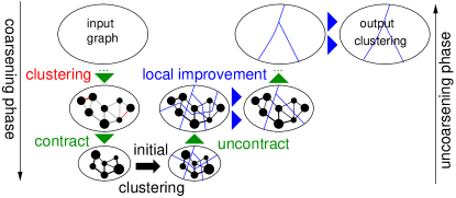
Figure 1: Multilevel scheme.

Multilevel Scheme.

A successful heuristic for vertex partitioning is the multilevel [15] approach, illustrated in Figure 1. It recursively computes a clustering and contracts it to coarsen the graph into smaller graphs that maintain the same basic structure as the input graph. An initial partitioning algorithm is applied to the smallest (coarsest) graph and then the contraction is undone. At each level, a local search method is used to improve the partitioning induced by the coarser level. Contracting a cluster of vertices $C=\left\{u_{1},\ldots,u_{\ell}\right\}$ involves replacing them with a new vertex $v$ whose weight is the sum of the weights of the clustered vertices and is connected to all elements $w\in\bigcup_{i=1}^{\ell}N(u_{i})$, $\omega(\left\{v,w\right\})=\sum_{i=1}^{\ell}\omega(\left\{u_{i},w\right\})$. This ensures that the transfer of partitions from a coarser to a finer level maintains the edge-cut. The uncontraction of a vertex undoes the contraction. Local search moves vertices between blocks to reduce the objective.

SPAC Transformation.

The SPAC transformation [33] provides a means to employ a vertex partitioning tool on a transformed graph $G^{\prime}$, which is derived from the original graph $G$, and subsequently apply the derived vertex partition to establish an edge partition for $G$. The transformation assumes an undirected, unweighted graph $G=(V,E)$ as input. The SPAC graph $G^{\prime}=(V^{\prime},E^{\prime})$ is then constructed in two phases: In the split phase, each vertex $v\in V$ generates $d(v)$ split vertices $S_{v}\coloneqq\{v^{\prime}_{1},...,v^{\prime}_{d(v)}\}\subseteq V^{\prime}$. The connect phase introduces two kinds of edges in $E^{\prime}$, dominant edges and auxiliary edges. First, it assigns a dominant edge $e^{\prime}=(\mu^{\prime}_{i},v^{\prime}_{j})$ in $G^{\prime}$ for each edge $e=(u,v)$ in $G$. Dominant edges are created with infinite weight $\omega(e^{\prime})=\infty$. Second, it introduces as many auxiliary edges $e^{\prime\prime}$ as necessary to create a path connecting the vertices in the set $S_{v}$ for each vertex $v\in V$. Auxiliary edges are created with unitary weight $\omega(e^{\prime\prime})=1$. A visual representation of the SPAC transformation is provided in Figure 3. Due to the infinite weight of dominant edges, vertex partitioning tools usually refrain from splitting them, causing both endpoints of a dominant edge to be grouped in the same block (alternatively, straightforward heuristics can compel both endpoints of dominant edges to belong to the same block). Next, the block assigned to both endpoints of each dominant edge is assigned to the edge in $G$ that induced the corresponding dominant edge, thereby resulting in an edge partition of $G$. The SPAC method is particularly effective in practical scenarios and yields a sound, provable approximation factor under specific balance constraints. Specifically, it approximates the balanced edge partitioning problem within $\mathcal{O}(\Delta\sqrt{\log{n}\log{k}})$, where $\Delta$ is the maximum degree of $G$ [33].

Buffered Streaming.

In the buffered streaming model, which is an extended version of the one-pass model, we load a $\delta$-sized buffer or batch of input vertices along with their edges. We make block assignment decisions only after the entire batch has been loaded. In practice, the parameter $\delta$ can be chosen in accordance with memory available on the machine. In our contribution, we use a fixed $\delta$ throughout the algorithm. For a predefined batch size of $\delta$, we load and repeatedly partition $\left\lceil{n/\delta}\right\rceil$ batches.

2.2 Related Work

We refer the reader to recent surveys on (hyper)graph partitioning for relevant literature [12, 15, 47]. Here, we focus on the research on streaming vertex and edge partitioning. Most high-quality vertex partitioners for real-world graphs use a multilevel scheme, including KaHIP [44], METIS [28], Scotch [40], and (mt)-KaHyPar [23, 45]. Edge partitioning has been solved directly with multilevel hypergraph partitioners, including PaToH [14], hMETIS [29], KaHyPar [46], Mondriaan [52], MLPart [2], Zoltan [30], SHP [27], UMPa [13], and kPaToH [14].

Streaming (Hyper)Graph Vertex Partitioning.

Tsourakakis et al. [51] introduce Fennel, a one-pass partitioning heuristic adapted from the clustering objective modularity [10]. Fennel minimizes edge-cuts by placing vertices in partitions with more neighboring vertices. Fennel assigns a vertex $v$ to the block $V_{i}$ that maximizes the Fennel gain function $|V_{i}\cap N(v)|-f(|V_{i}|)$, where $f(|V_{i}|)$ is a penalty function to respect a balancing threshold. The authors define the Fennel objective with $f(|V_{i}|)=\alpha\gamma\cdot|V_{i}|^{\gamma-1}$, in which $\gamma$ is a free parameter and $\alpha=m\frac{k^{\gamma-1}}{n^{\gamma}}$. After parameter tuning, the authors define $\gamma=\frac{3}{2}$ and $\alpha=\sqrt{k}\frac{m}{n^{3/2}}$. The time complexity of the algorithm depends on $k$ and is given by $\mathcal{O}(nk+m)$. Stanton and Kliot [48] propose LDG, a greedy heuristic for streaming vertex partitioning. ReLDG and ReFennel are re-streaming versions of LDG and Fennel [39]. Prioritized re-streaming optimizes the ordering of the streaming process [3]. Faraj and Schulz [18] propose HeiStream, which uses a generalized weighted version of the Fennel gain function in a buffered streaming approach. Eyubov et al. [17] introduce FREIGHT, a streaming hypergraph partitioner that adapts the Fennel objective function to partition vertices of a hypergraph on the fly.

Streaming Edge Partitioning.

One-pass streaming edge partitioners include hashing-based partitioners like DBH [53], constrained partitioners like Grid and PDS [26], and HDRF, proposed by Petroni et al. [41]. HDRF exploits the skewed degree distribution of real-world graphs by prioritizing vertex replicas of high-degree vertices. HDRF outperforms DBH, Grid and PDS in solution quality, but has a longer runtime. Zhang et al. [54] introduced SNE, a streaming version of the in-memory edge partitioner NE that utilizes sampling methods. SNE produces better solution quality than HDRF, but with increased memory consumption and runtime [37]. In contrast to one-pass streaming models, RBSEP uses a buffered approach to postpone assignment decisions for edges with limited neighborhood partitioning information available during streaming [49]. Additionally, Mayer et al. [35] introduce ADWISE, a window-based streaming edge partitioner, which uses a dynamic window size that adapts to runtime constraints.

Mayer et al. [36] subsequently propose 2PS-HDRF, a two-phase re-streaming algorithm for edge partitioning, using HDRF as the scoring function in its final partitioning step. The first phase uses a streaming clustering algorithm to gather information about the global graph structure; in the second phase, the graph is re-streamed and partitioned, using information obtained from clustering to make edge partitioning decisions. Mayer et al. [37] modify 2PS-HDRF to propose 2PS-L, which runs in time independent of $k$. 2PS-L switches from HDRF to a new scoring function in the final partitioning step to remove its dependency on $k$, and thus achieves a time complexity of $\mathcal{O}(|E|)$. 2PS-L outperforms ADWISE; it is faster than HDRF and 2PS-HDRF, particularly at large $k$ values, but has lower solution quality. 2PS-HDRF achieves 50% better solution quality than 2PS-L [37].

Sajjad et al. [43] propose HoVerCut, a platform for streaming edge partitioners, which can scale in multi-threaded and distributed systems by decoupling the state from the partitioner. Hoang et al. [24] propose CuSP, a distributed and parallel streaming framework to partition edges based on user-defined policies. CuSP is programmable and can express common streaming edge partitioning strategies from the literature.

3 Buffered Streaming Edge Partitioning

In this section, we present our algorithms, HeiStreamE and FreightE. First, we provide an overview of HeiStreamE’s iterative structure. Subsequently, we detail its input format and buffered graph model, and describe how it uses multilevel vertex partitioning to solve this model. Lastly, we discuss how FreightE builds a hypergraph representation to partition edges using a streaming hypergraph partitioner.

lineno 1 Overall Structure of HeiStreamE

1:for $b\in\{1,\ldots,\lceil\frac{n}{\delta}\rceil\}$ do

2:     Load subgraph $G_{b}$ from input graph $G$

3:     Build model $\beta_{b}$ from $G_{b}$

4:     Run multilevel vertex partitioning on $\beta_{b}$

5:     Permanently assign corresponding edges of $G$ in $G_{b}$ to blocks

3.1 Overall Algorithm

Our framework draws inspiration from HeiStream [18]. We slide through the input graph $G$ by iteratively performing the following series of operations until all the edges of $G$ are assigned to blocks. First, we load a batch composed of $\delta$ vertices and their associated neighborhood, thereby obtaining a subgraph $G_{b}$ contained within the graph $G$. This operation yields edges connecting vertices within the current batch, and edges connecting vertices in the current batch to vertices streamed in previous batches. Second, we build a model $\beta_{b}$ corresponding to $G_{b}$, where the edges of $G_{b}$ are transformed into vertices. Additionally, we incorporate a representation of block assignments from previous batches into $\beta_{b}$. Third, we partition $\beta_{b}$ using a multilevel vertex partitioning algorithm that has been shown to be effective in the context of buffered streaming [18]. We conclude by permanently assigning the edges in $G$ that correspond to vertices in our model $\beta_{b}$ to their respective blocks. Algorithm 1 summarizes the general structure of HeiStreamE, which is illustrated in Figure 2.

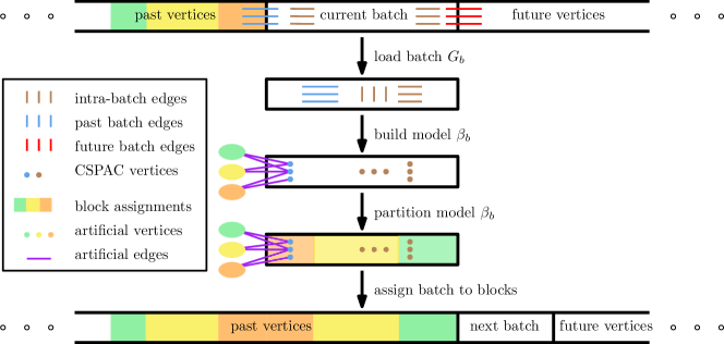
Figure 2: Detailed structure of HeiStreamE. The algorithm starts by loading a batch graph $G_{b}$ consisting of vertices and their edges to the current batch and previous batches. Subsequently, it builds a meaningful model $\beta_{b}$ from the batch graph, transforming edges into vertices, and incorporating a synthetic representation of the assignments made in previous batches. This model is then partitioned using a multilevel algorithm. Lastly, the edges from the loaded batch, which correspond to vertices in the partitioned batch model, are permanently assigned to blocks. This process is repeated for subsequent batches until the entire graph has been partitioned.

3.2 Input and Batch Format

HeiStreamE uses a vertex-centric input format and a buffered streaming approach, which refers to the sequential process of loading and handling the input graph in batches. Within each batch, it loads $\delta$ vertices one at a time along with their neighborhood, where $\delta$ is a parameter that defines the buffer size. Similar input formats are commonly used in streaming algorithms for vertex partitioning [3, 17, 18, 19, 25, 51] and are consistent with graph formats commonly found in publicly available real-world graph datasets, such as the METIS format. Each batch $b\in\{1,\ldots,\lceil\frac{n}{\delta}\rceil\}$ corresponds to a subgraph denoted as $G_{b}=(V_{b},E_{b})$ within the graph $G$. This subgraph is constructed as follows. Its vertex set $V_{b}$ includes the $\delta$ vertices from the current batch, labeled within the domain $[0,\delta-1]$, as well as the $p$ vertices from past batches that share at least one edge with vertices in the current batch, labeled within the domain $[\delta,\delta+p-1]$. Similarly, its edge set $E_{b}$ comprises of edges with one endpoint in the current batch and the other endpoint in either the current batch or previous batches, expressed as $E_{b}=\{(u,v)\in E\mid\text{Batch}(u)=b\land\text{Batch}(v)\leq b\}$. Edges with an endpoint in future batches are discarded, ensuring that each edge belongs exclusively to a unique batch graph $G_{b}$ across all batches.

3.3 Model Construction

Our model construction consists of two steps, detailed in this section. First, using the batch graph $G_{b}$, we create a corresponding Contracted SPlit-And-Connect (CSPAC) graph, denoted as $S^{*}_{b}$. In $S^{*}_{b}$, edges from $G_{b}$ are directly represented as vertices, while vertices from $G_{b}$ are indirectly represented as edges. Subsequently, we create a graph model $\beta_{b}$ based on $S^{*}_{b}$, which incorporates a representation of block assignments from prior batches.

CSPAC Transformation.

The CSPAC transformation is a faster and more condensed variant of the SPAC transformation conceived by Li et al. [33], as described in Section 2.1. Below we explain how the SPAC transformation evolves into the CSPAC transformation, and how this transformation is applied to $G_{b}$ to yield the CSPAC graph $S^{*}_{b}$.

The SPAC graph $G^{\prime}$ of a graph $G$ consists of dominant edges, i.e., edges with a weight of infinity that have a one-to-one correspondence with edges of the original graph, and auxiliary edges, which define a path between vertices of the SPAC graph. The CSPAC transformation is derived from the SPAC graph by contracting the dominant edges into vertices. Due to construction, the dominant edges in $G^{\prime}$ do not share any endpoints; they effectively form a matching, ensuring a consistent contraction. Further, each endpoint of the auxiliary edges is incident to a single dominant edge. Thus, the contraction of all dominant edges produces a coarser graph, in which every vertex represents a unique edge in the original graph $G$, and their connections correspond to the auxiliary edges in graph $G^{\prime}$. The CSPAC transformation is illustrated in Figure 3.

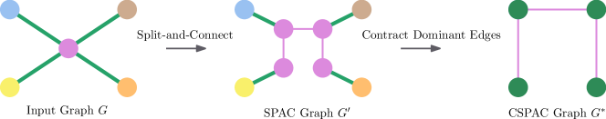
Figure 3: Building SPAC and CSPAC Graphs: The SPAC graph, denoted as $G^{\prime}$, features $d(v)$ split vertices for every vertex $v$ in the original graph $G$. These split vertices are represented in the same color as the vertex they originate from. Every (thick green) edge from $G$ is directly converted into a distinct dominant (thick green) edge in $G^{\prime}$ that connects corresponding split vertices. The auxiliary (thin) edges in $G^{\prime}$, which create a path between split vertices, are depicted in the same color as the split vertices they link. The CSPAC graph $G^{*}$ is formed by contracting the dominant edges of $G^{\prime}$. The vertices in $G^{*}$ represent the edges in $G$, while the edges in $G^{*}$ mirror the auxiliary edges in $G^{\prime}$.

In HeiStreamE, we derive the CSPAC graph $S^{*}_{b}$ directly from the batch graph $G_{b}$, bypassing the construction of the intermediary SPAC graph. The procedure for this direct transformation is as follows. For each vertex $u\in V_{b}$, each of its outgoing edges $e=(u,v)\in E_{b}$ induces a vertex $u^{*}$ in $S^{*}_{b}$, if $u<v$ to avoid redundancy. As each vertex is constructed, it is connected to at most two other vertices in $S^{*}_{b}$ that are induced by other outgoing edges of $u$ in $G_{b}$ to form a path. This way, each undirected edge $e\in E_{b}$, which would have induced a dominant edge in the SPAC graph, is represented as a vertex in $S^{*}_{b}$. Further, each auxiliary edge of the SPAC graph is directly integrated into $S^{*}_{b}$ to form paths between vertices in $S^{*}_{b}$. The direct construction of the CSPAC graph maintains the same computational complexity as the SPAC construction alone, specifically $\mathcal{O}(|V_{b}|+|E_{b}|)$, where $|V_{b}|$ and $|E_{b}|$ are the number of vertices and edges of $G_{b}$ respectively. In practice, building $S^{*}_{b}$ directly from $G_{b}$ offers a time-saving advantage compared to the alternative method of building the SPAC graph and then contracting the dominant edges.

In each batch, $S^{*}_{b}$ has $|E_{b}|$ vertices and $2|E_{b}|-|V_{b}|$ edges, i.e., it is linear in the size of the batch graph $G_{b}$. In contrast to the SPAC graph, the CSPAC graph has fewer vertices and edges. Further, where a vertex partitioner might cut a dominant edge of the SPAC graph, every vertex partition of the CSPAC graph corresponds to a valid edge partition of the original graph. Thus, there is no need for a verification step to transform a vertex partition of $S^{*}_{b}$ into an edge partition of $G_{b}$.

Theorem 3.1 shows that when computing a vertex partition of $S^{*}_{b}$ to minimize the edge-cut, the corresponding edge partition of $G_{b}$ will also have a minimized number of vertex replicas. The SPAC approximation factor shown by Li et al. [33] is also directly valid for $S^{*}_{b}$.

Theorem 3.1.

For any vertex partition $vp(S^{*}_{b})$ of the CSPAC graph $S^{*}_{b}$ with edge-cut $cost(vp(S^{*}_{b}))$, there exists a corresponding edge partition $ep(G_{b})$ of the batch graph $G_{b}$ with a number of vertex replicas $cost(ep(G_{b}))$, satisfying $cost(ep(G_{b}))\leq cost(vp(S^{*}_{b}))$, which establishes a lower bound spanning the set of possible CSPAC graphs $S^{*}_{b}$ associated with $G_{b}$.

Proof 3.2.

Our proof can be delineated through three consecutive claims. (i) The existence of a singular edge partition $ep(G_{b})$ that corresponds to a specified vertex partition $vp(S^{*}_{b})$. (ii) The general validity of the inequality $cost(ep(G_{b}))\leq cost(vp(S^{*}_{b}))$. (iii) The validity of the equality $cost(ep(G_{b}))=cost(vp(S^{*}_{b}))$ for a specific CSPAC graph $S^{*}_{b}$.

Claim (i) trivially holds, as $ep(G_{b})$ stems directly from $vp(S^{*}_{b})$ by virtue of the one-to-one correspondence between edges in $G_{b}$ and vertices in $S^{*}_{b}$. For the proof of assertions (ii) and (iii), consider the following. (a) There can be no replicas of vertices with degree lower than 2. (b) Vertices in $G_{b}$ with a degree lower than 2 are not represented by any edges in $S^{*}_{b}$. (c) Vertices $u$ in $G_{b}$ that possess a degree $d(u)\geq 2$ are represented in $S^{*}_{b}$ through unique, edge-disjoint paths, each connecting the $d(u)$ vertices in $S^{*}_{b}$ corresponding to the edges incident to $u$ in $G_{b}$.

To prove (ii), we show that the number of replicas of any vertex $u$ in $ep(G_{b})$ does not exceed the number of cut edges directly induced by $u$ in $vp(S^{*}_{b})$. From (a) and (b), it trivially holds for vertices with a degree lower than 2. Assuming there are $x>0$ replicas of $u$ in $ep(G_{b})$, it implies that edges incident on $u$ are distributed across $x+1$ nonempty blocks. According to (c), $u$ is uniquely represented by an edge-disjoint path connecting the vertices in $S^{*}_{b}$ that correspond to the edges of $u$ in $G_{b}$. When the vertices of a connected (sub)graph are partitioned into $x+1$ blocks, these blocks themselves are interconnected. Therefore, the edge-cut directly attributable to vertex $u$ is at least $x$, which completes the proof for (ii).

To prove (iii), we show how to build a valid CSPAC graph $S^{*}_{b}$, such that $cost(ep(G_{b}))=cost(vp(S^{*}_{b}))$. For vertices of $G_{b}$ with a degree lower than 2, the equality trivially holds based on (a) and (b). For a vertex $u$ in $ep(G_{b})$ with $x>0$ replicas (edges distributed across $x+1$ nonempty blocks), we create $x+1$ independent paths connecting the vertices in $S^{*}_{b}$ that represent the edges incident to $u$ in $G_{b}$. Vertices in each path are then assigned to a common block. As these paths are between vertices of the same block, they have no cut edges. Subsequently, these paths are interlinked to form a unified path. This introduces exactly $x$ cut edges directly associated with vertex $u$, thereby concluding the proof for condition (iii) and the overall proof.

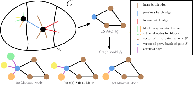
Figure 4: Graph model $\beta_{b}$ construction. $\beta_{b}$ is obtained by appending past assignment decisions to $S^{*}_{b}$. If a vertex of the current batch graph $u\in G_{b}$ has an edge $e=(u,v)$ to a previous batch (colored blue), we connect the CSPAC vertex $u^{*}$ induced by $e$ to artificial vertices representing blocks assigned to edges incident on $v$ as follows: (a) Maximal Mode: $u^{*}$ connects to all blocks incident on $v$ (b) $r$-Subset Mode: $u^{*}$ connects to $r$ random blocks incident on $v$ (c) Minimal Mode: $u^{*}$ connects to the block assigned to the most recently partitioned edge incident on $v$.

Integrating Connectivity Information.

Directly partitioning the CSPAC graph $S^{*}_{b}$ limits the partitioner’s view to the current batch, as $S^{*}_{b}$ does not take into account block assignments from previous batches. Specifically, when assigning a block to a vertex $u^{*}\in S^{*}_{b}$ induced by an edge $e=(u,v)\in E_{b}$, where $u$ is a vertex of the current batch and $v$ is a vertex of some previous batch, the partitioner might replicate $v$ into a new block in the absence of global information. To solve this, we extend the CSPAC graph $S^{*}_{b}$ with connectivity information derived from previous batch assignments to obtain the graph model $\beta_{b}$. We construct $\beta_{b}$ by augmenting $S^{*}_{b}$ with $k$ artificial vertices representing the $k$ partition blocks.

Each artificial vertex $i$ corresponds to an existing partition block $E_{i}$ in its current state, i.e., the weight of each artificial vertex $i$ is the weight of its corresponding block $E_{i}$ filled with edges that have been assigned to it from previous batches. An edge $e=(u,v)\in E_{b}$ of the current batch is represented in our model $\beta_{b}$ as a vertex that connects to an artificial vertex $i$ if $v$ is a vertex of a previous batch whose some incident edge has already been assigned to block $E_{i}$. However, in a streaming setting, there is limited knowledge of edge connectivity, i.e., it is not possible to directly determine which edges from previous batches are adjacent to edges from the current batch. To overcome this constraint, we maintain an array $B$ of size $n$ throughout the streaming process. This array records, for each vertex $u\in V$, block(s) assigned to edges incident on it. Then, in $\beta_{b}$, a vertex $u^{*}\in S^{*}_{b}$ induced by an edge $e=(u,v)\in E_{b}$ is connected to any artificial vertices $i$ representing blocks recorded in $B[v]$. An added benefit of this model construction is that we do not need to maintain a data structure of size $m$ in our algorithm.

We propose three configurations for $\beta_{b}$, which vary in how they use $B$, that we name, in decreasing level of exactness, maximal, $r$-Subset, and minimal. Each configuration has a runtime, memory and solution-quality trade-off. Let $u^{*}$ be a vertex in $S^{*}_{b}$ induced by an edge $e=(u,v)\in E_{b}$. In the maximal model $\beta_{b}$, $u^{*}$ is connected to all artificial vertices $i$ representing blocks recorded in $B[v]$. The memory required to store the array $B$ in the maximal setup is $\mathcal{O}(nk)$. Theorem 3.3 demonstrates that computing a vertex partition of the maximal model $\beta_{b}$ to minimize edge-cut corresponds to an edge partition of $G_{b}$ that contributes a minimized number of new vertex replicas to the overall edge partition of the input graph $G$. In the $r$-Subset model, $u^{*}$ is connected to a sample of r artificial vertices $i$ representing blocks recorded in $B[v]$, where $r$ is a parameter. Here, $B$ is identical as in the maximal setup, but the model $\beta_{b}$ is more concise, allowing for a faster partitioning phase. In the minimal model, $u^{*}$ is connected to a single artificial vertex $i$ representing the most recent block assigned to $v$ in a previous batch. We only store the latest assignment per vertex in $B$, thus the memory requirement is $\mathcal{O}(n)$, and the model $\beta_{b}$ is also more concise than in the other two setups. We illustrate the various configurations in Figure 4.

Theorem 3.3.

For any vertex partition $vp(\beta_{b})$ of the maximal model $\beta_{b}$ with edge-cut $cost(vp(\beta_{b}))$, there exists a corresponding edge partition $ep(G_{b})$ of the batch graph $G_{b}$ that, when incorporated into the already partitioned section of the input graph $G$, introduces a number $\gamma$ of new vertex replicas, satisfying $\gamma\leq cost(vp(\beta_{b}))$.

Proof 3.4.

The only disparity between the CSPAC graph $S^{*}_{b}$ and the maximal model $\beta_{b}$ is the presence of artificial vertices and edges in $\beta_{b}$. If there are no artificial edges in $\beta_{b}$, it implies that none of the edges in the batch graph $G_{b}$ are adjacent to edges in $G$ that have previously been assigned to blocks. In this scenario, Theorem 3.1 provides sufficient grounds to establish the claim. If $\beta_{b}$ contains artificial edges, each artificial edge signifies a unique adjacency in $G$ of an edge in the batch graph $G_{b}$ to edges already assigned to blocks in previous batches. In this scenario, we complete the proof of the claim by noting that the number of cut artificial edges in $vp(\beta_{b})$ cannot be less than the number of new replicas introduced exclusively for vertices contained in previous batches.

3.4 Partitioning

In this section, we describe how we partition our model $\beta_{b}$. We employ a vertex partitioning algorithm on $\beta_{b}$, specifically an adapted version of the multilevel weighted Fennel algorithm utilized in HeiStream [18]. We describe this algorithm and then present a modification to the initial partitioning phase to enhance our runtime performance. Lastly, we discuss possible adaptations to the Fennel parameter $\alpha$.

Multilevel Fennel.

Each per-batch graph model $\beta_{b}$ is partitioned using a multilevel partitioning scheme consisting of three successive phases, coarsening, initial partitioning, and uncoarsening, as depicted in Figure 1.

In the coarsening phase, the algorithm computes a clustering and contracts the graph at each level until it is smaller than a specified threshold. These clusters are computed with label propagation while adhering to size constraints [38]. The clustering algorithm ignores artificial vertices and edges during the coarsening phase, to ensure that they are never contracted and that previous block assignment decisions are available at the coarsest level. For a graph with $n$ vertices and $m$ edges, a single round of size-constrained label propagation can be executed in $\mathcal{O}(n+m)$ time. Initially, each vertex is placed in its own cluster, and in subsequent rounds vertices move to the cluster with the strongest connection, with a maximum of $L$ rounds, where $L$ is a tuning parameter. The coarsening phase ends as soon as the graph has fewer vertices than a threshold of $\mathcal{O}(\max({|\beta_{b}|/k,k}))$, where $|\beta_{b}|$ is the number of vertices of $\beta_{b}$. For large buffer sizes this threshold simplifies to $\mathcal{O}(|\beta_{b}|/k)$, while for small buffer sizes, it becomes $\mathcal{O}(k)$.

Following the coarsening phase, an initial partitioning assigns all non-artificial vertices to blocks using the generalized Fennel algorithm [18] with a strict balancing constraint $L_{\max}$. After initial partitioning, the current solution is transferred to the next finer level by mapping the block assignment of each coarse vertex to its constituent vertices at the finer level. Subsequently, a local search algorithm is applied at each level, which utilizes the size-constrained label propagation approach employed in the contraction phase but with a modified objective function. Specifically, when visiting a non-artificial vertex, we reassign it to a neighboring block to maximize the generalized Fennel gain function while strictly adhering to the balancing constraint $L_{\max}$, considering only adjacent blocks in contrast to the initial partitioning which considers all blocks. This ensures that a single algorithm round remains linear in the current level’s size. Artificial vertices remain stationary during the process, but unlike during coarsening, they are not excluded from label propagation, as they contribute to the generalized Fennel gain function.

Faster Initial Partitioning.

We adopt a modified Fennel function to enhance the initial partitioning step in HeiStreamE and demonstrate that this approach produces a better runtime without a decrease in solution quality.

For small buffer sizes, HeiStream has a linear dependency on $k$ for overall partitioning time, as during initial partitioning each vertex $u\in\beta_{b}$ is assigned to the block with the highest score among all $k$ blocks. To address this dependency, we adopt Eyubov et al.’s strategy [17] from streaming hypergraph partitioning to evaluate scores more efficiently, removing the runtime dependency on $k$. For the current vertex $u\in\beta_{b}$, we categorize $k$ blocks $V_{i}$ into two sets, $S_{1}$ and $S_{2}$, where $V_{i}\in S_{1}$ if a neighbor of $u$ was assigned to it, and $V_{i}\in S_{2}$ otherwise. This allows us to determine the blocks $V_{max}$ and $V_{max}^{\prime}$ that respectively maximize Equation (1) and Equation (2). Then, the block that maximizes the generalized Fennel function is $\max(V_{max},V_{max}^{\prime})$ where

$$V_{max}=\operatorname*{argmax}_{i\in S_{1}}\left\{\sum_{v\in V_{i}\cap N(u)}\omega(u,v)-c(u)f(c(V_{i}))\right\}$$ (1)

$$V_{max}^{\prime}=\operatorname*{argmax}_{i\in S_{2}}\left\{-c(u)f(c(V_{i}))\right\}.$$ (2)

As $c(u)$ remains constant, determining the block $V_{i}\in S_{2}$ that maximizes Equation (2) is equivalent to finding the block $V_{i}$ minimizing $f(c(V_{i}))=\alpha*\gamma*c(V_{i})^{\gamma-1}$, specifically, the $V_{i}\in S_{2}$ with the lowest block weight $c(V_{i})$. In our scheme, $c(V_{i})=c(E_{i})$, that is, the number of edges assigned to block $E_{i}$ of the overall edge partition. This optimized process, facilitated by a priority queue, reduces the evaluation of blocks for each vertex to those assigned to its neighbors and the minimum weight block overall. It results in an optimal block $V_{i}$ for maximizing the generalized Fennel gain function in $\mathcal{O}(d(u)+\log(k))$ time using a binary heap priority queue or $\mathcal{O}(d(u))$ with a bucket priority queue, as suggested in [17], ultimately yielding an overall linear time complexity. With this enhanced approach, the runtime becomes independent of the parameter $k$.

The Parameter $\boldsymbol{\alpha}$.

The authors of Fennel [51], define the parameter $\alpha=\sqrt{k}\frac{m}{n^{3/2}}$ for vertex partitioning of an input graph $G=(V,E)$ with $n$ vertices and $m$ edges. However this choice of $\alpha$ is not directly applicable for edge partitioning in our CSPAC-based model. If we built a single model $\beta_{b}$ for the whole graph $G$ at once, it would have $n^{*}=m$ vertices and a number $m^{*}$ of edges equal to the number of auxiliary edges in $\beta_{b}$. While we know $n^{*}$ immediately, we cannot directly obtain $m^{*}$ without visiting all vertices of the whole graph. Thus, we need to estimate $m^{*}$.

We thus have three distinct approaches for determining the Fennel parameter $\alpha$. In the static $\alpha$ method, we keep $\alpha$ constant across all batches, setting it to $\alpha=\sqrt{k}\frac{m_{approx}}{n^{3/2}}$, where $n^{*}=m/2$, $m_{approx}=y*n^{*}$, and $y$ is a tuning parameter. For the batch $\alpha$ approach, we update $\alpha$ for each batch, calculating it as $\alpha=\sqrt{k}\frac{m_{s}}{n_{s}^{3/2}}$, where $n_{s}$ and $m_{s}$ are the number of vertices and edges of each CSPAC graph $S^{*}_{b}$ respectively. The dynamic $\alpha$ method also updates $\alpha$ per batch. It begins with the static $\alpha$ setting and refines $m_{approx}$ in each batch by computing the number of auxiliary edges, determined through counting vertices of degree less than or equal to 2.

3.5 FreightE

In addition to HeiStreamE, we present FreightE, a fast streaming edge partitioner that uses streaming hypergraph partitioning to assign blocks to edges on the fly. In general, a hypergraph vertex partitioner can partition edges of an input graph $G$ by first transforming it into its dual hypergraph representation $H$, where each edge of $G$ is a hypervertex, and each vertex of $G$ induces a hyperedge spanning its incident edges. Then, a hypergraph vertex partitioner that assigns the hypervertices of $H$ into $k$ blocks, while optimizing for the connectivity metric, directly provides an edge partition of $G$. The intuition behind this approach is that a hypergraph vertex partitioner that optimizes for the connectivity metric directly optimizes the replication factor of the underlying edge partition [15]. In FreightE, we perform the transformation of $G$ into $H$ on the fly as follows. At a given step, we read a vertex of the input graph (METIS format) along with its neighborhood. Each undirected edge in the neighborhood is treated as a unique hypervertex of the hypergraph, and permanently assigned to a block using the FREIGHT streaming hypergraph partitioner [17]. This process is repeated until all vertices along with their neighborhoods are visited, at which point each edge of the input graph is assigned to a block. Following the FREIGHT partitioner, the overall runtime of FreightE is $\mathcal{O}(n+m)$, and memory complexity is $\mathcal{O}(m+k)$. In comparison to HeiStreamE, FreightE is faster, as it does not require the construction of an equivalent CSPAC graph, and requires less memory unless $m\gg n$.

4 Experimental Evaluation

Setup.

We implemented HeiStreamE and FreightE inside the KaHIP framework (using C++) and compiled it using gcc 9.3 with full optimization enabled (-O3 flag). Except for the largest graph instance gsh-2015, all experiments were performed on a single core of a machine consisting of a sixteen-core Intel Xeon Silver 4216 processor running at $2.1$ GHz, $100$ GB of main memory, $16$ MB of L2-Cache, and $22$ MB of L3-Cache running Ubuntu 20.04.1. To facilitate algorithms that required greater memory, gsh-2015 was run on a single core of an alternate machine, consisting of a 64-core AMD EPYC 7702P Processor containing 1 TB of main memory.

Baselines.

We compare HeiStreamE and FreightE against the state-of-the-art streaming algorithm HDRF, as well as the re-streaming algorithms 2PS-HDRF [36] and 2PS-L [37], which require three passes over the input graph. We exclude the following algorithms: SNE [54], as it fails to execute for $k>127$ and is outperformed by 2PS-HDRF [36]; DBH [53], as it ignores past partition assignments and thus has poor solution quality; ADWISE and RBSEP as they have limited global information during streaming, and 2PS-L outperforms them [37].

For comparison with competitors, we obtained implementations of 2PS-HDRF and 2PS-L from their official repository, which also provides an implementation of HDRF. We configure all competitor algorithms with the optimal settings provided by the authors. 2PS-HDRF, 2PS-L and HDRF require a vertex-to-partition table of size $\mathcal{O}(n*k)$, which stores the blocks that each vertex was replicated on. To optimize memory usage, these partitioners can be built with the number of partitions at compile time to only allocate the required amount of memory. Thus, we re-compile them with the CMake flag for the number of blocks for each $k$ value in our experiments. We set the HDRF scoring function parameter $\lambda=1.1$, similar to the authors of 2PS [36]. The provided codes for 2PS-HDRF, 2PS-L, and HDRF in their official repositories set a hard-coded soft limit on the number of partitions to $256$, which we override to test the algorithms with larger $k$ values.

All competitors read a binary edge list format with 32-bit vertex IDs. This allows for faster IO during program execution. Additionally, all competitor programs offer a converter which can load a graph in the standard edge list format, convert it into the binary edge list format, and write it to memory before proceeding. For a fair comparison with HeiStreamE and FreightE, which are capable of reading both text-based (METIS) and binary (adjacency) graphs, we perform experiments with binary graph formats only. Further, we exclude the IO time since the objective of the experiments is to measure the performance of the partitioners and not IO efficiency. Similarly, we exclude the time it takes to convert the graphs into the binary format for all partitioners.

Instances.

Our graph instances for experiments are shown in Appendix Table 2 and are sourced from Ref. [4, 6, 7, 8, 20, 31, 42]. All instances evaluated have been used for benchmarking in previous works on graph partitioning. From these graph instances, we construct three disjoint sets: a tuning set for parameter study experiments, a test set for comparison against state-of-the-art and a set of huge graphs, for which in-memory partitioners ran out of memory on our machine. We set the number of blocks to $k=\{2^{1},2^{2},\dots,2^{14}\}$ for all experiments except those on huge graphs, for which $k$ values are shown in Table 1. We allow an imbalance of $\varepsilon=3\%$ for all partitioners. While streaming, we use the natural order of the vertices in these graphs.

Methodology.

We measure running time, replication factor and memory consumption, i.e., the maximum resident set size for the executed process. When averaging over all instances, we use the geometric mean to give every instance the same influence on the final score. Further, we average all results of each algorithm grouped by $k$, to explore performance with increasing $k$ values. Let the runtime, replication factor or memory consumption be denoted by the score $\sigma_{A}$ for some $k$ partition generated by an algorithm $A$. We express this score relative to others using the following tools: improvement over an algorithm $B$, computed as a percentage $(\frac{\sigma_{A}}{\sigma_{B}}-1)*100\%$ and relative value over an algorithm $B$, computed as $\frac{\sigma_{A}}{\sigma_{B}}$. Additionally, we present performance profiles by Dolan and Moré [16] to benchmark our algorithms. These profiles relate the running time (resp. solution quality, memory) of the slower (resp. worse) algorithms to the fastest (resp. best) one on a per-instance basis, rather than grouped by $k$. Their $x$-axis shows a factor $\tau$ while their $y$-axis shows the percentage of instances for which an algorithm has up to $\tau$ times the running time (resp. solution quality, memory) of the fastest (resp. best) algorithm.

4.1 Parameter Tuning

We tuned the parameters used by HeiStreamE, namely the initial partitioning approach, the selection of the batch graph model $\beta_{b}$ mode and the choice of Fennel $\alpha$, through experiments run on the Tuning Set (see Appendix Table 2). In each experiment we tuned a single parameter with all others constant. We ran all tuning experiments on HeiStreamE, with a buffer size of $\delta=\{32\,768,131\,072,262\,144\}$. In this section, we describe results with $\delta=32\,768$ only, as we found that the choice of the best tuning parameters was independent of buffer size. Our results support the use of $k$-independent initial partitioning, the minimal mode for $\beta_{b}$ and batch $\alpha$ for Fennel’s $\alpha$ parameter for subsequent experiments. Other parameters for the multilevel partitioning scheme, specifically the number of rounds of label propagation during coarsening and uncoarsening, and the size of the coarsest graph, align with optimal values from HeiStream [18].

k-Independent Initial Partitioning.

We evaluated the effect of using our enhanced initial partitioning approach described in Section 3.4. In our implementation, we use a binary heap priority queue to perform increase-key operations in $\mathcal{O}(\log{k})$ time and obtain the block with the smallest weight in $\mathcal{O}(1)$ time. As a baseline, we use the initial partitioning method in HeiStream [18]. Our enhanced initial partitioning approach is, on average, $1.85\times$ faster than the baseline across all $k$ values, and $4.17\times$ faster for $k\geq 256$. The solution quality remains unchanged.

Graph Model Mode.

To choose a suitable per-batch graph model mode among the maximal, r-Subset, and minimal modes, we ran comparisons against a baseline configuration using no mode, i.e., one without any artificial vertices or edges representing block assignment decisions. The minimal model mode produces a solution quality improvement of 11.73% over the baseline of using no mode, which is comparable to the 12.8% increase achieved by the maximal mode. All modes have an increased runtime over the baseline. The minimal mode is $1.11\times$ slower on average than no mode, but is $1.41\times$ and $1.29\times$ faster than the maximal and r-Subset mode respectively. Besides offering a substantial increase in solution quality while being faster than other modes, the minimal mode also has a much lower memory overhead compared to the r-Subset and maximal mode, as we store only one block per vertex $v$ (instead of up to $\min\{k,d(v)\}$ blocks).

Fennel Alpha.

We performed comparisons of the different choices of $\alpha$ among static, batch, and dynamic $\alpha$. We do not observe a significant difference in runtime between the choices for $\alpha$. In terms of replication factor, batch $\alpha$ provides the best solution quality for a majority of $k$ values, particularly for $k>32$. On average, across all instances and all $k$ values, batch $\alpha$ produces $0.86\%$ and $3.27\%$ better solution quality than static and dynamic $\alpha$ respectively. For $k>32$, these averages increase to $2.1\%$ and $5.2\%$ respectively.

4.2 Comparison with State-of-the-Art

We now provide experiments in which we compare HeiStreamE and FreightE against the current state-of-the-art algorithms for (re)streaming edge partitioning, namely, HDRF, 2PS-HDRF and 2PS-L. These experiments were performed on the Test Set and the Huge Set of graphs in Appendix Table 2. Figure 5 gives performance profiles for the Test Set and Table 1 gives detailed per instance results for instances of the Huge Set. We distinguish between buffer sizes by defining, for example, HeiStreamE(32x) as HeiStreamE with a buffer size of $32\,768=32x$ vertices, where $x=1\,024$.

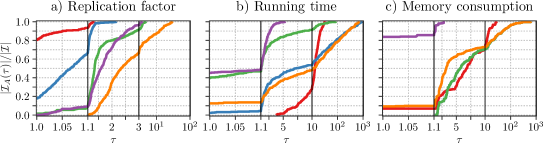
Figure 5: Comparison of HeiStreamE and FreightE with 2PS-HDRF, 2PS-L and HDRF on the Test Set in Appendix Table 2 using performance profiles. Let $\mathcal{A}$ be the set of all algorithms, $\mathcal{I}$ the set of instances, and $q_{A}(I)$ the quality of algorithm $A\in\mathcal{A}$ on instance $I\in\mathcal{I}$. For each algorithm $A$, we plot the fraction of instances $\frac{|\mathcal{I}_{A}(\tau)|}{|\mathcal{I}|}$ (y-axis) where $\mathcal{I}_{A}(\tau):=\left\{I\in\mathcal{I}|q_{A}\leq\tau\cdot min_{A^{\prime}\in\mathcal{A}}q_{A^{\prime}}(I)\right\}$ and $\tau$ is on the x-axis. Includes all $k$ values. Note the logarithmic scale in the final third of the plots. Memory consumption is measured as the maximum resident set size of the program execution.

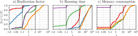
Figure 6: Comparison of HeiStreamE and FreightE with 2PS-HDRF, 2PS-L and HDRF on the Test Set in Appendix Table 2 using performance profiles (see Figure 5 caption for detailed description). Only includes runs with $k\geq 512$. Note the logarithmic scale in the final third of the plots. Memory consumption is measured as the maximum resident set size of the program execution.

Replication Factor.

HeiStreamE(32x) produces better solution quality than state-of-the-art (re)streaming edge partitioners for all $k$ values. The results from our Test Set demonstrate that HeiStreamE(32x) achieves an average improvement in solution quality of 7.56% (or 13.69% when using HeiStreamE(256x)) compared to 2PS-HDRF, which produces the next best solution quality. As displayed in Figure 5a, HeiStreamE(32x) produces better solution quality than 2PS-HDRF in approximately 80% of all Test Set instances. The largest improvement in replication factor that we observed for HeiStreamE(32x) over 2PS-HDRF is of $\approx 53\%$ on graph circuit5M for $k\geq 8192$. Further, HeiStreamE(32x) achieves an average improvement in solution quality of 51.84% percent over 2PS-L, and an average improvement of 202.86% over HDRF, the only other on the fly streaming algorithm presented here. These results from the Test Set are reflected in our experiments on huge graphs, shown in Table 1: HeiStreamE(32x) and HeiStreamE(256x) produce the best solution quality in most instances, providing the best solution quality for all $k$ values for five of the six huge graphs. While FreightE produces lower solution quality than 2PS-L and 2PS-HDRF on most Test Set instances, for $k\geq 512$, FreightE, produces 9.88% higher solution quality than 2PS-L on average. FreightE produces 87.28% better solution quality than HDRF on average across all Test Set instances and $k$ values. The same trends for FreightE are reflected in our results on huge graphs.

Runtime.

HeiStreamE(32x) is on average slower than 2PS-HDRF and HDRF for $k\leq 256$; however, since its runtime is not linearly dependent on $k$, HeiStreamE is substantially faster than 2PS-HDRF and HDRF for higher $k$ values (Figure 6b). On the Test Set, HeiStreamE(32x) is on average $6.7\times$ faster than 2PS-HDRF and $8.7\times$ faster than HDRF for $k\geq 512$. Compared to 2PS-L, whose time complexity is also independent of $k$, HeiStreamE(32x) is on average slower across all instances. Similarly, in our experiments on huge graphs, HeiStreamE(32x) and HeiStreamE(256x) are faster than 2PS-HDRF and HDRF for high $k$ values, but slower than 2PS-L. On the Test Set, FreightE is the fastest algorithm among competitors; it is $1.3\times$ faster than 2PS-L which is the next fastest algorithm. Additionally, it is $9.9\times$ faster than HDRF and $8\times$ faster than 2PS-HDRF on average across all Test Set instances. In our experiments on huge graphs, FreightE is faster than HDRF and 2PS-HDRF on average across all instances, and the fastest algorithm for $k\geq 2\,048$.

Memory Consumption.

Since HeiStreamE(32x) uses a buffered streaming approach, it consumes on average more memory than 2PS-HDRF, 2PS-L and HDRF for $k\leq 256$ on the Test Set; however, since its memory consumption is not asymptotically dependent on $m$ or $k$, HeiStreamE(32x) consumes significantly less memory than 2PS-HDRF, 2PS-L, and HDRF for higher $k$ values. On average, for $k\geq 512$, 2PS-HDRF and 2PS-L use $3.0\times$ more memory than HeiStreamE(32x), and HDRF uses $2.7\times$ more memory than HeiStreamE(32x). Notably, while HeiStreamE(32x) consumes $1.46\times$ more memory on average than 2PS-HDRF and 2PS-L for $k\leq 256$ on the Test Set, in three out of six of the huge graphs, it is more memory efficient than them across all $k$ values. On the Test Set, FreightE consumes significantly less memory than all competitors as shown in Figure 5c. It consumes $4.9\times$ less memory than HDRF and $7.2\times$ less memory than 2PS-L and 2PS-HDRF on average across all instances and all $k$ values. Further, on average, FreightE consumes $16\times$ less memory than 2PS-L and 2PS-HDRF for $k\geq 512$ (Figure 6c). Since FreightE’s memory consumption is linearly dependent on $m$, it is less memory efficient on the huge graphs, which, like other real-world graphs, tend to have many more edges than vertices. FreightE uses more memory than competitors for $k\leq 256$ in five out of six of the huge graphs, but is more memory efficient at high $k$ due to its memory being asymptotically independent of $k$. In our experiments on huge graphs, 2PS-HDRF, 2PS-L and HDRF exceed the available memory on the machine at $k\geq 4\,096$ for uk-2007-05 and webbase-2001, and at $k\geq 8\,192$ for com-friendster. At $k\geq 16\,384$ they exceed the available memory for all graphs, while HeiStreamE and FreightE’s memory consumption is predictable and consistent across $k$.

Table 1: Results of experiments on the Huge Set in Appendix Table 2. Here, we compare HeiStreamE(32x), i.e., HeiStreamE with a buffer size of $32\cdot 1\,024$ (resp. HeiStreamE(256x)), and FreightE with state-of-the-art (re)streaming edge partitioners on huge graph instances, displaying the Replication Factor RF, Running Time RT [s] and Memory Consumption Mem [GB]. The best solution quality for each instance is emboldened. The missing values indicate when an algorithm exceeded the memory of the machine for all graphs except gsh-2015, where the missing value indicates a timeout, i.e., the algorithm exceeded a runtime limit of 24 hours.

$G$	$k$	HeiStreamE(32x)			HeiStreamE(256x)			FreightE			2PS-HDRF			2PS-L			HDRF
		RF	RT	Mem	RF	RT	Mem	RF	RT	Mem	RF	RT	Mem	RF	RT	Mem	RF	RT	Mem
uk-2007-05	4	1.05	3385	15.35	1.05	3648	18.59	1.76	424	12.72	1.12	139	5.92	1.40	142	5.92	2.74	133	2.35
	32	1.05	3707	15.36	1.04	3610	18.54	3.03	427	12.72	1.16	283	5.92	2.05	149	5.92	8.30	718	2.35
	128	1.07	3411	15.37	1.05	3543	18.54	3.59	419	12.72	1.22	918	6.70	2.64	158	6.70	12.45	2589	3.92
	256	1.09	3642	15.37	1.06	3684	18.54	3.81	398	12.71	1.26	1725	8.27	3.06	170	8.27	14.76	4682	7.06
	512	1.10	3407	16.56	1.06	3718	18.35	4.01	373	12.72	1.30	3525	14.50	3.60	201	14.50	17.08	8714	13.32
	1 024	1.13	3421	16.54	1.08	3685	18.54	4.18	371	12.72	1.38	7505	27.03	4.39	279	27.03	19.55	16753	25.86
	2 048	1.18	3406	15.39	1.11	3551	18.54	4.34	371	12.72	1.51	17720	52.10	5.58	527	52.10	22.10	33302	50.93
	4 096	1.24	3419	16.78	1.16	3538	18.54	4.53	370	12.73	-	-	-	-	-	-	-	-	-
	8 192	1.33	3413	16.94	1.23	3580	18.54	4.72	384	12.73	-	-	-	-	-	-	-	-	-
	16 384	1.50	3464	15.67	1.32	3577	18.54	4.97	509	12.73	-	-	-	-	-	-	-	-	-
com-friendster	4	1.62	3356	1.19	1.74	7230	7.08	2.83	357	6.98	1.88	423	3.72	2.08	394	3.72	2.35	251	1.47
	32	4.90	3410	1.22	4.94	7159	7.33	10.71	314	6.98	5.21	865	3.72	6.99	422	3.72	7.97	561	1.47
	128	10.00	3516	1.23	9.53	7370	7.60	18.47	311	6.98	9.00	2159	4.21	12.17	526	4.21	14.53	1523	2.45
	256	13.10	3585	1.26	10.87	7530	7.60	19.79	308	6.98	11.12	3633	5.18	15.05	557	5.18	18.00	2611	4.40
	512	15.92	3681	1.31	11.98	7688	7.59	22.68	306	6.98	13.19	6513	9.05	17.69	615	9.05	21.16	4743	8.31
	1 024	18.05	3742	1.31	12.90	7828	7.76	24.89	312	6.98	15.16	12226	16.87	20.03	702	16.87	23.78	9173	16.14
	2 048	19.00	3916	1.30	13.91	7929	7.73	25.97	339	6.98	16.95	23536	32.51	21.87	858	32.51	25.76	17678	31.78
	4 096	19.77	4024	1.35	15.35	8243	7.84	26.56	358	6.98	18.52	45773	63.80	23.27	1161	63.80	27.15	33753	63.06
	8 192	20.26	4154	1.36	16.90	8325	8.10	26.86	404	6.98	-	-	-	-	-	-	-	-	-
	16 384	21.10	4339	1.33	19.16	8782	8.55	26.90	479	6.98	-	-	-	-	-	-	-	-	-
it-2004	4	1.10	999	11.65	1.10	1019	17.83	1.73	131	4.03	1.15	46	2.54	1.45	47	2.54	2.65	43	0.93
	32	1.09	1000	11.23	1.09	1021	17.70	2.74	116	4.03	1.21	91	2.54	2.12	49	2.54	7.75	229	0.93
	128	1.11	1006	11.22	1.09	1021	18.79	3.20	116	4.03	1.27	271	2.85	2.40	52	2.85	11.70	787	1.54
	256	1.12	1001	11.22	1.09	1027	18.01	3.38	117	4.03	1.31	514	3.47	2.52	55	3.47	13.85	1425	2.77
	512	1.14	1008	11.85	1.10	1007	17.90	3.53	117	4.03	1.35	1033	5.70	2.98	66	5.70	16.15	2684	5.23
	1 024	1.17	1002	11.68	1.12	1013	17.57	3.67	117	4.03	1.39	2132	10.62	3.46	92	10.62	18.51	5237	10.16
	2 048	1.21	1000	11.23	1.16	999	17.86	3.78	116	4.03	1.51	5127	20.46	4.33	157	20.46	20.82	10452	20.00
	4 096	1.27	1013	11.87	1.21	1031	19.47	3.89	118	4.03	1.68	13010	40.15	5.89	356	40.15	22.94	20717	39.69
	8 192	1.38	1020	11.88	1.30	1033	18.08	4.02	116	4.03	1.90	31776	79.53	7.44	817	79.53	24.80	40267	79.07
	16 384	1.53	1032	11.99	1.40	1050	18.09	4.18	151	4.04	-	-	-	-	-	-	-	-	-
sk-2005	4	1.14	2041	12.97	1.16	2126	18.31	2.18	232	7.17	1.17	85	2.94	1.30	88	2.94	2.93	73	1.14
	32	1.25	2036	13.25	1.18	2143	18.32	4.11	236	7.17	1.25	194	2.94	3.06	91	2.94	9.78	391	1.14
	128	1.31	2028	13.02	1.19	2147	19.27	4.90	202	7.17	1.33	630	3.31	4.67	102	3.31	14.13	1459	1.89
	256	1.39	2047	13.10	1.22	2158	19.14	5.16	203	7.17	1.38	1254	4.07	5.65	120	4.07	16.20	2636	3.40
	512	1.46	2052	13.09	1.27	2140	18.35	5.42	203	7.17	1.51	2743	6.98	7.04	159	6.98	18.40	4836	6.42
	1 024	1.55	2035	13.35	1.33	2153	18.35	5.64	203	7.17	1.72	6358	13.02	8.93	261	13.02	20.69	9226	12.45
	2 048	1.63	2064	13.15	1.42	2145	18.43	5.89	205	7.17	1.99	14369	25.09	9.79	452	25.09	23.01	18224	24.53
	4 096	1.75	2076	13.27	1.51	2168	18.37	6.22	207	7.17	2.31	31775	49.24	11.27	997	49.24	25.39	36426	48.67
	8 192	1.86	2095	13.56	1.62	2159	18.38	6.64	211	7.17	2.67	70438	91.45	12.34	2051	91.46	27.95	72800	91.44
	16 384	2.06	2155	13.09	1.78	2185	18.40	7.21	262	7.18	-	-	-	-	-	-	-	-	-
webbase-2001	4	1.06	770	1.33	1.05	782	2.20	1.44	140	3.65	1.10	51	6.32	1.34	50	6.32	2.17	42	2.59
	32	1.08	785	1.31	1.09	790	2.20	1.96	112	3.65	1.16	91	6.32	1.61	53	6.32	4.49	192	2.59
	128	1.09	774	1.31	1.09	789	2.25	2.13	113	3.65	1.20	245	7.18	1.68	57	7.18	5.96	610	4.31
	256	1.09	782	1.38	1.09	799	2.21	2.18	112	3.65	1.22	439	9.04	1.68	61	9.04	6.66	1113	7.75
	512	1.09	790	1.34	1.09	797	2.19	2.21	111	3.65	1.24	817	15.93	1.66	67	15.93	7.33	2117	14.64
	1 024	1.10	751	1.41	1.09	798	2.23	2.24	109	3.65	1.26	1594	29.71	1.66	79	29.71	7.97	4126	28.42
	2 048	1.11	760	1.34	1.10	798	2.20	2.26	108	3.65	1.27	3187	57.26	1.69	108	57.26	8.54	8123	55.97
	4 096	1.13	763	1.46	1.11	798	2.27	2.27	107	3.65	-	-	-	-	-	-	-	-	-
	8 192	1.15	776	1.33	1.12	810	2.16	2.28	107	3.66	-	-	-	-	-	-	-	-	-
	16 384	1.17	797	1.46	1.14	818	2.16	2.30	109	3.66	-	-	-	-	-	-	-	-	-
gsh-2015	4	1.26	22797	45.57	1.25	25128	56.42	1.60	3178	100.49	1.30	2151	52.83	1.70	2149	52.83	3.59	1881	22.10
	32	1.33	22916	45.57	1.32	25522	59.00	2.58	3468	100.35	1.51	4194	52.83	2.74	2195	52.83	16.94	10216	22.10
	128	1.39	23275	46.24	1.39	25421	56.82	3.09	2268	100.49	1.65	11623	60.19	3.52	2393	60.19	26.99	38232	36.83
	256	1.42	23194	45.57	1.41	25403	59.94	3.28	2253	100.49	1.70	21482	77.33	3.87	2545	77.33	31.09	64247	66.29
	512	1.46	23299	45.57	1.43	25495	59.32	3.44	2264	100.49	1.77	41227	136.25	4.21	2751	136.25	-	-	-

5 Conclusion

In this work, we propose HeiStreamE, a buffered streaming edge partitioner that achieves state-of-the-art solution quality, and FreightE, a highly efficient streaming edge partitioner that uses streaming hypergraph partitioning to assign blocks to edges on the fly. HeiStreamE processes the input graph in batches, constructs a novel graph transformation on the per-batch graph model, extends it with global partitioning information, and partitions it with a multilevel scheme. Aside from hashing-based streaming partitioners, which have poor solution quality, HeiStreamE and FreightE are the only known streaming edge partitioners whose runtime and memory consumption are both linear and asymptotically independent of the number of blocks of partition $k$. Our experiments demonstrate that HeiStreamE and FreightE consistently outperform all existing (re)streaming edge partitioners with regard to vertex replication metrics and runtime respectively. Additionally, HeiStreamE uses less memory than high-quality (re)streaming edge partitioners at $k\geq 256$ or when the graph has far more edges than vertices, as is the case for most real-world networks. Our findings underscore HeiStreamE as a highly memory-efficient and effective solution for streaming edge partitioning of large-scale graphs.

Appendix A Instance Properties

Table 2: Graphs used for experiments. The roadNet graphs, wiki graphs, web-Google, web-NotreDame, and all social, co-purchasing, and autonomous systems graphs were obtained from the publicly available SNAP dataset [31]. We also used graphs from the 10th DIMACS Implementation Challenge, namely eu-2005, in-2004 and uk-2007-05 [4]. Any remaining graphs are available on the network repository website [42] or on the Laboratory for Web Algorithmics website [6, 7, 8]. For our experiments, we converted these graphs to a vertex-stream format (METIS) while removing parallel edges, self-loops, and directions, and assigning unitary weight to all vertices and edges. If a graph was unavailable in an equivalent edge list format, we converted the METIS format into the edge list format while preserving edge order for fairness during streaming.

References

- [1] Dan Alistarh, Jennifer Iglesias, and Milan Vojnovic. Streaming min-max hypergraph partitioning. In Advances in Neural Information Processing Systems, pages 1900–1908, 2015. doi:10.5555/2969442.2969452.
- [2] C.J. Alpert, Jen-Hsin Huang, and Andrew Kahng. Multilevel circuit partitioning. Computer-Aided Design of Integrated Circuits and Systems, IEEE Transactions on, 17:655 – 667, 09 1998. doi:10.1109/43.712098.
- [3] Amel Awadelkarim and Johan Ugander. Prioritized restreaming algorithms for balanced graph partitioning. In Proc. of the 26th ACM SIGKDD Intl. Conf. on Knowledge Discovery & Data Mining, pages 1877–1887, 2020. doi:10.1145/3394486.3403239.
- [4] David A. Bader, Henning Meyerhenke, Peter Sanders, Christian Schulz, Andrea Kappes, and Dorothea Wagner. Benchmarking for graph clustering and partitioning. In Encyclopedia of Social Network Analysis and Mining, pages 73–82. 2014. doi:10.1007/978-1-4614-6170-8\_23.
- [5] David A. Bader, Henning Meyerhenke, Peter Sanders, and Dorothea Wagner, editors. Graph Partitioning and Graph Clustering, 10th DIMACS Implementation Challenge Workshop, Georgia Institute of Technology, Atlanta, GA, USA, February 13-14, 2012. Proceedings, volume 588 of Contemporary Mathematics. American Mathematical Society, 2013. URL: http://dblp.uni-trier.de/db/conf/dimacs/dimacs2012.html.
- [6] Paolo Boldi, Andrea Marino, Massimo Santini, and Sebastiano Vigna. BUbiNG: Massive crawling for the masses. In Proceedings of the Companion Publication of the 23rd International Conference on World Wide Web, pages 227–228. International World Wide Web Conferences Steering Committee, 2014.
- [7] Paolo Boldi, Marco Rosa, Massimo Santini, and Sebastiano Vigna. Layered label propagation: A multiresolution coordinate-free ordering for compressing social networks. In Sadagopan Srinivasan, Krithi Ramamritham, Arun Kumar, M. P. Ravindra, Elisa Bertino, and Ravi Kumar, editors, Proceedings of the 20th international conference on World Wide Web, pages 587–596. ACM Press, 2011.
- [8] Paolo Boldi and Sebastiano Vigna. The WebGraph framework I: Compression techniques. In Proc. of the 13th Int. World Wide Web Conf. (WWW 2004), pages 595–601, Manhattan, USA, 2004. ACM Press.
- [9] Florian Bourse, Marc Lelarge, and Milan Vojnovic. Balanced Graph Edge Partition. In Proc. of 20th ACM SIGKDD Intl. Conf. on Knowledge Discovery and Data Mining, KDD ’14, pages 1456–1465. ACM, 2014. doi:10.1145/2623330.2623660.
- [10] Ulrik Brandes, Daniel Delling, Marco Gaertler, Robert Gorke, Martin Hoefer, Zoran Nikoloski, and Dorothea Wagner. On modularity clustering. IEEE transactions on knowledge and data engineering, 20(2):172–188, 2007. doi:10.1109/TKDE.2007.190689.
- [11] Thang Nguyen Bui and Curt Jones. Finding Good Approximate Vertex and Edge Partitions is NP-Hard. Information Processing Letters, 42(3):153–159, 1992. doi:10.1016/0020-0190(92)90140-Q.
- [12] Aydın Buluç, Henning Meyerhenke, Ilya Safro, Peter Sanders, and Christian Schulz. Recent Advances in Graph Partitioning, pages 117–158. Springer Intl. Publishing, Cham, 2016. doi:10.1007/978-3-319-49487-6_4.
- [13] Ü. V. Çatalyürek, M. Deveci, K. Kaya, and B. Uçar. UMPa: A Multi-objective, Multi-level Partitioner for Communication Minimization. In 10th DIMACS Impl. Challenge Workshop: Graph Partitioning and Graph Clustering. Georgia Institute of Technology, Atlanta, GA, February 13-14 2012.
- [14] Ümit V. Çatalyürek and Cevdet Aykanat. Patoh (partitioning tool for hypergraphs). In Encyclopedia of Parallel Computing, pages 1479–1487. Springer, 2011. doi:10.1007/978-0-387-09766-4\_93.
- [15] Ümit V. Çatalyürek, Karen D. Devine, Marcelo Fonseca Faraj, Lars Gottesbüren, Tobias Heuer, Henning Meyerhenke, Peter Sanders, Sebastian Schlag, Christian Schulz, Daniel Seemaier, and Dorothea Wagner. More recent advances in (hyper)graph partitioning. ACM Computing Surveys, 55:1–38, 2023. doi:doi.org/10.1145/3571808.
- [16] Elizabeth D. Dolan and Jorge J. Moré. Benchmarking optimization software with performance profiles. Mathematical Programming, 91(2):201–213, Jan 2002. doi:10.1007/s101070100263.
- [17] Kamal Eyubov, Marcelo Fonseca Faraj, and Christian Schulz. FREIGHT: Fast Streaming Hypergraph Partitioning. In Loukas Georgiadis, editor, Intl. Sym. on Experimental Algorithms (SEA), volume 265 of Leibniz International Proceedings in Informatics (LIPIcs), pages 15:1–15:16, Dagstuhl, Germany, 2023. Schloss Dagstuhl – Leibniz-Zentrum für Informatik. URL: https://drops.dagstuhl.de/opus/volltexte/2023/18365, doi:10.4230/LIPIcs.SEA.2023.15.
- [18] Marcelo Fonseca Faraj and Christian Schulz. Buffered streaming graph partitioning. ACM J. Exp. Algorithmics, 27:1.10:1–1.10:26, 2022. doi:10.1145/3546911.
- [19] Marcelo Fonseca Faraj and Christian Schulz. Recursive multi-section on the fly: Shared-memory streaming algorithms for hierarchical graph partitioning and process mapping. In 2022 IEEE Intl. Conf. on Cluster Computing (CLUSTER), pages 473–483, 2022. URL: https://ieeexplore.ieee.org/document/9912716, doi:10.1109/CLUSTER51413.2022.00057.
- [20] Daniel Funke, Sebastian Lamm, Peter Sanders, Christian Schulz, Darren Strash, and Moritz von Looz. Communication-free massively distributed graph generation. In 2018 IEEE International Parallel and Distributed Processing Symposium (IPDPS), pages 336–347, 2018. doi:10.1109/IPDPS.2018.00043.
- [21] Michael R. Garey, David S. Johnson, and Larry Stockmeyer. Some Simplified NP-Complete Problems. In Proc. of the 6th ACM Sym. on Theory of Computing, (STOC), pages 47–63. ACM, 1974. doi:10.1145/800119.803884.
- [22] Joseph E Gonzalez, Yucheng Low, Haijie Gu, Danny Bickson, and Carlos Guestrin. Powergraph: Distributed graph-parallel computation on natural graphs. In Presented as part of the 10th USENIX Sym. on Operating Systems Design and Implementation (OSDI 12), pages 17–30, 2012. doi:10.5555/2387880.2387883.
- [23] Lars Gottesbüren, Tobias Heuer, Peter Sanders, and Sebastian Schlag. Scalable Shared-Memory Hypergraph Partitioning. In Proc. of the Sym. on Algorithm Engineering and Experiments ALENEX, pages 16–30, 2021. doi:10.1137/1.9781611976472.2.
- [24] Loc Hoang, Roshan Dathathri, Gurbinder Gill, and Keshav Pingali. Cusp: A customizable streaming edge partitioner for distributed graph analytics. In 2019 IEEE Intl. Parallel and Distributed Processing Sym. (IPDPS), pages 439–450. IEEE, 2019. doi:10.1109/IPDPS.2019.00054.
- [25] Nazanin Jafari, Oguz Selvitopi, and Cevdet Aykanat. Fast shared-memory streaming multilevel graph partitioning. Journal of Parallel and Distributed Computing, 147:140–151, 2021. doi:10.1016/j.jpdc.2020.09.004.
- [26] Nilesh Jain, Guangdeng Liao, and Theodore L. Willke. Graphbuilder: Scalable graph etl framework. In First International Workshop on Graph Data Management Experiences and Systems, GRADES ’13, New York, NY, USA, 2013. Association for Computing Machinery. doi:10.1145/2484425.2484429.
- [27] Igor Kabiljo, Brian Karrer, Mayank Pundir, Sergey Pupyrev, Alon Shalita, Yaroslav Akhremtsev, and Alessandro Presta. Social hash partitioner: A scalable distributed hypergraph partitioner. Proc. VLDB Endow., 10(11):1418–1429, 2017. URL: http://www.vldb.org/pvldb/vol10/p1418-pupyrev.pdf, doi:10.14778/3137628.3137650.
- [28] George Karypis and Vipin Kumar. A fast and high quality multilevel scheme for partitioning irregular graphs. SIAM J. Sci. Comput., 20(1):359–392, 1998. doi:10.1137/S1064827595287997.
- [29] George Karypis and Vipin Kumar. Multilevel k-way hypergraph partitioning. In Proceedings of the 36th Conference on Design Automation, pages 343–348. ACM Press, 1999. doi:10.1145/309847.309954.
- [30] R.T. Heaphy R.G. Bisseling K.D. Devine, E.G. Boman and Ümit Çatalyürek. Parallel hypergraph partitioning for scientific computing. International Conference on Parallel and Distributed Processing (IPDPS), 20:124–124, 2006.
- [31] Jure Leskovec. Stanford Network Analysis Package (SNAP), 2013.
- [32] Jure Leskovec, Kevin J. Lang, Anirban Dasgupta, and Michael W. Mahoney. Community structure in large networks: Natural cluster sizes and the absence of large well-defined clusters. CoRR, abs/0810.1355, 2008. URL: http://arxiv.org/abs/0810.1355, arXiv:0810.1355.
- [33] Lingda Li, Robel Geda, Ari B. Hayes, Yan-Hao Chen, Pranav Chaudhari, Eddy Z. Zhang, and Mario Szegedy. A simple yet effective balanced edge partition model for parallel computing. Proc. ACM Meas. Anal. Comput. Syst., 1(1):14:1–14:21, 2017. doi:10.1145/3084451.
- [34] Yucheng Low, Danny Bickson, Joseph Gonzalez, Carlos Guestrin, Aapo Kyrola, and Joseph M. Hellerstein. Distributed graphlab: A framework for machine learning and data mining in the cloud. 5(8):716–727, apr 2012. doi:10.14778/2212351.2212354.
- [35] Christian Mayer, Ruben Mayer, Muhammad Adnan Tariq, Heiko Geppert, Larissa Laich, Lukas Rieger, and Kurt Rothermel. Adwise: Adaptive window-based streaming edge partitioning for high-speed graph processing. In 2018 IEEE 38th Intl. Conf. on Distributed Computing Systems (ICDCS), pages 685–695. IEEE, 2018. doi:10.1109/ICDCS.2018.00072.
- [36] Ruben Mayer, Kamil Orujzade, and Hans-Arno Jacobsen. 2ps: High-quality edge partitioning with two-phase streaming. CoRR, abs/2001.07086, 2020. URL: https://arxiv.org/abs/2001.07086, arXiv:2001.07086.
- [37] Ruben Mayer, Kamil Orujzade, and Hans-Arno Jacobsen. Out-of-core edge partitioning at linear run-time. In 38th IEEE International Conference on Data Engineering, ICDE 2022, Kuala Lumpur, Malaysia, May 9-12, 2022, pages 2629–2642. IEEE, 2022. doi:10.1109/ICDE53745.2022.00242.
- [38] Henning Meyerhenke, Peter Sanders, and Christian Schulz. Partitioning complex networks via size-constrained clustering. In Experimental Algorithms - 13th International Symposium, SEA, volume 8504 of LNCS, pages 351–363. Springer, 2014. doi:10.1007/978-3-319-07959-2\_30.
- [39] Joel Nishimura and Johan Ugander. Restreaming graph partitioning: simple versatile algorithms for advanced balancing. In Proc. of the 19th ACM SIGKDD international conference on Knowledge discovery and data mining, pages 1106–1114, 2013. doi:10.1145/2487575.2487696.
- [40] François Pellegrini and Jean Roman. Experimental analysis of the dual recursive bipartitioning algorithm for static mapping. Technical report, TR 1038-96, LaBRI, URA CNRS 1304, Univ. Bordeaux I, 1996.
- [41] Fabio Petroni, Leonardo Querzoni, Khuzaima Daudjee, Shahin Kamali, and Giorgio Iacoboni. Hdrf: Stream-based partitioning for power-law graphs. In Proc. of the 24th ACM Intl. on Conf. on Information and Knowledge Management, pages 243–252, 2015. doi:10.1145/2806416.2806424.
- [42] Ryan A. Rossi and Nesreen K. Ahmed. The network data repository with interactive graph analytics and visualization. http://networkrepository.com, 2015.
- [43] Hooman Peiro Sajjad, Amir H Payberah, Fatemeh Rahimian, Vladimir Vlassov, and Seif Haridi. Boosting vertex-cut partitioning for streaming graphs. In 2016 IEEE Intl. Congress on Big Data (BigData Congress), pages 1–8. IEEE, 2016. doi:10.1109/BigDataCongress.2016.10.
- [44] Peter Sanders and Christian Schulz. Think Locally, Act Globally: Highly Balanced Graph Partitioning. In 12th Intl. Sym. on Experimental Algorithms (SEA), LNCS. Springer, 2013. doi:10.1007/978-3-642-38527-8_16.
- [45] Sebastian Schlag, Vitali Henne, Tobias Heuer, Henning Meyerhenke, Peter Sanders, and Christian Schulz. k-way hypergraph partitioning via n-level recursive bisection. In Proceedings of the Eighteenth Workshop on Algorithm Engineering and Experiments, ALENEX, pages 53–67. SIAM, 2016. doi:10.1137/1.9781611974317.5.
- [46] Sebastian Schlag, Christian Schulz, Daniel Seemaier, and Darren Strash. Scalable edge partitioning. In Proc. of the 21st Workshop on Algorithm Engineering and Experiments, ALENEX 2019, San Diego, CA, USA, January 7-8, 2019, pages 211–225. SIAM, 2019. doi:10.1137/1.9781611975499.17.
- [47] Christian Schulz and Darren Strash. Graph partitioning: Formulations and applications to big data. In Encyclopedia of Big Data Technologies. Springer, 2019. doi:10.1007/978-3-319-63962-8\_312-2.
- [48] Isabelle Stanton and Gabriel Kliot. Streaming graph partitioning for large distributed graphs. In Proc. of the 18th ACM SIGKDD international conference on Knowledge discovery and data mining, pages 1222–1230, 2012. doi:10.1145/2339530.2339722.
- [49] Monireh Taimouri and Hamid Saadatfar. Rbsep: a reassignment and buffer based streaming edge partitioning approach. Journal of Big Data, 6(1):92, Oct 2019. doi:10.1186/s40537-019-0257-5.
- [50] Fatih Taşyaran, Berkay Demireller, Kamer Kaya, and Bora Uçar. Streaming Hypergraph Partitioning Algorithms on Limited Memory Environments. In HPCS 2020 - Intl. Conf. on High Performance Computing & Simulation, pages 1–8. IEEE, 2021. URL: https://hal.archives-ouvertes.fr/hal-03182122.
- [51] Charalampos Tsourakakis, Christos Gkantsidis, Bozidar Radunovic, and Milan Vojnovic. Fennel: Streaming graph partitioning for massive scale graphs. In Proc. of the 7th ACM international conference on Web search and data mining, pages 333–342, 2014. doi:10.1145/2556195.2556213.
- [52] Brendan Vastenhouw and Rob Bisseling. A two-dimensional data distribution method for parallel sparse matrix-vector multiplication. SIAM Review, 47, 06 2002. doi:10.1137/S0036144502409019.
- [53] Cong Xie, Ling Yan, Wu-Jun Li, and Zhihua Zhang. Distributed power-law graph computing: Theoretical and empirical analysis. In Advances in Neural Information Processing Systems 27: Annual Conf. on Neural Information Processing Systems, pages 1673–1681, 2014. URL: https://proceedings.neurips.cc/paper/2014/hash/67d16d00201083a2b118dd5128dd6f59-Abstract.html.
- [54] Chenzi Zhang, Fan Wei, Qin Liu, Zhihao Gavin Tang, and Zhenguo Li. Graph edge partitioning via neighborhood heuristic. In Proc. of the 23rd ACM SIGKDD Intl. Conf. on Knowledge Discovery and Data Mining, pages 605–614. ACM, 2017. doi:10.1145/3097983.3098033.