Chaotic fields behave universally out of equilibrium

Abstract

Chaotic dynamics is always characterized by swarms of unstable trajectories, unpredictable individually, and thus generally studied statistically. It is often the case that such phase-space densities relax exponentially fast to a limiting distribution, that rules the long-time average of every observable of interest. Before that asymptotic time scale, the statistics of chaos is generally believed to depend on both the initial conditions and the chosen observable. I show that this is not the case for a widely applicable class of models, that feature a phase-space (‘field’) distribution common to all pushed-forward or integrated observables, while the system is still relaxing towards statistical equilibrium or a steady state. This universal profile is determined by both leading and first subleading eigenfunctions of the transport operator (Koopman or Perron-Frobenius) that maps phase-space densities forward or backwards in time.

1 Introduction

As a fact of nature, chaos is unpredictable, due to the extreme sensitivity of trajectories to initial conditions, and the finite precision of our computers. Impossible as it is to solve the problem of motion, practitioners resort to the tools of statistical mechanics to estimate averages and fluctuations of observables of interest (energy, diffusion constant, Lyapunov exponents, vorticity, etc.). That feat is achievable for long-time evolution, provided that the system in exam be ergodic, and that it asymptotically relax to a limiting distribution usually called natural measure, which may be used as a weighting function for phase-space averages.

The natural measure (or invariant density) is the leading eigenfunction of the Perron-Frobenius transport operator ${\cal L}_{t}$ [7], that evolves densities in time throughout the phase space, and whose leading eigenvalue determines the escape rate. As the resolvent to the Liouville equation, this operator is linear, but infinite dimensional [8]. Especially in the Koopman form (adjoint of Perron-Frobenius), transport operators have found countless applications in recent years [25, 20, 10, 1], thanks to the genericity of the Markov property throughout modelling [18], and so have their finite-dimensional discretizations [13, 19, 24, 27], which lend themselves to a faster time-iteration and a practical spectral analysis.

Spectrum wise, the subleading eigenvalue yields information on the speed of relaxation of the system to statistical equilibrium or steady state, and on the typical time scale of the decay of correlations. The corresponding eigenfunction defines the path leading to equilibrium in multistable systems [23], while, in strong chaos [31] and two-dimensional vector fields [6], it was shown to exhibit similar patterns as the distribution of finite-time Lyapunov exponents, that is the field of local instabilities.

The present report demonstrates that the first two eigenfunctions of the transfer operator spectrum not only govern the distribution of the Lyapunov exponents, but any field derived from numerically integrated trajectories (‘Lagrangian’ point of view in fluid dynamics), that is the phase-space distribution of an observable pushed downstream at an intermediate timescale before relaxation to equilibrium or steady state.

2 Time-dependent statistics of chaotic observables

2.1 Mapping phase-space averages

Given an observable $a(x)$ defined as a function or an operator in the phase space ${\cal M}$, its expectation value may be written as

$$\langle a\rangle=\frac{1}{\mu_{\cal M}(\rho)}\int a(x)\rho(x)\,dx\,,$$ (1)

where $\rho(x)$ is the phase space density, that is the frequency with wich trajectories visit ${\cal M}$, while $\mu_{\cal M}(\cdot)$ is the Lebesgue measure over ${\cal M}$. Both $a$ and $\rho$ are functions of the dynamical variable $x$, that is advected by a flow $f^{t}(x)$ as time proceeds. As a result, the expectation value Eq. 1 itself depends on time as

$$\langle a^{t}\rangle=\frac{1}{\mu_{\cal M}(\rho^{t})}\int a(f^{t}(x))\rho(x)\,dx\,.$$ (2)

The ‘downstream’ (or pushed-forward) observable $a(f^{t}(x))$ may also be expressed through the action of the Koopman operator, $\left[{\cal L}^{\dagger}_{t}a\right](x)=a(f^{t}(x))$, which is linear and rewrites the integral in Eq. 2 as

$$\int\left[{\cal L}^{\dagger}_{t}a\right](x)\rho(x)\,dx\,=\int a(x)\left[{\cal L}_{t}\rho\right](x)\,dx$$

$$=\int dx\,a(x)\,\int dx_{0}\,\delta\left(x-f^{t}(x_{0})\right)\rho(x_{0})\,,$$ (3)

meaning that one can shift the action of the push-forward operator ${\cal L}^{\dagger}_{t}$ from the field $a$ to the density $\rho$, that is instead pulled back by the adjoint ${\cal L}_{t}$ of the Koopman operator.

2.2 Chaos and spectral expansions

The Perron-Frobenius operator ${\cal L}_{t}$ is a formal solution to the Liouville equation $\partial_{t}\rho+\nabla\cdot(\rho\,v)=0$, where $\dot{x}=v(x)$ is the dynamical system generating the flow $f^{t}(x)$. In chaotic systems with no escape and with a proper choice of function space [5], the Perron-Frobenius spectrum has an isolated, unitary eigenvalue, whose (‘leading’) eigenfunction is called natural measure or invariant density [16]. The natural measure is the weight to every phase-space average, and, as such, its successful determination enables us to evaluate any long-term averaged observable under the ergodicity assumption. For an open system, the leading eigenvalue is less than unity and its logarithm is the escape rate, whereas the associate eigenfunction is called conditionally invariant density. If the system is chaotic and mixing, that is time-correlations decay exponentially fast, the subleading spectrum of ${\cal L}_{t}$ can be discrete and subunitary, with the second eigenvalue yielding the decay rate of any initial density to the natural measure. It therefore refers to an intermediate timescale, where the system is still in the process of relaxation towards either statistical equilibrium or a steady state.

The meaning and avail of the second eigenfunction is the object of the present study, and it is revealed by expanding the piece $\left[{\cal L}_{t}\rho\right](x)$ in Eq. 3:

$$\int a(x)\left[{\cal L}_{t}\rho\right](x)\,dx\,=\sum_{j}b_{j}\,e^{-\gamma_{j}t}\int a(x)\phi_{j}(x)\,dx$$ (4)

is still the numerator of the downstream average $\langle a^{t}\rangle$, that depends on time and initial conditions, and thus it is not so meaningful before the system has reached statistical equilibrium. For that reason, it is sensible to go beyond the single moments and work out an expression for the full phase-space (‘field’) distribution of $a^{t}$ that involves the spectrum of ${\cal L}_{t}$, which, importantly, does not depend on the observable chosen. Such feat can be achieved by first identifying the initial conditions in Eq. 4 with the coefficients

$$b_{j}=\int\rho(x)\varphi_{j}(x)\,dx\,,$$ (5)

where the $\varphi_{j}(x)$ are eigenfunctions of the Koopman operator ${\cal L}^{\dagger}_{t}$, and then by setting the initial density to $\rho(x)=\delta(x-x_{0})$, that is entirely concentrated in one point.

That done, the expectation value Eq. 2 becomes the distribution

$$a(f^{t}(x_{0}))=\frac{1}{\mu_{\cal M}(\rho^{t})}\sum_{j}\varphi_{j}(x_{0})\,e^{-\gamma_{j}t}\int a(x)\phi_{j}(x)\,dx\,.$$ (6)

The previous expansion will be truncated to the first two terms when considering an intermediate time scale, determined by the spectral gap, as $(\gamma_{1}-\gamma_{0})^{-1}$. On the other hand, the denominator $\mu_{\cal M}(\rho^{t})=\int dx\left[{\cal L}_{t}\rho\right](x)$ is approximated with the first term in the same expansion, so as to obtain, overall,

$$a(f^{t}(x_{0})) \simeq \int a(x)\phi_{0}(x)\,dx+$$ (7)

$$+ \frac{\varphi_{1}(x_{0})}{\varphi_{0}(x_{0})}e^{-(\gamma_{1}-\gamma_{0})t}\int a(x)\phi_{1}(x)\,dx\,,$$

where the first term is the long-time average weighted by the natural measure $\phi_{0}(x)$ (assumed normalized), while the second term characterizes the profile of the distribution by the ratio of the second to the first eigenfunctions of the Koopman operator, that is observable independent. If the system is closed, the escape rate vanishes and thus $\gamma_{0}=0$, while the measure $\mu_{\cal M}(\rho^{t})$ of the density is time independent and may be set to unity. That simplifies the approximate distribution Eq. 7, that now solely depends on the second eigenfunction $\varphi_{1}(x_{0})$ of the Koopman operator for any observable.

If, instead of pushing the observable downstream as $\left[{\cal L}^{\dagger}_{t}a\right](x)=a(f^{t}(x))$, we pull it upstream (or pull back) by means of the adjoint of the Koopman operator, $\left[{\cal L}_{t}a\right](x)$, the above derivation still holds under the same assumptions, but the distribution $\langle a^{-t}\rangle(x_{0})$ now depends on the first two eigenfunctions of the Perron-Frobenius operator ${\cal L}_{t}$ as

$$\frac{a(f^{-t}(x_{0}))}{|J^{t}(f^{-t}(x_{0}))|} \simeq \int a(x)\varphi_{0}(x)\,dx\,+$$ (8)

$$+ \frac{\phi_{1}(x_{0})}{\phi_{0}(x_{0})}e^{-(\gamma_{1}-\gamma_{0})t}\int a(x)\varphi_{1}(x)\,dx\,,$$

assuming $\varphi_{0}(x)$ as normalized. Here $J^{t}(x)$ denotes the Jacobian matrix of the trajectory originating at $x$ and running for time $t$ (definition below), which pops up from the direct application $\left[{\cal L}_{t}\,a\right]$ of the Perron-Frobenius operator to the observable.

2.3 Integrated observables

Of special interest in dynamics are the so-called integrated observables [8], also known as Lagrangian averages [12] (or Birkhoff averages in discrete time)

$$A^{t}(x)=\frac{1}{t}\int_{0}^{t}a\left[f^{\tau}(x)\right]\,d\tau\,,$$ (9)

where the integral is time ordered, that is taken along the trajectory $f^{t}(x)$. Notable examples of integrated observables are the stability (or finite-time Lyapunov) exponent $\ln|\Lambda(x_{0},t)|=\ln\sqrt{||J^{t}(x_{0})||}$, where

$$J^{t}(x_{0})=e^{\int_{0}^{t}d\tau M(f^{\tau}(x_{0}))}\,,\hskip 14.22636ptM_{ij}(x)=\frac{\partial v_{i}(x)}{\partial x_{j}}\,,$$ (10)

and the diffusivity

$$D^{t}(x)=\frac{1}{t}\int_{0}^{t}\left[f^{\tau}(x)-x\right]^{2}\,d\tau\,.$$ (11)

The expectation value Eq. 2 can now be generalized to an integrated observable by replacing $a(f^{t}(x))$ with $A^{t}(x)$, and so the results Eq. 7 and Eq. 8 are also rewritten for $A^{t}$. Yet, the meaning of the field distributions is different: the downstream value $a(f^{t}(x_{0}))$ in Eq. 7 becomes its time-ordered integral $A^{t}(x_{0})$ along the trajectory $f^{t}(x_{0})$, pinned by its initial value $x_{0}$. Conversely, the upstream value $a(f^{-t}(x_{0}))$ is replaced by the time-ordered integral $A^{t}(f^{-t}(x_{0}))$, now a function of the arrival point of the trajectory $f^{-t}(x_{0})\rightarrow x_{0}$. A full account of time-forward and backward Lagrangian averages for chaotic relaxation processes will be given elsewhere [22].

2.4 Noise

The above analysis and predictions may be generalized to chaotic systems subject to weak noise, so that the equations of motion take the Langevin form $\dot{x}=v(x)+\eta(t)$, with the time-uncorrelated and Gaussian-distributed random force $\eta(t)$. The transfer operator ${\cal L}_{t}$ (${\cal L}_{t}^{\dagger}$), that is the formal solution to the associate Fokker-Planck equation [26], features a noisy kernel, for instance [9]

$${\cal L}_{\Delta,t}\,\rho(x)=\frac{1}{\sqrt{4\pi\Delta t}}\int dx\,e^{-(y-f^{t}(x))^{2}/4\Delta t}\rho(x)\,,$$ (12)

for isotropic noise of amplitude $2\Delta$. The operator ${\cal L}_{\Delta,t}$ and its adjoint can be applied to a density $\rho$ as above, or to an observable $a$, to obtain its noisy evolution, whereas the integrated observable Eq. 9 takes the form

$$A^{t}_{\Delta}(x)=\frac{1}{t}\int_{0}^{t}\left[{\cal L}^{\dagger}_{\Delta,\tau}a\right](x)\,d\tau\,.$$ (13)

3 Numerical validation

The above predictions are now tested with two different models of chaos, the perturbed cat map and the Hamiltonian Hénon map. The strategy is that to numerically compute the first two eigenfunctions of the Perron-Frobenius and of the Koopman spectrum, and compare their ratio with the distributions of different pushed-forward, pulled-back, or integrated observables for finite time.

First, the transfer operator is discretized by means of Ulam’s method [29], that is by subdividing the phase space into $N$ intervals ${\cal M}_{i}$ of equal area, and evaluating the transition probabilities from ${\cal M}_{i}$ to ${\cal M}_{j}$:

$$[\mathbf{L}_{t}]_{ij}=\frac{\mu\left({\cal M}_{i}\bigcap f^{t}({\cal M}_{j})\right)}{\mu({\cal M}_{i})}$$ (14)

with $t=1$. The numerator of the transition rate Eq. 14 is estimated with a Monte Carlo method [11], consisting of iterating random initial conditions from each cell ${\cal M}_{i}$ and counting which fraction lands in each ${\cal M}_{j}$.

The finite-dimensional approximation $\mathbf{L}_{t}$ obtained with the Ulam method leverages the Markov property of the systems of our interest, but it is in general unstable and must be used with caution [13]. Still, for certain everywhere unstable (‘hyperbolic’) maps, it was found to well reproduce the leading- and first subleading eigenvalues/eigenfunctions of the Perron-Frobenius operator on a space of characteristic functions supported on the intervals ${\cal M}_{i}$ at sufficiently large $N$ [31].

3.1 Perturbed cat map

It is defined by $f(x)=T_{\epsilon}\circ T[x]$, with $x=(q,p)$,

$$T\left(\begin{array}[]{c}q\\ p\end{array}\right)=\left(\begin{array}[]{cc}1&1\\ 1&2\end{array}\right)\left(\begin{array}[]{c}q\\ p\end{array}\right)\hskip 5.69046pt\mathrm{mod}1\,,$$ (15)

and

$$T_{\epsilon}\left(\begin{array}[]{c}q\\ p\end{array}\right)=\left(\begin{array}[]{c}q-\epsilon\sin 2\pi p\\ p\end{array}\right)\hskip 5.69046pt\mathrm{mod}1\,.$$ (16)

This system is strongly chaotic and hyperbolic, that is correlations decay exponentially fast with time [2]. It possesses an infinite number of unstable periodic orbits, and, specifically, a fixed point at the origin. The phase space is a 2-torus, there is no escape, and areas are preserved by the time evolution, so that the determinant of the Jacobian matrix of every trajectory is equal to unity, and the first eigenfunction of both the Perron-Frobenius and the Koopman operators is a uniform distribution. Thus, according to Eq. 7 and Eq. 8, the out-of-equilibrium distribution of any pushed-forward, pulled-back or integrated observable is characterized by the second eigenfunction alone.

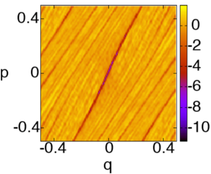
(a) (b)

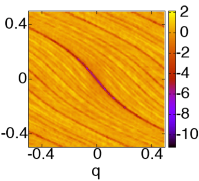
Figure 1: First subleading eigenfunctions of the (a) Perron-Frobenius- and (b) Koopman operator for the perturbed cat map. The Ulam matrix has size $2^{14}\times 2^{14}$.

Figure 1 shows the numerically computed second eigenfunctions of the Perron-Frobenius and Koopman operators with the Ulam discretization. They are striated along the unstable and stable manifolds respectively, that emanate from the fixed point at the origin.

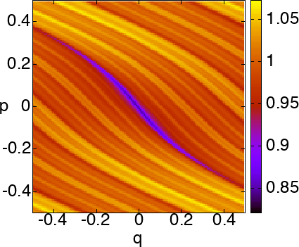
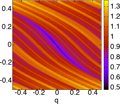
(a) (b) (c)

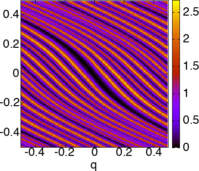
Figure 2: The phase-space distribution ($2^{14}$ points, each averaged over $10^{4}$ trajectories) of (a) the finite-time Lyapunov exponents, (b) the integrated kinetic energy, (c) the downstream observable $q^{2}(f^{t}(x))$ of the perturbed cat map, all having the $x=(q,p)$ coordinates as initial points of the trajectory $x\rightarrow f^{t}(x)$. The map is iterated until time $t=15$ in (a)-(b), $t=5$ in (c).

On the other hand, Figs. 2-3 illustrate the behavior of the numerically computed finite-time fields of three distinct observables, namely the stability exponent stemming from the Jacobian Eq. 10, the average kinetic energy $\overline{K}^{t}(x)=\frac{1}{2t}\int_{0}^{t}d\tau p^{2}(f^{\tau}(x))$, and the observable $q^{2}(x)$, which is both pushed forward as $q^{2}(f^{t}(x))$, and pulled back as $q^{2}(f^{-t}(x))$. The fields portrayed in the figures are obtained by iterating some $10^{8}$ randomly chosen, uniformly distributed initial conditions until a certain time $t$ before relaxation.

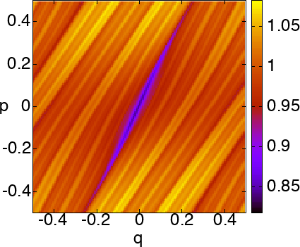
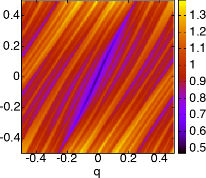
(a) (b) (c)

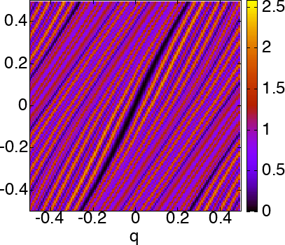
Figure 3: The phase-space distribution ($2^{14}$ points, each averaged over $10^{4}$ trajectories) of (a) the finite-time Lyapunov exponents, (b) the integrated kinetic energy, (c) the upstream observable $q^{2}(f^{-t}(x))$, of the perturbed cat map, all having the $x=(q,p)$ coordinates as final points of the trajectory $f^{-t}(x)\rightarrow x$. The map is iterated until time $t=15$ in (a)-(b), $t=5$ in (c).

The two integrated observables exhibit finite-time phase space distributions that share the features of the second eigenfunction of the Koopman operator (Fig. 1(b)) when pinned by the initial points $x_{0}$ of the trajectory $x_{0}\rightarrow f^{t}(x_{0})$ (Fig. 2(a)-(b)), as predicted by Eq. 7. Conversely, they both follow the behavior of the second eigenfunction of the Perron-Frobenius operator (Fig. 1(a)) when pinned by the final point of the same trajectory (Fig. 3(a)-(b)), as expected from Eq. 8. The third, instantaneous observable meets the predictions when downstream as $q^{2}(f^{t}(x_{0}))$ vs. $x_{0}$ (Eq. 7 and Fig. 2(c)) and upstream as $q^{2}(f^{-t}(x_{0}))$ vs. $x_{0}$ (Eq. 8 and Fig. 3(c)). It is noted that the relevant time scale changes from the Lagrangian averages ($t\simeq 15$) to the field $q^{2}(f^{t}(x))$ ($t\simeq 5$), since the coefficient $\int a(x)\phi_{1}(x)\,dx$ in the expansion Eq. 7 becomes $\int A^{t}(x)\phi_{1}(x)\,dx$ for integrated observables, and likewise backwards in time.

3.2 Hamiltonian Hénon map with noise

The next model to test the theory on is the Hamiltonian Hénon map

$$f\left(\begin{array}[]{c}q\\ p\end{array}\right)=\left(\begin{array}[]{c}1-\alpha q^{2}+\beta p\\ q\end{array}\right)$$ (17)

with $\alpha=1.4$ and $\beta=-1$. This map has no dissipation, but it does allow escape to infinity from the neighborhood of the two fixed points: $x_{p}\simeq(-1.1,-1.89)$ is unstable (‘hyperbolic’) and generates a chaotic saddle through its stable and unstable manifolds, while $x_{c}\simeq(0.39,0.39)$ is marginally stable (‘center’), and surrounded by a tiny stability island. In order to ‘kick’ the dynamics out of the latter non-chaotic region and into the chaotic phase, weak noise is added to the map (Eq. 17) of an amplitude comparable to the size of the stability island per unit time. Strictly speaking, the non-hyperbolicity of the resulting noisy system should introduce a continuous component in the spectrum of the transport operators and thus break the assumption of a solely discrete spectrum. However, if we investigate timescales of the order of or shorter than the (inverse) escape rate from the chaotic saddle, when the discrete part of the spectrum is non-negligible, the contribution of the continuous part of the spectrum may be ignored, due to the smallness of the stability island. Because the system admits escape and the first eigenfunction $\phi_{0}$ ($\varphi_{0}$) of ${\cal L}_{t}$ (${\cal L}^{\dagger}_{t}$) is non-uniform, the phase-space distributions of the pushed-forward, pulled-back or integrated observables for intermediate time scales are determined by the ratio of the second to the first eigenfunction of the evolution operator.

The predictions Eq. 7 and Eq. 8 are tested for two observables, that is the finite-time stability exponent and the diffusivity $\hat{D}^{t}(x)=\frac{1}{t}\int^{t}d\tau\,[q^{2}(f^{\tau}(x))+p^{2}(f^{\tau}(x))]$.

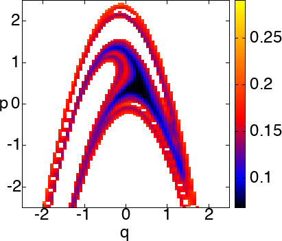
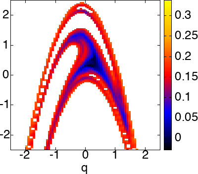
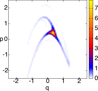
(a) (b) (c)
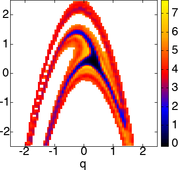
(d)      (e)

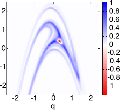
Figure 4: Phase-space distributions ($2^{14}$ points, each averaged over $10^{4}$ trajectories) of integrated oservables of the Hénon map with white, Gaussian noise of amplitude $\Delta=10^{-3}$, pinned by the initial points, after $t=10$ iterations of the map: (a) diffusivity; (b): finite-time Lyapunov exponents. (c) Ratio of the first subleading- (in (e)) to the leading (in (d)) eigenfunctions of the Koopman operator for the same noisy map, approximated with the Ulam method on a matrix of size $2^{14}\times 2^{14}$.

The density plots in Figure 4 corroborate the expectations for the field distributions of the two integrated observables to be supported on the stable manifold of the map when pinned by the initial points of the iteration $x_{0}\rightarrow f^{t}(x_{0})$ plus weak noise, and to mimic the density profile of the ratio between the second and the first eigenfunction of the Koopman operator.

On the other hand, the field distributions of the same observables pinned by the final points of each phase-space trajectory $f^{-t}(x_{0})\rightarrow x_{0}$ plus weak noise are supported on the unstable manifold of the map (Fig. 5), and behave similarly to the ratio of the second to the first eigenfunction of the Perron-Frobenius operator. In both ‘forward’ and ‘backward’ pictures, the strongly chaotic phase (in orange) is distinguishable from the non-hyperbolic, weakly chaotic phase (in blue) of a three-lobed shape with tapered ends, due to a period-three unstable periodic orbit that rules the dynamics just outside the stability island.

The white color in Figs. 4-5(a)(b) represents the region of the phase space where forward (Fig. 5) or backward (Fig. 4) trajectories escape from the domain examined before the time $t$ of integration, and thus it is not part of the field distributions. In Figs. 4-5(c), instead, the ratio between the eigenfunctions is not defined in the blank region, where the leading eigenfunction vanishes. The density plots of the leading- and subleading eigenfunctions of the transport operators (Figs. 4-5(d)(e)) taken separately, bear significant differences from the fields of the observables: the first eigenfunctions clearly describe a longer timescale than that of the field distributions, at which noisy trajectories have mostly left the hyperbolic region, while they only survive in and around the stability island; the second eigenfunctions alone are more resemblant of the finite-time fields, except they are suppressed on a ring around the stability island, a feature that does not have a kin in the distributions of the observables.

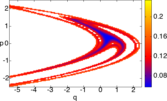
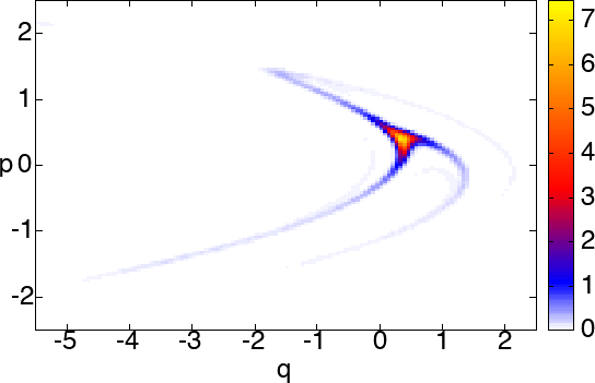
(a)      (b)
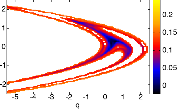
(c)
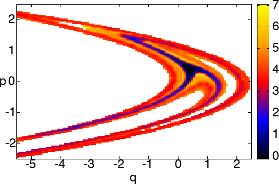
(d)      (e)

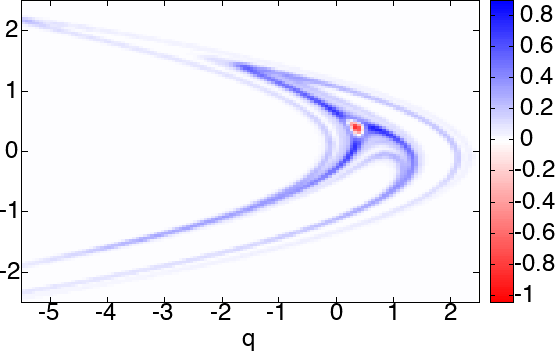
Figure 5: Phase-space distributions ($2^{14}$ points, each averaged over $10^{4}$ trajectories) of integrated oservables of the Hénon map with white, Gaussian noise of amplitude $\Delta=10^{-3}$, pinned by the final points, after $t=10$ iterations of the map: (a) diffusivity; (b): finite-time Lyapunov exponents. (c) Ratio of the first subleading- (in (e)) to the leading (in (d)) eigenfunctions of the Perron-Frobenius operator for the same noisy map, approximated with the Ulam method on a matrix of size $2^{14}\times 2^{14}$.

3.3 Discussion

Time-dependent phase-space distributions of observables advected by a chaotic dynamical system and before relaxation to statistical equilibrium exhibit universal features, determined by the first two eigenfunctions of the Perron-Frobenius or Koopman transport operators. This result follows from truncating the expansion of a pushed-forward or pulled-back chaotic field in terms of the eigenfunctions of the transport operators, whose spectrum is assumed discrete and with a spectral gap, meaning an exponential decay of correlations.

The theory is validated on two-dimensional models of chaos, but its implications go as far as the applicability of the Koopman treatment to problems of fluid dynamics (e.g. passive scalars [30], chaotic mixing [28], and turbulent aerosols [3]), neuronal networks, weather science, and time-series analysis in general, while it may serve as a valuable complement for those interested in Lagrangian coherent structures [17, 12], almost-invariant sets [14], or convective modes [4, 15].

As conveyed by the numerical tests on the Hamiltonian Hénon map, the theory presented here may not necessarily be restricted to hyperbolic systems, but rather extend to (noisy) mixed dynamics, when concerned with timescales that only involve the discrete part of the transport operator spectrum.

On the other hand, the present treatment is limited to $i)$ systems whose densities and fields are Lebesgue integrable at all times, unlike for example noiseless strange attractors, and $ii)$ featuring a real-valued second eigenvalue and eigenfunction for the transport operators. If instead the second eigenvalue is complex, decay of correlations and convergence to the (conditionally) invariant densities are not monotonic but oscillating, and one can show that the field profile stemming from the leading nontrivial terms in the expansions Eq. 7 and Eq. 8 gets to depend on the choice of the observable, when the latter is real valued. However, the universal behavior described here may still be recovered when $a(f^{t}(x))$ or its Lagrangian average are sampled over a longer time scale than that of the oscillation of the correlation decay. A more comprehensive theory addressing this phenomenology is already in the works and will be the object of a future report.

References

- [1] L. Alonso, J. A. Méndez-Bermúdez, A. González-Meléndrez, and Y. Moreno. Weighted random-geometric and random-rectangular graphs: spectral and eigenfunction properties of the adjacency matrix. Journal of Complex Networks, 6:753, 2018.
- [2] V. I. Arnold and A. Avez. Ergodic Problems of Classical Mechanics. Benjiamin, New York, 1968.
- [3] J. Bec, K. Gustavsson, and B. Mehlig. Statistical models for the dynamics of heavy particles in turbulence. Annual Review of Fluid Mechanics, 56:189, 2024.
- [4] C. Blachut and S. Balasuriya. Convective modes reveal the incoherence of the Southern Polar Vortex. Scientific Reports, 14:966, 2024.
- [5] M. Blank, G. Keller, and C. Liverani. Ruelle-Perron-Frobenius spectrum for Anosov maps. Nonlinearity, 15:1905, 2002.
- [6] E. M. Bollt and S. D. Ross. Is the finite-time Lyapunov exponent field a Koopman eigenfunction? Mathematics, 9:2731, 2021.
- [7] O. Bratteli and P. Jorgensen. The Transfer Operator and Perron-Frobenius Theory. Birkäuser, Basel, 2002.
- [8] P. Cvitanović, R. Artuso, R. Mainieri, G. Tanner, and G. Vattay. Chaos: Classical and Quantum. Niels Bohr Institute, Copenhagen, 2020.
- [9] P. Cvitanović and D. Lippolis. Knowing when to stop: how noise frees us from determinism. AIP Conference Proceedings, 1468:82, 2012.
- [10] R. M. D’Souza, M. di Bernardo, and Y.-Y. Liu. Controlling complex networks with complex nodes. Nature Reviews Physics, 5:250, 2023.
- [11] L. Ermann and D. L. Shepelyansky. The Arnold cat map, the Ulam method, and time reversal. Physica D, 241:514, 2012.
- [12] H. Aref et al. Frontiers of chaotic advection. Reviews of Modern Physics, 89:025007, 2017.
- [13] G. Froyland. On Ulam approximation of the isolated spectrum and eigenfunctions of hyperbolic maps. Discrete & Continuous Dynamical Systems, 17:671, 2007.
- [14] G. Froyland. Unwrapping eigenfunctions to discover the geometry of almost-invariant sets in hyperbolic maps. Physica D, 237:840, 2008.
- [15] G. Froyland, D. Giannakis, B. R. Lintner, M. Pike, and J. Slawinska. Spectral analysis of climate dynamics with operator-theoretic approaches. Nature Communications, 12(1):6570, 2021.
- [16] P. Gaspard. Chaos, Scattering, and Statistical Mechanics. Cambridge University Press, Cambridge, 1999.
- [17] G. Haller. Lagrangian coherent structures. Annual Review of Fluid Mechanics, 47:137, 2015.
- [18] S. C. Kapfer and W. Krauth. Irreversible local Markov chains with rapid convergence towards equilibrium. Physical Review Letters, 119:240603, 2017.
- [19] S. Klus, F. Nüske, S. Peitz, J.-H. Niemann, C. Clementi, and C. Schütte. Data-driven approximation of the Koopman generator: Model reduction, system identification, and control. Physica D, 406:132416, 2020.
- [20] M. L. Kringelbach and G. Deco. Brain states and transitions: Insights from computational neuroscience. Cell Reports, 32(10):108128, 2020.
- [21] T.-Y. Li. Finite approximation for the Perron-Frobenius operator, a solution to Ulam’s conjecture. Journal of Approximation Theory, 17:177, 1976.
- [22] D. Lippolis. Thermodynamics of chaotic relaxation processes. In preparation, February 2024.
- [23] Z. Lu and O. Raz. Nonequilibrium thermodynamics of the Markovian Mpemba effect and its inverse. Proceedings of the National Academy of Sciences of the United States of America, 114:5083, 2017.
- [24] C. C. Maiocchi, V. Lucarini, and A. Gritsun. Decomposing the dynamics of the Lorenz 1963 model using unstable periodic orbits: Averages, transitions, and quasi-invariant sets. Chaos, 32:033129, 2022.
- [25] R. Mohr and I. Mezić. Applied Koopmanism. Chaos, 22:047510, 2012.
- [26] H. Risken. The Fokker-Planck Equation. Springer, Berlin, 1996.
- [27] A. N. Souza. Transforming butterflies into graphs: Statistics of chaotic and turbulent systems. arXiv.2304.03362, 2023.
- [28] J.-L. Thiffeault. Scalar decay in chaotic mixing. Lecture Notes in Physics, 744:3, 2007.
- [29] S. M. Ulam. A Collection of Mathematical Problems. Interscience, New york, 1960.
- [30] Z. Warhaft. Passive scalars in turbulent flows. Annual Review of Fluid Mechanics, 32:203, 2000.
- [31] K. Yoshida, H. Yoshino, A. Shudo, and D. Lippolis. Eigenfunctions of the Perron–Frobenius operator and the finite-time Lyapunov exponents in uniformly hyperbolic area-preserving maps. Journal of Physics A: Mathematical and Theoretical, 54:285701, 2021.