Inexact and Implementable Accelerated Newton Proximal Extragradient Method for Convex Optimization

Abstract

In this paper, we investigate the convergence behavior of the Accelerated Newton Proximal Extragradient (A-NPE) method[36] when employing inexact Hessian information. The exact A-NPE method was the pioneer near-optimal second-order approach, exhibiting an oracle complexity of $\tilde{O}(\epsilon^{-2/7})$ for convex optimization. Despite its theoretical optimality, there has been insufficient attention given to the study of its inexact version and efficient implementation. We introduce the inexact A-NPE method (IA-NPE), which is shown to maintain the near-optimal oracle complexity. In particular, we design a dynamic approach to balance the computational cost of constructing the Hessian matrix and the progress of the convergence. Moreover, we show the robustness of the line-search procedure, which is a subroutine in IA-NPE, in the face of the inexactness of the Hessian. These nice properties enable the implementation of highly effective machine learning techniques like sub-sampling and various heuristics in the method. Extensive numerical results illustrate that IA-NPE compares favorably with state-of-the-art second-order methods, including Newton’s method with cubic regularization and Trust-Region methods.

1 Introduction

In this paper, we consider a generic unconstrained optimization problem as follows:

$$\min_{x\in\mathbb{R}^{d}}\ f(x):=g(x)+h(x),$$ (1.1)

where $f$ is bounded below by $f^{*}>-\infty$, $g$ is convex and twice continuously differentiable with Lipschitz continuous Hessian, $h$ is convex and Lipshitz continuous but possibly non-differentiable.

From a theoretical standpoint, second-order methods are preferable for their ability to address ill-conditioned problems and exhibit a better oracle complexity. In the realm of convex optimization, several variations of prominent second-order methods stand out. Noteworthy examples include the trust-region method (TR) [25], the cubic regularized Newton method (CR) [38], and the gradient regularized Newton method (GR) [17, 35].

Intriguingly, a historical review of accelerated second-order methods unveils their evolution over time. Nesterov [37] pioneered the field by proposing the initial accelerated second-order method, which improved the original version [38]. This rate of acceleration was improved by Monteiro and Svaiter [36], who introduced the A-NPE method, achieving an oracle complexity of $\tilde{O}(\epsilon^{-2/7})$. However, it’s worth noting that their algorithm necessitates a search procedure in each iteration to determine the suitable step size, adding extra logarithmic complexity. In recent years, Arjevani et al. [5] established a lower bound of $O(\epsilon^{-2/3p+1})$ for $p$-th order algorithms, highlighting that the A-NPE method happens to be nearly optimal up to a logarithmic factor. This observation has reignited interest in the A-NPE method. Simultaneously, researchers worldwide have independently extended the A-NPE method to accommodate higher-order information of objective functions. Three distinct groups[19] demonstrated that the modified method achieves an oracle complexity of $\tilde{O}(\epsilon^{-2/3p+1})$, albeit still relying on a search procedure for the appropriate step size. Remarkably, a composite structure is allowed in the higher order A-NPE method [24]. Recently, Kovalev and Gasnikov [28] and Carmon et al. [11] successfully eliminated the logarithmic factor in the complexity bound, making the A-NPE method a truly optimal algorithm. This marks a significant theoretical breakthrough in the field.

Despite the notable theoretical achievements, it’s crucial to acknowledge that the optimal complexity of the A-NPE method relies on exact Hessian information of the objective function, an impractical requirement in large-scale scenarios. In the realm of large-scale problems, the per-iteration computational complexity of second-order methods can become prohibitively expensive, primarily due to operations involving the Hessian. Addressing this challenge requires an examination of the convergence behavior when the Hessian is inexact.

In contrast with standard second-order methods, the A-NPE method introduces an additional layer of complexity by requiring the identification of a suitable step size in every iteration, a parameter not known in advance. This necessitates a search procedure in each iteration, and a good implementation of such a procedure is pivotal to the algorithm’s performance. To the best of our knowledge, most of the research on the A-NPE method focuses on the theoretical side, the only implementation by Carmon et al. [11] depends on exact Hessian information to derive the oracle complexity of $O(\epsilon^{-2/7})$, making it less practical for large-scale setting. (They also provide a CG routine to solve the subproblem, which fails to preserve the optimal oracle complexity.) This motivates us to analyze how the inexactness of the Hessian affects the search procedure. The challenge lies in proposing a robust algorithm that maintains theoretical complexity while being compatible with certain numerical heuristics.

Utilizing inexact Hessians is a widely employed technique to enhance the practical performance of second-order methods, demonstrating advantage from both theoretical and practical perspectives. The research focus is on designing algorithms using stochastic approximations to the Hessian. Various stochastic second-order methods have emerged, including but not limited to stochastic quasi-Newton methods [10, 43, 46], stochastic cubic regularized Newton methods [34, 45, 47], randomized cubic regularization methods [16], stochastic trust-region methods [7], random subspace Newton methods [21], Hessian sketching methods [6, 22, 30, 31, 40, 41], sub-sampling methods [3, 8, 9, 18, 29, 32, 33, 42, 48, 50].

Among the extensive literature, articles on inexact accelerated second-order methods are the most related to our study. Ghadimi et al. [20] proposed an accelerated cubic regularized Newton method with an inexact Hessian, while Ye et al. [51] applied Nesterov’s acceleration to enhance the approximate Newton method, both demonstrating favorable numerical performance. Song et al. [44] explored an accelerated inexact proximal cubic regularized Newton method with a complexity of $O(\epsilon^{-1/3})$ in the expectation sense. Chen et al. [14] and Kamzolov et al. [26] investigated the accelerated adaptive cubic regularized Newton method, showcasing the use of sub-sampling and quasi-Newton methods to approximate the Hessian within this framework, both yielding a complexity of $O(\epsilon^{-1/3})$ and promising numerical results. Antonakopoulos et al. [4] proposed a noise-adaptive accelerated second-order method with a universal global rate that adapts to the oracle’s variance. Agafonov et al. [1] introduced an accelerated inexact tensor method, demonstrating a complexity of $O(\epsilon^{-1/p+1})$ with access to the $p$-th order derivative. In recent work, Agafonov et al. [2] proposed a second-order method with stochastic gradient and Hessian, proving its tight convergence bound with respect to the variance of the gradient and the Hessian. However, none of these inexact methods achieve near-optimal oracle complexity $\tilde{O}(\epsilon^{-2/7})$ for second-order methods.

In this paper, we propose the inexact Accelerated Newton Proximal Extra-gradient (IA-NPE) method, where an adaptive procedure is designed to determine the inexactness of the Hessian. In particular, we allow a relatively large error of the Hessian at the beginning of the algorithm to reduce the cost of constructing the Hessian matrix. Note that the inexactness of the Hessian could affect the solution quality to the subproblem that appears in the main loop of the algorithm as well as the line search subroutine. Through meticulous analysis, we show that the near-optimal oracle complexity of $\tilde{O}(\epsilon^{-2/7})$ still holds for IA-NPE. We discuss the adaptability of techniques such as Newton sketch and sub-sampling within the IA-NPE method. Furthermore, we illustrate that numerous heuristics can be seamlessly integrated into the method, enhancing the practical performance of the algorithm. We present extensive numerical experiments focused on logistic regression problems. The results showcase that the IA-NPE method performs comparably to mainstream algorithms in the context of machine learning problems.

The rest of the paper is organized as follows. In section 2, we introduce some basic definitions and assumptions required in the paper. In section 3, we present the IA-NPE method in Algorithm 1 with its auxiliary search procedure in Algorithm 2. In section 4, we discuss how the inexactness of the Hessian information affects the auxiliary procedure and give a complexity analysis. In section 5, we analyze the overall complexity of the IA-NPE method. In section 6 and section 7, we demonstrate the applicability of modern machine-learning techniques to our algorithm and present promising results from numerical experiments.

2 Preliminaries

In this section, we introduce the basic definitions and assumptions used in the paper. Denote the standard Euclidean norm in space $\mathbb{R}^{d}$ by $\|\cdot\|$. For a operator $A:\mathbb{R}^{d}\rightarrow\mathbb{R}^{d}$, its norm is defined as

$$\|A\|=\sup\{\|Ax\|:\|x\|\leq 1,\ x\in\mathbb{R}^{d}\}.$$

Throughout this paper, we refer to the following definition of $\epsilon$-optimality.

Definition 2.1.

Given $\epsilon>0$, $x\in\mathbb{R}^{d}$ is said to be an $\epsilon$-optimal solution to problem (1.1), if

$$f(x)-f^{*}\leq O(\epsilon),$$ (2.1)

We can terminate the algorithm when we get points with such $\epsilon$-optimality.

Now we make some assumptions about the objective function.

Assumption 2.1.

The components $g$ and $h$ in (1.1) satisfy the following:

• $g$ and $h$ are proper closed convex functions.

• $g$ is twice continuously differentiable, the Hessian of $g$ is $L_{2}$-Lipschitz, i.e.,

  $$\|\nabla^{2}g(x)-\nabla^{2}g(y)\|\leq L_{2}\|x-y\|,\ \forall x,y\in\mathbb{R}^{d}.$$ (2.2)

• $h$ is $L^{\prime}$-Lipschitz continuous, i.e.,

  $$|h(x)-h(y)|\leq L^{\prime}\|x-y\|,\ \forall x,y\in\mathbb{R}^{d}.$$ (2.3)

Since our objective function concludes a non-differentiable part, we introduce the $\epsilon$-subdifferential of a proper closed convex function, whose basic properties are analyzed in Monteiro and Svaiter [36, Section 2].

Definition 2.2.

For $\epsilon\geq 0$, the $\epsilon$-subdifferential of a proper closed convex function $h:\mathbb{R}^{d}\to\mathbb{R}\cup\{+\infty\}$ is the operator $\partial_{\epsilon}h:\mathbb{R}^{d}\rightrightarrows\mathbb{R}^{d}$

$$\partial_{\epsilon}h(x)=\left\{v\in\mathbb{R}^{d}:h(y)\geq h(x)+\langle y-x,v\rangle-\epsilon,\ \forall y\in\mathbb{R}^{d}\right\},\ x\in\mathbb{R}^{d}.$$ (2.4)

Regarding the smooth component, when the dimension of the problem is large, approximate Hessian is often used to reduce the computational cost. We consider the approximation as introduced in the following definition.

Definition 2.3.

The $\delta$-inexact second-order approximation of $g$ at $x$ is

$$g_{x,\delta}(y):=g({x})+\langle\nabla g({x}),y-{x}\rangle+\frac{1}{2}\langle y-{x},H\left(x\right)\left(y-x\right)\rangle$$ (2.5)

where $H(\cdot)$ satisfies $\|H({x})-\nabla^{2}g({x})\|<\delta$ and $H(x)\succeq 0$.

Indeed, the above approximate Hessian can be constructed by various techniques, we will discuss this in section 6.

3 Overview of the IA-NPE Method

3.1 The IA-NPE Method and the Approximate Solution to the Subproblem

Algorithm 1 The IA-NPE Method

  Initialization: $x_{0},y_{0}\in\mathbb{R}^{d}$, $A_{0}=0$, $C,\bar{\rho},\bar{\epsilon},\delta_{-1}>0,\delta_{\max}>\delta_{-1}$, $\gamma>1$, and $0<\sigma_{l}<\sigma_{u}<1,0<\hat{\sigma}<1$ with

$$\hat{\sigma}+\sigma_{u}<1,\quad\sigma_{l}(1+\hat{\sigma})<\sigma_{u}(1-\hat{\sigma}),\quad\tilde{\sigma}:=C+\sigma_{u}+\hat{\sigma}<1.$$

  for $k=0,1,2,\cdots$ do

      Set $\delta_{k}=\min\left\{\gamma\delta_{k-1},\delta_{\max}\right\}$, $\lambda_{k+1}=\frac{C}{\delta_{k}}$, construct the approximate Hessian $H(\cdot)$;

      Compute $(\tilde{y}_{k+1},u_{k+1},\epsilon_{k+1})\in\operatorname{ANS}_{\hat{\sigma},\delta_{k}}(\lambda_{k+1},\tilde{x}_{k})$;

      while $\lambda_{k+1}\|\tilde{y}_{k+1}-\tilde{x}_{k}\|<\frac{2\sigma_{l}}{L_{2}}$ do

         Set $\delta_{k}=\delta_{k}/\gamma,\lambda_{k+1}=\frac{C}{\delta_{k}}$, update $H(\cdot)$ and $(\tilde{y}_{k+1},u_{k+1},\epsilon_{k+1})\in\operatorname{ANS}_{\hat{\sigma},\delta_{k}}(\lambda_{k+1},\tilde{x}_{k})$;

      end while

      if $\lambda_{k+1}\|\tilde{y}_{k+1}-\tilde{x}_{k}\|>\frac{2\sigma_{u}}{L_{2}}$ then

         Go to bisection search stage, compute $\lambda_{k+1}>0$ and $(\tilde{y}_{k+1},u_{k+1},\epsilon_{k+1})\in\operatorname{ANS}_{\hat{\sigma},\delta_{k}}(\lambda_{k+1},\tilde{x}_{k})$ with

$$\frac{2\sigma_{l}}{L_{2}}\leq\lambda_{k+1}\|\tilde{y}_{k+1}-\tilde{x}_{k}\|\leq\frac{2\sigma_{u}}{L_{2}},$$ (3.1)

      end ifwhere

$$\tilde{x}_{k} =\frac{A_{k}}{A_{k}+a_{k+1}}y_{k}+\frac{a_{k+1}}{A_{k}+a_{k+1}}x_{k},$$ (3.2)

$$a_{k+1} =\frac{\lambda_{k+1}+\sqrt{\lambda_{k+1}^{2}+4\lambda_{k+1}A_{k}}}{2}$$

      Set $y_{k+1}$ such that $f(y_{k+1})\leq f(\tilde{y}_{k+1})$ and

$$v_{k+1}=\nabla g(\tilde{y}_{k+1})+u_{k+1}-\nabla g_{\tilde{x}_{k},\delta}(\tilde{y}_{k+1}),$$

$$A_{k+1}=A_{k}+a_{k+1},$$

$$x_{k+1}=x_{k}-a_{k+1}v_{k+1}.$$

  end for

In this section, we first present the IA-NPE method as in Algorithm 1 with its line-search subroutine as in Algorithm 2 to find the stepsize. Recall that the A-NPE method[36] exploits the second-order information of the smooth part $g$ to solve a proximal operator inexactly in each iteration. Different from the original version, we introduce an inner loop to determine the inexactness level $\delta$ and construct the approximate Hessian $H(\cdot)$ accordingly. Given the $\delta$-inexact second-order approximation of $g$, the current solution $x$ and stepsize $\lambda>0$, the IA-NPE method solve the following subproblem in each iteration

$$y=\underset{u\in\mathbb{R}^{d}}{\mathop{\rm argmin}}\ g_{x,\delta}(u)+h(u)+\frac{1}{2\lambda}\|u-x\|^{2},$$ (3.3)

and the optimality condition of (3.3) is given by

$$v\in\left(\nabla g_{x,\delta}+\partial_{\epsilon}h\right)(y),\quad\lambda v+y-x=0.$$ (3.4)

In Algorithm 1, we solve (3.3) inexactly and get the following approximate Newton solution.

Definition 3.1.

Given $(\lambda,x)\in\mathbb{R}_{++}\times\mathbb{R}^{d}$, error tolerance $\delta>0$ and $\hat{\sigma}\geq 0$, the triple $(y,u,\epsilon)\in\mathbb{R}^{d}\times\mathbb{R}^{d}\times\mathbb{R}_{+}$ is called a $(\hat{\sigma},\delta)$-approximate Newton solution at $(\lambda,x)$ if

$$u\in(\nabla g_{x,\delta}+\partial_{\epsilon}h)(y),$$ (3.5)

$$\|\lambda u+y-x\|^{2}+2\lambda\epsilon\leq\hat{\sigma}^{2}\|y-x\|^{2}.$$ (3.6)

For simplicity, we denote the approximate solution in Definition 3.1 for short as

$$(y,u,v)\in\operatorname{ANS}_{\hat{\sigma},\delta}(\lambda,x).$$ (3.7)

The case $\delta=0$ in Definition 3.1 corresponds to a stricter approximate solution, which is based on the exact second-order information of the objective function.

Definition 3.2.

Given $(\lambda,x)\in\mathbb{R}_{++}\times\mathbb{R}^{d}$, error tolerance $\tilde{\sigma}\geq 0$, the triple $(y,v,\epsilon)\in\mathbb{R}^{d}\times\mathbb{R}^{d}\times\mathbb{R}_{+}$ is called a $\tilde{\sigma}$-approximate solution at $(\lambda,x)$ if

$$v\in(\nabla g_{x}+\partial_{\epsilon}h)(y),$$ (3.8)

$$\|\lambda v+y-x\|^{2}+2\lambda\epsilon\leq\tilde{\sigma}^{2}\|y-x\|^{2},$$ (3.9)

where $g_{x}(y)$ is the exact second-order expansion at $x$.

We will frequently use the properties of the above approximate solution in the convergence analysis. Moreover, we will later show that the two approximate solutions defined in Definition 3.1 and Definition 3.2 respectively are closely related.

Now we describe the line-search procedure in Algorithm 2, where the subscript is omitted for simplicity. Note that as the way $\tilde{x}$ is calculated in Algorithm 1, $\tilde{x}$ can be viewed as a continuous function of $\lambda$. Though the Hessian in Algorithm 1 is inexact, the bisection method as in [36] can still be adopted. Therefore, the problem considered in the line search procedure is as follows:
Line-search Problem: Given tolerance $\tilde{\sigma}\geq 0$, $\bar{\epsilon},\bar{\rho}>0$, bounds $\alpha_{+}>\alpha_{-}>0$, and a continuous curve $\tilde{x}:[0,\infty)\rightarrow\mathbb{R}^{d}$ satisfies certain smoothness condition. The problem is to find a stepsize $\lambda>0$ and a $\tilde{\sigma}$-approximate solution $(y_{\lambda},v_{\lambda},\epsilon_{\lambda})$ at $\left(\lambda,\tilde{x}\left(\lambda\right)\right)$ such that

$$\alpha_{-}\leq\lambda\|y_{\lambda}-\tilde{x}(\lambda)\|\leq\alpha_{+}.$$

Algorithm 2 The Bisection Search

  Input: Curve $\tilde{x}:[0,+\infty)\rightarrow\mathbb{R}$, right bracketing point $\lambda_{+}^{0}>0$, the inexactness parameter $\delta,C$, and bounds $\alpha_{+}\geq\alpha_{-}\geq 0$ satisfying

$$\alpha_{-}(1+\hat{\sigma})<\alpha_{+}(1-\hat{\sigma})$$ (3.10)

  Output: stepsize $\lambda>0$ and $(y_{\lambda},u_{\lambda},\epsilon_{\lambda})\in\operatorname{ANS}_{\hat{\sigma},\delta}(\lambda,\tilde{x}(\lambda))$ with $\alpha_{-}\leq\lambda\|y_{\lambda}-\tilde{x}(\lambda)\|\leq\alpha_{+}$.

  Bracketing Stage:

  compute $\lambda_{-}^{0}$ satisfies (4.13) and set $x_{-}^{0}=\tilde{x}(\lambda_{-}^{0})$, compute $(y_{-}^{0},u_{-}^{0},\epsilon_{-}^{0})\in\operatorname{ANS}_{\hat{\sigma},\delta}(\lambda_{-}^{0},x_{-}^{0})$;

  Bisection Stage: set $\lambda_{-}=\lambda_{-}^{0}$, $\lambda_{+}=\lambda_{+}^{0}$;

  for $k=1,2,\cdots$ do

      set $\lambda=\frac{\lambda_{-}+\lambda_{+}}{2}$, compute $(y_{\lambda},u_{\lambda},\epsilon_{\lambda})\in\operatorname{ANS}_{\hat{\sigma},\delta}(\lambda,\tilde{x}(\lambda))$ and set $v_{\lambda}=\nabla g(y_{\lambda})-\nabla g_{x_{\lambda},\delta}(y_{\lambda})+u_{\lambda}$;

      if $\lambda\|y_{\lambda}-\tilde{x}(\lambda)\|\in[\alpha_{-},\alpha_{+}]$ then

         stop and output the approximate solutions;

      else

         set

$$\left\{\begin{aligned} \lambda_{+}=\lambda,\ \lambda\|y_{\lambda}-\tilde{x}(\lambda)\|>\alpha_{+},\\ \lambda_{-}=\lambda,\ \lambda\|y_{\lambda}-\tilde{x}(\lambda)\|<\alpha_{-}.\end{aligned}\right.$$

      end if

  end for

The dominating cost of Algorithm 1 and Algorithm 2 will be computing the approximate Newton solution, thus the complexity is evaluated in terms of the number of oracles required to compute such an approximate solution during the whole minimization process.

Remark 3.1.

If there exists a $\tilde{\sigma}$-approximate solution $(y,v,\epsilon)$ at $(\lambda,x)$ with $\epsilon\leq\bar{\epsilon}$ and $\|v\|\leq\bar{\rho}$, where $\bar{\epsilon},\bar{\rho}$ are given tolerance, then we can directly terminate the algorithm and output $y$ as an approximate solution of (1.1). Therefore we always suppose there exists $\bar{\epsilon},\bar{\rho}\geq 0$ such that during the search procedure, the following holds for any $v$ and $\epsilon$:

$$\|v\|>\bar{\rho},\ \text{or }\epsilon>\bar{\epsilon}.$$ (3.11)

3.2 Alternative Representation of Approximate Newton Solution

Our analysis of the complexity of the algorithms depends on some existing results on the maximal monotone operator, thus we reformulate the approximate Newton solution and restate some important definitions in the context of maximal monotone operators. We put all proofs of the auxiliary technical results into the appendix for the coherence of the paper.

Note that as in Assumption 2.1, the minimization problem we consider can be viewed as a special case of the monotone inclusion problem with the following structure:

$$0\in\mathcal{T}(x):=(\mathcal{G}+\mathcal{H})(x).$$ (3.12)

Therefore, we make the following assumptions.

Assumption 3.1.

$\mathcal{G}:\mathbb{R}^{d}\to\mathbb{R}^{d}$ and $\mathcal{H}:\mathbb{R}^{d}\rightrightarrows\mathbb{R}^{d}$ satisfy the following:

• $\mathcal{H}$ is a maximal monotone operator, also, $\|y\|\leq L^{\prime}$ for any $x$ and $y\in\mathcal{H}(x)$.

• $\mathcal{G}$ is monotone and differentiable.

• $\mathcal{G}^{\prime}$ is $L_{2}$-Lipschitz continuous on $\mathbb{R}^{d}$.

Similar to Definition 3.2, we introduce the following approximate solutions of the proximal point iteration.

Definition 3.3.

Given $(\lambda,x)\in\mathbb{R}_{++}\times\mathbb{R}^{d}$, tolerance $\tilde{\sigma}\geq 0$, the triple $(y,v,\epsilon)$ is said to be a $\tilde{\sigma}$-approximate solution at $(\lambda,x)$ if

$$v\in\mathcal{T}^{\epsilon}(y),\ \|\lambda v+y-x\|^{2}+2\lambda\epsilon\leq\tilde{\sigma}^{2}\|y-x\|^{2}.$$ (3.13)

Here we also permit an error tolerance $\delta$ for $\mathcal{G}^{\prime}(\cdot)$, namely, we use an operator $\mathcal{P}(\cdot)$ with $\|\mathcal{G}^{\prime}(x)-\mathcal{P}(x)\|<\delta$ at all possible $x$ during the search procedure to approximate $\mathcal{G}^{\prime}(\cdot)$, we define the following inexact approximation and approximate Newton solution, corresponding to Definition 2.3 and Definition 3.1.

Definition 3.4.

For $x\in\mathbb{R}^{d}$, define the $\delta$-inexact first-order approximate of $\mathcal{T}_{x,\delta}:\mathbb{R}^{d}\to\mathbb{R}^{d}$ of $\mathcal{T}$ at $x$ as

$$\mathcal{T}_{x,\delta}(y)=\mathcal{G}_{x,\delta}(y)+\mathcal{H}(y),\ y\in\mathbb{R}^{d},$$ (3.14)

where $\mathcal{G}_{x,\delta}:\mathbb{R}^{d}\to\mathbb{R}^{d}$ is the $\delta$-inexact first-order approximate of $\mathcal{G}$ at $x$ given by:

$$\mathcal{G}_{x,\delta}(y)=\mathcal{G}(x)+\mathcal{P}(x)(y-x),$$ (3.15)

where $\|\mathcal{P}(x)-\mathcal{G}^{\prime}(x)\|<\delta$ and $\mathcal{P}$ should make $\mathcal{T}_{x,\delta}$ a maximal monotone operator.

Definition 3.5.

Given $(\lambda,x)\in\mathbb{R}_{++}\times\mathbb{R}^{d}$, error tolerance $\delta>0$ and $\hat{\sigma}\geq 0$, the triple $(y,u,\epsilon)\in\mathbb{R}^{d}\times\mathbb{R}^{d}\times\mathbb{R}_{+}$ is called a $(\hat{\sigma},\delta)$-approximate Newton solution at $(\lambda,x)$ if

$$u\in(\mathcal{G}_{x,\delta}+\mathcal{H}^{\epsilon})(y),$$ (3.16)

$$\|\lambda u+y-x\|^{2}+2\lambda\epsilon\leq\hat{\sigma}^{2}\|y-x\|^{2},$$ (3.17)

here $\mathcal{G}_{x,\delta}$ is the $\delta$-inexact first-order approximate of $\mathcal{G}$ at $x$ defined as in Definition 3.4.

With a slight abuse of the notation, we still adopt the notion as (3.7) in the monotone operator setting. The next proposition shows that a $\tilde{\sigma}$-approximate solution can be constructed with a $(\hat{\sigma},\delta)$-approximate Newton solution.

Proposition 3.1.

Let $(\lambda,x)\in\mathbb{R}_{++}\times\mathbb{R}^{d}$ and a $(\hat{\sigma},\delta)$-approximate Newton solution $(y,u,\epsilon)$ at $(\lambda,x)$ be given, and define $v:=\mathcal{G}(y)+u-\mathcal{G}_{x,\delta}(y)$.Then,

$$v\in(\mathcal{G}+\mathcal{H}^{\epsilon})(y)\subseteq\mathcal{T}^{\epsilon}(y),$$ (3.18)

$$\|\lambda v+y-x\|^{2}+2\lambda\epsilon\leq\left(\hat{\sigma}+\lambda\delta+\frac{L_{2}\lambda}{2}\left\|y-x\right\|\right)^{2}\|y-x\|^{2},$$ (3.19)

and

$$\|v\|\leq\frac{1}{\lambda}\left(1+\hat{\sigma}+\lambda\delta+\frac{L_{2}\lambda}{2}\left\|y-x\right\|\right)\|y-x\|,$$ (3.20)

$$\epsilon\leq\frac{\hat{\sigma}^{2}}{2\lambda}\|y-x\|^{2}.$$ (3.21)

4 Complexity of the Line-search Procedure

In this section, motivated from the idea in Monteiro and Svaiter [36, Section 7], we will show that the complexity of the line-search procedure is logarithmic in the problem parameters, although the exact Hessian information is unavailable.

4.1 Preliminary Results

For an approximate solution $(y,v,\epsilon)$ at $(\lambda,x)$ as in Definition 3.3, directly estimating the quantity $\lambda\|y-x\|$ may be difficult since the correspondence between $\lambda$ and the quantity is not single-valued. Thus it is necessary to find an approximation of the quantity that has a clear dependence of $\lambda$.

In order not to confuse the notations, consider a general maximal monotone operator $\mathcal{B}$, define for each $\lambda>0$,

$$y_{\mathcal{B}}(\lambda;x):=(I+\lambda\mathcal{B})^{-1}(x),\ \varphi_{\mathcal{B}}(\lambda,x):=\lambda\|y_{\mathcal{B}}(\lambda;x)-x\|.$$ (4.1)

Where $y_{\mathcal{B}}(\lambda,x)$ is the exact proximal point iteration from $x$ with stepsize $\lambda$.

Now we introduce some basic properties of $\varphi_{\mathcal{B}}$ that will be needed in the analysis. It can be shown that $\varphi_{\mathcal{B}}(\lambda;x)$ can serve as a good approximation to $\lambda\|y-x\|$.

Proposition 4.1.

(Monteiro and Svaiter [36, Proposition 7.1]) For every $x\in\mathbb{R}^{d}$, the following statements hold:
(a)$\lambda>0\to\varphi_{\mathcal{B}}(\lambda;x)$ is a continuous function;
(b)for every $0<\tilde{\lambda}\leq\lambda$,

$$\frac{\lambda}{\tilde{\lambda}}\varphi_{\mathcal{B}}(\tilde{\lambda};x)\leq\varphi_{\mathcal{B}}(\lambda;x)\leq\left(\frac{\lambda}{\tilde{\lambda}}\right)^{2}\varphi_{\mathcal{B}}(\tilde{\lambda};x)$$ (4.2)

The following result shows that the quantity $\lambda\|y-x\|$ can be well-approximated by $\varphi_{\mathcal{B}}(\lambda;x)$.

Proposition 4.2.

(Monteiro and Svaiter [36, Proposition 7.3]) Let $x\in\mathbb{R}^{d}$, $\lambda>0$ and $\tilde{\sigma}>0$ be given. If $(y,v,\epsilon)$ is a $\tilde{\sigma}$-approximate solution at $(\lambda,x)$,then

$$(1-\tilde{\sigma})\lambda\|y-x\|\leq\varphi_{\mathcal{B}}(\lambda;x)\leq(1+\tilde{\sigma})\lambda\|y-x\|.$$ (4.3)

4.2 Analysis of The Bracketing Points

The main goal of this section is to exploit the propositions of $\varphi_{\mathcal{B}}(\lambda;x)$ to find the bracketing points for the bisection procedure. Since we allow the derivative $\mathcal{G}^{\prime}$ of the smooth part to be inexact, we have to make the following assumption about the approximation.

Assumption 4.1.

The approximate operator $\mathcal{P}$ in Definition 3.4 has the Lipschitz coefficient $L_{2}$.

By the mechanism of the bisection procedure and the fact that $\lambda_{+}^{0}\delta=C$, we have the following observation.

Proposition 4.3.

During the search procedure, we always have $\lambda\delta\leq C$.

The next proposition illustrates the behavior of $\varphi_{\mathcal{B}}$ in terms of $x$, which helps find the bracketing points.

Proposition 4.4.

Given $\delta>0$ and let $x,\tilde{x}\in\mathbb{R}^{d}$ and $\lambda>0$ be given. Denote $\mathcal{B}:=\mathcal{T}_{x,\delta}$ and $\tilde{\mathcal{B}}:=\mathcal{T}_{\tilde{x},\delta}$, where $\mathcal{T}_{x,\delta}$ and $\mathcal{T}_{\tilde{x},\delta}$ are the $\delta$-inexact first-order approximation of $\mathcal{T}$ at $x$ and $\tilde{x}$. Then

$$\left|\varphi_{\mathcal{B}}\left(\lambda,x\right)-\varphi_{\tilde{\mathcal{B}}}\left(\lambda,\tilde{x}\right)\right|\leq(1+2C)\lambda\|\tilde{x}-x\|+L_{2}\lambda^{2}\|\tilde{x}-x\|^{2}+2L_{2}\lambda\|\tilde{x}-x\|\eta$$ (4.4)

where

$$\eta:=\min\left\{\varphi_{\mathcal{B}}\left(\lambda;x\right),\varphi_{\tilde{\mathcal{B}}}\left(\lambda;\tilde{x}\right)\right\}.$$ (4.5)

As a consequence,

$$\varphi_{\mathcal{B}}(\lambda,x)\leq(1+2C)\lambda\|\tilde{x}-x\|+L_{2}\lambda^{2}\|\tilde{x}-x\|^{2}+\left(2L_{2}\lambda\left\|\tilde{x}-x\right\|+1\right)\varphi_{\tilde{\mathcal{B}}}(\lambda;\tilde{x}).$$ (4.6)

With the help of the above propositions of $\varphi_{\mathcal{B}}$, we are now able to distinguish the bracketing points in the bisection procedure.

Proposition 4.5.

Let tolerance $\bar{v}>0$ and $\bar{\epsilon}>0$ , parameter $\hat{\sigma}\leq 0$ and $\alpha>0$ be given. Then for any

$$\lambda\geq\Lambda(\alpha):=\max\left\{\sqrt{\frac{\alpha}{\bar{v}}\left(1+\hat{\sigma}+C+\frac{L_{2}\alpha}{2}\right)},\left(\frac{\hat{\sigma}^{2}\alpha^{2}}{2\bar{\epsilon}}\right)^{\frac{1}{3}}\right\},$$ (4.7)

the $(\hat{\sigma},\delta)$-approximate Newton solution $(y,u,\epsilon)$ at $(\lambda,x)$ satisfies

$$\lambda\|y-x\|>\alpha$$

when $v=u-\mathcal{G}_{x,\delta}(y)+\mathcal{G}(y)$ such that (3.11) holds.

Proposition 4.6.

Let $(\lambda_{+}^{0},x_{+}^{0})\in\mathbb{R}_{++}\times\mathbb{R}^{d}$, and a $(\hat{\sigma},\delta)$-approximate Newton solution $(y_{+}^{0},u_{+}^{0},\epsilon_{+}^{0})$ at $(\lambda_{+}^{0},x_{+}^{0})$ be given. Then, for any scalar $\alpha$ and $\lambda_{-}^{0}$ with

$$0<\alpha\leq\lambda_{+}^{0}\|y_{+}^{0}-x_{+}^{0}\|,$$ (4.8)

$$\lambda_{-}^{0}\leq\frac{\alpha(1-\hat{\sigma})\lambda_{+}^{0}}{(1+\hat{\sigma})(1+2L_{2}\theta_{+}^{0})\lambda_{+}^{0}\|y_{+}^{0}-x_{+}^{0}\|+(1+2C)\theta_{+}^{0}+L_{2}(\theta_{+}^{0})^{2}},$$ (4.9)

$$\theta_{+}^{0}:=\lambda_{+}^{0}\|x_{+}^{0}-x_{-}^{0}\|$$

the $(\hat{\sigma},\delta)$-approximate Newton solution $(y_{-}^{0},u_{-}^{0},\epsilon_{-}^{0})$ at $(x_{-}^{0},\lambda_{-}^{0})$ satisfies

$$(1+\hat{\sigma})\lambda_{-}^{0}\leq(1-\hat{\sigma})\lambda_{+}^{0},$$ (4.10)

$$\lambda_{-}^{0}\|y_{-}^{0}-x_{-}^{0}\|\leq\alpha.$$ (4.11)

Note that in (4.9), $\lambda_{-}^{0}$ depends on $x_{-}^{0}$, which is unknown at current stage. To get rid of such dependence, suppose that the curve $x(\cdot)$ additionally satisfies that

$$\|\tilde{x}(s)-\tilde{x}(t)\|\leq\min\left\{\frac{M_{0}}{t}(s-t),M_{1}\left\|\tilde{x}(s)-\tilde{x}(0)\right\|\right\},\ 0<t\leq s$$ (4.12)

with some constant $M_{0},M_{1}>0$, then we can set the left bracketing point as the following instruction.

Corollary 4.1.

In Algorithm 2, if we set

$$\lambda_{-}^{0}=\frac{(1-\hat{\sigma})\alpha_{-}\lambda_{+}^{0}}{(1+\hat{\sigma})(1+2L_{2}\gamma_{0})\lambda_{+}^{0}\|y_{+}^{0}-x_{+}^{0}\|+(1+2C)\gamma_{0}+L_{2}(\gamma_{0})^{2}},$$ (4.13)

$$\gamma_{0}=M_{1}\lambda_{+}^{0}\|x_{+}^{0}-x(0)\|.$$

then the following condition holds:

$$\lambda_{+}^{0}\|y_{+}^{0}-x_{+}^{0}\|\geq\alpha_{+},\ \lambda_{-}^{0}\|y_{-}^{0}-x_{-}^{0}\|\leq\alpha_{-}.$$

4.3 Complexity of the Bisection Stage

In this section, with the bracketing points at hand, we are able to analyze the complexity of the bisection stage of Algorithm 2. We give the formal proof of Theorem 4.1 here to show how the propositions contribute to the final analysis.

Proposition 4.7.

Assume that $x_{*}\in\mathcal{T}^{-1}(0)=(\mathcal{G}+\mathcal{H})^{-1}(0)$, for any $\lambda>0$ and $x\in\mathbb{R}^{d}$, let $\mathcal{T}_{x,\delta}$ denotes the $\delta$-inexact first-order approximate of $\mathcal{T}$ at $x$, then there holds

$$\varphi_{\mathcal{T}_{x}}(\lambda;x)\leq\frac{2L^{\prime}\lambda^{2}}{1-C}+\frac{\lambda}{1-C}\|x-x_{*}\|+\frac{\lambda^{2}L_{2}}{1-C}\|x-x_{*}\|^{2},$$ (4.14)

where $L^{\prime}$ is the upper bound of $\mathcal{H}$ according to (3.12).

Theorem 4.1.

The bisection stage of Algorithm 2 makes at most

$$2+\log\left[C_{0}^{2}M_{0}\lambda_{+}^{0}\left(\frac{1+2C+L_{2}M_{0}\lambda_{+}^{0}+2\left(L_{2}+\frac{1}{M_{0}\lambda_{+}^{0}}\right)(1+\hat{\sigma})\alpha_{-}}{(1-\hat{\sigma})\alpha_{+}-(1+\hat{\sigma})\alpha_{-}}\right)\right]$$ (4.15)

oracle calls, where $\lambda_{+}^{0}$ is as in the definition in the framework above, and

$$C_{0}= \frac{(1+\hat{\sigma})(1+2L_{2}\gamma_{0})\left[2L^{\prime}\left(\lambda_{+}^{0}\right)^{2}+\lambda_{+}^{0}d\left(x_{+}^{0}\right)+\left(\lambda_{+}^{0}\right)^{2}L_{2}d\left(x_{+}^{0}\right)^{2}\right]}{(1-C)(1-\hat{\sigma})^{2}\alpha_{-}}$$ (4.16)

$$+\frac{\left[\left(1+2C\right)\gamma_{0}+L_{2}\left(\gamma_{0}\right)^{2}\right](1-C)(1-\hat{\sigma})}{(1-C)(1-\hat{\sigma})^{2}\alpha_{-}},$$

$\gamma_{0}$ is defined in (4.13) and $d(x_{+}^{0})$ denotes the distance of $x_{+}^{0}$ to $x_{*}$.

Proof First, we observe that the bracketing stage in Algorithm 2 makes one oracle call. By the mechanism of the bisection method, it follows that after $j$ bisection iterations,

$$\lambda_{+}-\lambda_{-}=\frac{1}{2^{j}}(\lambda_{+}^{0}-\lambda_{-}^{0})\leq\frac{1}{2^{j}}\lambda_{+}^{0},$$ (4.17)

and hence

$$j\leq\log\left(\frac{\lambda_{+}^{0}}{\lambda_{+}-\lambda_{-}}\right).$$ (4.18)

Assume now that the method doesn’t stop at the $j$-th bisection iteration. Then, the values of $\lambda_{-}$ and $\lambda_{+}$ of this iteration satisfy

$$\lambda_{+}\|y_{\lambda_{+}}-x(\lambda_{+})\|>\alpha_{+},\lambda_{-}\|y_{\lambda_{-}}-x(\lambda_{-})\|<\alpha_{-},$$ (4.19)

and let $x_{+}:=\tilde{x}(\lambda_{+})$, $x_{-}=\tilde{x}(\lambda_{-})$. Let $\mathcal{B}_{+}:=\mathcal{T}_{x_{+},\delta}$ and $\mathcal{B}_{-}:=\mathcal{T}_{x_{-},\delta}$. Applying Proposition 4.2 twice, one time with $\mathcal{B}=\mathcal{B}_{+},x=x_{+}$, and $(y,u,\epsilon)=(y_{+},u_{+},\epsilon_{+})$, and the other with $\mathcal{B}=\mathcal{B}_{-},x=x_{-}$, and $(y,u,\epsilon)=(y_{-},u_{-},\epsilon_{-})$, we conclude that

$$\varphi_{+}:=\varphi_{\mathcal{B}_{+}}(\lambda_{+};x_{+})>(1-\hat{\sigma})\alpha_{+},\ \varphi_{-}:=\varphi_{\mathcal{B}_{-}}(\lambda_{-};x_{-})<(1+\hat{\sigma})\alpha_{-}.$$ (4.20)

On the other hand, it follows from Proposition 4.1 with $\mathcal{B}=\mathcal{B}_{+},x=x_{+},\tilde{\lambda}=\lambda_{-}$ and $\lambda=\lambda_{+}$, Proposition 4.4 with $\lambda=\lambda_{-},x=x_{+}$ and $\tilde{x}=x_{-}$, that

$$\varphi_{+} =\varphi_{\mathcal{B}_{+}}(\lambda_{+};x_{+})\leq\left(\frac{\lambda_{+}}{\lambda_{-}}\right)^{2}\varphi_{\mathcal{B}_{+}}(\lambda_{-};x_{+})$$ (4.21)

$$\leq\left(\frac{\lambda_{+}}{\lambda_{-}}\right)^{2}\left[\left(1+2C\right)\theta+L_{2}\theta^{2}+\left(1+2L_{2}\theta\right)\varphi_{-}\right],$$ (4.22)

from the smoothness condition (4.12) we can conclude

$$\theta:=\lambda_{-}\|x_{+}-x_{-}\|\leq M_{0}(\lambda_{+}-\lambda_{-}),$$ (4.23)

given the property assumed for the curve $x(\cdot)$. Hence, we conclude that

$$\varphi_{+}-\varphi_{-}\leq \left(\frac{\lambda_{+}}{\lambda_{-}}\right)^{2}\theta(1+2C+L_{2}\theta+2L_{2}\varphi_{-})+\left[\left(\frac{\lambda_{+}}{\lambda_{-}}\right)^{2}-1\right]\varphi_{-}$$

$$\leq \left(\frac{\lambda_{+}^{0}}{\lambda_{-}^{0}}\right)^{2}M_{0}(1+2C+L_{2}M_{0}\lambda_{+}^{0}+2L_{2}\varphi_{-})(\lambda_{+}-\lambda_{-})$$

$$+\frac{\lambda_{+}+\lambda_{-}}{(\lambda_{-})^{2}}\varphi_{-}(\lambda_{+}-\lambda_{-})$$

$$\leq \left(\frac{\lambda_{+}^{0}}{\lambda_{-}^{0}}\right)^{2}M_{0}(1+2C+L_{2}M_{0}\lambda_{+}^{0}+2L_{2}\varphi_{-})(\lambda_{+}-\lambda_{-})$$

$$+2\frac{\lambda_{+}^{0}}{(\lambda_{-}^{0})^{2}}\varphi_{-}(\lambda_{+}-\lambda_{-})$$

$$= (\lambda_{+}-\lambda_{-})\left(\frac{\lambda_{+}^{0}}{\lambda_{-}^{0}}\right)^{2}M_{0}\left[1+2C+L_{2}M_{0}\lambda_{+}^{0}+2\left(L_{2}+\frac{1}{M_{0}\lambda_{+}^{0}}\right)\varphi_{-}\right].$$

Combining the latter inequality with (4.20), we then conclude that

$$\frac{1}{\lambda_{+}-\lambda_{-}}\leq\left(\frac{\lambda_{+}^{0}}{\lambda_{-}^{0}}\right)^{2}M_{0}\left(\frac{1+2C+L_{2}M_{0}\lambda_{+}^{0}+2\left(L_{2}+\frac{1}{M_{0}\lambda_{+}^{0}}\right)\left(1+\hat{\sigma}\right)\alpha_{-}}{\left(1-\hat{\sigma}\right)\alpha_{+}-\left(1+\hat{\sigma}\right)\alpha_{-}}\right).$$ (4.24)

We will now estimate the radio $\frac{\lambda_{+}^{0}}{\lambda_{-}^{0}}$. First note that Proposition 4.2 with $\lambda=\lambda_{+}^{0},x=x_{+}^{0},\mathcal{B}=\mathcal{T}_{x_{+}^{0},\delta}$ and $(y,u,\epsilon)=(y_{+}^{0},u_{+}^{0},\epsilon_{+}^{0})$, and Proposition 4.7 with $\lambda=\lambda_{+}^{0},x=x_{+}^{0}$ imply that

$$\lambda_{+}^{0}\|y_{+}^{0}-x_{+}^{0}\|\leq\frac{\varphi_{\mathcal{T}_{x_{+}^{0},\delta}}(\lambda_{+}^{0};x_{+}^{0})}{1-\hat{\sigma}}\leq\frac{2L^{\prime}(\lambda_{+}^{0})^{2}+\lambda_{+}^{0}d(x_{+}^{0})+(\lambda_{+}^{0})^{2}L_{2}d(x_{+}^{0})^{2}}{(1-C)(1-\hat{\sigma})}.$$

Then using the latter inequality together with the definition of $\lambda_{-}^{0}$ in the framework, we can imply that

$$\frac{\lambda_{+}^{0}}{\lambda_{-}^{0}}= \frac{(1+\hat{\sigma})(1+2L_{2}\gamma_{0})\lambda_{+}^{0}\|y_{+}^{0}-x_{+}^{0}\|+(1+2C)\gamma_{0}+L_{2}(\gamma_{0})^{2}}{(1-\hat{\sigma})\alpha_{-}}$$

$$\leq \frac{(1+\hat{\sigma})(1+2L_{2}\gamma_{0})\left[2L^{\prime}\left(\lambda_{+}^{0}\right)^{2}+\lambda_{+}^{0}d\left(x_{+}^{0}\right)+\left(\lambda_{+}^{0}\right)^{2}L_{2}d\left(x_{+}^{0}\right)^{2}\right]}{(1-C)(1-\hat{\sigma})^{2}\alpha_{-}}$$

$$+\frac{+\left[\left(1+2C\right)\gamma_{0}+L_{2}\left(\gamma_{0}\right)^{2}\right](1-C)(1-\hat{\sigma})}{(1-C)(1-\hat{\sigma})^{2}\alpha_{-}}.$$

Then we know

$$j\leq\log\left[C_{0}^{2}M_{0}\lambda_{+}^{0}\left(\frac{1+2C+L_{2}M_{0}\lambda_{+}^{0}+2\left(L_{2}+\frac{1}{M_{0}\lambda_{+}^{0}}\right)(1+\hat{\sigma})\frac{2\sigma_{l}}{L_{2}}}{(1-\hat{\sigma})\frac{2\sigma_{u}}{L_{2}}-(1+\hat{\sigma})\frac{2\sigma_{l}}{L_{2}}}\right)\right].$$ (4.25)

The result now follows from the above inequality. ∎Furthermore, by ignoring the parameters, the above complexity can be simplified.

Theorem 4.2.

Algorithm 2 makes at most

$$O\left(\max\left\{\log L_{2},\log d(x_{+}^{0}),\log M_{1},\log M_{0},\log L^{\prime},\log\frac{1}{\bar{\rho}},\log\frac{1}{\bar{\epsilon}}\right\}\right)$$ (4.26)

oracle calls to compute a stepsize $\lambda_{k+1}>0$ that solves the line-search problem at $k$-th iteration.

5 Complexity Analysis of the IA-NPE Method

5.1 Convergence of the main loop in Algorithm 1

To establish the convergence of the IA-NPE method, the first thing is to check the complexity of the while loop of Algorithm 1. Note that whenever $\lambda_{k+1}\|\tilde{y}_{k+1}-\tilde{x}_{k}\|\geq\frac{2\sigma_{l}}{L_{2}}$, the while loop will terminate, thus we come to the following lemma.

Lemma 5.1.

In the $k$-th iteration of Algorithm 1, the while loop will terminate after at most

$$\log_{\gamma}\frac{\delta_{\max}\Lambda\left(\frac{2\sigma_{l}}{L_{2}}\right)}{C}$$ (5.1)

oracle calls. Where $\Lambda(\cdot)$ is defined in (4.7).

We now recall the following proposition that guarantees the iteration complexity of $O(\epsilon^{-2/7})$ for the main loop of the large step A-NPE method[36].

Proposition 5.1.

There exists $0<\tilde{\sigma}<1$ such that for every iteration $k$,

$$v_{k+1}\in(\nabla g+\partial_{\epsilon_{k+1}}h)(\tilde{y}_{k+1})\subseteq\partial_{\epsilon_{k+1}}(g+h)(\tilde{y}_{k+1}),$$ (5.2)

$$\|\lambda_{k+1}v_{k+1}+\tilde{y}_{k+1}-\tilde{x}_{k}\|^{2}+2\lambda_{k+1}\epsilon_{k+1}\leq\tilde{\sigma}^{2}\|\tilde{y}_{k+1}-\tilde{x}_{k}\|^{2},$$ (5.3)

It now remains to check if there exists a constant $\tilde{\sigma}$ such that Proposition 5.1 holds for Algorithm 1. Luckily, when the error of the approximate Hessian is within $\delta_{k}$, such constant indeed exists and the error brought by the inexact Hessians can be controlled.

Lemma 5.2.

In each iteration $k$, suppose that

$$\|\nabla^{2}g(\tilde{x}_{k})-H(\tilde{x}_{k})\|\leq\delta_{k},$$ (5.4)

we have

$$v_{k+1}\in(\nabla g+\partial_{\epsilon_{k+1}}h)(\tilde{y}_{k+1})\subseteq\partial_{\epsilon_{k+1}}(g+h)(\tilde{y}_{k+1}),$$

$$\|\lambda_{k+1}v_{k+1}+\tilde{y}_{k+1}-\tilde{x}_{k}\|^{2}+2\lambda_{k+1}\epsilon_{k+1}\leq\tilde{\sigma}^{2}\|\tilde{y}_{k+1}-\tilde{x}_{k}\|^{2},$$ (5.5)

where $\tilde{\sigma}=\sigma_{u}+\hat{\sigma}+C$.

The proof of Lemma 5.2 is similar to the proof of Proposition 3.1, we omit it for simplicity. Now the convergence and the boundedness of the iterates can be guaranteed.

Theorem 5.1.

(Monteiro and Svaiter [36, Theorem 3.10, Theorem 6.4]) Let $X^{*}$ be the set of optimal solutions and $x^{*}$ be the projection of $x_{0}$ onto $X^{*}$, denote $d_{0}=\|x_{0}-x^{*}\|$, $\{x_{k}\},\{y_{k}\}$ are generated by Algorithm 1, then we have

$$\|x_{k}-x_{*}\|\leq d_{0},\ \|y_{k}-x^{*}\|\leq\left(\frac{2}{\sqrt{1-\tilde{\sigma}^{2}}}+1\right)d_{0},$$

$$f(y_{k+1})-f_{*}\leq\frac{3^{7/2}}{4\sqrt{2}}\frac{L_{2}d_{0}^{3}}{\sigma_{l}\sqrt{1-\tilde{\sigma}^{2}}}\frac{1}{k^{7/2}}$$

5.2 Total Complexity of the Algorithm

Now we are able to analyze the total complexity of Algorithm 1. We first note that the line-search stage in Algorithm 1 can be viewed as a special case of the problem we described in section 4, it corresponds to the case where $\mathcal{H}=\partial h,\mathcal{G}=\nabla g$, the first-order approximation $\mathcal{T}_{x,\delta}=\nabla g_{x,\delta}+\partial h$. The curve $\tilde{x}_{k}(\cdot)$ is calculated as in (3.2). We first show that the curve satisfies the smoothness condition (4.12) and the subdifferentiable set is bounded.

Lemma 5.3.

(Monteiro and Svaiter [36, Lemma 7.13]) The curve $\tilde{x}_{k}(\cdot)$ satisfies (4.12) with

$$M_{0}=\left(\frac{2}{\sqrt{1-\tilde{\sigma}^{2}}}+1\right)d_{0},\ M_{1}=1.$$ (5.6)

Lemma 5.4.

If $h$ has a Lipschitz coefficient $L^{\prime}$, then for any $\epsilon\geq 0$, $x\in\mathbb{R}^{d}$ and any $v\in\partial h_{\epsilon}(x)$, we have

$$\|v\|\leq L^{\prime}.$$ (5.7)

Now we can give the complete complexity result of Algorithm 1.

Theorem 5.2.

If in each iteration $k$

$$\|H(x_{k,\lambda})-\nabla^{2}g(x_{k,\lambda})\|\leq\delta_{k},$$ (5.8)

where $x_{k,\lambda}$ denotes all iterates during the line-search stage of the $k$-the iteration, then Algorithm 1 makes no more than

$$O\left(L_{2}d_{0}^{3}\epsilon^{-2/7}\max\left\{\left(\log L_{2}\right)^{2},\log d_{0},\log L^{\prime},\left(\log\left(1/\bar{\rho}\right)\right)^{2},\left(\log\left(1/\bar{\epsilon}\right)\right)^{2}\right\}\right)$$ (5.9)

oracle calls to find an approximate solution $y_{k}$ satisfies

$$f(y_{k})-f^{*}\leq\epsilon$$

or a $\tilde{\sigma}$-approximate solution $(y_{k},v_{k},\epsilon_{k})$ with

$$\|v_{k}\|\leq\bar{\rho},\ \epsilon_{k}\leq\bar{\epsilon}.$$

Proof This theorem is a direct consequence of Theorem 4.2, Lemma 5.1, Lemma 5.3, Theorem 5.1. ∎

6 Subroutines for Approximating the Hessian

In this section, we show that when the objective function in (1.1) has certain special structures, some techniques can be applied to approximate the Hessian of the smooth part. For example, when the dimension of the problem is high, we can use a subspace approximation to the Hessian. In addition, we can apply a sub-sampling technique when the objective function has a finite-sum structure. For the sub-sampling technique, we provide a formal analysis and show that the technique is compatible with the IA-NPE algorithm both theoretically and practically.

6.1 Subspace Approximation

Note that in Algorithm 1, we first determine the error of the inexact Hessian $\delta_{k}$ and then construct the approximate Hessian, when $\delta_{k}$ is relatively large, we can use the subspace approximation or the Newton sketch technique.

Take the Newton sketch technique as an example, when the square root of the Hessian of the objective function is easily computable, we can apply this technique. Let’s say an objective function with a structure of

$$f(x)=\sum_{i=1}^{n}f_{i}(a_{i}^{T}x),$$

the square root of the Hessian is $\nabla^{2}f(x)^{1/2}=\textbf{diag}\left(f_{i}^{\prime\prime}\left(a_{i}^{T}x\right)^{1/2}\right)A$, where $A$ denotes the data matrix.

Specifically, at every iteration, a random sketch matrix $S_{k}\in\mathbb{R}^{m\times d}$ is defined, where $m<d$. The approximate Hessian was defined to be

$$H(x):=\nabla^{2}g(x)^{1/2}S_{k}^{T}S_{k}\nabla^{2}g(x).$$ (6.1)

Theoretically, it is difficult to establish the relation between the error $\delta_{k}$ and the dimension $m$. However, we can dynamically increase the sketch dimension when the current error is seemingly larger than the pre-given inexactness $\delta_{k}$.

An inner loop to approximate the Hessian by sketching can be designed. We can start with a small dimension, construct the sketch Hessian, and check whether the left and right bracketing points are well-defined, specifically, we should check if

$$\lambda_{+}^{0}\|y_{+}^{0}-x_{+}^{0}\|\geq\alpha_{+},\ \lambda_{-}^{0}\|y_{-}^{0}-x_{-}^{0}\|\leq\alpha_{-}$$

holds in the bisection stage, if not, we can double the sketching dimension, i.e., we set $m\to 2m$ and construct the sketch Hessian again. Empirically, when the dimension approaches the effective dimension as in [31], which is usually less than $d$, we may ensure that we have a good approximate. Even in the worst case, when the dimension approaches $d$, the sketching Hessian will be a good approximation. Thus the inner loop at most has a logarithmic complexity.

6.2 Sub-Sampling Approximation

When objective function has the finite-sum structure

$$f(x)=\sum_{i=1}^{n}f_{i}(x),$$

the sub-sampling technique can help reduce the computational cost, we assume each component $f_{i}$ satisfies the following assumption.

Assumption 6.1.

Each $f_{j}(x)$ has a composite form $f_{j}(x)=g_{j}(x)+h_{j}(x)$, where the following conditions are assumed to hold:

• The objective function $f(x):=\frac{1}{n}\sum_{j=1}^{n}f_{j}(x)$ is convex, $g(x):=\frac{1}{n}\sum_{j=1}^{n}g_{j}(x)$ and $h(x):=\frac{1}{n}\sum_{j=1}^{n}h_{j}(x)$ are both proper closed convex functions.

• $g_{j}$ is twice continuously differentiable with its gradient and Hessian being Lipschitz continuous, i.e., there are $0<L_{1,g_{j}},L_{2,g_{j}}<\infty$ such that for any $x,y\in\mathbb{R}^{d}$

  $$\left\|\nabla g_{j}(x)-\nabla g_{j}(y)\right\|\leq \ L_{1,g_{j}}\left\|x-y\right\|,$$ (6.2)

  $$\left\|\nabla^{2}g_{j}(x)-\nabla^{2}g_{j}(y)\right\|\leq \ L_{2,g_{j}}\left\|x-y\right\|.$$ (6.3)

• $h_{j}$ is Lipschitz continuous, i.e., there exists $0<L_{h_{j}}<\infty$ such that for any $x,y\in\mathbb{R}^{d}$

  $$\left\|h_{j}(x)-h_{j}(y)\right\|\leq \ L_{h_{j}}\left\|x-y\right\|.$$ (6.4)

In the rest of the section, we define

$$L_{1}=\max_{1\leq j\leq n}L_{1,g_{j}},\ L_{2}=\max_{1\leq j\leq n}L_{2,g_{j}},\ L^{\prime}=\max_{1\leq j\leq n}L_{h_{j}}.$$

The following technical lemmas are mostly from Xu et al. [49] so we omit the proof here.

Let $\mathcal{S}$ and $\left|\mathcal{S}\right|$ denote the sample collection and its cardinality, $p_{i}=\textnormal{Prob}\left(\xi=i\right)$ denotes the probability that the index $i$ is chosen, and define

$$\tilde{H}(x)=\frac{1}{n\left|\mathcal{S}\right|}\sum_{j\in\mathcal{S}}\frac{1}{p_{j}}\nabla^{2}g_{j}(x).$$ (6.5)

When $n$ is very large, such random sampling can significantly reduce the per-iteration computational cost as $\left|\mathcal{S}\right|\ll n$.

One natural sampling scheme is to use the uniform sampling, i.e., $p_{i}=\frac{1}{n}$ for $i=1,2,\ldots,n$. There are other sampling schemes, we refer interested readers to [42, 48, 49].

The following lemmas reveal how many samples are required to get a sub-sampled Hessian within a given accuracy if the indices are sampled uniformly with replacement.

Lemma 6.1.

Suppose Assumption 2.1 holds and for $x\in\mathbb{R}^{d}$, $\tilde{H}(x)$ is constructed from (6.5) with $p_{j}=\frac{1}{n}$. When sample size

$$\left|\mathcal{S}\right|\geq\frac{16L_{1}^{2}}{\kappa^{2}}\log\left(\frac{2Nd}{\delta^{\prime}}\right)$$ (6.6)

for given $0<\kappa,\delta^{\prime}<1$. Then for any $N$ points $x_{i}\in\mathbb{R}^{d},i=1,\ldots,N$ we have

$$\textnormal{Prob}\left(\bigcup_{i=1}^{N}\left\{\left\|\tilde{H}(x_{i})-\nabla^{2}g(x_{i})\right\|\geq\kappa\right\}\right)<\delta^{\prime}.$$

In view Assumption 2.1 and the way we construct the sub-sampled Hessian matrices stated in (6.5), we have the following remark.

Remark 6.1.

The sub-sampled Hessian $\tilde{H}(x_{k})$ constructed by (6.5) with sample size satisfying (6.6) has the Lipschitz coefficient $L_{2}$.

The sub-sampled Hessian won’t be changed during the search procedure to preserve the Lipschitz continuity. We will specify the way of constructing the approximate Hessian $H(\cdot)$ in Algorithm 1.

Lemma 6.2.

Given the overall failure probability $\delta_{0}$, in the $k$-th iteration, if we set

$$\delta^{\prime}=O(\delta_{0}\epsilon^{2/7}),\ \kappa=\frac{\delta_{k}}{2},\ N=\max\left\{\log L_{2},\log d_{0},\log L^{\prime},\log\left(1/\bar{\rho}\right),\log\left(1/\bar{\epsilon}\right)\right\}$$ (6.7)

in (6.6) and set the approximate Hessian as

$$H(x)=\tilde{H}(x)+\frac{\delta_{k}}{2}I,$$ (6.8)

then

$$\|H(x_{k,\lambda})-\nabla^{2}g(x_{k,\lambda})\|\leq\delta_{k},\ H(x)\succeq 0$$ (6.9)

with probability $1-O(\delta_{0}\epsilon^{2/7})$.

To describe the convergence behavior of Algorithm 1 in terms of probability, we have the following equivalent result.

Theorem 6.1.

If we construct the approximate Hessian as instructed in Lemma 6.2, then when Algorithm 1 makes

$$O\left(L_{2}d_{0}^{3}\epsilon^{-2/7}\max\left\{\left(\log L_{2}\right)^{2},\log d_{0},\log L^{\prime},\left(\log\left(1/\bar{\rho}\right)\right)^{2},\left(\log\left(1/\bar{\epsilon}\right)\right)^{2}\right\}\right)$$

oracle calls, with probability $1-\delta_{0}$ we have an approximate solution $y_{T}$ with

$$f(y_{T})-f^{*}\leq O(\epsilon)$$

or we have a $\tilde{\sigma}$-approximate solution $(y_{T},v_{T},\epsilon_{T})$ with

$$\|v_{T}\|\leq\bar{\rho},\ \epsilon_{T}\leq\bar{\epsilon}.$$

7 Numerical Experiment

In this section, we present the results of our numerical experiment. During the experiment, we compare our algorithm with state-of-the-art algorithms in the context of regularized logistic regression problems. The findings indicate that our algorithm is well-suited for tackling large-scale machine-learning problems. These experiments were carried out on a Lenovo laptop equipped with a 3.10 GHz CPU and 16GB of memory.

Problem. The model of regularized logistic regression is given by

$$\underset{x\in\mathbb{R}^{d}}{\min}\quad f(x)=\frac{1}{n}\sum_{i=1}^{n}\log(1+e^{-b_{i}w_{i}^{T}x})+\frac{\alpha}{2}\|x\|,$$ (7.1)

where $\{(w_{i},b_{i})\}_{i=1}^{n}$ are the problem data with $w_{i}$ and $b_{i}\in\{-1,1\}$ denote the characteristic and label separately, the regularizer $\alpha$ is set as 1e-5.

We perform experiment on the following six data sets from LIBVIM, their statistics are summarized in the following Table 1:

Table 1: The Statistics of six data sets

Name	Instance No.($n$)	Feature No($d$).
phishing	11055	68
a8a	22696	123
a9a	32561	123
ijcnn1	49900	22
SUSY	5,000,000	18
HIGGS	11,000,000	28

Heuristic Adaptive Scheme. The line-search procedure is the key to the implementation, we propose a heuristic adaptive search method. In the $k$-th iteration, the sample size is chosen inversely proportional to the square norm of the gradient and is bounded below and above by some constants, which depend on the statistic of the data set. Motivated by Carmon et al. [11], we set the initial stepsize based on the value we obtained in the previous loop, the theoretical analysis in section 4 ensures that the stepsize will always lie in the bracketing interval.

In (7.1), the nonsmooth part $h(x)=0$, it is the following two inequalities that guarantee the convergence of Algorithm 1:

$$\lambda_{k+1}\|\tilde{y}_{k+1}-\tilde{x}_{k+1}\| \geq\frac{2\sigma_{l}}{L_{2}}$$ (7.2)

$$\|\lambda_{k+1}\nabla f(\tilde{y}_{k+1})+\tilde{y}_{k+1}-\tilde{x}_{k}\| \leq\tilde{\sigma}\|\tilde{y}_{k+1}-\tilde{x}_{k}\|$$ (7.3)

In our implementation, we do not guarantee the above two inequalities strictly. We set a threshold to evaluate whether the current line-search procedure is costly and adjust the parameters to satisfy it dynamically. In the $k$-th iteration, for (7.2), when the current search appears to be simple, i.e., the length of the search procedure does not exceed the threshold, we will set the initial stepsize in the next iteration larger, say $\lambda_{k+1}=2\lambda_{k}$, to pursue more aggressive performance. For (7.3), we make the parameter $\tilde{\sigma}$ an adaptive parameter with lower and upper bounds $\underline{\sigma}<\bar{\sigma}\in\left(0,1\right)$, we denote it as $\sigma_{k}$, when the line-search procedure is simple, we decrease $\sigma_{k}$ to achieve more aggressive performance, if the line-search procedure seems to be too difficult, we increase $\sigma_{k}$ and redo the line-search at the current point.

As for the acceleration technique, despite its nice theoretical properties, it does not always show superiority in the local scenario. The A-NPE framework can be seen as a method to accelerate the gradient regularized Newton method, during the implementation, we switch to the sub-sampled gradient regularized Newton method when the acceleration period is almost finished. To clarify, in our implementation, after 40 accelerations and when the current iterate seems no better than the previous iteration, i.e., $\frac{|f(y_{k+1})-f(y_{k})|}{|f(y_{k})|}\leq 0.1$, we set $\lambda_{k}=\|\nabla f(y_{k})\|^{\frac{3}{2}}$ and update

$$y_{k+1}=\underset{x\in\mathbb{R}^{d}}{\arg\min}\ \langle\nabla f\left(y_{k}\right),x-y_{k}\rangle+\frac{1}{2}\langle x-y_{k},H\left(y_{k}\right)\left(x-y_{k}\right)\rangle+\frac{\lambda_{k}}{2}\|x-y_{k}\|^{2}.$$

Experiment Setting. We set the adaptive parameters used in the Algorithm as $\sigma_{0}=0.9,\underline{\sigma}=0.7,\bar{\sigma}=0.95$, and the threshold is set as 2. The final stopping criterion is set as $\|\nabla f(y_{k})\|<10^{-7}$. The initial point of is set as a random point of Gaussian distribution with zero mean and $10^{5}$ covariance. We denote Algorithm 1 with the above heuristics as adaptive A-NPE method(AANPE).

7.1 Comparison with State-of-art Deterministic Algorithms

In our experiment, to show the effectiveness of the sub-sampling technique, we compare our algorithm with the following deterministic algorithms, including the classic trust-region method(TR)[15], the Broyden-Fletcher-Goldfarb-Shanno(BFGS) method and its limited memory version(LBFGS)[39], the adaptive cubic regularized Newton method(ARC)[12, 13], and the adaptive accelerating cubic regularized Newton method (AARC)[23].

We adopt the implementation of ARC and TR in the public package[27] with the default parameters and the full batch taken. To solve the ARC and TR subproblem, we use the Lanczos method and GLTR method separately. For BFGS and LBFGS, we adopted the well-tuned algorithms from the public package ’scipy’ with full-batch gradient information used.

The results are presented in Figure 1 and Figure 2. It shows that our algorithm is comparable to the state-of-art algorithms. Especially, on data sets with a large number of instances such as ’SUSY’ and ’HIGGS’, our algorithm outperforms all deterministic algorithms significantly, this phenomenon shows that the the sub-sampling technique indeed accelerates the algorithm.

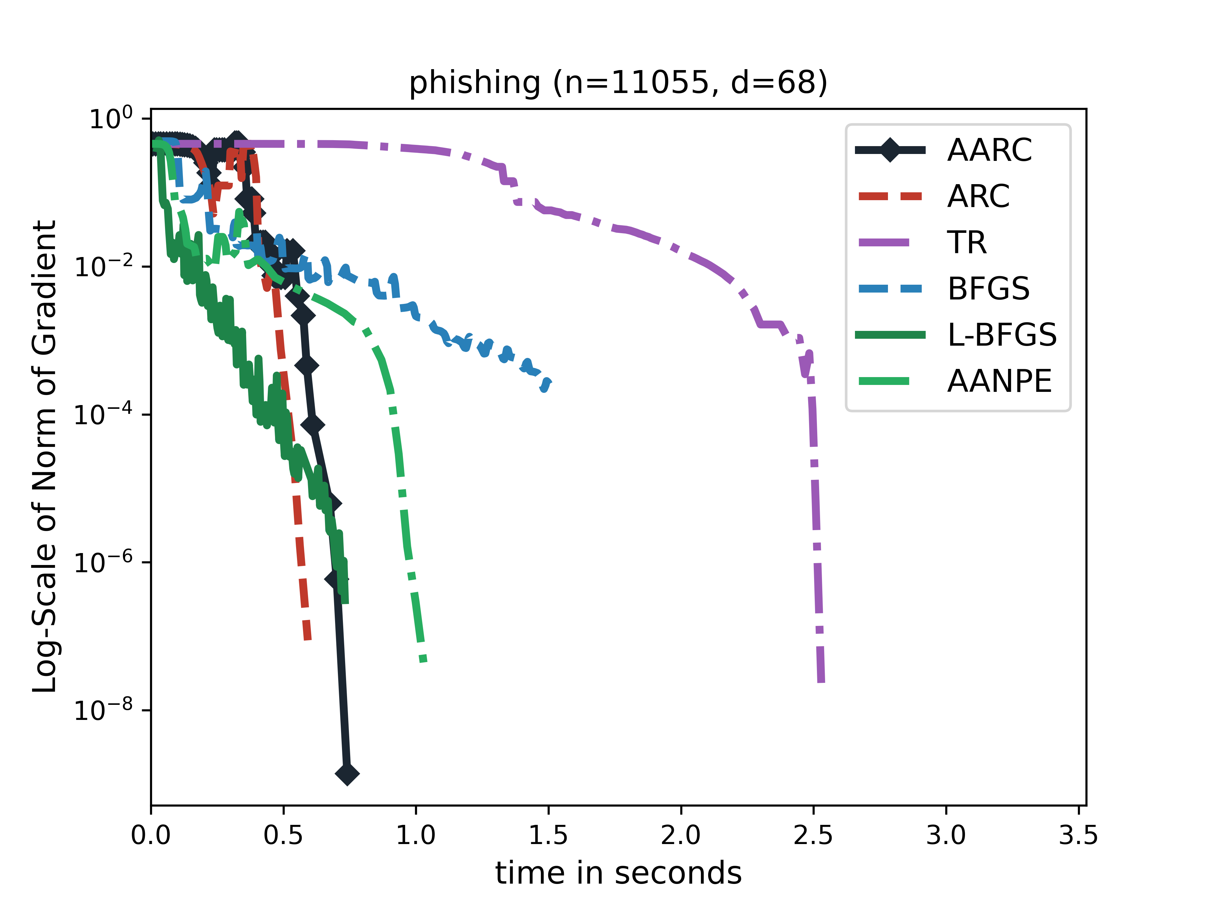
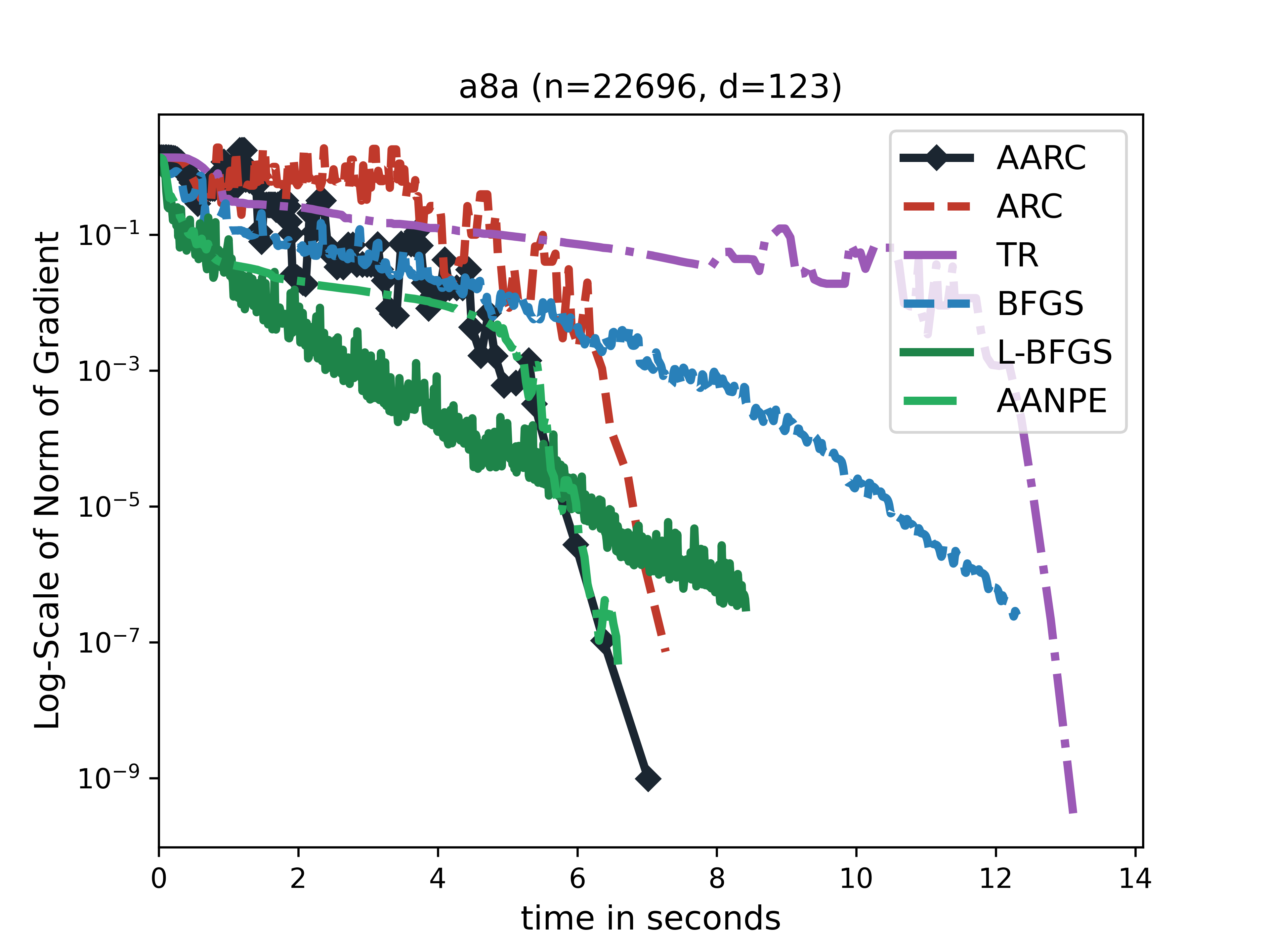
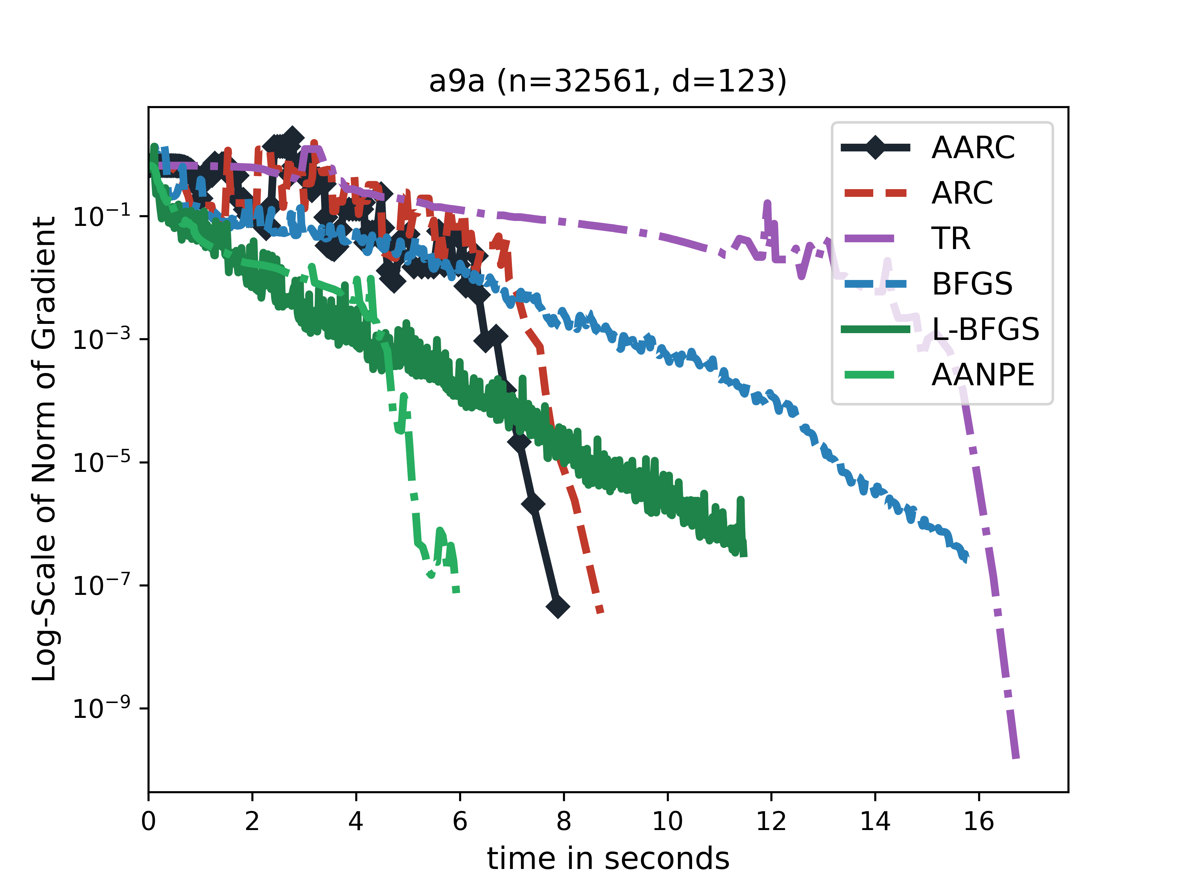
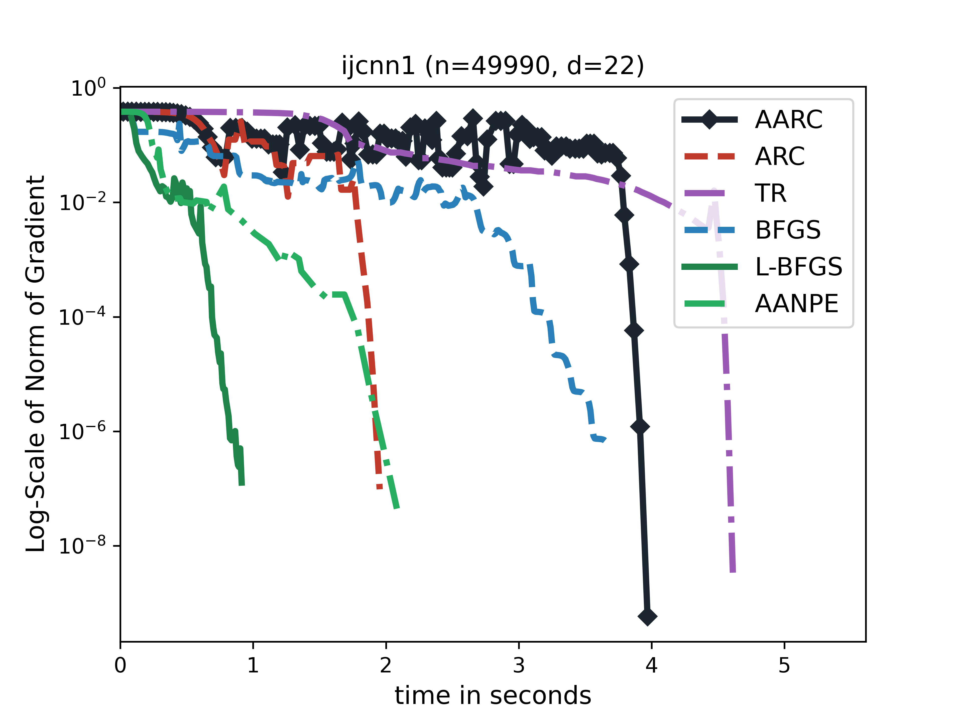
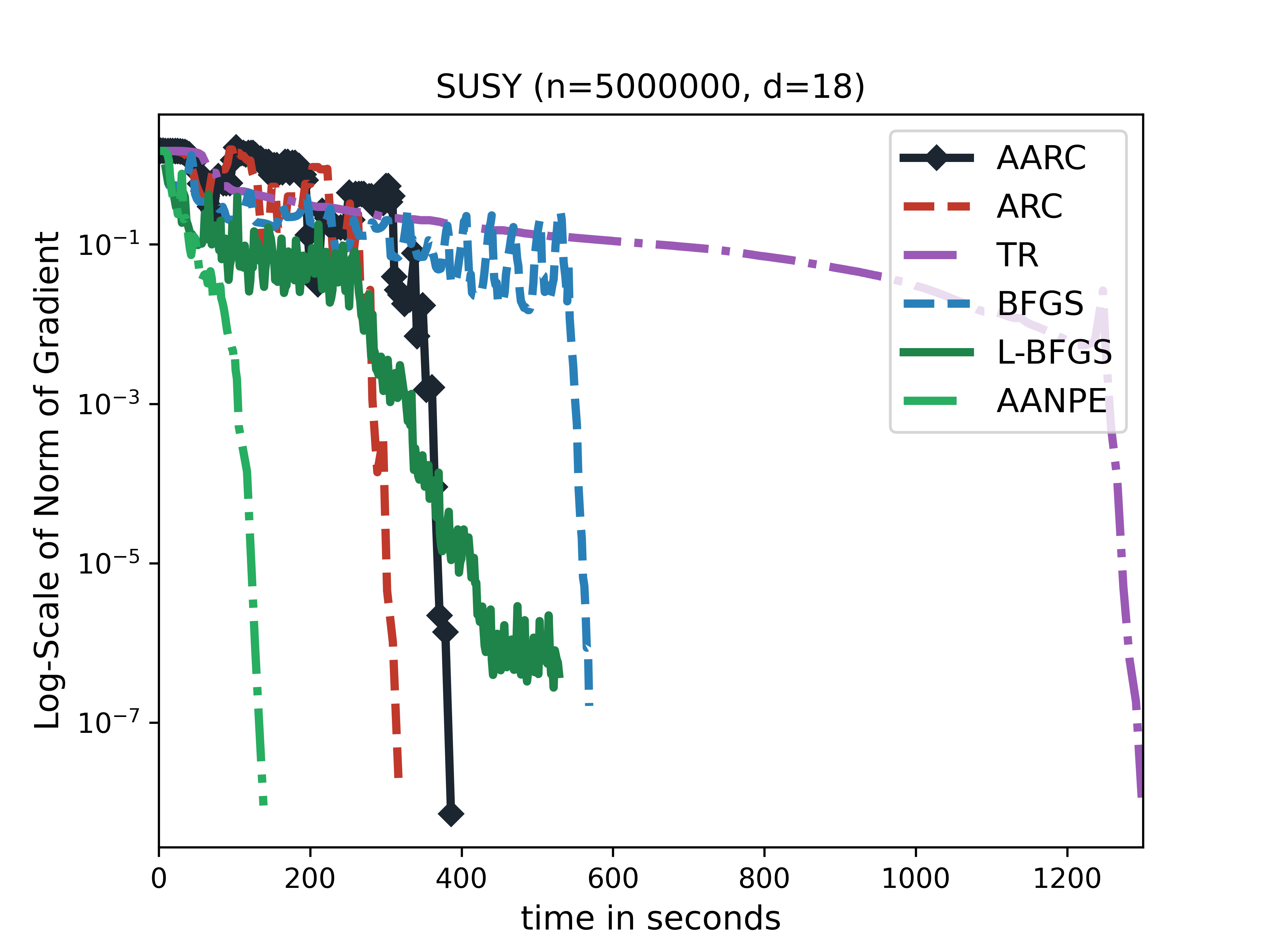
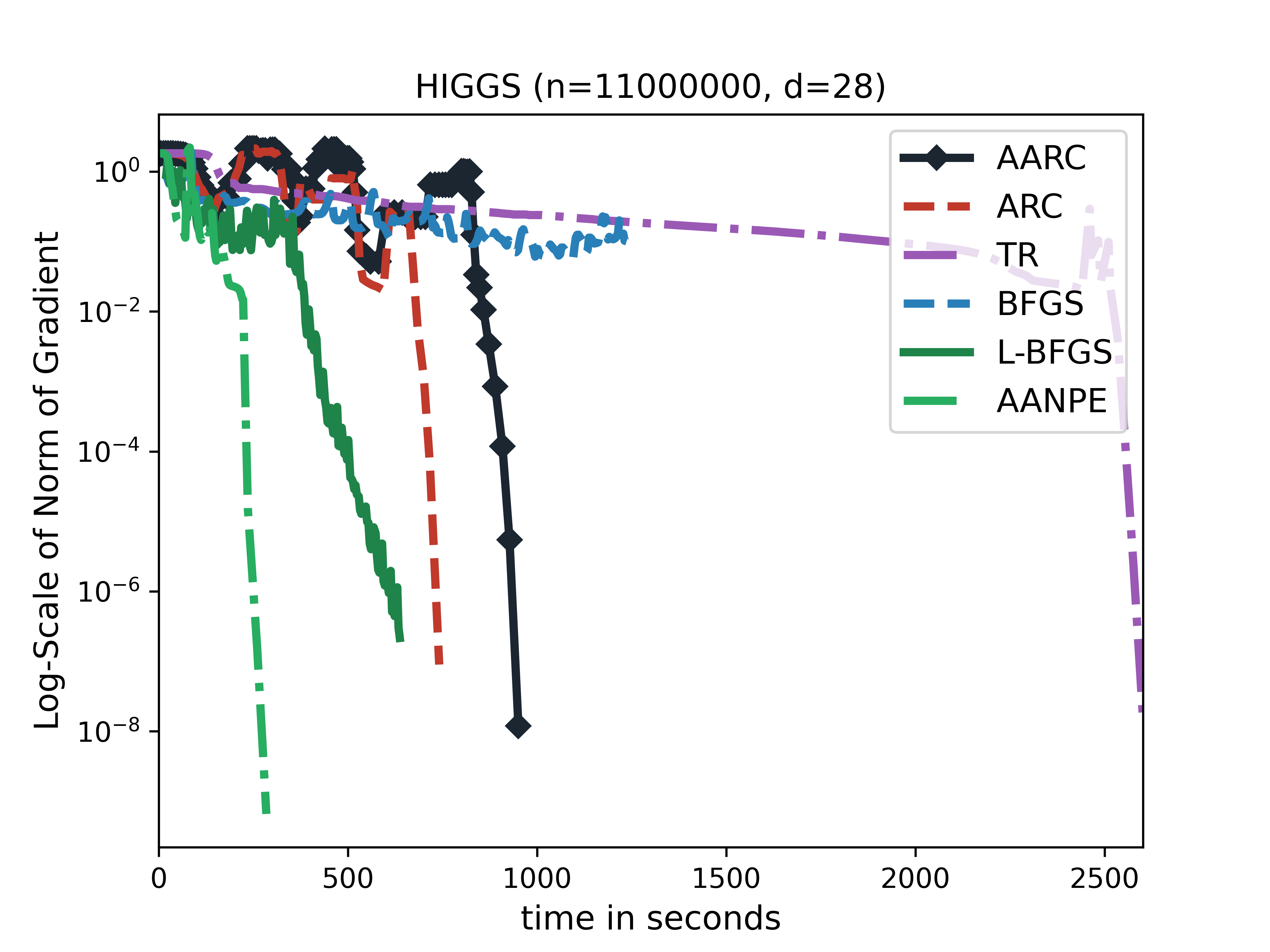
Figure 1: Log-scale norm of gradient v.s. time.

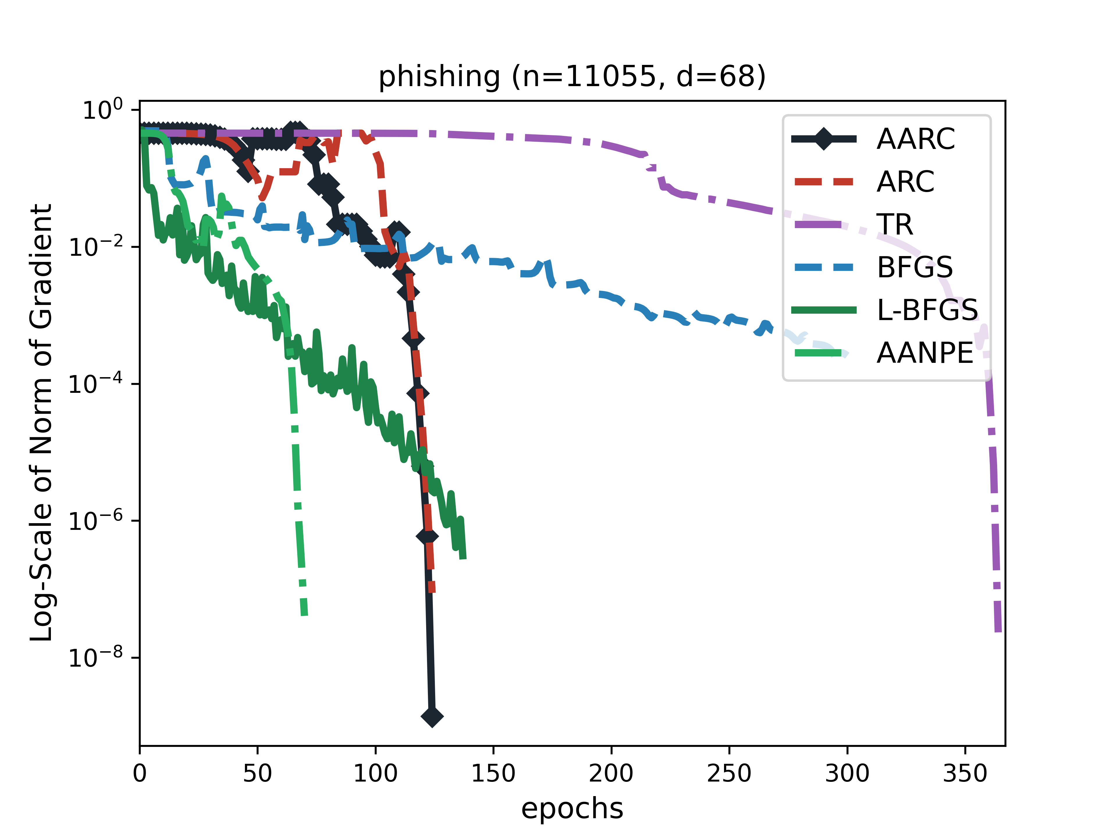
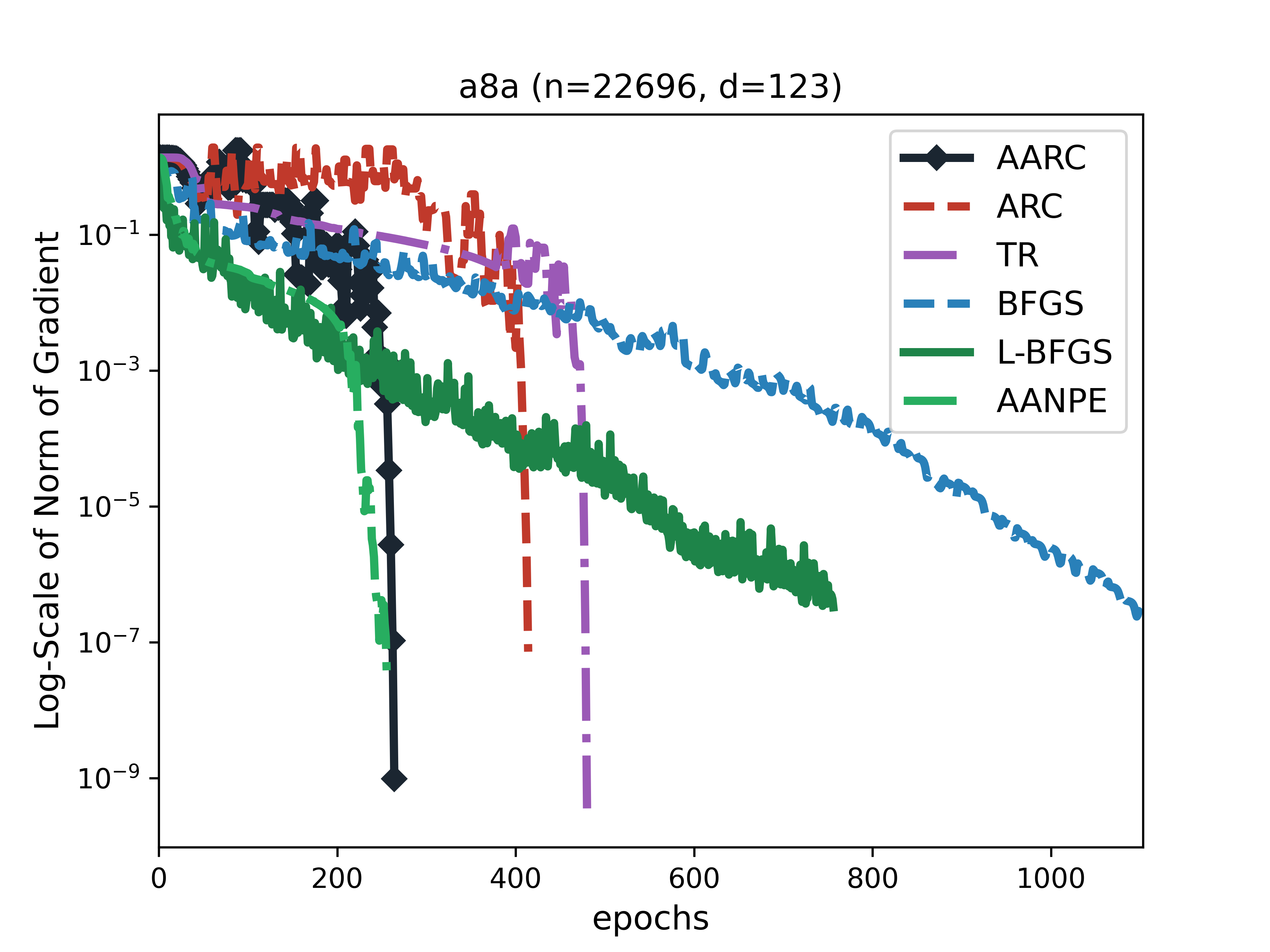
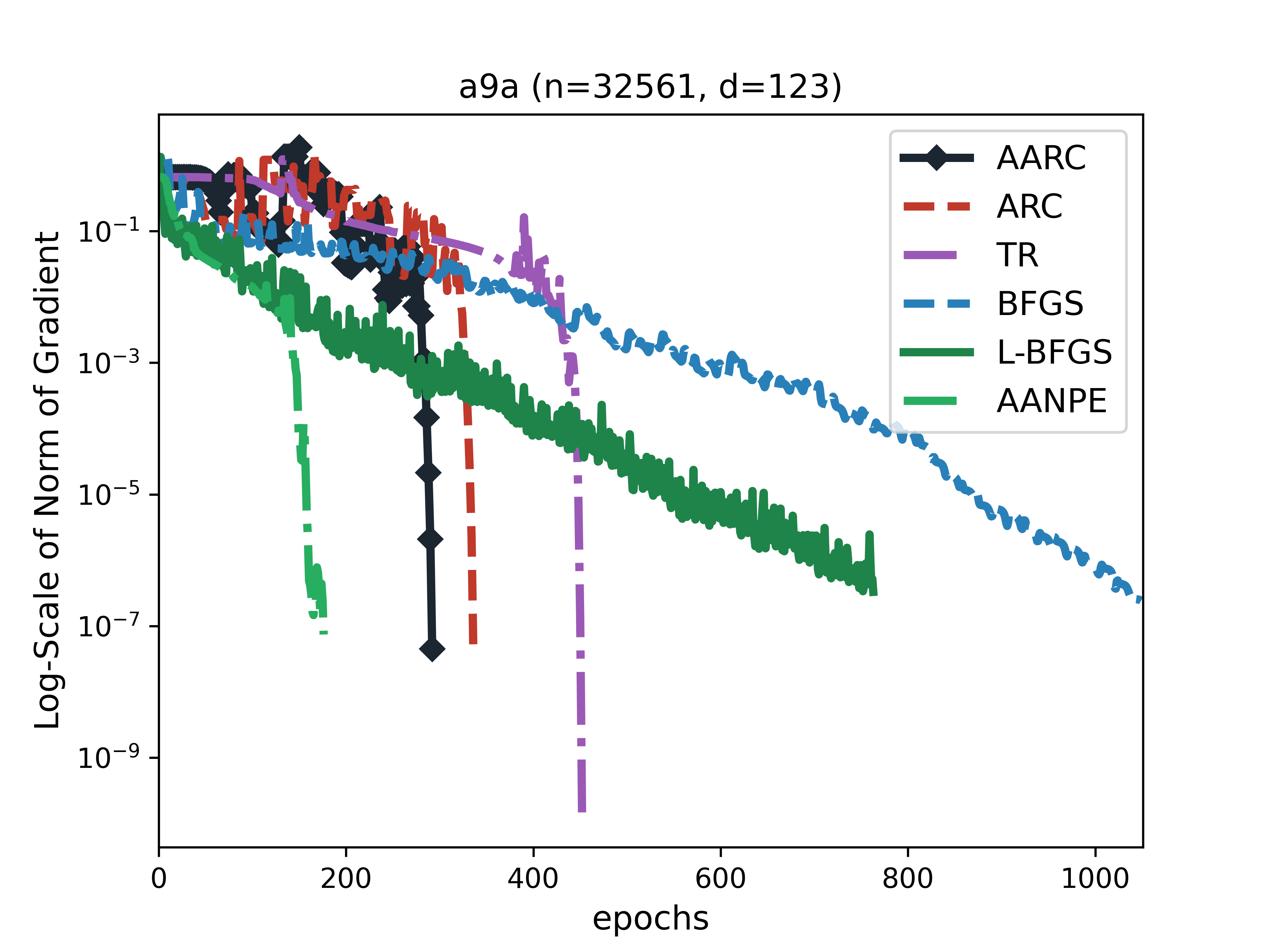
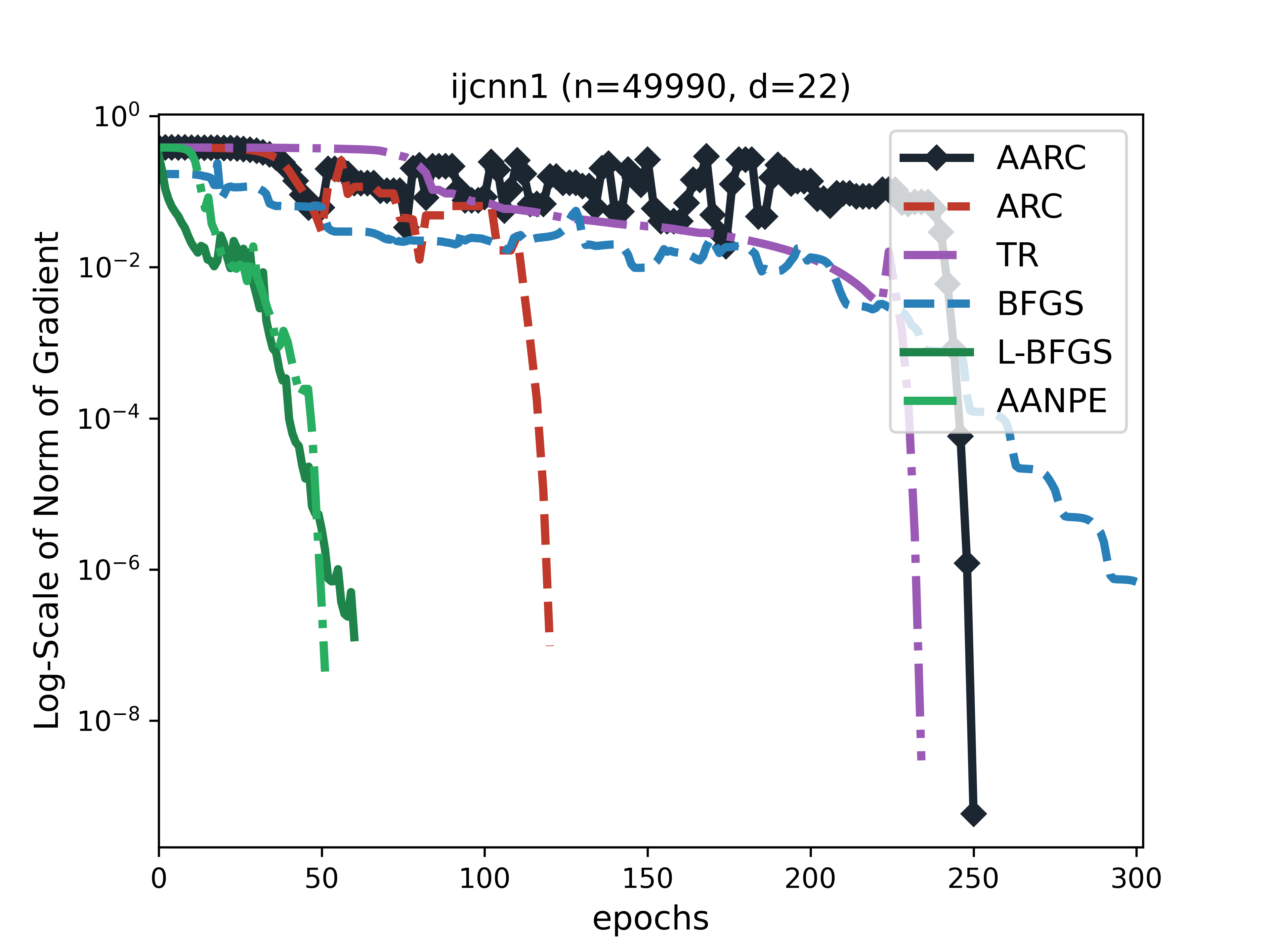
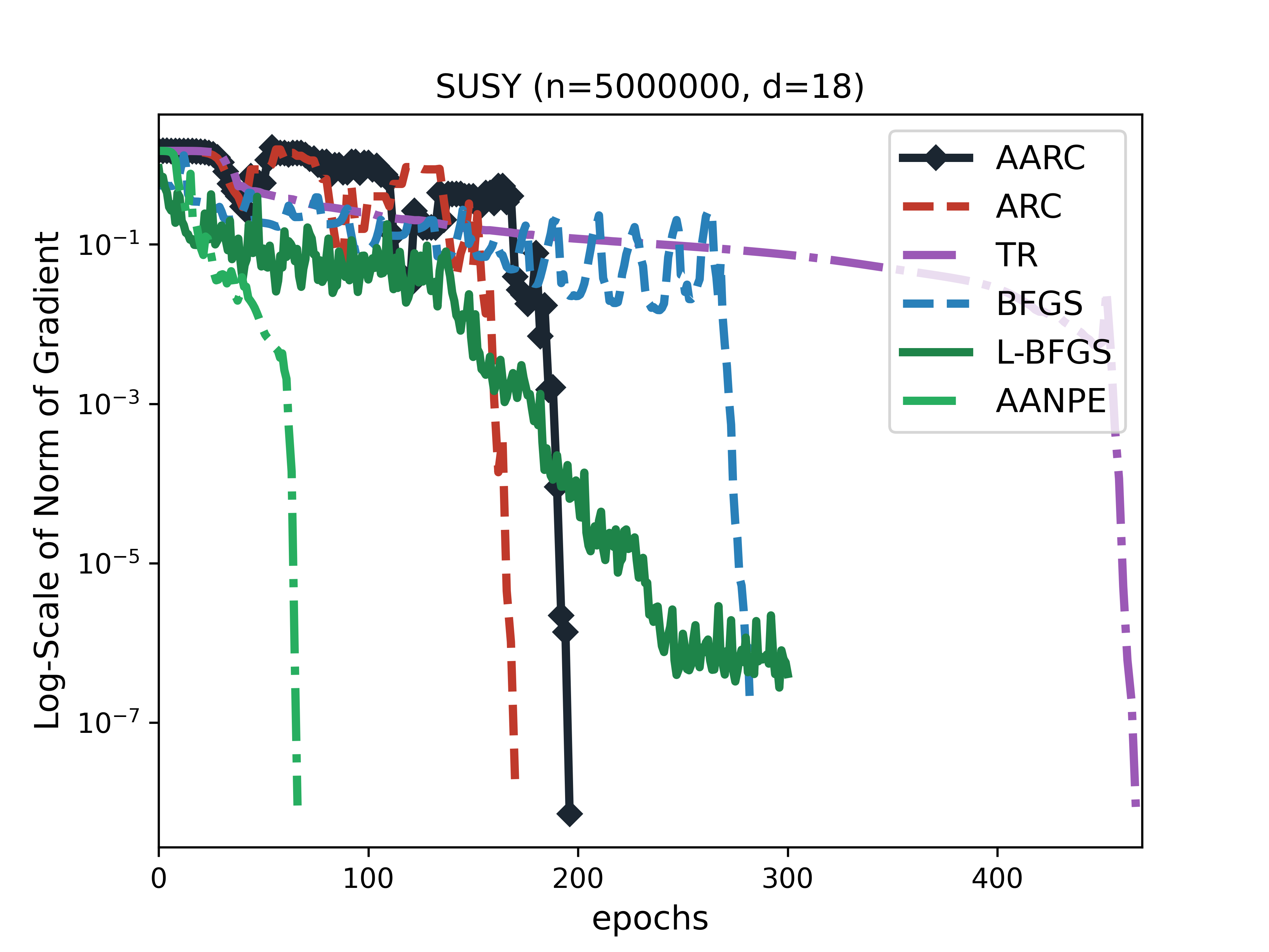
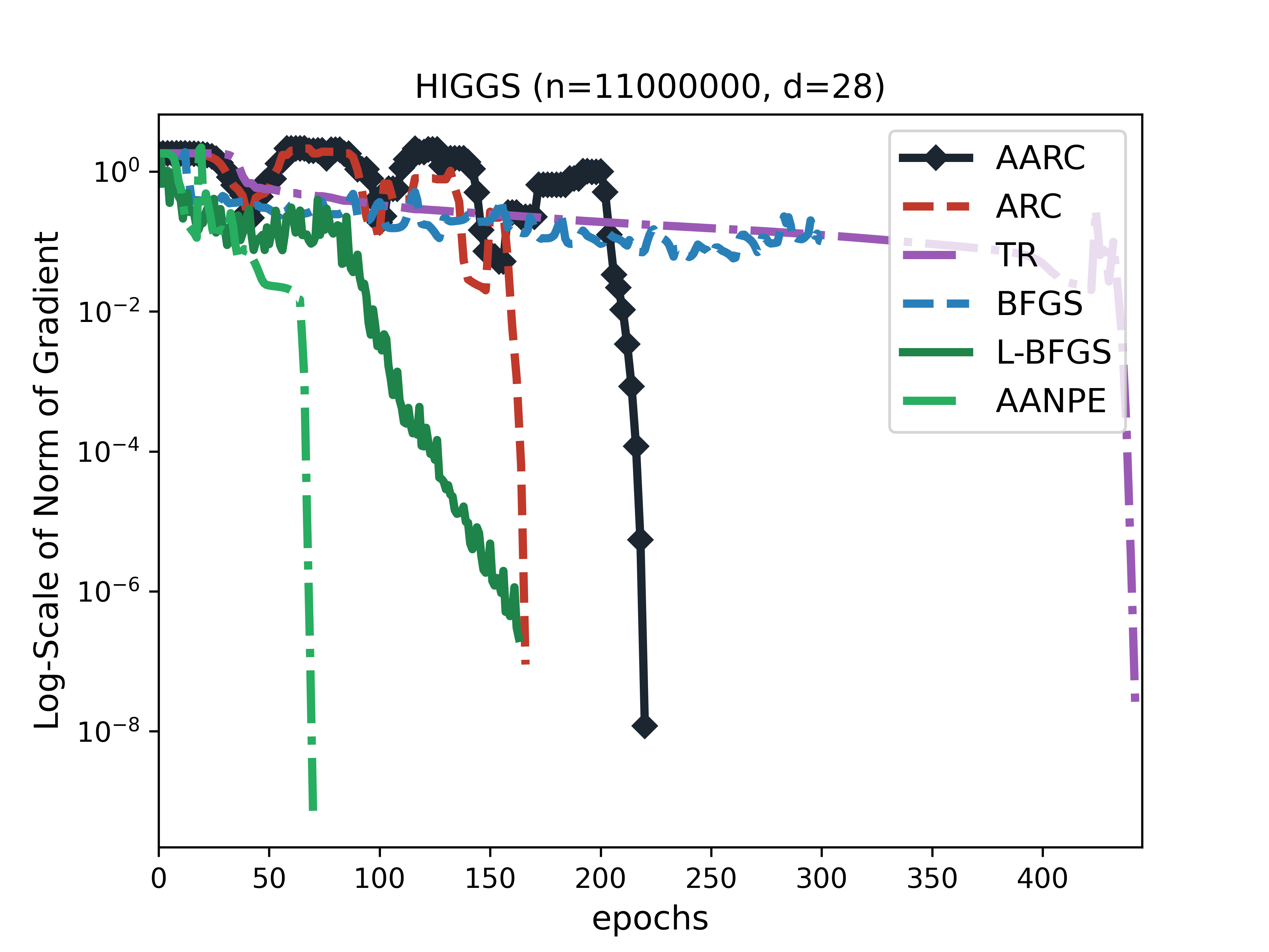
Figure 2: Log-scale norm of gradient v.s. No. epochs.

7.2 Comparison with Two Different Types of Sub-sampled Algorithms

In the second experiment, we compare our algorithm with two other sub-sampled second-order algorithms, one is the sub-sampled cubic regularized Newton method(SCR)[27], the other one is its accelerated variant, the sub-sampled accelerating adaptive cubic regularized Newton method(SACR)[14]. In the implementation, we set the initial point as zero vector and the number of the accelerated iterations as 5. Regarding the sampling scheme for the two other algorithms, we use the adaptive sampling scheme equipped with the default parameters in SCR as in their code. For SACR, We also follow their instruction in [14] on choosing the parameters.

We show the numerical results on the data sets in Figure 3, where the log-scaled norm of gradient v.s. the number of epochs is shown. We can see from the picture that the three algorithms have similar convergence behavior and the performance of our algorithm is comparable to that of other two sub-sampled second-order methods.

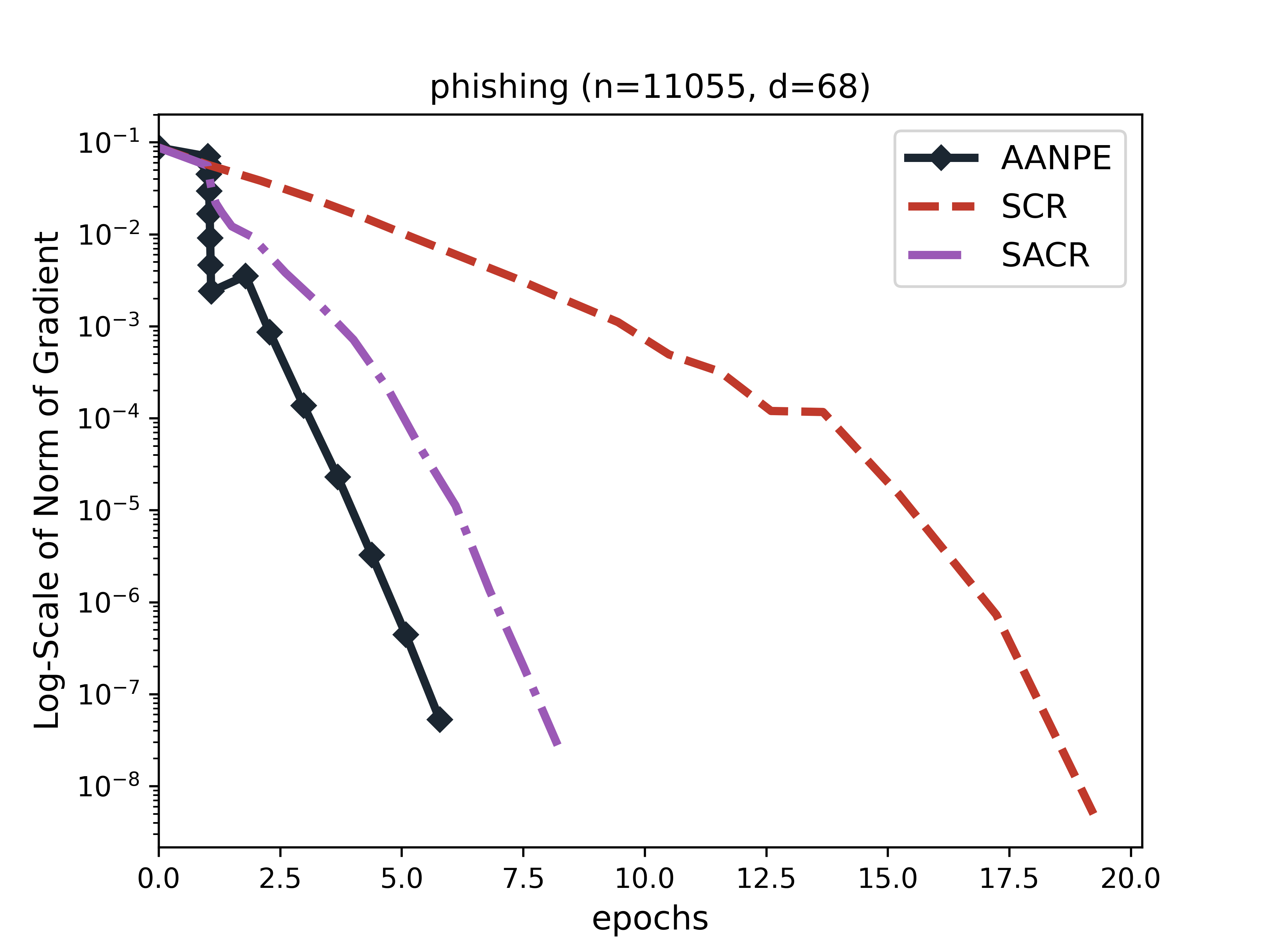
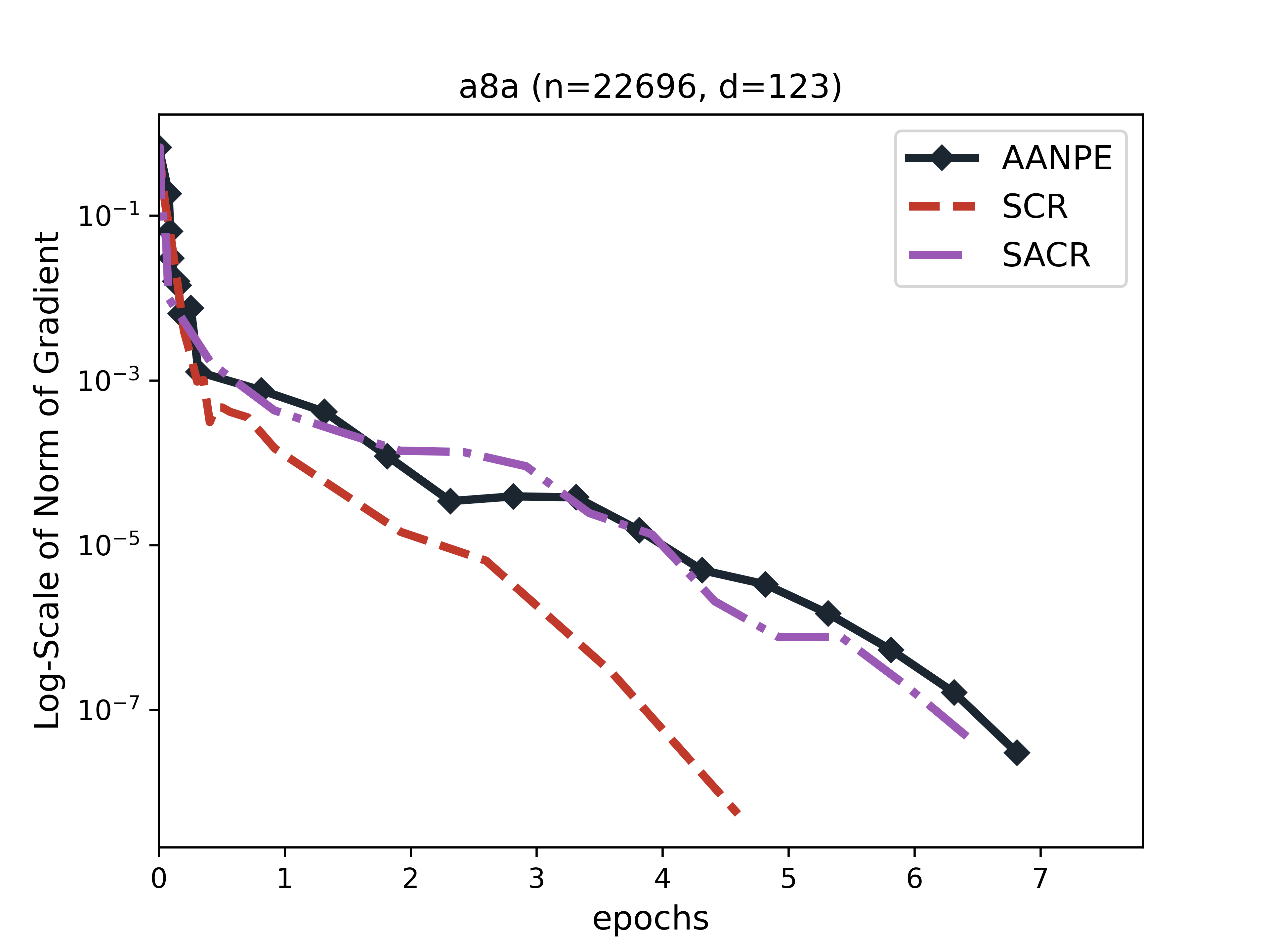
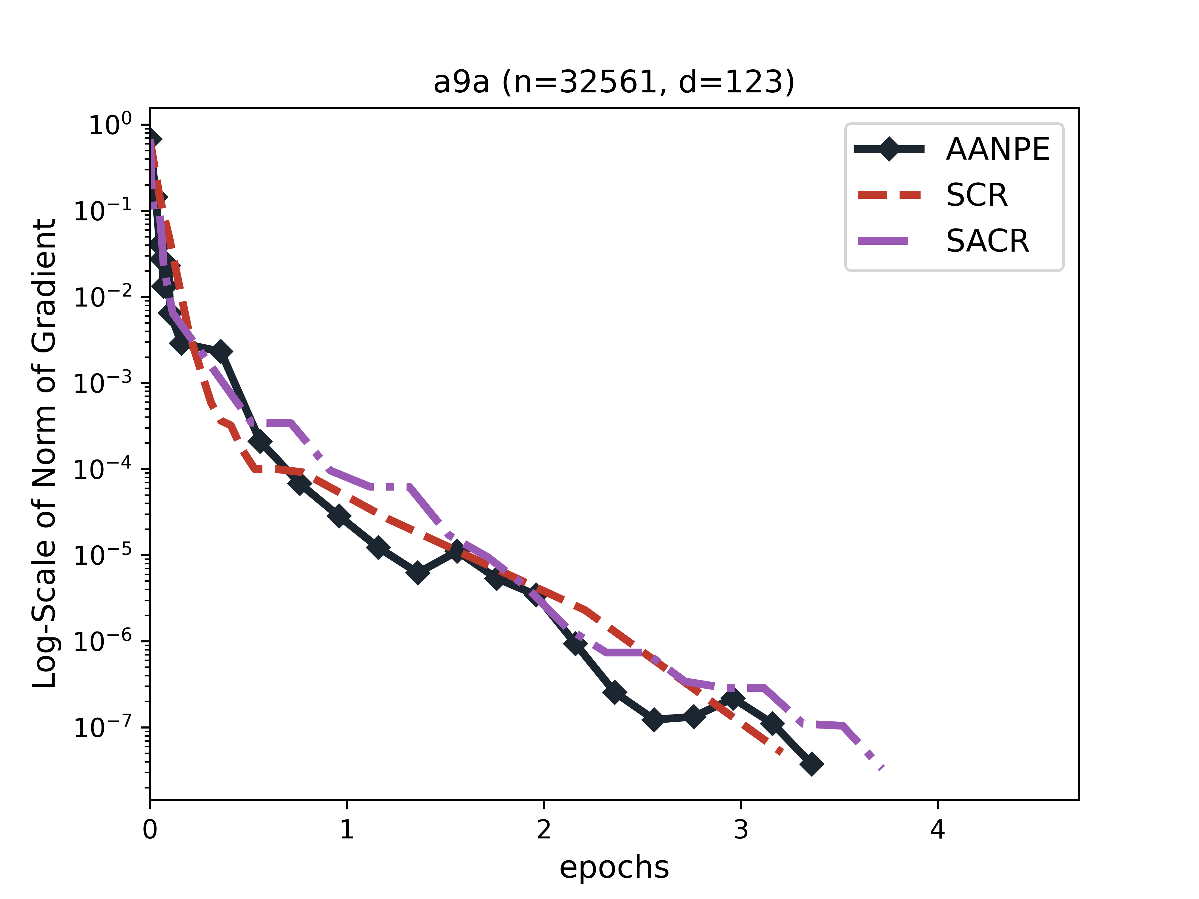
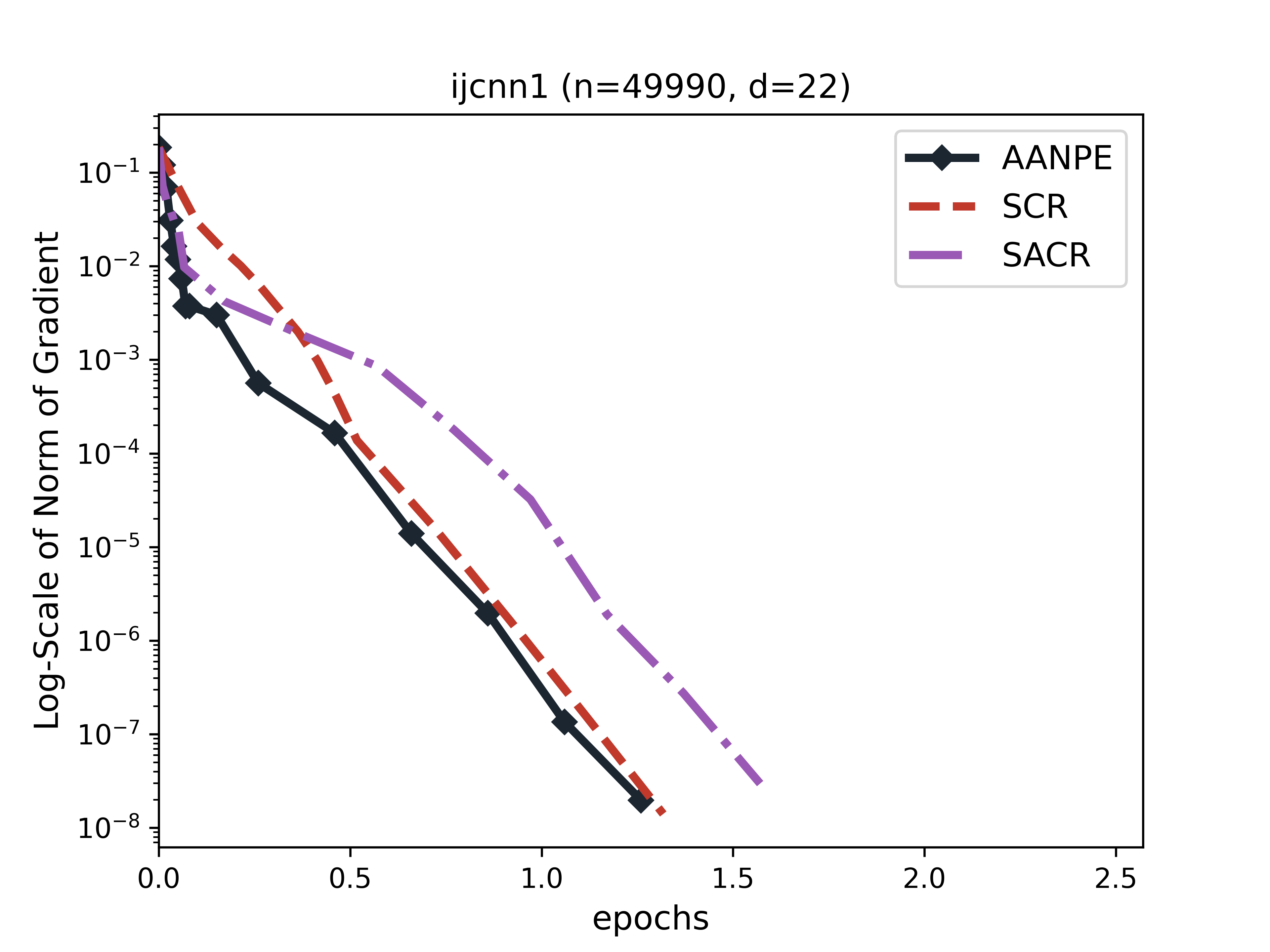
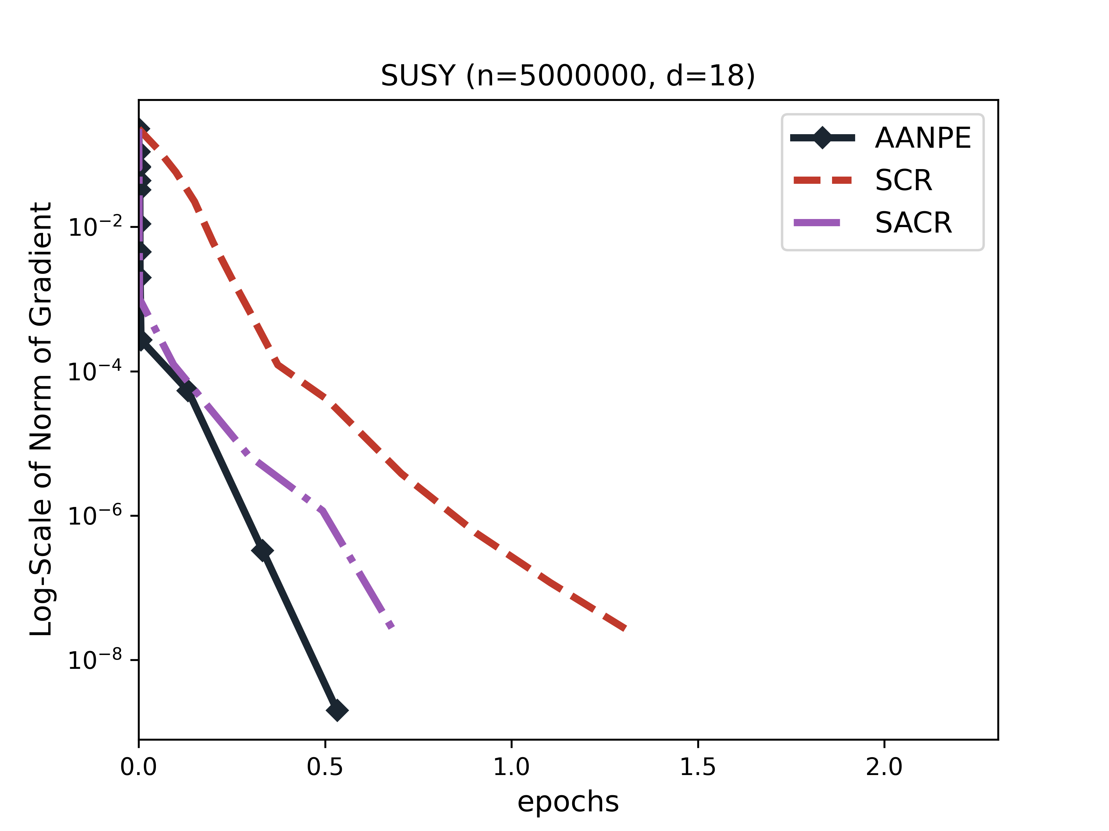
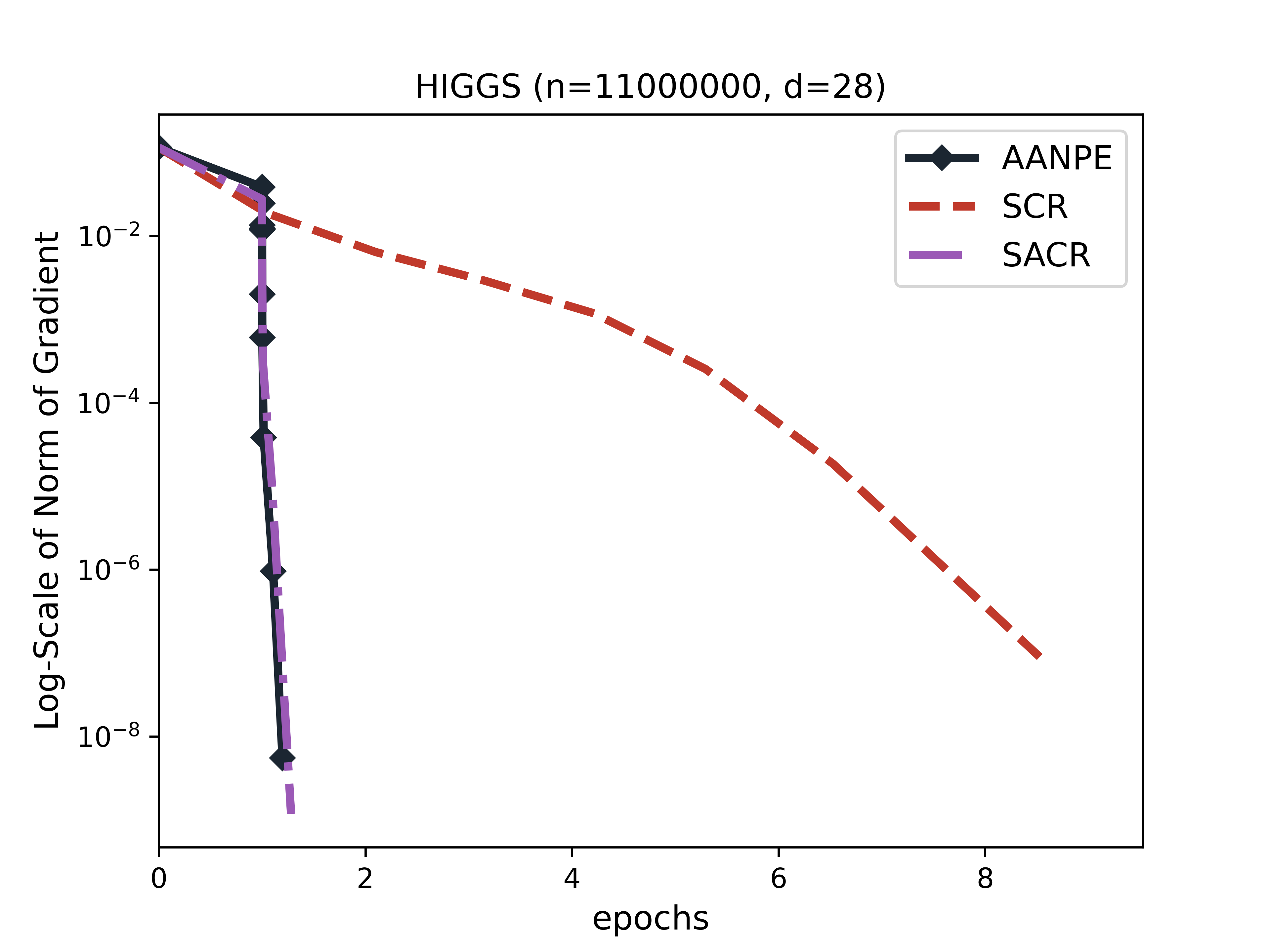
Figure 3: Log-scale norm of gradient v.s. No. epochs.

Appendix A Proof of Technical Lemmas

Proof to Proposition 3.1

Proof We first note that (3.20) and (3.21) can be derived by applying triangle inequality to (3.19). Thus it remains to prove (3.18) and (3.19).

From the definition, we can easily verify that (3.18) holds. As for (3.19), we can see that

$$\|u-v\| =\|\mathcal{G}(y)-\mathcal{G}_{x,\delta}(y)\|$$ (A.1)

$$=\|\mathcal{G}(y)-\mathcal{G}(x)-\mathcal{P}(x)(y-x)+\mathcal{G}^{\prime}(x)(y-x)-\mathcal{G}^{\prime}(x)(y-x)\|$$

$$\leq\|\mathcal{G}(y)-\mathcal{G}(x)-\mathcal{G}^{\prime}(x)(y-x)\|+\|\left(\mathcal{P}\left(x\right)-\mathcal{G}^{\prime}\left(x\right)\right)(y-x)\|$$

$$\leq\frac{L_{2}}{2}\|y-x\|^{2}+\delta\|y-x\|.$$

Where the last line can be derived by the Lipschitz continuity of $\mathcal{G}^{\prime}$, thus

$$\|\lambda v+y-x\|^{2}+2\lambda\epsilon =\|\lambda u+y-x+\lambda v-\lambda u\|^{2}+2\lambda\epsilon$$

$$\leq\left(\sqrt{\left\|\lambda u+y-x\right\|^{2}+2\lambda\epsilon}+\lambda\left\|u-x\right\|\right)^{2}$$

$$\leq\left(\hat{\sigma}\left\|y-x\right\|+\frac{L_{2}}{2}\left\|y-x\right\|^{2}+\delta\left\|y-x\right\|\right)^{2}$$

$$=\left(\hat{\sigma}+\frac{\lambda L_{2}}{2}\left\|y-x\right\|+\lambda\delta\right)\|y-x\|^{2}.$$

The second line can be verified by expanding the squared term on the right-hand side, the third line is from Definition 3.5, and the last line is from (A.1). ∎

Proof to Proposition 4.4

Proof For simplicity, let $y=y_{\mathcal{B}}(\lambda;x)$ and $\tilde{y}=y_{\tilde{\mathcal{B}}}(\lambda;\tilde{x})$, then there exist $v\in\mathcal{B}(y)$ and $\tilde{v}\in\tilde{\mathcal{B}}(\tilde{y})$ such that

$$\lambda v+y-x=0,\ \lambda\tilde{v}+\tilde{y}-\tilde{x}=0.$$ (A.2)

As a consequence,

$$\varphi_{\mathcal{B}}(\lambda;x)=\lambda^{2}\|v\|,\ \varphi_{\tilde{\mathcal{B}}}(\lambda;\tilde{x})=\lambda^{2}\|\tilde{v}\|.$$

Let $u:=v+\mathcal{G}_{\tilde{x},\delta}(y)-\mathcal{G}_{x,\delta}(y),$ note the that $v\in\mathcal{B}(y)$, then we know

$$u\in\mathcal{B}(y)+\mathcal{G}_{\tilde{x},\delta}(y)-\mathcal{G}_{x,\delta}(y)=\mathcal{T}_{x,\delta}(y)+\mathcal{G}_{\tilde{x},\delta}(y)-\mathcal{G}_{x,\delta}(y)=\mathcal{G}_{\tilde{x},\delta}(y)+\mathcal{H}(y)=\tilde{\mathcal{B}}(y)$$

and

$$\lambda u+y-\tilde{x}=\lambda v+y-x+(\tilde{x}-x)+\lambda(u-v)=(\tilde{x}-x)+\lambda(u-v).$$ (A.3)

Combine (A.3) with (A.2) we conclude that

$$\lambda(u-\tilde{v})+(y-\tilde{y})=(\tilde{x}-x)+\lambda(u-v).$$ (A.4)

Since $u\in\tilde{\mathcal{B}}(y)$ and $\tilde{v}\in\tilde{\mathcal{B}}(\tilde{y})$, it follows from the monotonicity of $\tilde{\mathcal{B}}$ that $\langle u-\tilde{v},y-\tilde{y}\rangle\geq 0$, which together with (A.4) and the triangle inequality for norms implies that

$$\lambda\|u-\tilde{v}\|\leq\|\tilde{x}-x\|+\lambda\|u-v\|$$

and hence that

$$\lambda\|v-\tilde{v}\|\leq\|\tilde{x}-x\|+2\lambda\|u-v\|.$$

This implies

$$|\varphi_{\mathcal{B}}(\lambda;x)-\varphi_{\tilde{\mathcal{B}}}(\lambda;\tilde{x})|=\lambda^{2}\left|\left\|v\right\|-\left\|\tilde{v}\right\|\right|\leq\lambda^{2}\left\|v-\tilde{v}\right\|\leq\lambda\left(\left\|\tilde{x}-x\right\|+2\lambda\left\|u-v\right\|\right).$$

Now, use the definition of $u$, we have

$$u-v =\mathcal{G}_{\tilde{x},\delta}(y)-\mathcal{G}_{x,\delta}(y)=\mathcal{G}(\tilde{x})+\mathcal{P}(\tilde{x})(y-\tilde{x})-\left(\mathcal{G}(x)+\mathcal{P}(x)(y-x)\right)$$

$$=\mathcal{G}(\tilde{x})+\mathcal{P}(\tilde{x})(x-\tilde{x})-\mathcal{G}(x)+\left(\mathcal{P}(\tilde{x})-\mathcal{P}(x)\right)(y-x)$$

and hence

$$\lambda\|u-v\| \leq\lambda\|\mathcal{G}(\tilde{x})+\mathcal{P}(\tilde{x})(x-\tilde{x})-\mathcal{G}(x)\|+\lambda\|\mathcal{P}(\tilde{x})-\mathcal{P}(x)\|\|y-x\|$$

$$\leq\lambda\|\mathcal{G}(\tilde{x})+\mathcal{G}^{\prime}(\tilde{x})(x-\tilde{x})-\mathcal{G}(x)\|+\lambda\|\mathcal{P}(\tilde{x})-\mathcal{G}^{\prime}(\tilde{x})|\|x-\tilde{x}\|+\lambda\|\mathcal{P}(\tilde{x})-\mathcal{P}(x)\|\|y-x\|$$

$$\leq\frac{\lambda L_{2}}{2}\|\tilde{x}-x\|^{2}+\lambda\delta\|\tilde{x}-x\|+\lambda L_{2}\|\tilde{x}-x\|\|y-x\|$$

$$\leq\frac{\lambda L_{2}}{2}\|\tilde{x}-x\|^{2}+\lambda\delta\|\tilde{x}-x\|+\lambda L_{2}\|\tilde{x}-x\|\|y-x\|$$

$$=\frac{\lambda L_{2}}{2}\|\tilde{x}-x\|^{2}+\lambda\delta\|\tilde{x}-x\|+L_{2}\|\tilde{x}-x\|\varphi_{\mathcal{B}}(\lambda;x)$$

$$\leq\frac{\lambda L_{2}}{2}\|\tilde{x}-x\|^{2}+C\|\tilde{x}-x\|+L_{2}\|\tilde{x}-x\|\varphi_{\mathcal{B}}(\lambda;x)$$

Now we can conclude that

$$|\varphi_{\mathcal{B}}(\lambda;x)-\varphi_{\tilde{\mathcal{B}}}(\lambda;\tilde{x})|\leq(1+2C)\lambda\|\tilde{x}-x\|+L_{2}\lambda^{2}\|\tilde{x}-x\|^{2}+2L_{2}\lambda\|\tilde{x}-x\|\varphi_{\mathcal{B}}(\lambda;x).$$

This inequality and the symmetric one obtained by interchanging $x$ and $\tilde{x}$ in the latter relation then imply (4.4). ∎

Proof to Proposition 4.5

Proof Suppose $\lambda\geq\max\left\{\sqrt{\frac{\alpha}{\bar{v}}\left(1+\hat{\sigma}+C+\frac{L_{2}\alpha}{2}\right)},\left(\frac{\hat{\sigma}^{2}\alpha^{2}}{2\bar{\epsilon}}\right)^{\frac{1}{3}}\right\}$ and $\lambda\|y-x\|\leq\alpha$. From proposition 3.1 we know that

$$\|v\|\leq\frac{1}{\lambda}\left(1+\hat{\sigma}+C+\frac{L_{2}\lambda}{2}\|y-x\|\right)\|y-x\|\leq\left(1+\hat{\sigma}+C+\frac{L_{2}\alpha}{2}\right)\frac{\alpha}{\lambda^{2}}\leq\bar{v}$$

and

$$\epsilon\leq\frac{\hat{\sigma}^{2}}{2\lambda}\|y-x\|^{2}\leq\frac{\hat{\sigma}^{2}\alpha^{2}}{2\lambda^{3}}\leq\bar{\epsilon}.$$

This contradicts (3.11). ∎

Proof to Proposition 4.6

Proof First, we note that (4.10) follows immediately from (4.8) and (4.9). Let $\mathcal{B}_{-}:=\mathcal{T}_{x_{-}^{0},\delta}$ and $\mathcal{B}_{+}:=\mathcal{T}_{x_{+}^{0},\delta}$. Since a $(\hat{\sigma},\delta)$-approximate Newton solution at $(\lambda_{-}^{0},x_{-}^{0})$ is a $\hat{\sigma}$-approximate solution with $\mathcal{B}=\mathcal{B}_{-}$, it follows from Proposition 4.2 with $\mathcal{B}=\mathcal{B}_{-}$ that

$$\lambda_{-}^{0}\|y_{-}^{0}-x_{-}^{0}\|\leq\frac{\varphi_{\mathcal{B}_{-}}(\lambda_{-}^{0};x_{-}^{0})}{1-\hat{\sigma}}\leq\frac{\lambda_{-}^{0}\varphi_{\mathcal{B}_{-}}(\lambda_{+}^{0};x_{-}^{0})}{(1-\hat{\sigma})\lambda_{+}^{0}},$$

where the last inequality is due to (4.10) and Proposition 4.1(b) with $\mathcal{B}=\mathcal{B}_{-},\tilde{\lambda}=\lambda_{-}^{0}$, and $\lambda=\lambda_{+}^{0}$. Also Proposition 4.4 with $\lambda=\lambda_{+}^{0},x=x_{-}^{0}$, and $\tilde{x}=x_{+}^{0}$ and the definition of $\theta_{+}^{0}$ implies that

$$\varphi_{\mathcal{B}_{-}}(\lambda_{+}^{0};x_{-}^{0}) \leq(2L_{2}\theta_{+}^{0}+1)\varphi_{\mathcal{B}_{+}}(\lambda_{+}^{0};x_{+}^{0})+(1+2C)\theta_{+}^{0}+L_{2}(\theta_{+}^{0})^{2}$$

$$\leq(2L_{2}\theta_{+}^{0}+1)(1+\hat{\sigma})\lambda_{+}^{0}\|y_{+}^{0}-x_{+}^{0}\|+(1+2C)\theta_{+}^{0}+L_{2}(\theta_{+}^{0})^{2}$$

$$\leq\frac{\alpha(1-\hat{\sigma})\lambda_{+}^{0}}{\lambda_{-}^{0}},$$

where the last inequality follows from the definition of $\lambda_{-}^{0}$. Combining the above two inequalities, we then conclude that (4.11) holds. ∎

Proof to Corollary 4.1

Proof From (4.7) and Proposition 4.5 we can easily know that the first claim holds. From (4.13) we know

$$\lambda_{-}^{0}\leq\frac{\alpha_{-}(1-\hat{\sigma})\lambda_{+}^{0}}{(1+\hat{\sigma})(1+2L_{2}\theta_{+}^{0})\lambda_{+}^{0}\|y_{+}^{0}-x_{+}^{0}\|+(1+2C)\theta_{+}^{0}+L_{2}(\theta_{+}^{0})^{2}},$$

so in the view of Proposition 4.6 we have

$$\lambda_{-}^{0}\|y_{-}^{0}-x_{-}^{0}\|\leq\alpha_{-}.$$

∎

Proof to Lemma 5.1

Proof Note that as in Proposition 4.5, when $\lambda_{k+1}\geq\Lambda\left(\frac{2\sigma_{l}}{L_{2}}\right)$, the while loop will terminate. When the length of the while loop approaches $\log_{\gamma}\frac{\delta_{\max}\Lambda\left(\frac{2\sigma_{l}}{L_{2}}\right)}{C}$, we have $\lambda_{k+1}=\frac{C}{\delta_{k}}\geq\Lambda\left(\frac{2\sigma_{l}}{L_{2}}\right)$. ∎

Proof to Proposition 4.7

Proof Let $\mathcal{B}$ denote the exact first-order approximate of $\mathcal{T}$ at $x$, then from Monteiro and Svaiter [36, Theorem 7.11] we know that:

$$\varphi_{\mathcal{B}}(\lambda;x)\leq\lambda\|x-x_{*}\|+\lambda^{2}L_{2}\|x-x_{*}\|^{2}.$$ (A.5)

Since

$$\varphi_{\mathcal{B}}(\lambda;x)=\lambda\|x-(I+\lambda\mathcal{B})^{-1}(x)\|,$$

$$\varphi_{\mathcal{T}_{x,\delta}}(\lambda;x)=\lambda\|x-(I+\lambda\mathcal{T}_{x,\delta})^{-1}(x)\|.$$

So we let $y_{1}=(I+\lambda\mathcal{B})^{-1}(x)$ and $y_{2}=(I+\lambda\mathcal{T}_{x,\delta})^{-1}(x)$, then we have

$$\varphi_{\mathcal{B}}(\lambda;x) =\lambda\|x-y_{1}\|,$$ (A.6)

$$\varphi_{\mathcal{T}_{x,\delta}}(\lambda;x) =\lambda\|x-y_{2}\|,$$ (A.7)

and

$$y_{1}+\lambda u=x,\ u=\mathcal{G}_{x}(y)+u_{h},\ u_{h}\in\mathcal{H}(y_{1}),$$ (A.8)

$$y_{2}+\lambda v=x,\ v=\mathcal{G}_{x,\delta}(y)+v_{h},\ v_{h}\in\mathcal{H}(y_{2}).$$ (A.9)

$\mathcal{G}_{x}(y):=\mathcal{G}(x)+\mathcal{G}^{\prime}(x)(y-x)$. Subtracting the equations (A.8) and (A.9),

$$0 =y_{1}-y_{2}+\lambda(u-v)$$

$$=y_{1}-y_{2}+\lambda\mathcal{G}^{\prime}(x)(y_{1}-x)+\lambda u_{h}-\lambda\mathcal{P}(x)(y_{2}-x)-\lambda v_{h}$$

$$=(y_{1}-y_{2})+\lambda\mathcal{G}^{\prime}(x)y_{1}-\lambda\mathcal{P}(x)y_{2}+\lambda(\mathcal{P}(x)-\mathcal{G}^{\prime}(x))x+\lambda(u_{h}-v_{h})$$

$$=(y_{1}-y_{2})+\lambda\mathcal{G}^{\prime}(x)(y_{1}-y_{2})-\lambda(\mathcal{P}(x)-\mathcal{G}^{\prime}(x))y_{2}+\lambda(\mathcal{P}(x)-\mathcal{G}^{\prime}(x))x+\lambda(u_{h}-v_{h}).$$

Then we know

$$(1+\lambda\mathcal{G}^{\prime}(x))(y_{1}-y_{2})=(\mathcal{P}(x)-\mathcal{G}^{\prime}(x))\lambda(y_{2}-x)-\lambda(u_{h}-v_{h}).$$

Note that $\mathcal{G}$ is monotone and differentiable, as a consequence,

$$\|y_{1}-y_{2}\| \leq\lambda\|\mathcal{P}(x)-\mathcal{G}^{\prime}(x)\|\|y_{2}-x\|+\lambda\|u_{h}-v_{h}\|$$ (A.10)

$$\leq\delta\lambda\|y_{2}-x\|+2L^{\prime}\lambda$$

$$=\delta\varphi_{\mathcal{T}_{x}}(\lambda;x)+2L^{\prime}\lambda,$$

the first inequality is from that $\mathcal{G}$ is maximal monotone, the second inequality comes from the boundedness of $\mathcal{H}$. From the above inequation, (A.7) and (A.5) we know

$$\|x-(I+\lambda\mathcal{T}_{x})^{-1}(x)\| =\|x-y_{2}\|$$ (A.11)

$$\leq\|x-y_{1}\|+\|y_{1}-y_{2}\|$$

$$\leq\delta\varphi_{\mathcal{T}_{x}}(\lambda;x)+2L^{\prime}\lambda+\|x-x_{*}\|+\lambda L_{2}\|x-x_{*}\|^{2},$$

note that $\lambda\delta\leq C$, (A.11) implies

$$\varphi_{\mathcal{T}_{x}}(\lambda;x)\leq C\varphi_{\mathcal{T}_{x}}(\lambda;x)+2L^{\prime}\lambda^{2}+\lambda\|x-x_{*}\|+\lambda^{2}L_{2}\|x-x_{*}\|^{2}.$$ (A.12)

Then the proof is finished. ∎

Proof to Lemma 5.4

Proof For any $v\in\partial_{\epsilon}h(x)$, let $y_{\alpha}=x+\alpha v$, from (2.4), we have

$$\alpha\|v\|^{2} =\langle y-x,v\rangle$$

$$\leq h(y)-h(x)+\epsilon$$

$$\leq L^{\prime}\|y-x\|+\epsilon$$

$$=\alpha L^{\prime}\|v\|+\epsilon.$$

The second last line comes from the Lipschitz continuity of $h$. Let $\alpha\to+\infty$ we have $\|v\|\leq L^{\prime}$. ∎

Proof to Lemma 6.1

Proof Since sample size

$$\left|\mathcal{S}\right|\geq\frac{16L_{1}^{2}}{\kappa^{2}}\log\left(\frac{2Nd}{\delta^{\prime}}\right),$$

as in [48], for each $i=1,2,\dotsb,N$ we have

$$\textnormal{Prob}\left(\left\|\tilde{H}(x_{i})-\nabla^{2}g(x_{i})\right\|\geq\kappa\right)<\frac{\delta^{\prime}}{N}.$$

Then the corollary is from the subadditivity of the probability. ∎

References

• Agafonov etย al. [2023a] Artem Agafonov, Dmitry Kamzolov, Pavel Dvurechensky, Alexander Gasnikov, and Martin Takรกฤ. Inexact tensor methods and their application to stochastic convex optimization. Optimization Methods and Software, pages 1โ€“42, 2023a.
• Agafonov etย al. [2023b] Artem Agafonov, Dmitry Kamzolov, Alexander Gasnikov, Kimon Antonakopoulos, Volkan Cevher, and Martin Takรกฤ. Advancing the lower bounds: An accelerated, stochastic, second-order method with optimal adaptation to inexactness. arXiv preprint arXiv:2309.01570, 2023b.
• Agarwal etย al. [2017] Naman Agarwal, Brian Bullins, and Elad Hazan. Second-order stochastic optimization for machine learning in linear time. The Journal of Machine Learning Research, 18(1):4148โ€“4187, 2017.
• Antonakopoulos etย al. [2022] Kimon Antonakopoulos, Ali Kavis, and Volkan Cevher. Extra-newton: A first approach to noise-adaptive accelerated second-order methods. Advances in Neural Information Processing Systems, 35:29859โ€“29872, 2022.
• Arjevani etย al. [2019] Yossi Arjevani, Ohad Shamir, and Ron Shiff. Oracle complexity of second-order methods for smooth convex optimization. Mathematical Programming, 178:327โ€“360, 2019.
• Berahas etย al. [2020] Albertย S Berahas, Raghu Bollapragada, and Jorge Nocedal. An investigation of newton-sketch and subsampled newton methods. Optimization Methods and Software, 35(4):661โ€“680, 2020.
• Blanchet etย al. [2019] Jose Blanchet, Coralia Cartis, Matt Menickelly, and Katya Scheinberg. Convergence rate analysis of a stochastic trust-region method via supermartingales. INFORMS journal on optimization, 1(2):92โ€“119, 2019.
• Bollapragada etย al. [2019] Raghu Bollapragada, Richardย H Byrd, and Jorge Nocedal. Exact and inexact subsampled newton methods for optimization. IMA Journal of Numerical Analysis, 39(2):545โ€“578, 2019.
• Byrd etย al. [2011] Richardย H Byrd, Gillianย M Chin, Will Neveitt, and Jorge Nocedal. On the use of stochastic hessian information in optimization methods for machine learning. SIAM Journal on Optimization, 21(3):977โ€“995, 2011.
• Byrd etย al. [2016] Richardย H Byrd, Samanthaย L Hansen, Jorge Nocedal, and Yoram Singer. A stochastic quasi-newton method for large-scale optimization. SIAM Journal on Optimization, 26(2):1008โ€“1031, 2016.
• Carmon etย al. [2022] Yair Carmon, Danielle Hausler, Arun Jambulapati, Yujia Jin, and Aaron Sidford. Optimal and adaptive monteiro-svaiter acceleration. arXiv preprint arXiv:2205.15371, 2022.
• Cartis etย al. [2011a] Coralia Cartis, Nicholasย IM Gould, and Philippeย L Toint. Adaptive cubic regularisation methods for unconstrained optimization. part i: motivation, convergence and numerical results. Mathematical Programming, 127(2):245โ€“295, 2011a.
• Cartis etย al. [2011b] Coralia Cartis, Nicholasย IM Gould, and Philippeย L Toint. Adaptive cubic regularisation methods for unconstrained optimization. part ii: worst-case function-and derivative-evaluation complexity. Mathematical programming, 130(2):295โ€“319, 2011b.
• Chen etย al. [2022] Xiย Chen, Boย Jiang, Tianyi Lin, and Shuzhong Zhang. Accelerating adaptive cubic regularization of newtonโ€™s method via random sampling. Journal of Machine Learning Research, 23(90):1โ€“38, 2022.
• Conn etย al. [2000] Andrewย R Conn, Nicholasย IM Gould, and Philippeย L Toint. Trust region methods. SIAM, 2000.
• Doikov etย al. [2018] Nikita Doikov, Peter Richtรกrik, etย al. Randomized block cubic newton method. In International Conference on Machine Learning, pages 1290โ€“1298. PMLR, 2018.
• Doikov etย al. [2022] Nikita Doikov, Konstantin Mishchenko, and Yurii Nesterov. Super-universal regularized newton method. arXiv preprint arXiv:2208.05888, 2022.
• Erdogdu and Montanari [2015] Muratย A Erdogdu and Andrea Montanari. Convergence rates of sub-sampled newton methods. Advances in Neural Information Processing Systems, 28, 2015.
• Gasnikov etย al. [2019] Alexander Gasnikov, Pavel Dvurechensky, Eduard Gorbunov, Evgeniya Vorontsova, Daniil Selikhanovych, Cรฉsarย A Uribe, Boย Jiang, Haoyue Wang, Shuzhong Zhang, Sรฉbastien Bubeck, etย al. Near optimal methods for minimizing convex functions with lipschitz $p$-th derivatives. In Conference on Learning Theory, pages 1392โ€“1393. PMLR, 2019.
• Ghadimi etย al. [2017] Saeed Ghadimi, Han Liu, and Tong Zhang. Second-order methods with cubic regularization under inexact information. arXiv preprint arXiv:1710.05782, 2017.
• Gower etย al. [2019] Robert Gower, Dmitry Kovalev, Felix Lieder, and Peter Richtรกrik. Rsn: randomized subspace newton. Advances in Neural Information Processing Systems, 32, 2019.
• Hanzely [2023] Slavomir Hanzely. Sketch-and-project meets newton method: Global o (k- 2) convergence with low-rank updates. arXiv preprint arXiv:2305.13082, 2023.
• Jiang etย al. [2020] Boย Jiang, Tianyi Lin, and Shuzhong Zhang. A unified adaptive tensor approximation scheme to accelerate composite convex optimization. SIAM Journal on Optimization, 30(4):2897โ€“2926, 2020.
• Jiang etย al. [2021] Boย Jiang, Haoyue Wang, and Shuzhong Zhang. An optimal high-order tensor method for convex optimization. Mathematics of Operations Research, 46(4):1390โ€“1412, 2021.
• Jiang etย al. [2023] Yuntian Jiang, Chang He, Chuwen Zhang, Dongdong Ge, Boย Jiang, and Yinyu Ye. A universal trust-region method for convex and nonconvex optimization. arXiv preprint arXiv:2311.11489, 2023.
• Kamzolov etย al. [2023] Dmitry Kamzolov, Klea Ziu, Artem Agafonov, and Martin Takรกฤ. Accelerated adaptive cubic regularized quasi-newton methods. arXiv preprint arXiv:2302.04987, 2023.
• Kohler and Lucchi [2017] Jonasย Moritz Kohler and Aurelien Lucchi. Sub-sampled cubic regularization for non-convex optimization. In International Conference on Machine Learning, pages 1895โ€“1904. PMLR, 2017.
• Kovalev and Gasnikov [2022] Dmitry Kovalev and Alexander Gasnikov. The first optimal acceleration of high-order methods in smooth convex optimization. arXiv preprint arXiv:2205.09647, 2022.
• Kylasa etย al. [2019] Sudhir Kylasa, Fred Roosta, Michaelย W Mahoney, and Ananth Grama. Gpu accelerated sub-sampled newtonโ€™s method for convex classification problems. In Proceedings of the 2019 SIAM international conference on data mining, pages 702โ€“710. SIAM, 2019.
• Lacotte and Pilanci [2020] Jonathan Lacotte and Mert Pilanci. Effective dimension adaptive sketching methods for faster regularized least-squares optimization. Advances in neural information processing systems, 33:19377โ€“19387, 2020.
• Lacotte etย al. [2021] Jonathan Lacotte, Yifei Wang, and Mert Pilanci. Adaptive newton sketch: Linear-time optimization with quadratic convergence and effective hessian dimensionality. In International Conference on Machine Learning, pages 5926โ€“5936. PMLR, 2021.
• Li etย al. [2020] Xiang Li, Shusen Wang, and Zhihua Zhang. Do subsampled newton methods work for high-dimensional data? In Proceedings of the AAAI Conference on Artificial Intelligence, pages 4723โ€“4730, 2020.
• Liu etย al. [2017] Xuanqing Liu, Cho-Jui Hsieh, Jasonย D Lee, and Yuekai Sun. An inexact subsampled proximal newton-type method for large-scale machine learning. arXiv preprint arXiv:1708.08552, 2017.
• Masiha etย al. [2022] Saeed Masiha, Saber Salehkaleybar, Niao He, Negar Kiyavash, and Patrick Thiran. Stochastic second-order methods improve best-known sample complexity of sgd for gradient-dominated functions. Advances in Neural Information Processing Systems, 35:10862โ€“10875, 2022.
• Mishchenko [2023] Konstantin Mishchenko. Regularized newton method with global $\mathcal{O}(1/k^{2})$ convergence. SIAM Journal on Optimization, 33(3):1440โ€“1462, 2023.
• Monteiro and Svaiter [2013] Renatoย DC Monteiro and Benarย Fux Svaiter. An accelerated hybrid proximal extragradient method for convex optimization and its implications to second-order methods. SIAM Journal on Optimization, 23(2):1092โ€“1125, 2013.
• Nesterov [2008] Yuย Nesterov. Accelerating the cubic regularization of newtonโ€™s method on convex problems. Mathematical Programming, 112(1):159โ€“181, 2008.
• Nesterov and Polyak [2006] Yurii Nesterov and Borisย T Polyak. Cubic regularization of newton method and its global performance. Mathematical Programming, 108(1):177โ€“205, 2006.
• Nocedal and Wright [1999] Jorge Nocedal and Stephenย J Wright. Numerical optimization. Springer, 1999.
• Pilanci and Wainwright [2016] Mert Pilanci and Martinย J Wainwright. Iterative hessian sketch: Fast and accurate solution approximation for constrained least-squares. The Journal of Machine Learning Research, 17(1):1842โ€“1879, 2016.
• Pilanci and Wainwright [2017] Mert Pilanci and Martinย J Wainwright. Newton sketch: A near linear-time optimization algorithm with linear-quadratic convergence. SIAM Journal on Optimization, 27(1):205โ€“245, 2017.
• Roosta-Khorasani and Mahoney [2019] Farbod Roosta-Khorasani and Michaelย W Mahoney. Sub-sampled newton methods. Mathematical Programming, 174:293โ€“326, 2019.
• Schraudolph etย al. [2007] Nicolย N Schraudolph, Jin Yu, and Simon Gรผnter. A stochastic quasi-newton method for online convex optimization. In Artificial intelligence and statistics, pages 436โ€“443. PMLR, 2007.
• Song etย al. [2019] Chaobing Song, Jiย Liu, and Yong Jiang. Inexact proximal cubic regularized newton methods for convex optimization. arXiv preprint arXiv:1902.02388, 2019.
• Tripuraneni etย al. [2018] Nilesh Tripuraneni, Mitchell Stern, Chi Jin, Jeffrey Regier, and Michaelย I Jordan. Stochastic cubic regularization for fast nonconvex optimization. Advances in neural information processing systems, 31, 2018.
• Wang etย al. [2017] Xiao Wang, Shiqian Ma, Donald Goldfarb, and Wei Liu. Stochastic quasi-newton methods for nonconvex stochastic optimization. SIAM Journal on Optimization, 27(2):927โ€“956, 2017.
• Wang etย al. [2019] Zhe Wang, Yiย Zhou, Yingbin Liang, and Guanghui Lan. Stochastic variance-reduced cubic regularization for nonconvex optimization. In The 22nd International Conference on Artificial Intelligence and Statistics, pages 2731โ€“2740. PMLR, 2019.
• Xu etย al. [2016] Peng Xu, Jiyan Yang, Fred Roosta, Christopher Rรฉ, and Michaelย W Mahoney. Sub-sampled newton methods with non-uniform sampling. Advances in Neural Information Processing Systems, 29, 2016.
• Xu etย al. [2020] Peng Xu, Fred Roosta, and Michaelย W Mahoney. Newton-type methods for non-convex optimization under inexact hessian information. Mathematical Programming, 184(1-2):35โ€“70, 2020.
• Yao etย al. [2021] Zhewei Yao, Peng Xu, Fred Roosta, and Michaelย W Mahoney. Inexact nonconvex newton-type methods. INFORMS Journal on Optimization, 3(2):154โ€“182, 2021.
• Ye etย al. [2020] Haishan Ye, Luo Luo, and Zhihua Zhang. Nesterovโ€™s acceleration for approximate newton. The Journal of Machine Learning Research, 21(1):5627โ€“5663, 2020.