A Feasible Method for Constrained Derivative-Free Optimization

Abstract

This paper explores a method for solving constrained optimization problems when the derivatives of the objective function are unavailable, while the derivatives of the constraints are known. We allow the objective and constraint function to be nonconvex. The method constructs a quadratic model of the objective function via interpolation and computes a step by minimizing this model subject to the original constraints in the problem and a trust region constraint. The step computation requires the solution of a general nonlinear program, which is economically feasible when the constraints and their derivatives are very inexpensive to compute compared to the objective function. The paper includes a summary of numerical results that highlight the method’s promising potential.

1 Introduction

Interpolation-based trust-region optimization (IBO) methods are among the most efficient and reliable techniques for unconstrained derivative-free optimization (DFO); see e.g. [14, 24, 25]. Yet extending IBO methods to handle general constraints is not straightforward and has received limited attention in the literature [11]. In this paper, we investigate a method first proposed by Conn et al. [6] that is designed for problems where the evaluation of the constraints is inexpensive compared to the evaluation of the objective function—a common setting in DFO applications. The method described in [6] is a feasible method that constructs a quadratic model of the objective using an IBO approach and computes a step by minimizing this model subject to the original constraints of the problem and a trust region constraint. Thus, in general, the step computation requires the solution of a nonlinear optimization subproblem, which can be done using a general purpose nonlinear programming method. We refer to this approach as FIBO, for feasible interpolation-based optimization method.

The numerical results reported in [6], and subsequently in [4], are, however, inconclusive and the FIBO approach is rarely (if ever) used in practice. In this paper, we give careful consideration to the design of FIBO and present numerical results that indicate that FIBO is one of the most efficient methods for important classes of constrained DFO applications. An added appeal of FIBO is that it can be easily constructed around an unconstrained IBO method, and can use many nonlinear programming solvers to compute the algorithm’s step. This sets it apart from other methods proposed for constrained DFO applications, which rely on heuristic penalty or augmented Lagrangian approaches [12, 9] or involve complex IBO methodology [21]. Our work goes beyond [10] in that we allow the constraints to be nonconvex.

The problem under consideration is

$$\min_{x} \ \ f(x)$$

s.t. $$\ \ c_{i}(x)=0,\quad i\in{\mathcal{E}},$$ (1.1)

$$\ \ c_{i}(x)\leq 0,\quad i\in{\mathcal{I}},$$

for some finite index sets $\mathcal{E}$ and $\mathcal{I}$, and where $f:\mathbb{R}^{n}\rightarrow\mathbb{R}$ and $c_{i}(x):\mathbb{R}^{n}\rightarrow\mathbb{R},\,\,i\in\mathcal{I}\cup\mathcal{E},$ are smooth functions. We assume that the derivatives of $f$ are not available. We also assume—and this is important—that the evaluation of the functions $c_{i}$ and their derivatives is quite inexpensive compared to the cost of evaluating $f$.

2 The FIBO Algorithm

Let us begin by reviewing the basic IBO method for unconstrained derivative-free optimization [7, 18], which has proved to be very effective in practice. The algorithm starts by evaluating the objective function at a set of interpolation points $Y_{0}$, normally placed on a stencil around the initial point $x_{0}$. The algorithm then sets $k\leftarrow 0$ and, at every iteration, constructs a quadratic model of the objective function in the form

$$m_{k}(x_{k}+s)=f(x_{k})+g_{k}^{T}s+\frac{1}{2}s^{T}H_{k}s.$$ (2.1)

To define this model, we need to specify the vector $g_{k}$ and the symmetric matrix $H_{k}$. This can be defined in various ways. Assuming that $Y_{k}$ is poised [7] and that $|Y_{k}|=(n+1)(n+2)/2$, the model $m_{k}$ is uniquely specified by requiring it to interpolate the objective function $f$ at the current interpolation set $Y_{k}$. This is the vanilla IBO method, and requires $O(n^{6})$ work per iteration. A more sophisticated IBO approach proposed by Powell [18] defines $m_{k}$ through a minimum Frobenius norm update of the matrix $H_{k}$ subject to $|Y_{k}|=2n+1$ interpolation conditions. By updating matrix factorizations and reusing information judiciously, the computational cost of the iteration is dramatically reduced to $O(n^{2})$ operations. The method proposed in [18] provides great flexibility in that the size of interpolation set $Y_{k}$ can be chosen from $n+2$ to $(n+1)(n+2)/2$ points (with the choice $2n+1$ being the default).

Regardless of how the model is constructed, the trial step $s_{k}$ of IBO methods for unconstrained optimization is given by the solution of the trust region subproblem

$$\min_{s} \quad m_{k}(x_{k}+s)$$ (2.2a)

s.t. $$\quad\|s\|_{2}\leq\Delta_{k}.$$ (2.2b)

As in any trust region method, acceptance of the step $s_{k}$ is determined based on the ratio

$$\rho_{k}=\frac{f(x_{k})-f(x_{k}+s_{k})}{m_{k}(x_{k})-m_{k}(x_{k}+s_{k})}$$ (2.3)

between actual vs predicted reduction in the objective. If sufficient decrease is obtained (i.e., $\rho_{k}\geq\eta$ for some $\eta\in(0,1)$), the step is considered successful and the new iterate is defined as $x_{k+1}=x_{k}+s_{k}$; otherwise the step is rejected and $x_{k+1}\leftarrow x_{k}$.

The trust region radius $\Delta_{k}$ is increased whenever the step is successful. Otherwise, the algorithm considers two cases. If the interpolation set $Y_{k}$ is not poised, (i.e., if the interpolation points lie (nearly) in a linear subspace of $\mathbb{R}^{n}$), then $\Delta_{k}$ remains unchanged to avoid premature shrinkage of the trust region, and $Y_{k}$ is improved via a geometry phase [18, 7, 8]. If, on the other hand, $Y_{k}$ is poised, then $\Delta_{k}$ is decreased by a constant factor as in a standard trust region method for derivative-based optimization.

The algorithm’s final component involves the strategy for updating the interpolation set $Y_{k}$ at each iteration. The most commonly employed approach is to remove the point that is farthest from $x_{k+1}$ and replace it with $x_{k+1}$. Other strategies for updating $Y_{k}$ have been employed [18], but the specific details are not crucial to the ensuing discussion.

Specification of the Algorithm

We now describe FIBO, the extension of the IBO method for the solution of the constrained optimization problem (1.1). In cases where evaluating the constraints and their derivatives is inexpensive compared to the objective function, it is realistic to compute the algorithm’s step by solving the subproblem.

$$\min_{s} \ \ m_{k}(x_{k}+s)=f(x_{k})+g_{k}^{T}s+\tfrac{1}{2}s^{T}H_{k}s$$ (2.4a)

s.t. $$\ \ c_{i}(x_{k}+s)=0,\quad i\in{\mathcal{E}},$$ (2.4b)

$$\ \ c_{i}(x_{k}+s)\leq 0,\quad i\in{\mathcal{I}},$$ (2.4c)

$$\ \ \|s\|_{2}\leq\Delta_{k}.$$ (2.4d)

The model $m_{k}$ in (2.4a) is constructed, as before, by interpolating function values at a set of interpolation points $Y_{k}$. Thus, as in the unconstrained case $m_{k}$ models the objective function $f$. Note that (2.4) includes the original constraints of the problem (not their linearizations) and therefore (2.4) is in general a (nonconvex) nonlinear programming problem that must be solved using a general-purpose nonlinear programming method (KNITRO in our experiments). All other details of the algorithm, such as the update of the interpolation set and trust region, are defined as in the unconstrained IBO method. In fact, to develop the FIBO method one can start with any IBO method for unconstrained optimization and replace the step computation (2.2) by (2.4). We state the proposed method in Algorithm 1.

Algorithm 1 FIBO

1:Parameters: $0\leq\eta<1$, and $\Delta_{0}>0$.

2:Choose $x_{0}$, a feasible starting point, and construct an initial interpolation set $Y_{0}$.

3:Set $k=0$.

4:while no convergence test is satisfied do

5:     Build a local (quadratic) model (2.4a) using the interpolation set $Y_{k}$.

6:     Compute a step $s_{k}$ by solving the trust region subproblem (2.4).

7:     Compute the ratio defined by (2.3).

8:     if $\rho_{k}\geq\eta$ then

9:         Set $x_{k+1}=x_{k}+s_{k}$.

10:         Choose $\Delta_{k+1}\geq\Delta_{k}$.

11:         Update $Y_{k}$ to include $x_{k+1}$.

12:     else if $Y_{k}$ needs to be improved then

13:         Set $x_{k+1}=x_{k}$.

14:         Set $\Delta_{k+1}=\Delta_{k}$.

15:         Improve $Y_{k}$ using a geometry-improving procedure.

16:     else

17:         Set $x_{k+1}=x_{k}$.

18:         Choose $\Delta_{k+1}<\Delta_{k}$.

19:         Update $Y_{k}$ to include $x_{k}+s_{k}$.

20:     end if

21:     $Y_{k+1}=Y_{k}$

22:     $k\leftarrow k+1$

23:end while

In order to fully characterize the algorithm, one must specify the methodology for updating the interpolation set (lines 11 and 19) and the procedure for improving its geometry (line 15). We do not provide specifics here since every practical IBO method has its own way of implementing these procedures, which can then be incorporated into FIBO. In section 3, we describe the methodology employed in our implementation.

We now comment on the main properties of the FIBO approach.

Feasibility

Under the assumption that the nonlinear programming solver is successful in every iteration (line 6), all iterates of the FIBO algorithm maintain feasibility. This property is highly desirable for DFO problems wherein the objective function is undefined outside the feasible set. (In this situation, the initial interpolation set $Y_{0}$ must consist only of feasible points.) It is worth noting that while the nonlinear programming method employed to solve the subproblem (2.4) may generate infeasible iterates, this method only evaluates the quadratic objective $m_{k}$ of this subproblem, rather than the objective function $f$. Note also that since all iterates are feasible, it is appropriate for $m_{k}$ to model only the objective and disregard the contribution of the constraints.

Per-Iteration Cost

The objective function $f$ is evaluated once per iteration. The cost of constructing the quadratic model depends on the IBO approach used. The vanilla IBO method computes the model $m_{k}$ from scratch at every iteration, at the cost of $O(n^{6})$ flops. In contrast, Powell’s Hessian update approach, as implemented in NEWUOA, requires only $O(n^{2})$ flops to form the model.

The cost of solving the subproblem (2.4) is a crucial factor in determining the feasibility of the FIBO approach. The nonlinear solver may require a significant number of iterations to compute a solution of (2.4) to reasonable accuracy if the constraints (2.4b), (2.4c) are not simple. Thus, FIBO may perform a large number of evaluation of these constraints, as well as many evaluations of the quadratic model $m_{k}$, the latter at a cost of $O(n^{2})$ flops since the Hessian $H_{k}$ of $m_{k}$ is dense.

Robustness. The success of the FIBO approach hinges on the ability of the nonlinear programming method to compute an optimal solution of (2.4)—or at least a feasible solution that makes sufficient progress. While modern nonlinear solvers are quite reliable, there is no guarantee of their success in solving problem (2.4). Nevertheless, it is important to recognize that attaining robustness poses a challenge for all methods designed for constrained DFO.

Application to Noisy Problems The FIBO method can be applied to noisy DFO problems without modification. As noted in [6], and later corroborated in [25], IBO methods are surprisingly robust in the presence of noise, for reasons that are not well understood. They achieve this without knowledge of the noise level in the function. Counter-examples exist showing that a standard IBO method can fail due to the effects of noise [26], but such examples are rare.

Feasible Interpolation Sets. In cases when the function can only be evaluated inside the feasible region, all points in the initial interpolation set $Y_{0}$ must be feasible, something that can be expensive to compute. If the points in this set are not sufficiently well poised, model accuracy may be difficult or impossible to achieve, as discussed in [11]. We do not discuss here how to address this problem.

Considering the aforementioned points, the FIBO approach is well-suited for problems where the cost of evaluating the objective function $f$ outweighs that of solving the subproblem (2.4). The numerical experiments presented in section 3 support this observation.

2.1 Related Work

Powell played a pivotal role in the development of the IBO approach, his contributions tracing back to [17]. He developed several methods and software for increasingly more complex problem classes. NEWUOA [18], designed for unconstrained problems, employs the idea of minimum-Frobenius norm update to absorb degrees of freedom and reduce the number of interpolation points. NEWUOA brings about significant reductions in linear algebra costs compared to previous implementations and represents a major contribution to the field. BOBYQA [19] extends this approach to bound constrained problems, while LINCOA [20] can handle linear constraints. These methods are all accessible through the Python and Matlab interfaces developed by Ragonneau and Zhang [23].

Supporting theory for IBO methods as well as important algorithmic issues are discussed in Conn et al. [7], which is a standard reference on derivative-free optimization. For a comprehensive review of recent developments in IBO methods see the recent survey by Larson et al. [11].

COBYLA is an early method by Powell, designed for inequality constrained DFO problems [16]. It constructs linear models of the objective and constraints, and may be viewed as a predecessor of modern IBO methods. Ragonneau [22] proposed an extension of COBYLA, named COBYQA, capable of handling equality and inequality constraints.

The FIBO approach was first proposed by Conn et al. [6]. In that study, the subproblem (2.4) was solved using NPSOL, and the proposed method was compared against COBYLA and LANCELOT, the latter using finite differences. However, the reported results are not correct, as LANCELOT computed finite difference estimates of the constraints as well, although these derivatives were available analytically. These unnecessary constraint evaluations were included in the total count, making it impossible to gleen the efficiency of FIBO compared with LANCELOT. Conejo et al. [4] developed a FIBO method in which (2.4) was solved using ALGENCAN [1]. The numerical results are unsatisfactory too, as they tested against an inefficient method [15] based on a heuristic Augmented Lagrangian approach with subproblems solved using a pattern search method. CONDOR [2] implements a FIBO method in which (2.4) is solved using a specially designed SQP method but provides no numerical comparisons.

In terms of convergence analysis, [5] establish convergence results for problems with convex constraints, assuming that the local model is always fully linear. [10] extend the global convergence analysis by proposing a generalized fully-linear model in the general convex constrained case, relaxing this fully-linear model assumption. [10] only provides numerical results on least-squares problems and not on constrained problems.

3 Numerical Experiments

We developed a Python implementation of the FIBO method, built around the unconstrained solver, DFOTR, maintained by Prof. Scheinberg’s group and available on GitHub. The DFOTR version used in our experiments implements a vanilla IBO method that does not include a geometry-improvement phase. Despite its simplicity, DFOTR is robust and efficient, closely trailing in performance the state-of-the-art method, NEWUOA, in terms of function evaluations. To solve the trust region subproblem (2.4) we employed KNITRO [3].

There is no established constrained DFO solver that naturally lends itself for comparisons in our study. COBYLA or COBYQA treat constraints as black boxes and model them by interpolation, putting them at a disadvantage in the setting of this paper. A more favorable alternative, as demonstrated in our experiments, is to utilize a standard code for nonlinear programming that approximates the gradient of the objective by finite differences and accepts analytic constraint derivatives. The effectiveness of this approach to DFO is supported by the numerical study of Shi et al. [25] on inequality constrained DFO problems

The details of the two solvers used in our experiments are as follows.

• FIBO. We employed dfotr as the base method, without altering its logic. The overall run was stopped if the trust region radius became smaller than $10^{-8}$ or if the number of objective function evaluations exceeded $500\times\max(m,n)$, where $n$ is the number of variables and $m$ the number of constraints. We set the stop_predict convergence test to 0 in dfotr to avoid early termination caused by the ratio test. All remaining parameters in dfotr were set to their default values. We use knitro 12.4 with exact gradients to solve (2.4), since exact gradient information is available for this subproblem. We set alg = 4 (SQP) and hessopt = 6 (L-BFGS) in knitro and set all other parameters to their default values.

• FD. We applied knitro 12.4 directly to problem (1.1). The derivatives of the objective function $f$ were approximated by forward differences, wheras exact derivatives of the constraints were provided. We chose the following parameters in knitro: alg = 4 (SQP); hessopt = 6 (L-BFGS) with memory size of 10; xtol = 1e-8, xtol_iters = 1, and findiff_terminate=0 (to obtain a similar convergence criterion as in FIBO). The maximum number of function evaluations allowed is, as before, $500\times\max(m,n)$.

We performed tests on a set of 38 general constrained problems from the CUTEst collection. Since the initial point provided by CUTEst is usually infeasible, we ran KNITRO to obtain a feasible point by replacing the objective by 0 in (1.1). The computational cost of obtaining this feasible point is not accounted for in the data presented below. A fine implementation detail is that the initial iterate in dfotr is the previously mentioned initial feasible point, rather than the interpolation point on the stencil with the minimum objective value. The reason for this choice is that such a point might be infeasible.

In our first experiment, we assess the capability of FIBO to compute an accurate solution. We do so by recording the log-ratio [13] given by

$$\log_{2}\left(\frac{\max(f_{\text{FIBO}}-f^{*},10^{-8})}{\max(f_{\text{FD}}-f^{*},10^{-8})}\right),$$ (3.1)

where $f_{\text{FIBO}}$ and $f_{\text{FD}}$ are the final objective values achieved by each method, up to 8 digits, and $f^{*}$ is the optimal value obtained by running KNITRO with exact gradients. The results are depicted in Figure 3.1, showing the ratios (3.1) plotted in ascending order. By design, the log-ratio ensures that a larger shaded region indicates a more successful method. We observe that FD slightly outperforms FIBO in terms of accuracy, which can be attributed to the fact that FD employs an approximation to the gradient and updates a quasi-Newton model, whereas FIBO constructs an interpolatory model of the objective function. For detailed numerical results, refer to Appendix B.

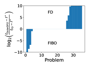
Figure 3.1: Log-ratio plot (3.1) comparing the final accuracy achieved by FIBO and FD.

In the next set of experiments, we measure the efficiency of FIBO by recording the number of objective and constraint evaluations required to achieve the accuracy

$$f(x_{k})\leq f^{*}+\tau\cdot\max(1,|f^{*}|),$$ (3.2)

for $\tau=10^{-1},10^{-3},10^{-5}$ and $10^{-7}$. We denote by $\text{evals}_{\text{FIBO}}$ and $\text{evals}_{\text{FD}}$ the number of objective function evaluations required by each method to satisfy (3.2). Similarly, $\text{cevals}_{\text{FIBO}}$ and $\text{cevals}_{\text{FD}}$ denote the number of constraint evaluations. If condition (3.2) cannot be satisfied by an algorithm, we set the corresponding quantity as a very large number. We summarize the performance of IBO and FD in Figures 3.2 and 3.3, respectively, by reporting the log-ratios

$$\log_{2}\left(\frac{\text{evals}_{\text{FIBO}}}{\text{evals}_{\text{FD}}}\right),\quad\log_{2}\left(\frac{\text{cevals}_{\text{FIBO}}}{\text{cevals}_{\text{FD}}}\right).$$ (3.3)

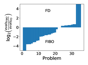
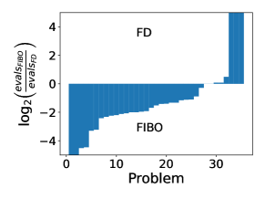
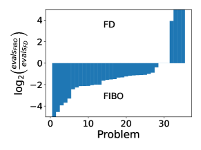
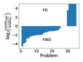
Figure 3.2: Log-ratio plot comparing FIBO and FD in terms of the number of objective function evaluations required to satisfy (3.2) for $\tau=10^{-1}\text{ (upper left)},$ $10^{-3}\text{ (upper right)},\\$ $10^{-5}$ $\text{ (bottom left)},10^{-7}\text{ (bottom right)}$.

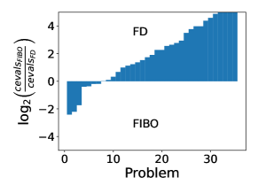
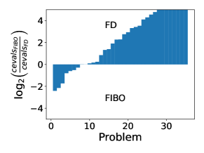
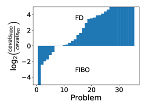
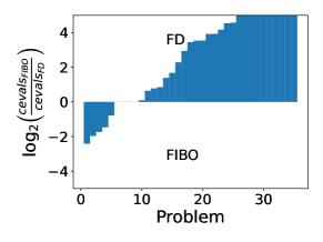
Figure 3.3: Log-ratio plot comparing FIBO and FD in terms of the number of constraint evaluations to satisfy (3.2) for $\tau=10^{-1}\text{ (upper left)}$, $10^{-3}\text{ (upper right)},$ $10^{-5}\text{ (bottom left)}$, $10^{-7}\text{ (bottom right)}$.

As shown in Figure 3.2, FIBO outperforms FD in terms of objective evaluations across all accuracy levels, while FD is far more efficient in terms of constraint evaluations, as expected. This provides support for the claim that FIBO is well-suited for problems in which the cost of the objective function dominates all other costs.

4 Final Remarks

In this paper, we studied the numerical efficiency of the feasible interpolation-based optimization (FIBO) approach first proposed by Conn, Scheinberg and Toint [6] for constrained optimization problems in which the gradient of the objective function is not available. While this method has been examined in previous studies [6, 4, 2], none of them provided compelling numerical evidence regarding its practical viability. To the best of our knowledge, this method is rarely, if ever, utilized in practical applications, a situation this article attempts to rectify. Our numerical tests indicate that FIBO is a very competitive method for solving problems where the evaluation of the objective function $f$ dominates the cost of solving the trust region problem (2.4). This implies, in particular, that the evaluations of the constraints and their derivatives must be very inexpensive compared to the evaluation of $f$. This is the case when $f$ is the result of an expensive simulation while the constraints are provided analytically. Note, however, that FIBO does not require that the derivatives of the constraints be provided analytically; they could be approximated by finite differences. The only requirement is that these computations be inexpensive compared to an evaluation of $f$.

The primary limitation of FIBO lies in the need to solve the nonlinear programming subproblem (2.4) to optimality at each iteration. Although we never encountered failures in our experiments, it cannot be assured that an optimal solution of this subproblem is always found.

In this paper, we have not explored scenarios in which the objective function exhibits noise. Nonetheless, it is our expectation that the FIBO approach will be effective in such conditions too. This view is based in the empirically observed robustness of the IBO strategy to noise, as reported by Shi et al. [25].

Appendix A Numerical Results for Feasible Initial Points

			FIBO								knitro
Problem	n	m	#iter	#feval	time	$f$	feas err	#iter(sub)	#ceval	time(sub)	#iter	#feval	time	$f$	feas err
HS13	$2$	$1$	$3$	$5$	$0.29$	$1.000\text{\times}{10}^{00}$	$1.309\text{\times}{10}^{-14}$	136	191	0.28	$20$	$104$	$0.09$	$9.983\text{\times}{10}^{-01}$	$6.579\text{\times}{10}^{-10}$
HS22	$2$	$2$	$2$	$4$	$0.04$	$1.000\text{\times}{10}^{00}$	$0.000\text{\times}{10}^{00}$	10	25	0.03	$1$	$8$	$0.01$	$1.000\text{\times}{10}^{00}$	$0.000\text{\times}{10}^{00}$
HS23	$2$	$5$	$4$	$6$	$0.04$	$2.000\text{\times}{10}^{00}$	$0.000\text{\times}{10}^{00}$	12	16	0.03	$6$	$28$	$0.03$	$2.000\text{\times}{10}^{00}$	$0.000\text{\times}{10}^{00}$
HS26	$3$	$1$	$53$	$56$	$12.96$	$7.103\text{\times}{10}^{-10}$	$2.220\text{\times}{10}^{-16}$	5245	39137	12.85	$34$	$244$	$0.1$	$7.434\text{\times}{10}^{-12}$	$6.661\text{\times}{10}^{-16}$
HS32	$3$	$2$	$4$	$7$	$0.04$	$1.000\text{\times}{10}^{00}$	$0.000\text{\times}{10}^{00}$	10	16	0.03	$2$	$15$	$0.01$	$1.000\text{\times}{10}^{00}$	$0.000\text{\times}{10}^{00}$
HS34	$3$	$2$	$6$	$9$	$0.1$	$-8.340\text{\times}{10}^{-01}$	$1.776\text{\times}{10}^{-15}$	32	70	0.08	$7$	$44$	$0.02$	$-8.340\text{\times}{10}^{-01}$	$0.000\text{\times}{10}^{00}$
HS40	$4$	$3$	$22$	$26$	$0.36$	$-2.500\text{\times}{10}^{-01}$	$1.110\text{\times}{10}^{-16}$	56	225	0.26	$5$	$44$	$0.01$	$-2.500\text{\times}{10}^{-01}$	$1.110\text{\times}{10}^{-16}$
HS44	$4$	$6$	$3$	$8$	$0.04$	$-1.000\text{\times}{10}^{00}$(*)	$0.000\text{\times}{10}^{00}$	12	23	0.03	$5$	$36$	$0.03$	$-1.500\text{\times}{10}^{01}$	$0.000\text{\times}{10}^{00}$
HS47	$5$	$3$	$23$	$28$	$3.67$	$1.989\text{\times}{10}^{-07}$	$3.781\text{\times}{10}^{-11}$	1391	7878	3.47	$72$	$696$	$0.41$	$1.007\text{\times}{10}^{01}$	$6.661\text{\times}{10}^{-16}$
HS50	$5$	$3$	$19$	$24$	$1.17$	$1.056\text{\times}{10}^{00}$	$2.398\text{\times}{10}^{-14}$	126	423	1.1	$16$	$121$	$0.04$	$7.669\text{\times}{10}^{-17}$	$4.441\text{\times}{10}^{-16}$
HS64	$3$	$1$	$43$	$46$	$1.04$	$6.300\text{\times}{10}^{03}$	$0.000\text{\times}{10}^{00}$	300	662	0.95	$12$	$65$	$0.04$	$6.300\text{\times}{10}^{03}$	$0.000\text{\times}{10}^{00}$
HS66	$3$	$2$	$2$	$6$	$0.03$	$5.182\text{\times}{10}^{-01}$(*)	$3.563\text{\times}{10}^{-12}$	7	12	0.02	$7$	$43$	$0.03$	$5.182\text{\times}{10}^{-01}$	$0.000\text{\times}{10}^{00}$
HS67	$3$	$14$	$45$	$49$	$1.7$	$-1.162\text{\times}{10}^{03}$(*)	$0.000\text{\times}{10}^{00}$	472	1408	1.59	$14$	$75$	$0.03$	$-1.162\text{\times}{10}^{03}$	$0.000\text{\times}{10}^{00}$
HS72	$4$	$2$	$7$	$11$	$0.26$	$7.277\text{\times}{10}^{02}$	$2.819\text{\times}{10}^{-18}$	44	99	0.21	$8$	$55$	$0.03$	$7.277\text{\times}{10}^{02}$	$4.337\text{\times}{10}^{-19}$
HS75	$4$	$5$	$16$	$20$	$0.49$	$5.174\text{\times}{10}^{03}$	$5.684\text{\times}{10}^{-14}$	97	180	0.43	$6$	$43$	$0.04$	$5.174\text{\times}{10}^{03}$	$8.527\text{\times}{10}^{-14}$
HS85	$5$	$21$	$31$	$36$	$1.46$	$-2.216\text{\times}{10}^{00}$	$0.000\text{\times}{10}^{00}$	357	903	1.31	$11$	$85$	$0.06$	$-2.216\text{\times}{10}^{00}$	$1.421\text{\times}{10}^{-14}$
HS87	$6$	$4$	$9$	$15$	$0.74$	$8.997\text{\times}{10}^{03}$	$2.274\text{\times}{10}^{-13}$	80	287	0.71	$14$	$223$	$0.07$	$8.997\text{\times}{10}^{03}$	$2.416\text{\times}{10}^{-13}$
HS88	$2$	$1$	$5$	$7$	$0.4$	$1.363\text{\times}{10}^{00}$	$0.000\text{\times}{10}^{00}$	92	318	0.39	$27$	$156$	$0.08$	$1.363\text{\times}{10}^{00}$	$2.893\text{\times}{10}^{-17}$
HS89	$3$	$1$	$10$	$13$	$1.42$	$1.363\text{\times}{10}^{00}$	$0.000\text{\times}{10}^{00}$	246	889	1.39	$5$	$35$	$0.04$	$7.283\text{\times}{10}^{-08}$$(\dagger)$	$1.332\text{\times}{10}^{-01}$
HS90	$4$	$1$	$12$	$16$	$4.22$	$1.363\text{\times}{10}^{00}$	$0.000\text{\times}{10}^{00}$	738	3531	4.18	$33$	$285$	$0.15$	$1.363\text{\times}{10}^{00}$	$6.600\text{\times}{10}^{-18}$
HS93	$6$	$2$	$42$	$48$	$2.9$	$1.351\text{\times}{10}^{02}$	$4.800\text{\times}{10}^{-12}$	517	2433	2.61	$26$	$295$	$0.13$	$1.351\text{\times}{10}^{02}$	$0.000\text{\times}{10}^{00}$
HS98	$6$	$4$	$3$	$10$	$0.05$	$3.136\text{\times}{10}^{00}$(*)	$1.776\text{\times}{10}^{-15}$	5	8	0.02	$4$	$40$	$0.02$	$3.136\text{\times}{10}^{00}$	$1.776\text{\times}{10}^{-15}$
HS100	$7$	$4$	$106$	$113$	$29.46$	$6.806\text{\times}{10}^{02}$	$0.000\text{\times}{10}^{00}$	3280	22448	28.72	$51$	$587$	$0.21$	$6.806\text{\times}{10}^{02}$	$7.161\text{\times}{10}^{-15}$
HS101	$7$	$5$	$103$	$110$	$19.42$	$1.810\text{\times}{10}^{03}$	$3.955\text{\times}{10}^{-16}$	2616	15697	18.39	$35$	$354$	$0.19$	$1.810\text{\times}{10}^{03}$	$0.000\text{\times}{10}^{00}$
HS102	$7$	$5$	$103$	$110$	$15.11$	$9.119\text{\times}{10}^{02}$	$3.816\text{\times}{10}^{-16}$	1985	10240	13.86	$21$	$254$	$0.13$	$9.119\text{\times}{10}^{02}$	$2.498\text{\times}{10}^{-16}$
HS103	$7$	$5$	$56$	$63$	$5.5$	$5.437\text{\times}{10}^{02}$	$1.318\text{\times}{10}^{-16}$	825	4072	4.59	$20$	$238$	$0.1$	$5.437\text{\times}{10}^{02}$	$2.359\text{\times}{10}^{-16}$
HS104	$8$	$5$	$245$	$253$	$43.5$	$3.951\text{\times}{10}^{00}$	$9.714\text{\times}{10}^{-17}$	6813	37268	41.25	$30$	$359$	$0.1$	$3.951\text{\times}{10}^{00}$	$2.082\text{\times}{10}^{-16}$
LOADBAL	$31$	$31$	$1$	$15499$	$0.93$	$1.547\text{\times}{10}^{00}$(***)	$1.798\text{\times}{10}^{308}$	0	1	0.0	$40$	$1380$	$0.21$	$4.529\text{\times}{10}^{-01}$	$2.665\text{\times}{10}^{-15}$
OPTPRLOC	$30$	$30$	$9$	$39$	$1.0$	$-1.642\text{\times}{10}^{01}$	$1.990\text{\times}{10}^{-13}$	54	127	0.45	$16$	$583$	$0.13$	$-1.642\text{\times}{10}^{01}$	$1.421\text{\times}{10}^{-13}$
CB3	$3$	$3$	$1$	$4$	$0.01$	$2.000\text{\times}{10}^{00}$	$0.000\text{\times}{10}^{00}$	2	3	0.0	$2$	$15$	$0.01$	$2.000\text{\times}{10}^{00}$	$0.000\text{\times}{10}^{00}$
CRESC50	$6$	$100$	$1000$	$1006$	$215.01$	$5.939\text{\times}{10}^{-01}$(**)	$5.482\text{\times}{10}^{-13}$	26160	96691	210.07	$438$	$5787$	$1.76$	$5.946\text{\times}{10}^{-01}$	$1.188\text{\times}{10}^{-14}$
DEMBO7	$16$	$20$	$19$	$35$	$2.37$	$1.748\text{\times}{10}^{02}$	$4.073\text{\times}{10}^{-15}$	302	795	2.07	$17$	$354$	$0.16$	$1.749\text{\times}{10}^{02}$	$6.661\text{\times}{10}^{-16}$
DNIEPER	$57$	$24$	$24$	$81$	$7.72$	$1.874\text{\times}{10}^{04}$	$5.684\text{\times}{10}^{-14}$	273	1094	3.25	$8$	$534$	$0.11$	$1.874\text{\times}{10}^{04}$	$5.684\text{\times}{10}^{-14}$
EXPFITA	$5$	$22$	$1$	$10999$	$0.6$	$2.999\text{\times}{10}^{01}$(***)	$1.798\text{\times}{10}^{308}$	0	1	0.0	$19$	$140$	$0.05$	$1.137\text{\times}{10}^{-03}$	$1.421\text{\times}{10}^{-14}$
HIMMELBI	$100$	$12$	$114$	$215$	$72.23$	$-1.467\text{\times}{10}^{03}$(*)	$1.789\text{\times}{10}^{-09}$	2618	12586	67.95	$72$	$7487$	$0.72$	$-1.736\text{\times}{10}^{03}$	$1.066\text{\times}{10}^{-14}$
SYNTHES1	$6$	$6$	$1$	$2999$	$0.21$	$1.000\text{\times}{10}^{01}$(***)	$1.798\text{\times}{10}^{308}$	0	1	0.0	$9$	$81$	$0.03$	$7.593\text{\times}{10}^{-01}$	$1.110\text{\times}{10}^{-16}$
TWOBARS	$2$	$2$	$7$	$9$	$0.1$	$1.509\text{\times}{10}^{00}$	$0.000\text{\times}{10}^{00}$	24	108	0.09	$9$	$57$	$0.03$	$1.509\text{\times}{10}^{00}$	$4.441\text{\times}{10}^{-16}$
DIPIGRI	$7$	$4$	$116$	$123$	$85.85$	$6.806\text{\times}{10}^{02}$	$3.581\text{\times}{10}^{-11}$	7461	26264	84.59	$48$	$581$	$0.18$	$6.806\text{\times}{10}^{02}$	$0.000\text{\times}{10}^{00}$

Table A.1: Noiseless Problems with Feasible $x_{0}$; $n$: number of variables, $m$: number of constraints, #iter: number of (outer) iterations, #feval: number of function evaluations, time: total CPU time passed, $f$: final objective value, feas err: final feasibility error, #iter(sub): total number of iterations for solving TR subproblem, #ceval: total number of constraint evaluations(note that the number of constraint evaluations and function evaluations are same for KNITRO), time(sub): total CPU time elapsed for solving subproblem. * indicates that FIBO terminates with singular interpolation system error, ** indicates that FIBO terminates with maximum number of iterations, *** indicates that FIBO terminates with maximum number of function evaluations.

			FIBO								knitro
Problem	n	m	#iter	#feval	time	$f$	feas err	#iter(sub)	#ceval	time(sub)	#iter	#feval	time	$f$	feas err
HS13	$2$	$1$	$2$	$4$	$0.2$	$1.000\text{\times}{10}^{00}$	$1.310\text{\times}{10}^{-14}$	75	104	0.19	$8$	$36$	$0.02$	$1.080\text{\times}{10}^{00}$	$0.000\text{\times}{10}^{00}$
HS22	$2$	$2$	$1$	$3$	$0.03$	$1.000\text{\times}{10}^{00}$	$1.789\text{\times}{10}^{-12}$	9	23	0.02	$0$	$3$	$0.0$	$1.000\text{\times}{10}^{00}$	$1.843\text{\times}{10}^{-14}$
HS23	$2$	$5$	$3$	$5$	$0.05$	$2.000\text{\times}{10}^{00}$	$0.000\text{\times}{10}^{00}$	11	14	0.03	$3$	$16$	$0.01$	$2.040\text{\times}{10}^{00}$	$0.000\text{\times}{10}^{00}$
HS26	$3$	$1$	$4$	$7$	$0.09$	$1.996\text{\times}{10}^{-02}$	$9.592\text{\times}{10}^{-14}$	32	66	0.07	$14$	$87$	$0.04$	$4.252\text{\times}{10}^{-07}$	$9.633\text{\times}{10}^{-07}$
HS32	$3$	$2$	$4$	$7$	$0.09$	$1.000\text{\times}{10}^{00}$	$0.000\text{\times}{10}^{00}$	10	16	0.04	$2$	$15$	$0.02$	$1.000\text{\times}{10}^{00}$	$0.000\text{\times}{10}^{00}$
HS34	$3$	$2$	$5$	$8$	$0.09$	$-7.820\text{\times}{10}^{-01}$	$1.066\text{\times}{10}^{-14}$	31	68	0.08	$4$	$29$	$0.02$	$-8.266\text{\times}{10}^{-01}$	$0.000\text{\times}{10}^{00}$
HS40	$4$	$3$	$1$	$5$	$0.02$	$-2.454\text{\times}{10}^{-01}$	$2.554\text{\times}{10}^{-15}$	5	15	0.01	$0$	$4$	$0.0$	$-2.454\text{\times}{10}^{-01}$	$7.334\text{\times}{10}^{-09}$
HS44	$4$	$6$	$3$	$8$	$0.09$	$-1.000\text{\times}{10}^{00}$(*)	$0.000\text{\times}{10}^{00}$	12	23	0.07	$4$	$30$	$0.02$	$-1.500\text{\times}{10}^{01}$	$0.000\text{\times}{10}^{00}$
HS47	$5$	$3$	$6$	$11$	$0.14$	$5.639\text{\times}{10}^{-02}$	$1.466\text{\times}{10}^{-12}$	46	118	0.12	$17$	$134$	$0.04$	$4.638\text{\times}{10}^{-08}$	$3.167\text{\times}{10}^{-09}$
HS50	$5$	$3$	$19$	$24$	$1.26$	$1.056\text{\times}{10}^{00}$	$2.398\text{\times}{10}^{-14}$	126	423	1.19	$9$	$71$	$0.03$	$4.941\text{\times}{10}^{-02}$	$4.441\text{\times}{10}^{-16}$
HS64	$3$	$1$	$1$	$4$	$0.05$	$6.813\text{\times}{10}^{03}$	$4.742\text{\times}{10}^{-11}$	14	72	0.05	$0$	$3$	$0.0$	$6.813\text{\times}{10}^{03}$	$0.000\text{\times}{10}^{00}$
HS66	$3$	$2$	$1$	$4$	$0.02$	$5.800\text{\times}{10}^{-01}$	$3.563\text{\times}{10}^{-12}$	6	10	0.01	$0$	$3$	$0.0$	$5.800\text{\times}{10}^{-01}$	$0.000\text{\times}{10}^{00}$
HS67	$3$	$14$	$31$	$34$	$1.91$	$-1.053\text{\times}{10}^{03}$	$0.000\text{\times}{10}^{00}$	402	1319	1.82	$8$	$45$	$0.02$	$-1.157\text{\times}{10}^{03}$	$0.000\text{\times}{10}^{00}$
HS72	$4$	$2$	$1$	$5$	$0.01$	$7.407\text{\times}{10}^{02}$	$0.000\text{\times}{10}^{00}$	2	5	0.01	$0$	$4$	$0.0$	$7.407\text{\times}{10}^{02}$	$0.000\text{\times}{10}^{00}$
HS75	$4$	$5$	$1$	$5$	$0.02$	$5.350\text{\times}{10}^{03}$	$1.259\text{\times}{10}^{-08}$	4	8	0.01	$5$	$37$	$0.03$	$5.174\text{\times}{10}^{03}$	$7.739\text{\times}{10}^{-08}$
HS85	$5$	$21$	$29$	$34$	$1.22$	$-2.061\text{\times}{10}^{00}$	$1.421\text{\times}{10}^{-14}$	348	880	1.04	$10$	$78$	$0.05$	$-2.216\text{\times}{10}^{00}$	$2.389\text{\times}{10}^{-08}$
HS87	$6$	$4$	$1$	$7$	$0.07$	$8.997\text{\times}{10}^{03}$	$2.274\text{\times}{10}^{-13}$	9	24	0.06	$0$	$5$	$0.0$	$8.997\text{\times}{10}^{03}$	$2.956\text{\times}{10}^{-12}$
HS88	$2$	$1$	$1$	$3$	$0.07$	$1.385\text{\times}{10}^{00}$	$2.158\text{\times}{10}^{-14}$	19	41	0.07	$0$	$3$	$0.0$	$1.385\text{\times}{10}^{00}$	$0.000\text{\times}{10}^{00}$
HS89	$3$	$1$	$2$	$5$	$0.29$	$1.365\text{\times}{10}^{00}$	$1.123\text{\times}{10}^{-16}$	57	205	0.28	$5$	$35$	$0.03$	$7.283\text{\times}{10}^{-08}$$(\dagger)$	$1.332\text{\times}{10}^{-01}$
HS90	$4$	$1$	$2$	$6$	$0.53$	$1.446\text{\times}{10}^{00}$	$6.661\text{\times}{10}^{-16}$	86	454	0.52	$24$	$228$	$0.11$	$1.362\text{\times}{10}^{00}$	$5.472\text{\times}{10}^{-07}$
HS93	$6$	$2$	$1$	$7$	$0.11$	$1.371\text{\times}{10}^{02}$	$2.946\text{\times}{10}^{-11}$	10	24	0.11	$0$	$5$	$0.0$	$1.371\text{\times}{10}^{02}$	$0.000\text{\times}{10}^{00}$
HS98	$6$	$4$	$2$	$8$	$0.03$	$3.136\text{\times}{10}^{00}$	$0.000\text{\times}{10}^{00}$	4	6	0.02	$3$	$32$	$0.02$	$3.136\text{\times}{10}^{00}$	$0.000\text{\times}{10}^{00}$
HS100	$7$	$4$	$1$	$8$	$0.12$	$7.140\text{\times}{10}^{02}$	$0.000\text{\times}{10}^{00}$	22	79	0.12	$0$	$5$	$0.0$	$7.140\text{\times}{10}^{02}$	$0.000\text{\times}{10}^{00}$
HS101	$7$	$5$	$26$	$33$	$5.24$	$1.982\text{\times}{10}^{03}$	$3.053\text{\times}{10}^{-16}$	740	4383	5.04	$9$	$106$	$0.04$	$1.848\text{\times}{10}^{03}$	$0.000\text{\times}{10}^{00}$
HS102	$7$	$5$	$34$	$41$	$4.55$	$9.948\text{\times}{10}^{02}$	$2.776\text{\times}{10}^{-17}$	641	3320	4.29	$11$	$159$	$0.05$	$9.191\text{\times}{10}^{02}$	$0.000\text{\times}{10}^{00}$
HS103	$7$	$5$	$15$	$22$	$1.69$	$5.623\text{\times}{10}^{02}$	$8.913\text{\times}{10}^{-12}$	276	1263	1.63	$16$	$202$	$0.06$	$5.437\text{\times}{10}^{02}$	$1.040\text{\times}{10}^{-07}$
HS104	$8$	$5$	$1$	$9$	$0.11$	$4.200\text{\times}{10}^{00}$	$1.459\text{\times}{10}^{-11}$	14	41	0.11	$0$	$6$	$0.0$	$4.200\text{\times}{10}^{00}$	$0.000\text{\times}{10}^{00}$
LOADBAL	$31$	$31$	$1$	$15499$	$0.97$	$1.547\text{\times}{10}^{00}$(***)	$1.798\text{\times}{10}^{308}$	0	1	0.0	$6$	$231$	$0.04$	$5.252\text{\times}{10}^{-01}$	$1.710\text{\times}{10}^{-14}$
OPTPRLOC	$30$	$30$	$5$	$35$	$0.46$	$-1.567\text{\times}{10}^{01}$	$2.220\text{\times}{10}^{-16}$	44	104	0.4	$2$	$103$	$0.04$	$-1.587\text{\times}{10}^{01}$	$6.661\text{\times}{10}^{-16}$
CB3	$3$	$3$	$1$	$4$	$0.01$	$2.000\text{\times}{10}^{00}$	$0.000\text{\times}{10}^{00}$	2	3	0.01	$1$	$10$	$0.01$	$2.000\text{\times}{10}^{00}$	$7.270\text{\times}{10}^{-13}$
CRESC50	$6$	$100$	$16$	$22$	$2.44$	$6.057\text{\times}{10}^{-01}$	$9.032\text{\times}{10}^{-11}$	344	1528	2.38	$58$	$700$	$0.32$	$6.155\text{\times}{10}^{-01}$	$0.000\text{\times}{10}^{00}$
DEMBO7	$16$	$20$	$13$	$29$	$1.39$	$1.879\text{\times}{10}^{02}$	$5.917\text{\times}{10}^{-08}$	198	507	1.19	$15$	$318$	$0.1$	$1.749\text{\times}{10}^{02}$	$1.869\text{\times}{10}^{-13}$
DNIEPER	$57$	$24$	$4$	$61$	$1.82$	$1.941\text{\times}{10}^{04}$	$4.264\text{\times}{10}^{-11}$	96	457	1.35	$2$	$177$	$0.03$	$1.874\text{\times}{10}^{04}$	$1.800\text{\times}{10}^{-07}$
EXPFITA	$5$	$22$	$1$	$10999$	$0.61$	$2.999\text{\times}{10}^{01}$(***)	$1.798\text{\times}{10}^{308}$	0	1	0.0	$7$	$56$	$0.02$	$9.889\text{\times}{10}^{-02}$	$1.354\text{\times}{10}^{-14}$
HIMMELBI	$100$	$12$	$114$	$215$	$70.47$	$-1.467\text{\times}{10}^{03}$(*)	$1.789\text{\times}{10}^{-09}$	2618	12586	68.05	$3$	$408$	$0.09$	$-1.643\text{\times}{10}^{03}$	$0.000\text{\times}{10}^{00}$
SYNTHES1	$6$	$6$	$1$	$2999$	$0.22$	$1.000\text{\times}{10}^{01}$(***)	$1.798\text{\times}{10}^{308}$	0	1	0.0	$7$	$65$	$0.02$	$7.593\text{\times}{10}^{-01}$	$3.261\text{\times}{10}^{-07}$
TWOBARS	$2$	$2$	$2$	$4$	$0.05$	$1.523\text{\times}{10}^{00}$	$7.885\text{\times}{10}^{-09}$	13	38	0.04	$7$	$49$	$0.05$	$1.509\text{\times}{10}^{00}$	$2.179\text{\times}{10}^{-09}$
DIPIGRI	$7$	$4$	$1$	$8$	$0.14$	$7.140\text{\times}{10}^{02}$	$0.000\text{\times}{10}^{00}$	22	79	0.13	$0$	$5$	$0.0$	$7.140\text{\times}{10}^{02}$	$0.000\text{\times}{10}^{00}$

Table A.2: Noiseless Problems with Feasible $x_{0}$. $\tau=10^{-1}$; $n$: number of variables, $m$: number of constraints, #iter: number of (outer) iterations, #feval: number of function evaluations, time: total CPU time passed, $f$: final objective value, feas err: final feasibility error, #iter(sub): total number of iterations for solving TR subproblem, #ceval: total number of constraint evaluations(note that the number of constraint evaluations and function evaluations are same for KNITRO), time(sub): total CPU time elapsed for solving subproblem. * indicates that FIBO terminates with singular interpolation system error, ** indicates that FIBO terminates with maximum number of iterations, *** indicates that FIBO terminates with maximum number of function evaluations.

			FIBO								knitro
Problem	n	m	#iter	#feval	time	$f$	feas err	#iter(sub)	#ceval	time(sub)	#iter	#feval	time	$f$	feas err
HS13	$2$	$1$	$2$	$4$	$0.18$	$1.000\text{\times}{10}^{00}$	$1.310\text{\times}{10}^{-14}$	75	104	0.17	$18$	$88$	$0.08$	$1.001\text{\times}{10}^{00}$	$0.000\text{\times}{10}^{00}$
HS22	$2$	$2$	$1$	$3$	$0.03$	$1.000\text{\times}{10}^{00}$	$1.789\text{\times}{10}^{-12}$	9	23	0.02	$0$	$3$	$0.0$	$1.000\text{\times}{10}^{00}$	$1.843\text{\times}{10}^{-14}$
HS23	$2$	$5$	$3$	$5$	$0.04$	$2.000\text{\times}{10}^{00}$	$0.000\text{\times}{10}^{00}$	11	14	0.03	$4$	$20$	$0.02$	$2.000\text{\times}{10}^{00}$	$0.000\text{\times}{10}^{00}$
HS26	$3$	$1$	$36$	$39$	$1.85$	$1.737\text{\times}{10}^{-04}$	$1.040\text{\times}{10}^{-12}$	754	4338	1.77	$14$	$87$	$0.03$	$4.252\text{\times}{10}^{-07}$	$9.633\text{\times}{10}^{-07}$
HS32	$3$	$2$	$4$	$7$	$0.05$	$1.000\text{\times}{10}^{00}$	$0.000\text{\times}{10}^{00}$	10	16	0.03	$2$	$15$	$0.02$	$1.000\text{\times}{10}^{00}$	$0.000\text{\times}{10}^{00}$
HS34	$3$	$2$	$6$	$9$	$0.11$	$-8.340\text{\times}{10}^{-01}$	$1.776\text{\times}{10}^{-15}$	32	70	0.08	$6$	$39$	$0.01$	$-8.340\text{\times}{10}^{-01}$	$5.446\text{\times}{10}^{-09}$
HS40	$4$	$3$	$2$	$6$	$0.03$	$-2.491\text{\times}{10}^{-01}$	$2.189\text{\times}{10}^{-09}$	8	21	0.02	$3$	$32$	$0.02$	$-2.500\text{\times}{10}^{-01}$	$2.040\text{\times}{10}^{-09}$
HS44	$4$	$6$	$3$	$8$	$0.05$	$-1.000\text{\times}{10}^{00}$(*)	$0.000\text{\times}{10}^{00}$	12	23	0.03	$4$	$30$	$0.03$	$-1.500\text{\times}{10}^{01}$	$0.000\text{\times}{10}^{00}$
HS47	$5$	$3$	$23$	$28$	$3.41$	$1.989\text{\times}{10}^{-07}$	$3.781\text{\times}{10}^{-11}$	1391	7878	3.33	$72$	$696$	$0.35$	$1.007\text{\times}{10}^{01}$	$6.661\text{\times}{10}^{-16}$
HS50	$5$	$3$	$19$	$24$	$1.02$	$1.056\text{\times}{10}^{00}$	$2.398\text{\times}{10}^{-14}$	126	423	0.96	$11$	$85$	$0.03$	$1.339\text{\times}{10}^{-06}$	$8.882\text{\times}{10}^{-16}$
HS64	$3$	$1$	$13$	$16$	$0.46$	$6.303\text{\times}{10}^{03}$	$1.443\text{\times}{10}^{-15}$	126	399	0.44	$7$	$40$	$0.02$	$6.300\text{\times}{10}^{03}$	$7.051\text{\times}{10}^{-10}$
HS66	$3$	$2$	$2$	$5$	$0.02$	$5.182\text{\times}{10}^{-01}$	$3.563\text{\times}{10}^{-12}$	7	12	0.02	$3$	$21$	$0.02$	$5.186\text{\times}{10}^{-01}$	$0.000\text{\times}{10}^{00}$
HS67	$3$	$14$	$38$	$41$	$1.51$	$-1.162\text{\times}{10}^{03}$	$0.000\text{\times}{10}^{00}$	448	1377	1.42	$9$	$50$	$0.02$	$-1.161\text{\times}{10}^{03}$	$0.000\text{\times}{10}^{00}$
HS72	$4$	$2$	$5$	$9$	$0.17$	$7.284\text{\times}{10}^{02}$	$0.000\text{\times}{10}^{00}$	38	90	0.16	$3$	$24$	$0.02$	$7.277\text{\times}{10}^{02}$	$1.663\text{\times}{10}^{-07}$
HS75	$4$	$5$	$16$	$20$	$0.32$	$5.174\text{\times}{10}^{03}$	$5.684\text{\times}{10}^{-14}$	97	180	0.28	$5$	$37$	$0.04$	$5.174\text{\times}{10}^{03}$	$7.739\text{\times}{10}^{-08}$
HS85	$5$	$21$	$31$	$36$	$0.95$	$-2.216\text{\times}{10}^{00}$	$0.000\text{\times}{10}^{00}$	357	903	0.87	$10$	$78$	$0.05$	$-2.216\text{\times}{10}^{00}$	$2.389\text{\times}{10}^{-08}$
HS87	$6$	$4$	$1$	$7$	$0.07$	$8.997\text{\times}{10}^{03}$	$2.274\text{\times}{10}^{-13}$	9	24	0.06	$0$	$5$	$0.0$	$8.997\text{\times}{10}^{03}$	$2.956\text{\times}{10}^{-12}$
HS88	$2$	$1$	$2$	$4$	$0.2$	$1.363\text{\times}{10}^{00}$	$9.216\text{\times}{10}^{-16}$	41	139	0.19	$23$	$140$	$0.06$	$1.362\text{\times}{10}^{00}$	$4.623\text{\times}{10}^{-07}$
HS89	$3$	$1$	$4$	$7$	$0.49$	$1.363\text{\times}{10}^{00}$	$3.663\text{\times}{10}^{-16}$	101	374	0.48	$5$	$35$	$0.04$	$7.283\text{\times}{10}^{-08}$$(\dagger)$	$1.332\text{\times}{10}^{-01}$
HS90	$4$	$1$	$6$	$10$	$1.54$	$1.363\text{\times}{10}^{00}$	$5.260\text{\times}{10}^{-17}$	277	1541	1.52	$24$	$228$	$0.14$	$1.362\text{\times}{10}^{00}$	$5.472\text{\times}{10}^{-07}$
HS93	$6$	$2$	$21$	$27$	$1.5$	$1.352\text{\times}{10}^{02}$	$4.695\text{\times}{10}^{-11}$	333	1706	1.43	$8$	$87$	$0.04$	$1.351\text{\times}{10}^{02}$	$0.000\text{\times}{10}^{00}$
HS98	$6$	$4$	$2$	$8$	$0.04$	$3.136\text{\times}{10}^{00}$	$0.000\text{\times}{10}^{00}$	4	6	0.01	$3$	$32$	$0.02$	$3.136\text{\times}{10}^{00}$	$0.000\text{\times}{10}^{00}$
HS100	$7$	$4$	$51$	$58$	$15.18$	$6.813\text{\times}{10}^{02}$	$1.388\text{\times}{10}^{-17}$	1609	11182	15.01	$3$	$55$	$0.02$	$6.811\text{\times}{10}^{02}$	$0.000\text{\times}{10}^{00}$
HS101	$7$	$5$	$44$	$51$	$7.81$	$1.812\text{\times}{10}^{03}$	$3.006\text{\times}{10}^{-10}$	1239	7244	7.65	$18$	$198$	$0.1$	$1.810\text{\times}{10}^{03}$	$2.139\text{\times}{10}^{-08}$
HS102	$7$	$5$	$69$	$76$	$10.13$	$9.125\text{\times}{10}^{02}$	$4.272\text{\times}{10}^{-13}$	1483	7663	9.89	$15$	$200$	$0.06$	$9.119\text{\times}{10}^{02}$	$5.354\text{\times}{10}^{-07}$
HS103	$7$	$5$	$37$	$44$	$3.94$	$5.437\text{\times}{10}^{02}$	$7.980\text{\times}{10}^{-16}$	671	3465	3.8	$16$	$202$	$0.08$	$5.437\text{\times}{10}^{02}$	$1.040\text{\times}{10}^{-07}$
HS104	$8$	$5$	$47$	$55$	$6.18$	$3.952\text{\times}{10}^{00}$	$5.218\text{\times}{10}^{-15}$	1210	6047	5.99	$20$	$259$	$0.05$	$3.951\text{\times}{10}^{00}$	$1.537\text{\times}{10}^{-07}$
LOADBAL	$31$	$31$	$1$	$15499$	$0.9$	$1.547\text{\times}{10}^{00}$(***)	$1.798\text{\times}{10}^{308}$	0	1	0.0	$9$	$330$	$0.05$	$4.531\text{\times}{10}^{-01}$	$1.421\text{\times}{10}^{-14}$
OPTPRLOC	$30$	$30$	$6$	$36$	$0.44$	$-1.642\text{\times}{10}^{01}$	$0.000\text{\times}{10}^{00}$	47	111	0.39	$3$	$136$	$0.06$	$-1.641\text{\times}{10}^{01}$	$0.000\text{\times}{10}^{00}$
CB3	$3$	$3$	$1$	$4$	$0.01$	$2.000\text{\times}{10}^{00}$	$0.000\text{\times}{10}^{00}$	2	3	0.01	$1$	$10$	$0.0$	$2.000\text{\times}{10}^{00}$	$7.270\text{\times}{10}^{-13}$
CRESC50	$6$	$100$	$68$	$74$	$18.0$	$5.942\text{\times}{10}^{-01}$	$0.000\text{\times}{10}^{00}$	2416	11257	17.76	$438$	$5787$	$1.81$	$5.946\text{\times}{10}^{-01}$	$1.188\text{\times}{10}^{-14}$
DEMBO7	$16$	$20$	$18$	$34$	$2.11$	$1.749\text{\times}{10}^{02}$	$1.067\text{\times}{10}^{-10}$	301	793	2.03	$15$	$318$	$0.1$	$1.749\text{\times}{10}^{02}$	$1.869\text{\times}{10}^{-13}$
DNIEPER	$57$	$24$	$5$	$62$	$1.42$	$1.874\text{\times}{10}^{04}$	$1.405\text{\times}{10}^{-09}$	100	465	1.35	$2$	$177$	$0.06$	$1.874\text{\times}{10}^{04}$	$1.800\text{\times}{10}^{-07}$
EXPFITA	$5$	$22$	$1$	$10999$	$0.58$	$2.999\text{\times}{10}^{01}$(***)	$1.798\text{\times}{10}^{308}$	0	1	0.0	$12$	$91$	$0.03$	$1.355\text{\times}{10}^{-03}$	$6.750\text{\times}{10}^{-14}$
HIMMELBI	$100$	$12$	$114$	$215$	$68.58$	$-1.467\text{\times}{10}^{03}$(*)	$1.789\text{\times}{10}^{-09}$	2618	12586	67.1	$12$	$1326$	$0.26$	$-1.734\text{\times}{10}^{03}$	$5.684\text{\times}{10}^{-14}$
SYNTHES1	$6$	$6$	$1$	$2999$	$0.21$	$1.000\text{\times}{10}^{01}$(***)	$1.798\text{\times}{10}^{308}$	0	1	0.0	$7$	$65$	$0.02$	$7.593\text{\times}{10}^{-01}$	$3.261\text{\times}{10}^{-07}$
TWOBARS	$2$	$2$	$3$	$5$	$0.06$	$1.509\text{\times}{10}^{00}$	$4.742\text{\times}{10}^{-11}$	16	55	0.05	$7$	$49$	$0.04$	$1.509\text{\times}{10}^{00}$	$2.179\text{\times}{10}^{-09}$
DIPIGRI	$7$	$4$	$51$	$58$	$11.33$	$6.812\text{\times}{10}^{02}$	$6.939\text{\times}{10}^{-18}$	1491	9509	11.16	$3$	$55$	$0.01$	$6.811\text{\times}{10}^{02}$	$0.000\text{\times}{10}^{00}$

Table A.3: Noiseless Problems with Feasible $x_{0}$. $\tau=10^{-3}$; $n$: number of variables, $m$: number of constraints, #iter: number of (outer) iterations, #feval: number of function evaluations, time: total CPU time passed, $f$: final objective value, feas err: final feasibility error, #iter(sub): total number of iterations for solving TR subproblem, #ceval: total number of constraint evaluations(note that the number of constraint evaluations and function evaluations are same for KNITRO), time(sub): total CPU time elapsed for solving subproblem. * indicates that FIBO terminates with singular interpolation system error, ** indicates that FIBO terminates with maximum number of iterations, *** indicates that FIBO terminates with maximum number of function evaluations.

			FIBO								knitro
Problem	n	m	#iter	#feval	time	$f$	feas err	#iter(sub)	#ceval	time(sub)	#iter	#feval	time	$f$	feas err
HS13	$2$	$1$	$3$	$5$	$0.29$	$1.000\text{\times}{10}^{00}$	$1.309\text{\times}{10}^{-14}$	136	191	0.28	$19$	$100$	$0.1$	$9.983\text{\times}{10}^{-01}$	$6.579\text{\times}{10}^{-10}$
HS22	$2$	$2$	$1$	$3$	$0.03$	$1.000\text{\times}{10}^{00}$	$1.789\text{\times}{10}^{-12}$	9	23	0.02	$0$	$3$	$0.0$	$1.000\text{\times}{10}^{00}$	$1.843\text{\times}{10}^{-14}$
HS23	$2$	$5$	$3$	$5$	$0.03$	$2.000\text{\times}{10}^{00}$	$0.000\text{\times}{10}^{00}$	11	14	0.02	$5$	$24$	$0.02$	$2.000\text{\times}{10}^{00}$	$0.000\text{\times}{10}^{00}$
HS26	$3$	$1$	$38$	$41$	$8.14$	$8.872\text{\times}{10}^{-07}$	$4.441\text{\times}{10}^{-16}$	3356	26976	8.07	$14$	$87$	$0.03$	$4.252\text{\times}{10}^{-07}$	$9.633\text{\times}{10}^{-07}$
HS32	$3$	$2$	$4$	$7$	$0.04$	$1.000\text{\times}{10}^{00}$	$0.000\text{\times}{10}^{00}$	10	16	0.03	$2$	$15$	$0.02$	$1.000\text{\times}{10}^{00}$	$0.000\text{\times}{10}^{00}$
HS34	$3$	$2$	$6$	$9$	$0.11$	$-8.340\text{\times}{10}^{-01}$	$1.776\text{\times}{10}^{-15}$	32	70	0.08	$6$	$39$	$0.01$	$-8.340\text{\times}{10}^{-01}$	$5.446\text{\times}{10}^{-09}$
HS40	$4$	$3$	$4$	$8$	$0.06$	$-2.500\text{\times}{10}^{-01}$	$1.058\text{\times}{10}^{-12}$	13	32	0.04	$3$	$32$	$0.03$	$-2.500\text{\times}{10}^{-01}$	$2.040\text{\times}{10}^{-09}$
HS44	$4$	$6$	$3$	$8$	$0.05$	$-1.000\text{\times}{10}^{00}$(*)	$0.000\text{\times}{10}^{00}$	12	23	0.04	$4$	$30$	$0.02$	$-1.500\text{\times}{10}^{01}$	$0.000\text{\times}{10}^{00}$
HS47	$5$	$3$	$23$	$28$	$3.42$	$1.989\text{\times}{10}^{-07}$	$3.781\text{\times}{10}^{-11}$	1391	7878	3.35	$72$	$696$	$0.38$	$1.007\text{\times}{10}^{01}$	$6.661\text{\times}{10}^{-16}$
HS50	$5$	$3$	$19$	$24$	$1.11$	$1.056\text{\times}{10}^{00}$	$2.398\text{\times}{10}^{-14}$	126	423	1.06	$11$	$85$	$0.04$	$1.339\text{\times}{10}^{-06}$	$8.882\text{\times}{10}^{-16}$
HS64	$3$	$1$	$17$	$20$	$0.55$	$6.300\text{\times}{10}^{03}$	$0.000\text{\times}{10}^{00}$	156	435	0.52	$7$	$40$	$0.02$	$6.300\text{\times}{10}^{03}$	$7.051\text{\times}{10}^{-10}$
HS66	$3$	$2$	$2$	$5$	$0.03$	$5.182\text{\times}{10}^{-01}$	$3.563\text{\times}{10}^{-12}$	7	12	0.02	$4$	$27$	$0.02$	$5.182\text{\times}{10}^{-01}$	$0.000\text{\times}{10}^{00}$
HS67	$3$	$14$	$39$	$42$	$1.45$	$-1.162\text{\times}{10}^{03}$	$0.000\text{\times}{10}^{00}$	450	1380	1.38	$10$	$55$	$0.03$	$-1.162\text{\times}{10}^{03}$	$0.000\text{\times}{10}^{00}$
HS72	$4$	$2$	$6$	$10$	$0.24$	$7.277\text{\times}{10}^{02}$	$6.263\text{\times}{10}^{-14}$	43	97	0.22	$4$	$31$	$0.02$	$7.277\text{\times}{10}^{02}$	$1.572\text{\times}{10}^{-10}$
HS75	$4$	$5$	$16$	$20$	$0.31$	$5.174\text{\times}{10}^{03}$	$5.684\text{\times}{10}^{-14}$	97	180	0.27	$5$	$37$	$0.03$	$5.174\text{\times}{10}^{03}$	$7.739\text{\times}{10}^{-08}$
HS85	$5$	$21$	$31$	$36$	$0.92$	$-2.216\text{\times}{10}^{00}$	$0.000\text{\times}{10}^{00}$	357	903	0.83	$10$	$78$	$0.05$	$-2.216\text{\times}{10}^{00}$	$2.389\text{\times}{10}^{-08}$
HS87	$6$	$4$	$2$	$8$	$0.11$	$8.997\text{\times}{10}^{03}$	$7.844\text{\times}{10}^{-12}$	15	43	0.1	$3$	$33$	$0.03$	$8.997\text{\times}{10}^{03}$	$2.396\text{\times}{10}^{-08}$
HS88	$2$	$1$	$4$	$6$	$0.31$	$1.363\text{\times}{10}^{00}$	$1.301\text{\times}{10}^{-14}$	69	218	0.3	$23$	$140$	$0.08$	$1.362\text{\times}{10}^{00}$	$4.623\text{\times}{10}^{-07}$
HS89	$3$	$1$	$5$	$8$	$0.55$	$1.363\text{\times}{10}^{00}$	$0.000\text{\times}{10}^{00}$	113	432	0.54	$5$	$35$	$0.04$	$7.283\text{\times}{10}^{-08}$$(\dagger)$	$1.332\text{\times}{10}^{-01}$
HS90	$4$	$1$	$11$	$15$	$3.6$	$1.363\text{\times}{10}^{00}$	$8.118\text{\times}{10}^{-18}$	718	3450	3.57	$24$	$228$	$0.1$	$1.362\text{\times}{10}^{00}$	$5.472\text{\times}{10}^{-07}$
HS93	$6$	$2$	$25$	$31$	$1.57$	$1.351\text{\times}{10}^{02}$	$3.331\text{\times}{10}^{-16}$	371	1842	1.5	$8$	$87$	$0.05$	$1.351\text{\times}{10}^{02}$	$0.000\text{\times}{10}^{00}$
HS98	$6$	$4$	$2$	$8$	$0.03$	$3.136\text{\times}{10}^{00}$	$0.000\text{\times}{10}^{00}$	4	6	0.02	$3$	$32$	$0.02$	$3.136\text{\times}{10}^{00}$	$0.000\text{\times}{10}^{00}$
HS100	$7$	$4$	$89$	$96$	$24.86$	$6.806\text{\times}{10}^{02}$	$0.000\text{\times}{10}^{00}$	2860	19399	24.54	$14$	$212$	$0.07$	$6.806\text{\times}{10}^{02}$	$0.000\text{\times}{10}^{00}$
HS101	$7$	$5$	$71$	$78$	$12.74$	$1.810\text{\times}{10}^{03}$	$2.776\text{\times}{10}^{-16}$	2004	11919	12.48	$18$	$198$	$0.08$	$1.810\text{\times}{10}^{03}$	$2.139\text{\times}{10}^{-08}$
HS102	$7$	$5$	$78$	$85$	$10.45$	$9.119\text{\times}{10}^{02}$	$0.000\text{\times}{10}^{00}$	1601	8225	10.11	$15$	$200$	$0.07$	$9.119\text{\times}{10}^{02}$	$5.354\text{\times}{10}^{-07}$
HS103	$7$	$5$	$39$	$46$	$4.22$	$5.437\text{\times}{10}^{02}$	$6.106\text{\times}{10}^{-16}$	685	3515	4.09	$16$	$202$	$0.09$	$5.437\text{\times}{10}^{02}$	$1.040\text{\times}{10}^{-07}$
HS104	$8$	$5$	$80$	$88$	$13.31$	$3.951\text{\times}{10}^{00}$	$0.000\text{\times}{10}^{00}$	2262	12381	13.0	$20$	$259$	$0.04$	$3.951\text{\times}{10}^{00}$	$1.537\text{\times}{10}^{-07}$
LOADBAL	$31$	$31$	$1$	$15499$	$0.88$	$1.547\text{\times}{10}^{00}$(***)	$1.798\text{\times}{10}^{308}$	0	1	0.0	$17$	$594$	$0.09$	$4.529\text{\times}{10}^{-01}$	$1.483\text{\times}{10}^{-14}$
OPTPRLOC	$30$	$30$	$8$	$38$	$0.52$	$-1.642\text{\times}{10}^{01}$	$4.504\text{\times}{10}^{-10}$	53	125	0.44	$13$	$487$	$0.11$	$-1.642\text{\times}{10}^{01}$	$4.092\text{\times}{10}^{-08}$
CB3	$3$	$3$	$1$	$4$	$0.01$	$2.000\text{\times}{10}^{00}$	$0.000\text{\times}{10}^{00}$	2	3	0.01	$1$	$10$	$0.0$	$2.000\text{\times}{10}^{00}$	$7.270\text{\times}{10}^{-13}$
CRESC50	$6$	$100$	$1000$	$1006$	$214.64$	$5.939\text{\times}{10}^{-01}$(**)	$5.482\text{\times}{10}^{-13}$	26160	96691	211.17	$438$	$5787$	$1.92$	$5.946\text{\times}{10}^{-01}$	$1.188\text{\times}{10}^{-14}$
DEMBO7	$16$	$20$	$19$	$35$	$2.06$	$1.748\text{\times}{10}^{02}$	$4.073\text{\times}{10}^{-15}$	302	795	1.97	$17$	$354$	$0.14$	$1.749\text{\times}{10}^{02}$	$6.661\text{\times}{10}^{-16}$
DNIEPER	$57$	$24$	$5$	$62$	$1.4$	$1.874\text{\times}{10}^{04}$	$1.405\text{\times}{10}^{-09}$	100	465	1.36	$2$	$177$	$0.06$	$1.874\text{\times}{10}^{04}$	$1.800\text{\times}{10}^{-07}$
EXPFITA	$5$	$22$	$1$	$10999$	$0.63$	$2.999\text{\times}{10}^{01}$(***)	$1.798\text{\times}{10}^{308}$	0	1	0.0	$13$	$98$	$0.03$	$1.137\text{\times}{10}^{-03}$	$6.047\text{\times}{10}^{-12}$
HIMMELBI	$100$	$12$	$114$	$215$	$68.51$	$-1.467\text{\times}{10}^{03}$(*)	$1.789\text{\times}{10}^{-09}$	2618	12586	67.29	$31$	$3273$	$0.41$	$-1.736\text{\times}{10}^{03}$	$1.155\text{\times}{10}^{-14}$
SYNTHES1	$6$	$6$	$1$	$2999$	$0.21$	$1.000\text{\times}{10}^{01}$(***)	$1.798\text{\times}{10}^{308}$	0	1	0.0	$7$	$65$	$0.02$	$7.593\text{\times}{10}^{-01}$	$3.261\text{\times}{10}^{-07}$
TWOBARS	$2$	$2$	$3$	$5$	$0.06$	$1.509\text{\times}{10}^{00}$	$4.742\text{\times}{10}^{-11}$	16	55	0.05	$7$	$49$	$0.03$	$1.509\text{\times}{10}^{00}$	$2.179\text{\times}{10}^{-09}$
DIPIGRI	$7$	$4$	$87$	$94$	$78.71$	$6.806\text{\times}{10}^{02}$	$1.265\text{\times}{10}^{-13}$	7019	23030	78.4	$14$	$212$	$0.06$	$6.806\text{\times}{10}^{02}$	$0.000\text{\times}{10}^{00}$

Table A.4: Noiseless Problems with Feasible $x_{0}$. $\tau=10^{-5}$; $n$: number of variables, $m$: number of constraints, #iter: number of (outer) iterations, #feval: number of function evaluations, time: total CPU time passed, $f$: final objective value, feas err: final feasibility error, #iter(sub): total number of iterations for solving TR subproblem, #ceval: total number of constraint evaluations(note that the number of constraint evaluations and function evaluations are same for KNITRO), time(sub): total CPU time elapsed for solving subproblem. * indicates that FIBO terminates with singular interpolation system error, ** indicates that FIBO terminates with maximum number of iterations, *** indicates that FIBO terminates with maximum number of function evaluations.

			FIBO								knitro
Problem	n	m	#iter	#feval	time	$f$	feas err	#iter(sub)	#ceval	time(sub)	#iter	#feval	time	$f$	feas err
HS13	$2$	$1$	$3$	$5$	$0.29$	$1.000\text{\times}{10}^{00}$	$1.309\text{\times}{10}^{-14}$	136	191	0.28	$19$	$100$	$0.1$	$9.983\text{\times}{10}^{-01}$	$6.579\text{\times}{10}^{-10}$
HS22	$2$	$2$	$1$	$3$	$0.03$	$1.000\text{\times}{10}^{00}$	$1.789\text{\times}{10}^{-12}$	9	23	0.02	$0$	$3$	$0.0$	$1.000\text{\times}{10}^{00}$	$1.843\text{\times}{10}^{-14}$
HS23	$2$	$5$	$3$	$5$	$0.04$	$2.000\text{\times}{10}^{00}$	$0.000\text{\times}{10}^{00}$	11	14	0.03	$5$	$24$	$0.03$	$2.000\text{\times}{10}^{00}$	$0.000\text{\times}{10}^{00}$
HS26	$3$	$1$	$43$	$46$	$12.4$	$2.878\text{\times}{10}^{-08}$	$1.110\text{\times}{10}^{-16}$	5194	38850	12.32	$28$	$203$	$0.08$	$2.719\text{\times}{10}^{-11}$	$8.518\text{\times}{10}^{-07}$
HS32	$3$	$2$	$4$	$7$	$0.05$	$1.000\text{\times}{10}^{00}$	$0.000\text{\times}{10}^{00}$	10	16	0.03	$2$	$15$	$0.02$	$1.000\text{\times}{10}^{00}$	$0.000\text{\times}{10}^{00}$
HS34	$3$	$2$	$6$	$9$	$0.09$	$-8.340\text{\times}{10}^{-01}$	$1.776\text{\times}{10}^{-15}$	32	70	0.07	$6$	$39$	$0.02$	$-8.340\text{\times}{10}^{-01}$	$5.446\text{\times}{10}^{-09}$
HS40	$4$	$3$	$4$	$8$	$0.05$	$-2.500\text{\times}{10}^{-01}$	$1.058\text{\times}{10}^{-12}$	13	32	0.04	$3$	$32$	$0.05$	$-2.500\text{\times}{10}^{-01}$	$2.040\text{\times}{10}^{-09}$
HS44	$4$	$6$	$3$	$8$	$0.05$	$-1.000\text{\times}{10}^{00}$(*)	$0.000\text{\times}{10}^{00}$	12	23	0.03	$4$	$30$	$0.02$	$-1.500\text{\times}{10}^{01}$	$0.000\text{\times}{10}^{00}$
HS47	$5$	$3$	$23$	$28$	$3.44$	$1.989\text{\times}{10}^{-07}$	$3.781\text{\times}{10}^{-11}$	1391	7878	3.36	$72$	$696$	$0.36$	$1.007\text{\times}{10}^{01}$	$6.661\text{\times}{10}^{-16}$
HS50	$5$	$3$	$19$	$24$	$1.12$	$1.056\text{\times}{10}^{00}$	$2.398\text{\times}{10}^{-14}$	126	423	1.06	$13$	$100$	$0.03$	$2.358\text{\times}{10}^{-08}$	$4.441\text{\times}{10}^{-16}$
HS64	$3$	$1$	$17$	$20$	$0.55$	$6.300\text{\times}{10}^{03}$	$0.000\text{\times}{10}^{00}$	156	435	0.52	$7$	$40$	$0.02$	$6.300\text{\times}{10}^{03}$	$7.051\text{\times}{10}^{-10}$
HS66	$3$	$2$	$2$	$5$	$0.03$	$5.182\text{\times}{10}^{-01}$	$3.563\text{\times}{10}^{-12}$	7	12	0.02	$5$	$33$	$0.02$	$5.182\text{\times}{10}^{-01}$	$5.154\text{\times}{10}^{-11}$
HS67	$3$	$14$	$40$	$43$	$1.46$	$-1.162\text{\times}{10}^{03}$	$2.274\text{\times}{10}^{-12}$	458	1389	1.36	$11$	$60$	$0.03$	$-1.162\text{\times}{10}^{03}$	$1.364\text{\times}{10}^{-12}$
HS72	$4$	$2$	$7$	$11$	$0.21$	$7.277\text{\times}{10}^{02}$	$2.819\text{\times}{10}^{-18}$	44	99	0.2	$4$	$31$	$0.02$	$7.277\text{\times}{10}^{02}$	$1.572\text{\times}{10}^{-10}$
HS75	$4$	$5$	$16$	$20$	$0.31$	$5.174\text{\times}{10}^{03}$	$5.684\text{\times}{10}^{-14}$	97	180	0.28	$5$	$37$	$0.04$	$5.174\text{\times}{10}^{03}$	$7.739\text{\times}{10}^{-08}$
HS85	$5$	$21$	$31$	$36$	$1.41$	$-2.216\text{\times}{10}^{00}$	$0.000\text{\times}{10}^{00}$	357	903	1.3	$10$	$78$	$0.03$	$-2.216\text{\times}{10}^{00}$	$2.389\text{\times}{10}^{-08}$
HS87	$6$	$4$	$9$	$15$	$0.7$	$8.997\text{\times}{10}^{03}$	$2.274\text{\times}{10}^{-13}$	80	287	0.67	$6$	$73$	$0.03$	$8.997\text{\times}{10}^{03}$	$1.152\text{\times}{10}^{-08}$
HS88	$2$	$1$	$4$	$6$	$0.31$	$1.363\text{\times}{10}^{00}$	$1.301\text{\times}{10}^{-14}$	69	218	0.3	$23$	$140$	$0.07$	$1.362\text{\times}{10}^{00}$	$4.623\text{\times}{10}^{-07}$
HS89	$3$	$1$	$6$	$9$	$0.68$	$1.363\text{\times}{10}^{00}$	$5.535\text{\times}{10}^{-16}$	142	532	0.66	$5$	$35$	$0.04$	$7.283\text{\times}{10}^{-08}$$(\dagger)$	$1.332\text{\times}{10}^{-01}$
HS90	$4$	$1$	$11$	$15$	$3.6$	$1.363\text{\times}{10}^{00}$	$8.118\text{\times}{10}^{-18}$	718	3450	3.57	$24$	$228$	$0.1$	$1.362\text{\times}{10}^{00}$	$5.472\text{\times}{10}^{-07}$
HS93	$6$	$2$	$36$	$42$	$2.18$	$1.351\text{\times}{10}^{02}$	$0.000\text{\times}{10}^{00}$	483	2291	2.06	$9$	$96$	$0.05$	$1.351\text{\times}{10}^{02}$	$0.000\text{\times}{10}^{00}$
HS98	$6$	$4$	$2$	$8$	$0.02$	$3.136\text{\times}{10}^{00}$	$0.000\text{\times}{10}^{00}$	4	6	0.02	$3$	$32$	$0.01$	$3.136\text{\times}{10}^{00}$	$0.000\text{\times}{10}^{00}$
HS100	$7$	$4$	$106$	$113$	$28.46$	$6.806\text{\times}{10}^{02}$	$0.000\text{\times}{10}^{00}$	3280	22448	28.08	$28$	$362$	$0.19$	$6.806\text{\times}{10}^{02}$	$5.093\text{\times}{10}^{-11}$
HS101	$7$	$5$	$90$	$97$	$15.48$	$1.810\text{\times}{10}^{03}$	$2.742\text{\times}{10}^{-12}$	2377	14118	15.15	$20$	$216$	$0.1$	$1.810\text{\times}{10}^{03}$	$1.032\text{\times}{10}^{-08}$
HS102	$7$	$5$	$89$	$96$	$12.09$	$9.119\text{\times}{10}^{02}$	$2.012\text{\times}{10}^{-16}$	1847	9679	11.74	$15$	$200$	$0.08$	$9.119\text{\times}{10}^{02}$	$5.354\text{\times}{10}^{-07}$
HS103	$7$	$5$	$42$	$49$	$4.08$	$5.437\text{\times}{10}^{02}$	$4.302\text{\times}{10}^{-16}$	713	3618	3.92	$16$	$202$	$0.08$	$5.437\text{\times}{10}^{02}$	$1.040\text{\times}{10}^{-07}$
HS104	$8$	$5$	$88$	$96$	$13.71$	$3.951\text{\times}{10}^{00}$	$4.441\text{\times}{10}^{-16}$	2400	13125	13.38	$20$	$259$	$0.05$	$3.951\text{\times}{10}^{00}$	$1.537\text{\times}{10}^{-07}$
LOADBAL	$31$	$31$	$1$	$15499$	$0.89$	$1.547\text{\times}{10}^{00}$(***)	$1.798\text{\times}{10}^{308}$	0	1	0.0	$18$	$627$	$0.09$	$4.529\text{\times}{10}^{-01}$	$8.549\text{\times}{10}^{-15}$
OPTPRLOC	$30$	$30$	$8$	$38$	$0.51$	$-1.642\text{\times}{10}^{01}$	$4.504\text{\times}{10}^{-10}$	53	125	0.43	$13$	$487$	$0.11$	$-1.642\text{\times}{10}^{01}$	$4.092\text{\times}{10}^{-08}$
CB3	$3$	$3$	$1$	$4$	$0.01$	$2.000\text{\times}{10}^{00}$	$0.000\text{\times}{10}^{00}$	2	3	0.0	$1$	$10$	$0.0$	$2.000\text{\times}{10}^{00}$	$7.270\text{\times}{10}^{-13}$
CRESC50	$6$	$100$	$1000$	$1006$	$214.17$	$5.939\text{\times}{10}^{-01}$(**)	$5.482\text{\times}{10}^{-13}$	26160	96691	210.8	$438$	$5787$	$1.87$	$5.946\text{\times}{10}^{-01}$	$1.188\text{\times}{10}^{-14}$
DEMBO7	$16$	$20$	$19$	$35$	$2.11$	$1.748\text{\times}{10}^{02}$	$4.073\text{\times}{10}^{-15}$	302	795	2.04	$17$	$354$	$0.15$	$1.749\text{\times}{10}^{02}$	$6.661\text{\times}{10}^{-16}$
DNIEPER	$57$	$24$	$23$	$80$	$3.43$	$1.874\text{\times}{10}^{04}$	$5.684\text{\times}{10}^{-14}$	272	1088	3.27	$6$	$416$	$0.08$	$1.874\text{\times}{10}^{04}$	$5.623\text{\times}{10}^{-07}$
EXPFITA	$5$	$22$	$1$	$10999$	$0.6$	$2.999\text{\times}{10}^{01}$(***)	$1.798\text{\times}{10}^{308}$	0	1	0.0	$14$	$105$	$0.04$	$1.137\text{\times}{10}^{-03}$	$1.776\text{\times}{10}^{-14}$
HIMMELBI	$100$	$12$	$114$	$215$	$69.11$	$-1.467\text{\times}{10}^{03}$(*)	$1.789\text{\times}{10}^{-09}$	2618	12586	68.01	$41$	$4300$	$0.52$	$-1.736\text{\times}{10}^{03}$	$7.105\text{\times}{10}^{-15}$
SYNTHES1	$6$	$6$	$1$	$2999$	$0.23$	$1.000\text{\times}{10}^{01}$(***)	$1.798\text{\times}{10}^{308}$	0	1	0.0	$7$	$65$	$0.02$	$7.593\text{\times}{10}^{-01}$	$3.261\text{\times}{10}^{-07}$
TWOBARS	$2$	$2$	$5$	$7$	$0.1$	$1.509\text{\times}{10}^{00}$	$0.000\text{\times}{10}^{00}$	21	84	0.08	$7$	$49$	$0.03$	$1.509\text{\times}{10}^{00}$	$2.179\text{\times}{10}^{-09}$
DIPIGRI	$7$	$4$	$96$	$103$	$80.88$	$6.806\text{\times}{10}^{02}$	$4.547\text{\times}{10}^{-13}$	7235	24605	80.56	$28$	$365$	$0.1$	$6.806\text{\times}{10}^{02}$	$7.237\text{\times}{10}^{-11}$

Table A.5: Noiseless Problems with Feasible $x_{0}$. $\tau=10^{-7}$; $n$: number of variables, $m$: number of constraints, #iter: number of (outer) iterations, #feval: number of function evaluations, time: total CPU time passed, $f$: final objective value, feas err: final feasibility error, #iter(sub): total number of iterations for solving TR subproblem, #ceval: total number of constraint evaluations(note that the number of constraint evaluations and function evaluations are same for KNITRO), time(sub): total CPU time elapsed for solving subproblem. * indicates that FIBO terminates with singular interpolation system error, ** indicates that FIBO terminates with maximum number of iterations, *** indicates that FIBO terminates with maximum number of function evaluations.

Appendix B Numerical Results for Infeasible Initial Point

We now include the cost of obtaining an initial feasible point for FIBO. In other words, the CPU time and number of constraint evaluations associated with obtaining a feasible starting point are counted. Simple comparison with the previous table indicates that only a few constraint evaluations are needed in order to obtain a feasible solution. As for KNITRO, we instead run from the given initial point $x_{0}$, which is potentially infeasible.

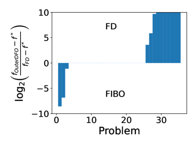
Figure B.1: Infeasible $x_{0}$. Log-ratio Plot for Comparing the Final Accuracy (3.1) of FIBO and FD.

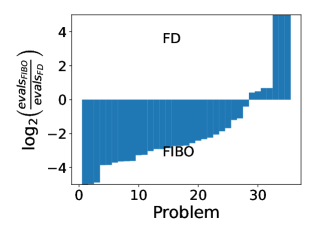
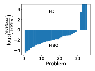
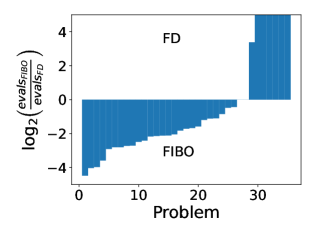
Figure B.2: Infeasible $x_{0}$. Log-ratio plot comparing FIBO and FD in terms of the number of function evaluations to satisfy (3.2) for $\tau=10^{-1}\text{ (upper left)},10^{-3}\text{ (upper right)},10^{-5}\text{ (bottom left)},10^{-7}\text{ (bottom right)}$.

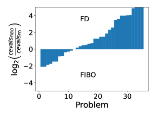
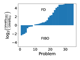
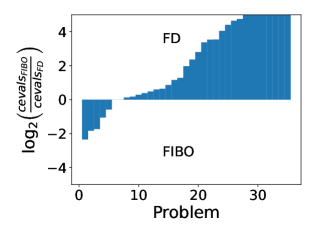
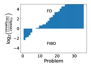
Figure B.3: Infeasible $x_{0}$. Log-ratio plot comparing FIBO and FD in terms of the number of constraint evaluations to satisfy (3.2) for $\tau=10^{-1}\text{ (upper left)},10^{-3}\text{ (upper right)},10^{-5}\text{ (bottom left)},10^{-7}\text{ (bottom right)}$.

As indicated by Figures B.1-B.3, the conclusions remain the same as in Section 3 and the cost of obtaining a feasible starting point is quite negligible.

			FIBO								knitro
Problem	n	m	#iter	#feval	time	$f$	feas err	#iter(sub)	#ceval	time(sub)	#iter	#feval	time	$f$	feas err
HS13	$2$	$1$	$3$	$5$	$0.32$	$1.000\text{\times}{10}^{00}$	$1.309\text{\times}{10}^{-14}$	136	193	0.28	$20$	$106$	$0.09$	$9.983\text{\times}{10}^{-01}$	$6.579\text{\times}{10}^{-10}$
HS22	$2$	$2$	$2$	$4$	$0.05$	$1.000\text{\times}{10}^{00}$	$0.000\text{\times}{10}^{00}$	10	27	0.03	$5$	$24$	$0.01$	$1.000\text{\times}{10}^{00}$	$0.000\text{\times}{10}^{00}$
HS23	$2$	$5$	$4$	$6$	$0.05$	$2.000\text{\times}{10}^{00}$	$0.000\text{\times}{10}^{00}$	12	18	0.03	$7$	$32$	$0.01$	$2.000\text{\times}{10}^{00}$	$0.000\text{\times}{10}^{00}$
HS26	$3$	$1$	$53$	$56$	$13.0$	$7.103\text{\times}{10}^{-10}$	$2.220\text{\times}{10}^{-16}$	5245	39138	12.85	$34$	$244$	$0.11$	$7.434\text{\times}{10}^{-12}$	$6.661\text{\times}{10}^{-16}$
HS32	$3$	$2$	$4$	$7$	$0.05$	$1.000\text{\times}{10}^{00}$	$0.000\text{\times}{10}^{00}$	10	17	0.03	$2$	$15$	$0.01$	$1.000\text{\times}{10}^{00}$	$0.000\text{\times}{10}^{00}$
HS34	$3$	$2$	$6$	$9$	$0.12$	$-8.340\text{\times}{10}^{-01}$	$1.776\text{\times}{10}^{-15}$	32	71	0.08	$7$	$44$	$0.02$	$-8.340\text{\times}{10}^{-01}$	$0.000\text{\times}{10}^{00}$
HS40	$4$	$3$	$22$	$26$	$0.37$	$-2.500\text{\times}{10}^{-01}$	$1.110\text{\times}{10}^{-16}$	56	229	0.26	$7$	$51$	$0.02$	$-2.500\text{\times}{10}^{-01}$	$1.665\text{\times}{10}^{-16}$
HS44	$4$	$6$	$3$	$8$	$0.06$	$-1.000\text{\times}{10}^{00}$(*)	$0.000\text{\times}{10}^{00}$	12	24	0.03	$5$	$36$	$0.01$	$-1.500\text{\times}{10}^{01}$	$0.000\text{\times}{10}^{00}$
HS47	$5$	$3$	$23$	$28$	$3.67$	$1.989\text{\times}{10}^{-07}$	$3.781\text{\times}{10}^{-11}$	1391	7879	3.47	$72$	$696$	$0.35$	$1.007\text{\times}{10}^{01}$	$6.661\text{\times}{10}^{-16}$
HS50	$5$	$3$	$19$	$24$	$1.18$	$1.056\text{\times}{10}^{00}$	$2.398\text{\times}{10}^{-14}$	126	424	1.1	$16$	$121$	$0.04$	$7.669\text{\times}{10}^{-17}$	$4.441\text{\times}{10}^{-16}$
HS64	$3$	$1$	$43$	$46$	$1.07$	$6.300\text{\times}{10}^{03}$	$0.000\text{\times}{10}^{00}$	300	674	0.95	$16$	$89$	$0.04$	$6.300\text{\times}{10}^{03}$	$1.110\text{\times}{10}^{-16}$
HS66	$3$	$2$	$2$	$6$	$0.04$	$5.182\text{\times}{10}^{-01}$(*)	$3.563\text{\times}{10}^{-12}$	7	13	0.02	$7$	$43$	$0.01$	$5.182\text{\times}{10}^{-01}$	$0.000\text{\times}{10}^{00}$
HS67	$3$	$14$	$45$	$49$	$1.71$	$-1.162\text{\times}{10}^{03}$(*)	$0.000\text{\times}{10}^{00}$	472	1409	1.59	$14$	$75$	$0.03$	$-1.162\text{\times}{10}^{03}$	$0.000\text{\times}{10}^{00}$
HS72	$4$	$2$	$7$	$11$	$0.32$	$7.277\text{\times}{10}^{02}$	$2.819\text{\times}{10}^{-18}$	44	111	0.21	$15$	$96$	$0.05$	$7.277\text{\times}{10}^{02}$	$1.301\text{\times}{10}^{-18}$
HS75	$4$	$5$	$16$	$20$	$0.54$	$5.174\text{\times}{10}^{03}$	$5.684\text{\times}{10}^{-14}$	97	185	0.43	$7$	$48$	$0.03$	$5.174\text{\times}{10}^{03}$	$2.842\text{\times}{10}^{-14}$
HS85	$5$	$21$	$31$	$36$	$1.47$	$-2.216\text{\times}{10}^{00}$	$0.000\text{\times}{10}^{00}$	357	904	1.31	$11$	$85$	$0.03$	$-2.216\text{\times}{10}^{00}$	$1.421\text{\times}{10}^{-14}$
HS87	$6$	$4$	$9$	$15$	$0.76$	$8.997\text{\times}{10}^{03}$	$2.274\text{\times}{10}^{-13}$	80	290	0.71	$14$	$216$	$0.07$	$8.997\text{\times}{10}^{03}$	$2.274\text{\times}{10}^{-13}$
HS88	$2$	$1$	$5$	$7$	$0.43$	$1.363\text{\times}{10}^{00}$	$0.000\text{\times}{10}^{00}$	92	329	0.39	$19$	$106$	$0.06$	$1.363\text{\times}{10}^{00}$	$0.000\text{\times}{10}^{00}$
HS89	$3$	$1$	$10$	$13$	$1.52$	$1.363\text{\times}{10}^{00}$	$0.000\text{\times}{10}^{00}$	246	1033	1.39	$28$	$172$	$0.09$	$1.363\text{\times}{10}^{00}$	$9.636\text{\times}{10}^{-18}$
HS90	$4$	$1$	$12$	$16$	$4.26$	$1.363\text{\times}{10}^{00}$	$0.000\text{\times}{10}^{00}$	738	3541	4.18	$48$	$426$	$0.24$	$1.363\text{\times}{10}^{00}$	$0.000\text{\times}{10}^{00}$
HS93	$6$	$2$	$42$	$48$	$2.9$	$1.351\text{\times}{10}^{02}$	$4.800\text{\times}{10}^{-12}$	517	2434	2.61	$26$	$295$	$0.08$	$1.351\text{\times}{10}^{02}$	$0.000\text{\times}{10}^{00}$
HS98	$6$	$4$	$3$	$10$	$0.09$	$3.136\text{\times}{10}^{00}$(*)	$1.776\text{\times}{10}^{-15}$	5	13	0.02	$6$	$56$	$0.01$	$3.136\text{\times}{10}^{00}$	$0.000\text{\times}{10}^{00}$
HS100	$7$	$4$	$106$	$113$	$29.47$	$6.806\text{\times}{10}^{02}$	$0.000\text{\times}{10}^{00}$	3280	22449	28.72	$51$	$587$	$0.16$	$6.806\text{\times}{10}^{02}$	$7.161\text{\times}{10}^{-15}$
HS101	$7$	$5$	$103$	$110$	$19.45$	$1.810\text{\times}{10}^{03}$	$3.955\text{\times}{10}^{-16}$	2616	15705	18.39	$56$	$582$	$0.22$	$1.810\text{\times}{10}^{03}$	$0.000\text{\times}{10}^{00}$
HS102	$7$	$5$	$103$	$110$	$15.14$	$9.119\text{\times}{10}^{02}$	$3.816\text{\times}{10}^{-16}$	1985	10248	13.86	$37$	$386$	$0.13$	$9.119\text{\times}{10}^{02}$	$2.498\text{\times}{10}^{-16}$
HS103	$7$	$5$	$56$	$63$	$5.53$	$5.437\text{\times}{10}^{02}$	$1.318\text{\times}{10}^{-16}$	825	4079	4.59	$28$	$284$	$0.08$	$5.437\text{\times}{10}^{02}$	$2.220\text{\times}{10}^{-16}$
HS104	$8$	$5$	$245$	$253$	$43.52$	$3.951\text{\times}{10}^{00}$	$9.714\text{\times}{10}^{-17}$	6813	37274	41.25	$17$	$190$	$0.04$	$3.951\text{\times}{10}^{00}$	$1.943\text{\times}{10}^{-16}$
LOADBAL	$31$	$31$	$1$	$15499$	$0.94$	$1.547\text{\times}{10}^{00}$(***)	$1.798\text{\times}{10}^{308}$	0	2	0.0	$40$	$1380$	$0.19$	$4.529\text{\times}{10}^{-01}$	$2.665\text{\times}{10}^{-15}$
OPTPRLOC	$30$	$30$	$9$	$39$	$1.01$	$-1.642\text{\times}{10}^{01}$	$1.990\text{\times}{10}^{-13}$	54	130	0.45	$12$	$456$	$0.06$	$-1.642\text{\times}{10}^{01}$	$1.279\text{\times}{10}^{-13}$
CB3	$3$	$3$	$1$	$4$	$0.03$	$2.000\text{\times}{10}^{00}$	$0.000\text{\times}{10}^{00}$	2	9	0.0	$7$	$40$	$0.01$	$2.000\text{\times}{10}^{00}$	$0.000\text{\times}{10}^{00}$
CRESC50	$6$	$100$	$1000$	$1006$	$215.05$	$5.939\text{\times}{10}^{-01}$(**)	$5.482\text{\times}{10}^{-13}$	26160	96697	210.07	$456$	$6023$	$2.46$	$5.948\text{\times}{10}^{-01}$	$4.547\text{\times}{10}^{-13}$
DEMBO7	$16$	$20$	$19$	$35$	$2.42$	$1.748\text{\times}{10}^{02}$	$4.073\text{\times}{10}^{-15}$	302	800	2.07	$45$	$893$	$0.2$	$1.748\text{\times}{10}^{02}$	$3.608\text{\times}{10}^{-16}$
DNIEPER	$57$	$24$	$24$	$81$	$7.75$	$1.874\text{\times}{10}^{04}$	$5.684\text{\times}{10}^{-14}$	273	1097	3.25	$6$	$418$	$0.07$	$1.874\text{\times}{10}^{04}$	$5.684\text{\times}{10}^{-14}$
EXPFITA	$5$	$22$	$1$	$10999$	$0.62$	$2.999\text{\times}{10}^{01}$(***)	$1.798\text{\times}{10}^{308}$	0	2	0.0	$19$	$140$	$0.05$	$1.137\text{\times}{10}^{-03}$	$1.421\text{\times}{10}^{-14}$
HIMMELBI	$100$	$12$	$114$	$215$	$72.25$	$-1.467\text{\times}{10}^{03}$(*)	$1.789\text{\times}{10}^{-09}$	2618	12588	67.95	$96$	$9950$	$1.01$	$-1.736\text{\times}{10}^{03}$	$2.842\text{\times}{10}^{-14}$
SYNTHES1	$6$	$6$	$1$	$2999$	$0.24$	$1.000\text{\times}{10}^{01}$(***)	$1.798\text{\times}{10}^{308}$	0	2	0.0	$9$	$81$	$0.02$	$7.593\text{\times}{10}^{-01}$	$1.110\text{\times}{10}^{-16}$
TWOBARS	$2$	$2$	$7$	$9$	$0.13$	$1.509\text{\times}{10}^{00}$	$0.000\text{\times}{10}^{00}$	24	113	0.09	$11$	$57$	$0.02$	$1.509\text{\times}{10}^{00}$	$2.220\text{\times}{10}^{-16}$
DIPIGRI	$7$	$4$	$116$	$123$	$85.87$	$6.806\text{\times}{10}^{02}$	$3.581\text{\times}{10}^{-11}$	7461	26265	84.59	$48$	$581$	$0.16$	$6.806\text{\times}{10}^{02}$	$0.000\text{\times}{10}^{00}$

Table B.1: Noiseless Problems with Infeasible $x_{0}$; $n$: number of variables, $m$: number of constraints, #iter: number of (outer) iterations, #feval: number of function evaluations, time: total CPU time passed, $f$: final objective value, feas err: final feasibility error, #iter(sub): total number of iterations for solving TR subproblem, #ceval: total number of constraint evaluations(note that the number of constraint evaluations and function evaluations are same for KNITRO), time(sub): total CPU time elapsed for solving subproblem. * indicates that FIBO terminates with singular interpolation system error, ** indicates that FIBO terminates with maximum number of iterations, *** indicates that FIBO terminates with maximum number of function evaluations.

			FIBO								knitro
Problem	n	m	#iter	#feval	time	$f$	feas err	#iter(sub)	#ceval	time(sub)	#iter	#feval	time	$f$	feas err
HS13	$2$	$1$	$2$	$4$	$0.2$	$1.000\text{\times}{10}^{00}$	$1.310\text{\times}{10}^{-14}$	75	106	0.19	$8$	$38$	$0.02$	$1.080\text{\times}{10}^{00}$	$0.000\text{\times}{10}^{00}$
HS22	$2$	$2$	$1$	$3$	$0.04$	$1.000\text{\times}{10}^{00}$	$1.789\text{\times}{10}^{-12}$	9	25	0.02	$3$	$16$	$0.01$	$1.000\text{\times}{10}^{00}$	$1.231\text{\times}{10}^{-06}$
HS23	$2$	$5$	$3$	$5$	$0.07$	$2.000\text{\times}{10}^{00}$	$0.000\text{\times}{10}^{00}$	11	16	0.03	$3$	$16$	$0.01$	$2.075\text{\times}{10}^{00}$	$0.000\text{\times}{10}^{00}$
HS26	$3$	$1$	$4$	$7$	$0.09$	$1.996\text{\times}{10}^{-02}$	$9.592\text{\times}{10}^{-14}$	32	67	0.07	$14$	$87$	$0.03$	$4.252\text{\times}{10}^{-07}$	$9.633\text{\times}{10}^{-07}$
HS32	$3$	$2$	$4$	$7$	$0.1$	$1.000\text{\times}{10}^{00}$	$0.000\text{\times}{10}^{00}$	10	17	0.04	$2$	$15$	$0.01$	$1.000\text{\times}{10}^{00}$	$0.000\text{\times}{10}^{00}$
HS34	$3$	$2$	$5$	$8$	$0.11$	$-7.820\text{\times}{10}^{-01}$	$1.066\text{\times}{10}^{-14}$	31	69	0.08	$4$	$29$	$0.01$	$-8.266\text{\times}{10}^{-01}$	$0.000\text{\times}{10}^{00}$
HS40	$4$	$3$	$1$	$5$	$0.03$	$-2.454\text{\times}{10}^{-01}$	$2.554\text{\times}{10}^{-15}$	5	19	0.01	$4$	$33$	$0.01$	$-2.500\text{\times}{10}^{-01}$	$5.162\text{\times}{10}^{-08}$
HS44	$4$	$6$	$3$	$8$	$0.1$	$-1.000\text{\times}{10}^{00}$(*)	$0.000\text{\times}{10}^{00}$	12	24	0.07	$4$	$30$	$0.01$	$-1.500\text{\times}{10}^{01}$	$0.000\text{\times}{10}^{00}$
HS47	$5$	$3$	$6$	$11$	$0.15$	$5.639\text{\times}{10}^{-02}$	$1.466\text{\times}{10}^{-12}$	46	119	0.12	$17$	$134$	$0.04$	$4.638\text{\times}{10}^{-08}$	$3.167\text{\times}{10}^{-09}$
HS50	$5$	$3$	$19$	$24$	$1.26$	$1.056\text{\times}{10}^{00}$	$2.398\text{\times}{10}^{-14}$	126	423	1.19	$9$	$71$	$0.03$	$4.941\text{\times}{10}^{-02}$	$4.441\text{\times}{10}^{-16}$
HS64	$3$	$1$	$1$	$4$	$0.09$	$6.813\text{\times}{10}^{03}$	$4.742\text{\times}{10}^{-11}$	14	84	0.05	$5$	$30$	$0.02$	$6.705\text{\times}{10}^{03}$	$3.942\text{\times}{10}^{-05}$
HS66	$3$	$2$	$1$	$4$	$0.05$	$5.800\text{\times}{10}^{-01}$	$3.563\text{\times}{10}^{-12}$	6	11	0.01	$0$	$3$	$0.0$	$5.800\text{\times}{10}^{-01}$	$0.000\text{\times}{10}^{00}$
HS67	$3$	$14$	$31$	$34$	$1.92$	$-1.053\text{\times}{10}^{03}$	$0.000\text{\times}{10}^{00}$	402	1320	1.82	$8$	$45$	$0.02$	$-1.157\text{\times}{10}^{03}$	$0.000\text{\times}{10}^{00}$
HS72	$4$	$2$	$1$	$5$	$0.03$	$7.407\text{\times}{10}^{02}$	$0.000\text{\times}{10}^{00}$	2	17	0.01	$11$	$72$	$0.04$	$7.277\text{\times}{10}^{02}$	$8.766\text{\times}{10}^{-07}$
HS75	$4$	$5$	$1$	$5$	$0.06$	$5.350\text{\times}{10}^{03}$	$1.259\text{\times}{10}^{-08}$	4	13	0.01	$5$	$36$	$0.03$	$5.174\text{\times}{10}^{03}$	$1.880\text{\times}{10}^{-04}$
HS85	$5$	$21$	$29$	$34$	$1.23$	$-2.061\text{\times}{10}^{00}$	$1.421\text{\times}{10}^{-14}$	348	881	1.04	$10$	$78$	$0.03$	$-2.216\text{\times}{10}^{00}$	$2.389\text{\times}{10}^{-08}$
HS87	$6$	$4$	$1$	$7$	$0.1$	$8.997\text{\times}{10}^{03}$	$2.274\text{\times}{10}^{-13}$	9	27	0.06	$3$	$33$	$0.02$	$8.997\text{\times}{10}^{03}$	$3.775\text{\times}{10}^{-08}$
HS88	$2$	$1$	$1$	$3$	$0.13$	$1.385\text{\times}{10}^{00}$	$2.158\text{\times}{10}^{-14}$	19	52	0.07	$16$	$94$	$0.05$	$1.363\text{\times}{10}^{00}$	$1.074\text{\times}{10}^{-08}$
HS89	$3$	$1$	$2$	$5$	$0.41$	$1.365\text{\times}{10}^{00}$	$1.123\text{\times}{10}^{-16}$	57	349	0.28	$23$	$147$	$0.07$	$1.362\text{\times}{10}^{00}$	$7.400\text{\times}{10}^{-07}$
HS90	$4$	$1$	$2$	$6$	$0.56$	$1.446\text{\times}{10}^{00}$	$6.661\text{\times}{10}^{-16}$	86	464	0.52	$36$	$334$	$0.15$	$1.363\text{\times}{10}^{00}$	$1.142\text{\times}{10}^{-07}$
HS93	$6$	$2$	$1$	$7$	$0.13$	$1.371\text{\times}{10}^{02}$	$2.946\text{\times}{10}^{-11}$	10	25	0.11	$0$	$5$	$0.0$	$1.371\text{\times}{10}^{02}$	$0.000\text{\times}{10}^{00}$
HS98	$6$	$4$	$2$	$8$	$0.06$	$3.136\text{\times}{10}^{00}$	$0.000\text{\times}{10}^{00}$	4	11	0.02	$4$	$40$	$0.01$	$3.214\text{\times}{10}^{00}$	$0.000\text{\times}{10}^{00}$
HS100	$7$	$4$	$1$	$8$	$0.14$	$7.140\text{\times}{10}^{02}$	$0.000\text{\times}{10}^{00}$	22	80	0.12	$0$	$5$	$0.0$	$7.140\text{\times}{10}^{02}$	$0.000\text{\times}{10}^{00}$
HS101	$7$	$5$	$26$	$33$	$5.28$	$1.982\text{\times}{10}^{03}$	$3.053\text{\times}{10}^{-16}$	740	4391	5.04	$26$	$269$	$0.1$	$1.810\text{\times}{10}^{03}$	$2.249\text{\times}{10}^{-05}$
HS102	$7$	$5$	$34$	$41$	$4.59$	$9.948\text{\times}{10}^{02}$	$2.776\text{\times}{10}^{-17}$	641	3328	4.29	$25$	$272$	$0.09$	$9.129\text{\times}{10}^{02}$	$5.866\text{\times}{10}^{-05}$
HS103	$7$	$5$	$15$	$22$	$1.72$	$5.623\text{\times}{10}^{02}$	$8.913\text{\times}{10}^{-12}$	276	1270	1.63	$20$	$212$	$0.07$	$5.434\text{\times}{10}^{02}$	$3.104\text{\times}{10}^{-04}$
HS104	$8$	$5$	$1$	$9$	$0.15$	$4.200\text{\times}{10}^{00}$	$1.459\text{\times}{10}^{-11}$	14	47	0.11	$11$	$130$	$0.03$	$3.951\text{\times}{10}^{00}$	$5.769\text{\times}{10}^{-07}$
LOADBAL	$31$	$31$	$1$	$15499$	$0.99$	$1.547\text{\times}{10}^{00}$(***)	$1.798\text{\times}{10}^{308}$	0	2	0.0	$6$	$231$	$0.04$	$5.252\text{\times}{10}^{-01}$	$1.710\text{\times}{10}^{-14}$
OPTPRLOC	$30$	$30$	$5$	$35$	$0.48$	$-1.567\text{\times}{10}^{01}$	$2.220\text{\times}{10}^{-16}$	44	107	0.4	$12$	$456$	$0.06$	$-1.642\text{\times}{10}^{01}$	$1.279\text{\times}{10}^{-13}$
CB3	$3$	$3$	$1$	$4$	$0.02$	$2.000\text{\times}{10}^{00}$	$0.000\text{\times}{10}^{00}$	2	9	0.01	$5$	$30$	$0.01$	$2.000\text{\times}{10}^{00}$	$3.017\text{\times}{10}^{-06}$
CRESC50	$6$	$100$	$16$	$22$	$2.49$	$6.057\text{\times}{10}^{-01}$	$9.032\text{\times}{10}^{-11}$	344	1534	2.38	$10$	$91$	$0.06$	$6.567\text{\times}{10}^{-01}$	$9.586\text{\times}{10}^{-04}$
DEMBO7	$16$	$20$	$13$	$29$	$1.44$	$1.879\text{\times}{10}^{02}$	$5.917\text{\times}{10}^{-08}$	198	512	1.19	$16$	$358$	$0.12$	$1.748\text{\times}{10}^{02}$	$1.074\text{\times}{10}^{-05}$
DNIEPER	$57$	$24$	$4$	$61$	$1.86$	$1.941\text{\times}{10}^{04}$	$4.264\text{\times}{10}^{-11}$	96	460	1.35	$5$	$359$	$0.07$	$1.874\text{\times}{10}^{04}$	$3.740\text{\times}{10}^{-10}$
EXPFITA	$5$	$22$	$1$	$10999$	$0.62$	$2.999\text{\times}{10}^{01}$(***)	$1.798\text{\times}{10}^{308}$	0	2	0.0	$7$	$56$	$0.02$	$9.889\text{\times}{10}^{-02}$	$1.354\text{\times}{10}^{-14}$
HIMMELBI	$100$	$12$	$114$	$215$	$70.51$	$-1.467\text{\times}{10}^{03}$(*)	$1.789\text{\times}{10}^{-09}$	2618	12588	68.05	$3$	$408$	$0.05$	$-1.625\text{\times}{10}^{03}$	$0.000\text{\times}{10}^{00}$
SYNTHES1	$6$	$6$	$1$	$2999$	$0.23$	$1.000\text{\times}{10}^{01}$(***)	$1.798\text{\times}{10}^{308}$	0	2	0.0	$7$	$65$	$0.02$	$7.593\text{\times}{10}^{-01}$	$3.261\text{\times}{10}^{-07}$
TWOBARS	$2$	$2$	$2$	$4$	$0.07$	$1.523\text{\times}{10}^{00}$	$7.885\text{\times}{10}^{-09}$	13	43	0.04	$4$	$26$	$0.01$	$1.558\text{\times}{10}^{00}$	$0.000\text{\times}{10}^{00}$
DIPIGRI	$7$	$4$	$1$	$8$	$0.15$	$7.140\text{\times}{10}^{02}$	$0.000\text{\times}{10}^{00}$	22	80	0.13	$0$	$5$	$0.0$	$7.140\text{\times}{10}^{02}$	$0.000\text{\times}{10}^{00}$

Table B.2: Noiseless Problems with Infeasible $x_{0}$. $\tau=10^{-1}$; $n$: number of variables, $m$: number of constraints, #iter: number of (outer) iterations, #feval: number of function evaluations, time: total CPU time passed, $f$: final objective value, feas err: final feasibility error, #iter(sub): total number of iterations for solving TR subproblem, #ceval: total number of constraint evaluations(note that the number of constraint evaluations and function evaluations are same for KNITRO), time(sub): total CPU time elapsed for solving subproblem. * indicates that FIBO terminates with singular interpolation system error, ** indicates that FIBO terminates with maximum number of iterations, *** indicates that FIBO terminates with maximum number of function evaluations.

			FIBO								knitro
Problem	n	m	#iter	#feval	time	$f$	feas err	#iter(sub)	#ceval	time(sub)	#iter	#feval	time	$f$	feas err
HS13	$2$	$1$	$2$	$4$	$0.19$	$1.000\text{\times}{10}^{00}$	$1.310\text{\times}{10}^{-14}$	75	106	0.17	$18$	$90$	$0.08$	$1.001\text{\times}{10}^{00}$	$0.000\text{\times}{10}^{00}$
HS22	$2$	$2$	$1$	$3$	$0.04$	$1.000\text{\times}{10}^{00}$	$1.789\text{\times}{10}^{-12}$	9	25	0.02	$3$	$16$	$0.01$	$1.000\text{\times}{10}^{00}$	$1.231\text{\times}{10}^{-06}$
HS23	$2$	$5$	$3$	$5$	$0.05$	$2.000\text{\times}{10}^{00}$	$0.000\text{\times}{10}^{00}$	11	16	0.03	$4$	$20$	$0.01$	$2.001\text{\times}{10}^{00}$	$0.000\text{\times}{10}^{00}$
HS26	$3$	$1$	$36$	$39$	$1.86$	$1.737\text{\times}{10}^{-04}$	$1.040\text{\times}{10}^{-12}$	754	4339	1.77	$14$	$87$	$0.03$	$4.252\text{\times}{10}^{-07}$	$9.633\text{\times}{10}^{-07}$
HS32	$3$	$2$	$4$	$7$	$0.06$	$1.000\text{\times}{10}^{00}$	$0.000\text{\times}{10}^{00}$	10	17	0.03	$2$	$15$	$0.01$	$1.000\text{\times}{10}^{00}$	$0.000\text{\times}{10}^{00}$
HS34	$3$	$2$	$6$	$9$	$0.11$	$-8.340\text{\times}{10}^{-01}$	$1.776\text{\times}{10}^{-15}$	32	71	0.08	$6$	$39$	$0.01$	$-8.340\text{\times}{10}^{-01}$	$5.446\text{\times}{10}^{-09}$
HS40	$4$	$3$	$2$	$6$	$0.05$	$-2.491\text{\times}{10}^{-01}$	$2.189\text{\times}{10}^{-09}$	8	25	0.02	$4$	$33$	$0.01$	$-2.500\text{\times}{10}^{-01}$	$5.162\text{\times}{10}^{-08}$
HS44	$4$	$6$	$3$	$8$	$0.05$	$-1.000\text{\times}{10}^{00}$(*)	$0.000\text{\times}{10}^{00}$	12	24	0.03	$4$	$30$	$0.01$	$-1.500\text{\times}{10}^{01}$	$0.000\text{\times}{10}^{00}$
HS47	$5$	$3$	$23$	$28$	$3.41$	$1.989\text{\times}{10}^{-07}$	$3.781\text{\times}{10}^{-11}$	1391	7878	3.33	$72$	$696$	$0.36$	$1.007\text{\times}{10}^{01}$	$6.661\text{\times}{10}^{-16}$
HS50	$5$	$3$	$19$	$24$	$1.02$	$1.056\text{\times}{10}^{00}$	$2.398\text{\times}{10}^{-14}$	126	423	0.96	$11$	$85$	$0.03$	$1.339\text{\times}{10}^{-06}$	$8.882\text{\times}{10}^{-16}$
HS64	$3$	$1$	$13$	$16$	$0.5$	$6.303\text{\times}{10}^{03}$	$1.443\text{\times}{10}^{-15}$	126	411	0.44	$9$	$54$	$0.02$	$6.306\text{\times}{10}^{03}$	$0.000\text{\times}{10}^{00}$
HS66	$3$	$2$	$2$	$5$	$0.03$	$5.182\text{\times}{10}^{-01}$	$3.563\text{\times}{10}^{-12}$	7	13	0.02	$3$	$21$	$0.01$	$5.186\text{\times}{10}^{-01}$	$0.000\text{\times}{10}^{00}$
HS67	$3$	$14$	$38$	$41$	$1.51$	$-1.162\text{\times}{10}^{03}$	$0.000\text{\times}{10}^{00}$	448	1378	1.42	$9$	$50$	$0.02$	$-1.161\text{\times}{10}^{03}$	$0.000\text{\times}{10}^{00}$
HS72	$4$	$2$	$5$	$9$	$0.2$	$7.284\text{\times}{10}^{02}$	$0.000\text{\times}{10}^{00}$	38	102	0.16	$11$	$72$	$0.05$	$7.277\text{\times}{10}^{02}$	$8.766\text{\times}{10}^{-07}$
HS75	$4$	$5$	$16$	$20$	$0.35$	$5.174\text{\times}{10}^{03}$	$5.684\text{\times}{10}^{-14}$	97	185	0.28	$5$	$36$	$0.03$	$5.174\text{\times}{10}^{03}$	$1.880\text{\times}{10}^{-04}$
HS85	$5$	$21$	$31$	$36$	$0.96$	$-2.216\text{\times}{10}^{00}$	$0.000\text{\times}{10}^{00}$	357	904	0.87	$10$	$78$	$0.03$	$-2.216\text{\times}{10}^{00}$	$2.389\text{\times}{10}^{-08}$
HS87	$6$	$4$	$1$	$7$	$0.09$	$8.997\text{\times}{10}^{03}$	$2.274\text{\times}{10}^{-13}$	9	27	0.06	$3$	$33$	$0.01$	$8.997\text{\times}{10}^{03}$	$3.775\text{\times}{10}^{-08}$
HS88	$2$	$1$	$2$	$4$	$0.23$	$1.363\text{\times}{10}^{00}$	$9.216\text{\times}{10}^{-16}$	41	150	0.19	$16$	$94$	$0.05$	$1.363\text{\times}{10}^{00}$	$1.074\text{\times}{10}^{-08}$
HS89	$3$	$1$	$4$	$7$	$0.6$	$1.363\text{\times}{10}^{00}$	$3.663\text{\times}{10}^{-16}$	101	518	0.48	$23$	$147$	$0.07$	$1.362\text{\times}{10}^{00}$	$7.400\text{\times}{10}^{-07}$
HS90	$4$	$1$	$6$	$10$	$1.57$	$1.363\text{\times}{10}^{00}$	$5.260\text{\times}{10}^{-17}$	277	1551	1.52	$36$	$334$	$0.16$	$1.363\text{\times}{10}^{00}$	$1.142\text{\times}{10}^{-07}$
HS93	$6$	$2$	$21$	$27$	$1.51$	$1.352\text{\times}{10}^{02}$	$4.695\text{\times}{10}^{-11}$	333	1707	1.43	$8$	$87$	$0.03$	$1.351\text{\times}{10}^{02}$	$0.000\text{\times}{10}^{00}$
HS98	$6$	$4$	$2$	$8$	$0.06$	$3.136\text{\times}{10}^{00}$	$0.000\text{\times}{10}^{00}$	4	11	0.01	$6$	$56$	$0.01$	$3.136\text{\times}{10}^{00}$	$0.000\text{\times}{10}^{00}$
HS100	$7$	$4$	$51$	$58$	$15.19$	$6.813\text{\times}{10}^{02}$	$1.388\text{\times}{10}^{-17}$	1609	11183	15.01	$3$	$55$	$0.02$	$6.811\text{\times}{10}^{02}$	$0.000\text{\times}{10}^{00}$
HS101	$7$	$5$	$44$	$51$	$7.84$	$1.812\text{\times}{10}^{03}$	$3.006\text{\times}{10}^{-10}$	1239	7252	7.65	$26$	$269$	$0.1$	$1.810\text{\times}{10}^{03}$	$2.249\text{\times}{10}^{-05}$
HS102	$7$	$5$	$69$	$76$	$10.15$	$9.125\text{\times}{10}^{02}$	$4.272\text{\times}{10}^{-13}$	1483	7671	9.89	$26$	$282$	$0.09$	$9.120\text{\times}{10}^{02}$	$3.705\text{\times}{10}^{-06}$
HS103	$7$	$5$	$37$	$44$	$3.97$	$5.437\text{\times}{10}^{02}$	$7.980\text{\times}{10}^{-16}$	671	3472	3.8	$20$	$212$	$0.07$	$5.434\text{\times}{10}^{02}$	$3.104\text{\times}{10}^{-04}$
HS104	$8$	$5$	$47$	$55$	$6.2$	$3.952\text{\times}{10}^{00}$	$5.218\text{\times}{10}^{-15}$	1210	6053	5.99	$11$	$130$	$0.03$	$3.951\text{\times}{10}^{00}$	$5.769\text{\times}{10}^{-07}$
LOADBAL	$31$	$31$	$1$	$15499$	$0.92$	$1.547\text{\times}{10}^{00}$(***)	$1.798\text{\times}{10}^{308}$	0	2	0.0	$9$	$330$	$0.05$	$4.531\text{\times}{10}^{-01}$	$1.421\text{\times}{10}^{-14}$
OPTPRLOC	$30$	$30$	$6$	$36$	$0.45$	$-1.642\text{\times}{10}^{01}$	$0.000\text{\times}{10}^{00}$	47	114	0.39	$12$	$456$	$0.06$	$-1.642\text{\times}{10}^{01}$	$1.279\text{\times}{10}^{-13}$
CB3	$3$	$3$	$1$	$4$	$0.03$	$2.000\text{\times}{10}^{00}$	$0.000\text{\times}{10}^{00}$	2	9	0.01	$5$	$30$	$0.01$	$2.000\text{\times}{10}^{00}$	$3.017\text{\times}{10}^{-06}$
CRESC50	$6$	$100$	$68$	$74$	$18.03$	$5.942\text{\times}{10}^{-01}$	$0.000\text{\times}{10}^{00}$	2416	11263	17.76	$456$	$6023$	$2.47$	$5.948\text{\times}{10}^{-01}$	$4.547\text{\times}{10}^{-13}$
DEMBO7	$16$	$20$	$18$	$34$	$2.17$	$1.749\text{\times}{10}^{02}$	$1.067\text{\times}{10}^{-10}$	301	798	2.03	$16$	$358$	$0.11$	$1.748\text{\times}{10}^{02}$	$1.074\text{\times}{10}^{-05}$
DNIEPER	$57$	$24$	$5$	$62$	$1.45$	$1.874\text{\times}{10}^{04}$	$1.405\text{\times}{10}^{-09}$	100	468	1.35	$5$	$359$	$0.07$	$1.874\text{\times}{10}^{04}$	$3.740\text{\times}{10}^{-10}$
EXPFITA	$5$	$22$	$1$	$10999$	$0.59$	$2.999\text{\times}{10}^{01}$(***)	$1.798\text{\times}{10}^{308}$	0	2	0.0	$12$	$91$	$0.03$	$1.355\text{\times}{10}^{-03}$	$6.750\text{\times}{10}^{-14}$
HIMMELBI	$100$	$12$	$114$	$215$	$68.61$	$-1.467\text{\times}{10}^{03}$(*)	$1.789\text{\times}{10}^{-09}$	2618	12588	67.1	$16$	$1734$	$0.19$	$-1.734\text{\times}{10}^{03}$	$3.553\text{\times}{10}^{-15}$
SYNTHES1	$6$	$6$	$1$	$2999$	$0.22$	$1.000\text{\times}{10}^{01}$(***)	$1.798\text{\times}{10}^{308}$	0	2	0.0	$7$	$65$	$0.02$	$7.593\text{\times}{10}^{-01}$	$3.261\text{\times}{10}^{-07}$
TWOBARS	$2$	$2$	$3$	$5$	$0.08$	$1.509\text{\times}{10}^{00}$	$4.742\text{\times}{10}^{-11}$	16	60	0.05	$9$	$49$	$0.02$	$1.509\text{\times}{10}^{00}$	$8.844\text{\times}{10}^{-08}$
DIPIGRI	$7$	$4$	$51$	$58$	$11.34$	$6.812\text{\times}{10}^{02}$	$6.939\text{\times}{10}^{-18}$	1491	9510	11.16	$3$	$55$	$0.01$	$6.811\text{\times}{10}^{02}$	$0.000\text{\times}{10}^{00}$

Table B.3: Noiseless Problems with Infeasible $x_{0}$. $\tau=10^{-3}$; $n$: number of variables, $m$: number of constraints, #iter: number of (outer) iterations, #feval: number of function evaluations, time: total CPU time passed, $f$: final objective value, feas err: final feasibility error, #iter(sub): total number of iterations for solving TR subproblem, #ceval: total number of constraint evaluations(note that the number of constraint evaluations and function evaluations are same for KNITRO), time(sub): total CPU time elapsed for solving subproblem. * indicates that FIBO terminates with singular interpolation system error, ** indicates that FIBO terminates with maximum number of iterations, *** indicates that FIBO terminates with maximum number of function evaluations.

			FIBO								knitro
Problem	n	m	#iter	#feval	time	$f$	feas err	#iter(sub)	#ceval	time(sub)	#iter	#feval	time	$f$	feas err
HS13	$2$	$1$	$3$	$5$	$0.29$	$1.000\text{\times}{10}^{00}$	$1.309\text{\times}{10}^{-14}$	136	191	0.28	$19$	$102$	$0.09$	$9.983\text{\times}{10}^{-01}$	$6.579\text{\times}{10}^{-10}$
HS22	$2$	$2$	$1$	$3$	$0.04$	$1.000\text{\times}{10}^{00}$	$1.789\text{\times}{10}^{-12}$	9	25	0.02	$3$	$16$	$0.01$	$1.000\text{\times}{10}^{00}$	$1.231\text{\times}{10}^{-06}$
HS23	$2$	$5$	$3$	$5$	$0.04$	$2.000\text{\times}{10}^{00}$	$0.000\text{\times}{10}^{00}$	11	16	0.02	$5$	$24$	$0.01$	$2.000\text{\times}{10}^{00}$	$0.000\text{\times}{10}^{00}$
HS26	$3$	$1$	$38$	$41$	$8.15$	$8.872\text{\times}{10}^{-07}$	$4.441\text{\times}{10}^{-16}$	3356	26977	8.07	$14$	$87$	$0.03$	$4.252\text{\times}{10}^{-07}$	$9.633\text{\times}{10}^{-07}$
HS32	$3$	$2$	$4$	$7$	$0.05$	$1.000\text{\times}{10}^{00}$	$0.000\text{\times}{10}^{00}$	10	17	0.03	$2$	$15$	$0.01$	$1.000\text{\times}{10}^{00}$	$0.000\text{\times}{10}^{00}$
HS34	$3$	$2$	$6$	$9$	$0.11$	$-8.340\text{\times}{10}^{-01}$	$1.776\text{\times}{10}^{-15}$	32	71	0.08	$6$	$39$	$0.01$	$-8.340\text{\times}{10}^{-01}$	$5.446\text{\times}{10}^{-09}$
HS40	$4$	$3$	$4$	$8$	$0.08$	$-2.500\text{\times}{10}^{-01}$	$1.058\text{\times}{10}^{-12}$	13	36	0.04	$4$	$33$	$0.01$	$-2.500\text{\times}{10}^{-01}$	$5.162\text{\times}{10}^{-08}$
HS44	$4$	$6$	$3$	$8$	$0.05$	$-1.000\text{\times}{10}^{00}$(*)	$0.000\text{\times}{10}^{00}$	12	24	0.04	$4$	$30$	$0.01$	$-1.500\text{\times}{10}^{01}$	$0.000\text{\times}{10}^{00}$
HS47	$5$	$3$	$23$	$28$	$3.42$	$1.989\text{\times}{10}^{-07}$	$3.781\text{\times}{10}^{-11}$	1391	7878	3.35	$72$	$696$	$0.36$	$1.007\text{\times}{10}^{01}$	$6.661\text{\times}{10}^{-16}$
HS50	$5$	$3$	$19$	$24$	$1.11$	$1.056\text{\times}{10}^{00}$	$2.398\text{\times}{10}^{-14}$	126	423	1.06	$11$	$85$	$0.03$	$1.339\text{\times}{10}^{-06}$	$8.882\text{\times}{10}^{-16}$
HS64	$3$	$1$	$17$	$20$	$0.58$	$6.300\text{\times}{10}^{03}$	$0.000\text{\times}{10}^{00}$	156	447	0.52	$11$	$64$	$0.03$	$6.300\text{\times}{10}^{03}$	$6.916\text{\times}{10}^{-06}$
HS66	$3$	$2$	$2$	$5$	$0.03$	$5.182\text{\times}{10}^{-01}$	$3.563\text{\times}{10}^{-12}$	7	13	0.02	$4$	$27$	$0.01$	$5.182\text{\times}{10}^{-01}$	$0.000\text{\times}{10}^{00}$
HS67	$3$	$14$	$39$	$42$	$1.46$	$-1.162\text{\times}{10}^{03}$	$0.000\text{\times}{10}^{00}$	450	1381	1.38	$10$	$55$	$0.03$	$-1.162\text{\times}{10}^{03}$	$0.000\text{\times}{10}^{00}$
HS72	$4$	$2$	$6$	$10$	$0.27$	$7.277\text{\times}{10}^{02}$	$6.263\text{\times}{10}^{-14}$	43	109	0.22	$11$	$72$	$0.04$	$7.277\text{\times}{10}^{02}$	$8.766\text{\times}{10}^{-07}$
HS75	$4$	$5$	$16$	$20$	$0.34$	$5.174\text{\times}{10}^{03}$	$5.684\text{\times}{10}^{-14}$	97	185	0.27	$5$	$36$	$0.03$	$5.174\text{\times}{10}^{03}$	$1.880\text{\times}{10}^{-04}$
HS85	$5$	$21$	$31$	$36$	$0.94$	$-2.216\text{\times}{10}^{00}$	$0.000\text{\times}{10}^{00}$	357	904	0.83	$10$	$78$	$0.03$	$-2.216\text{\times}{10}^{00}$	$2.389\text{\times}{10}^{-08}$
HS87	$6$	$4$	$2$	$8$	$0.13$	$8.997\text{\times}{10}^{03}$	$7.844\text{\times}{10}^{-12}$	15	46	0.1	$3$	$33$	$0.02$	$8.997\text{\times}{10}^{03}$	$3.775\text{\times}{10}^{-08}$
HS88	$2$	$1$	$4$	$6$	$0.34$	$1.363\text{\times}{10}^{00}$	$1.301\text{\times}{10}^{-14}$	69	229	0.3	$16$	$94$	$0.05$	$1.363\text{\times}{10}^{00}$	$1.074\text{\times}{10}^{-08}$
HS89	$3$	$1$	$5$	$8$	$0.64$	$1.363\text{\times}{10}^{00}$	$0.000\text{\times}{10}^{00}$	113	576	0.54	$23$	$147$	$0.08$	$1.362\text{\times}{10}^{00}$	$7.400\text{\times}{10}^{-07}$
HS90	$4$	$1$	$11$	$15$	$3.63$	$1.363\text{\times}{10}^{00}$	$8.118\text{\times}{10}^{-18}$	718	3460	3.57	$36$	$334$	$0.18$	$1.363\text{\times}{10}^{00}$	$1.142\text{\times}{10}^{-07}$
HS93	$6$	$2$	$25$	$31$	$1.58$	$1.351\text{\times}{10}^{02}$	$3.331\text{\times}{10}^{-16}$	371	1843	1.5	$8$	$87$	$0.03$	$1.351\text{\times}{10}^{02}$	$0.000\text{\times}{10}^{00}$
HS98	$6$	$4$	$2$	$8$	$0.05$	$3.136\text{\times}{10}^{00}$	$0.000\text{\times}{10}^{00}$	4	11	0.02	$6$	$56$	$0.01$	$3.136\text{\times}{10}^{00}$	$0.000\text{\times}{10}^{00}$
HS100	$7$	$4$	$89$	$96$	$24.87$	$6.806\text{\times}{10}^{02}$	$0.000\text{\times}{10}^{00}$	2860	19400	24.54	$14$	$212$	$0.07$	$6.806\text{\times}{10}^{02}$	$0.000\text{\times}{10}^{00}$
HS101	$7$	$5$	$71$	$78$	$12.77$	$1.810\text{\times}{10}^{03}$	$2.776\text{\times}{10}^{-16}$	2004	11927	12.48	$27$	$280$	$0.1$	$1.810\text{\times}{10}^{03}$	$2.398\text{\times}{10}^{-05}$
HS102	$7$	$5$	$78$	$85$	$10.48$	$9.119\text{\times}{10}^{02}$	$0.000\text{\times}{10}^{00}$	1601	8233	10.11	$28$	$305$	$0.09$	$9.119\text{\times}{10}^{02}$	$2.176\text{\times}{10}^{-06}$
HS103	$7$	$5$	$39$	$46$	$4.26$	$5.437\text{\times}{10}^{02}$	$6.106\text{\times}{10}^{-16}$	685	3522	4.09	$20$	$212$	$0.07$	$5.434\text{\times}{10}^{02}$	$3.104\text{\times}{10}^{-04}$
HS104	$8$	$5$	$80$	$88$	$13.33$	$3.951\text{\times}{10}^{00}$	$0.000\text{\times}{10}^{00}$	2262	12387	13.0	$11$	$130$	$0.03$	$3.951\text{\times}{10}^{00}$	$5.769\text{\times}{10}^{-07}$
LOADBAL	$31$	$31$	$1$	$15499$	$0.89$	$1.547\text{\times}{10}^{00}$(***)	$1.798\text{\times}{10}^{308}$	0	2	0.0	$17$	$594$	$0.09$	$4.529\text{\times}{10}^{-01}$	$1.483\text{\times}{10}^{-14}$
OPTPRLOC	$30$	$30$	$8$	$38$	$0.54$	$-1.642\text{\times}{10}^{01}$	$4.504\text{\times}{10}^{-10}$	53	128	0.44	$12$	$456$	$0.06$	$-1.642\text{\times}{10}^{01}$	$1.279\text{\times}{10}^{-13}$
CB3	$3$	$3$	$1$	$4$	$0.03$	$2.000\text{\times}{10}^{00}$	$0.000\text{\times}{10}^{00}$	2	9	0.01	$5$	$30$	$0.01$	$2.000\text{\times}{10}^{00}$	$3.017\text{\times}{10}^{-06}$
CRESC50	$6$	$100$	$1000$	$1006$	$214.67$	$5.939\text{\times}{10}^{-01}$(**)	$5.482\text{\times}{10}^{-13}$	26160	96697	211.17	$456$	$6023$	$2.37$	$5.948\text{\times}{10}^{-01}$	$4.547\text{\times}{10}^{-13}$
DEMBO7	$16$	$20$	$19$	$35$	$2.11$	$1.748\text{\times}{10}^{02}$	$4.073\text{\times}{10}^{-15}$	302	800	1.97	$16$	$358$	$0.1$	$1.748\text{\times}{10}^{02}$	$1.074\text{\times}{10}^{-05}$
DNIEPER	$57$	$24$	$5$	$62$	$1.43$	$1.874\text{\times}{10}^{04}$	$1.405\text{\times}{10}^{-09}$	100	468	1.36	$5$	$359$	$0.07$	$1.874\text{\times}{10}^{04}$	$3.740\text{\times}{10}^{-10}$
EXPFITA	$5$	$22$	$1$	$10999$	$0.63$	$2.999\text{\times}{10}^{01}$(***)	$1.798\text{\times}{10}^{308}$	0	2	0.0	$13$	$98$	$0.03$	$1.137\text{\times}{10}^{-03}$	$6.047\text{\times}{10}^{-12}$
HIMMELBI	$100$	$12$	$114$	$215$	$68.54$	$-1.467\text{\times}{10}^{03}$(*)	$1.789\text{\times}{10}^{-09}$	2618	12588	67.29	$41$	$4291$	$0.45$	$-1.736\text{\times}{10}^{03}$	$1.421\text{\times}{10}^{-14}$
SYNTHES1	$6$	$6$	$1$	$2999$	$0.21$	$1.000\text{\times}{10}^{01}$(***)	$1.798\text{\times}{10}^{308}$	0	2	0.0	$7$	$65$	$0.01$	$7.593\text{\times}{10}^{-01}$	$3.261\text{\times}{10}^{-07}$
TWOBARS	$2$	$2$	$3$	$5$	$0.08$	$1.509\text{\times}{10}^{00}$	$4.742\text{\times}{10}^{-11}$	16	60	0.05	$9$	$49$	$0.02$	$1.509\text{\times}{10}^{00}$	$8.844\text{\times}{10}^{-08}$
DIPIGRI	$7$	$4$	$87$	$94$	$78.71$	$6.806\text{\times}{10}^{02}$	$1.265\text{\times}{10}^{-13}$	7019	23031	78.4	$14$	$212$	$0.06$	$6.806\text{\times}{10}^{02}$	$0.000\text{\times}{10}^{00}$

Table B.4: Noiseless Problems with Infeasible $x_{0}$ $\tau=10^{-5}$; $n$: number of variables, $m$: number of constraints, #iter: number of (outer) iterations, #feval: number of function evaluations, time: total CPU time passed, $f$: final objective value, feas err: final feasibility error, #iter(sub): total number of iterations for solving TR subproblem, #ceval: total number of constraint evaluations(note that the number of constraint evaluations and function evaluations are same for KNITRO), time(sub): total CPU time elapsed for solving subproblem. * indicates that FIBO terminates with singular interpolation system error, ** indicates that FIBO terminates with maximum number of iterations, *** indicates that FIBO terminates with maximum number of function evaluations.

			FIBO								knitro
Problem	n	m	#iter	#feval	time	$f$	feas err	#iter(sub)	#ceval	time(sub)	#iter	#feval	time	$f$	feas err
HS13	$2$	$1$	$3$	$5$	$0.29$	$1.000\text{\times}{10}^{00}$	$1.309\text{\times}{10}^{-14}$	136	191	0.28	$19$	$102$	$0.09$	$9.983\text{\times}{10}^{-01}$	$6.579\text{\times}{10}^{-10}$
HS22	$2$	$2$	$1$	$3$	$0.04$	$1.000\text{\times}{10}^{00}$	$1.789\text{\times}{10}^{-12}$	9	25	0.02	$3$	$16$	$0.01$	$1.000\text{\times}{10}^{00}$	$1.231\text{\times}{10}^{-06}$
HS23	$2$	$5$	$3$	$5$	$0.05$	$2.000\text{\times}{10}^{00}$	$0.000\text{\times}{10}^{00}$	11	16	0.03	$6$	$28$	$0.01$	$2.000\text{\times}{10}^{00}$	$0.000\text{\times}{10}^{00}$
HS26	$3$	$1$	$43$	$46$	$12.41$	$2.878\text{\times}{10}^{-08}$	$1.110\text{\times}{10}^{-16}$	5194	38851	12.32	$28$	$203$	$0.08$	$2.719\text{\times}{10}^{-11}$	$8.518\text{\times}{10}^{-07}$
HS32	$3$	$2$	$4$	$7$	$0.05$	$1.000\text{\times}{10}^{00}$	$0.000\text{\times}{10}^{00}$	10	17	0.03	$2$	$15$	$0.01$	$1.000\text{\times}{10}^{00}$	$0.000\text{\times}{10}^{00}$
HS34	$3$	$2$	$6$	$9$	$0.09$	$-8.340\text{\times}{10}^{-01}$	$1.776\text{\times}{10}^{-15}$	32	71	0.07	$6$	$39$	$0.01$	$-8.340\text{\times}{10}^{-01}$	$5.446\text{\times}{10}^{-09}$
HS40	$4$	$3$	$4$	$8$	$0.07$	$-2.500\text{\times}{10}^{-01}$	$1.058\text{\times}{10}^{-12}$	13	36	0.04	$4$	$33$	$0.01$	$-2.500\text{\times}{10}^{-01}$	$5.162\text{\times}{10}^{-08}$
HS44	$4$	$6$	$3$	$8$	$0.05$	$-1.000\text{\times}{10}^{00}$(*)	$0.000\text{\times}{10}^{00}$	12	24	0.03	$4$	$30$	$0.01$	$-1.500\text{\times}{10}^{01}$	$0.000\text{\times}{10}^{00}$
HS47	$5$	$3$	$23$	$28$	$3.44$	$1.989\text{\times}{10}^{-07}$	$3.781\text{\times}{10}^{-11}$	1391	7878	3.36	$72$	$696$	$0.33$	$1.007\text{\times}{10}^{01}$	$6.661\text{\times}{10}^{-16}$
HS50	$5$	$3$	$19$	$24$	$1.12$	$1.056\text{\times}{10}^{00}$	$2.398\text{\times}{10}^{-14}$	126	423	1.06	$13$	$100$	$0.03$	$2.358\text{\times}{10}^{-08}$	$4.441\text{\times}{10}^{-16}$
HS64	$3$	$1$	$17$	$20$	$0.59$	$6.300\text{\times}{10}^{03}$	$0.000\text{\times}{10}^{00}$	156	447	0.52	$11$	$64$	$0.03$	$6.300\text{\times}{10}^{03}$	$6.916\text{\times}{10}^{-06}$
HS66	$3$	$2$	$2$	$5$	$0.03$	$5.182\text{\times}{10}^{-01}$	$3.563\text{\times}{10}^{-12}$	7	13	0.02	$5$	$33$	$0.01$	$5.182\text{\times}{10}^{-01}$	$5.154\text{\times}{10}^{-11}$
HS67	$3$	$14$	$40$	$43$	$1.46$	$-1.162\text{\times}{10}^{03}$	$2.274\text{\times}{10}^{-12}$	458	1390	1.36	$11$	$60$	$0.03$	$-1.162\text{\times}{10}^{03}$	$1.364\text{\times}{10}^{-12}$
HS72	$4$	$2$	$7$	$11$	$0.25$	$7.277\text{\times}{10}^{02}$	$2.819\text{\times}{10}^{-18}$	44	111	0.2	$11$	$72$	$0.04$	$7.277\text{\times}{10}^{02}$	$8.766\text{\times}{10}^{-07}$
HS75	$4$	$5$	$16$	$20$	$0.35$	$5.174\text{\times}{10}^{03}$	$5.684\text{\times}{10}^{-14}$	97	185	0.28	$5$	$36$	$0.03$	$5.174\text{\times}{10}^{03}$	$1.880\text{\times}{10}^{-04}$
HS85	$5$	$21$	$31$	$36$	$1.42$	$-2.216\text{\times}{10}^{00}$	$0.000\text{\times}{10}^{00}$	357	904	1.3	$10$	$78$	$0.03$	$-2.216\text{\times}{10}^{00}$	$2.389\text{\times}{10}^{-08}$
HS87	$6$	$4$	$9$	$15$	$0.7$	$8.997\text{\times}{10}^{03}$	$2.274\text{\times}{10}^{-13}$	80	287	0.67	$6$	$75$	$0.02$	$8.997\text{\times}{10}^{03}$	$7.329\text{\times}{10}^{-11}$
HS88	$2$	$1$	$4$	$6$	$0.34$	$1.363\text{\times}{10}^{00}$	$1.301\text{\times}{10}^{-14}$	69	229	0.3	$16$	$94$	$0.05$	$1.363\text{\times}{10}^{00}$	$1.074\text{\times}{10}^{-08}$
HS89	$3$	$1$	$6$	$9$	$0.78$	$1.363\text{\times}{10}^{00}$	$5.535\text{\times}{10}^{-16}$	142	676	0.66	$23$	$147$	$0.07$	$1.362\text{\times}{10}^{00}$	$7.400\text{\times}{10}^{-07}$
HS90	$4$	$1$	$11$	$15$	$3.63$	$1.363\text{\times}{10}^{00}$	$8.118\text{\times}{10}^{-18}$	718	3460	3.57	$36$	$334$	$0.18$	$1.363\text{\times}{10}^{00}$	$1.142\text{\times}{10}^{-07}$
HS93	$6$	$2$	$36$	$42$	$2.19$	$1.351\text{\times}{10}^{02}$	$0.000\text{\times}{10}^{00}$	483	2292	2.06	$9$	$96$	$0.03$	$1.351\text{\times}{10}^{02}$	$0.000\text{\times}{10}^{00}$
HS98	$6$	$4$	$2$	$8$	$0.05$	$3.136\text{\times}{10}^{00}$	$0.000\text{\times}{10}^{00}$	4	11	0.02	$6$	$56$	$0.01$	$3.136\text{\times}{10}^{00}$	$0.000\text{\times}{10}^{00}$
HS100	$7$	$4$	$106$	$113$	$28.46$	$6.806\text{\times}{10}^{02}$	$0.000\text{\times}{10}^{00}$	3280	22448	28.08	$28$	$362$	$0.11$	$6.806\text{\times}{10}^{02}$	$5.093\text{\times}{10}^{-11}$
HS101	$7$	$5$	$90$	$97$	$15.51$	$1.810\text{\times}{10}^{03}$	$2.742\text{\times}{10}^{-12}$	2377	14126	15.15	$28$	$289$	$0.11$	$1.810\text{\times}{10}^{03}$	$1.302\text{\times}{10}^{-05}$
HS102	$7$	$5$	$89$	$96$	$12.12$	$9.119\text{\times}{10}^{02}$	$2.012\text{\times}{10}^{-16}$	1847	9687	11.74	$29$	$314$	$0.1$	$9.119\text{\times}{10}^{02}$	$7.385\text{\times}{10}^{-07}$
HS103	$7$	$5$	$42$	$49$	$4.11$	$5.437\text{\times}{10}^{02}$	$4.302\text{\times}{10}^{-16}$	713	3625	3.92	$20$	$212$	$0.07$	$5.434\text{\times}{10}^{02}$	$3.104\text{\times}{10}^{-04}$
HS104	$8$	$5$	$88$	$96$	$13.73$	$3.951\text{\times}{10}^{00}$	$4.441\text{\times}{10}^{-16}$	2400	13131	13.38	$11$	$130$	$0.03$	$3.951\text{\times}{10}^{00}$	$5.769\text{\times}{10}^{-07}$
LOADBAL	$31$	$31$	$1$	$15499$	$0.9$	$1.547\text{\times}{10}^{00}$(***)	$1.798\text{\times}{10}^{308}$	0	2	0.0	$18$	$627$	$0.09$	$4.529\text{\times}{10}^{-01}$	$8.549\text{\times}{10}^{-15}$
OPTPRLOC	$30$	$30$	$8$	$38$	$0.53$	$-1.642\text{\times}{10}^{01}$	$4.504\text{\times}{10}^{-10}$	53	128	0.43	$12$	$456$	$0.06$	$-1.642\text{\times}{10}^{01}$	$1.279\text{\times}{10}^{-13}$
CB3	$3$	$3$	$1$	$4$	$0.02$	$2.000\text{\times}{10}^{00}$	$0.000\text{\times}{10}^{00}$	2	9	0.0	$5$	$30$	$0.01$	$2.000\text{\times}{10}^{00}$	$3.017\text{\times}{10}^{-06}$
CRESC50	$6$	$100$	$1000$	$1006$	$214.2$	$5.939\text{\times}{10}^{-01}$(**)	$5.482\text{\times}{10}^{-13}$	26160	96697	210.8	$456$	$6023$	$2.34$	$5.948\text{\times}{10}^{-01}$	$4.547\text{\times}{10}^{-13}$
DEMBO7	$16$	$20$	$19$	$35$	$2.11$	$1.748\text{\times}{10}^{02}$	$4.073\text{\times}{10}^{-15}$	302	795	2.04	$16$	$358$	$0.11$	$1.748\text{\times}{10}^{02}$	$1.074\text{\times}{10}^{-05}$
DNIEPER	$57$	$24$	$23$	$80$	$3.47$	$1.874\text{\times}{10}^{04}$	$5.684\text{\times}{10}^{-14}$	272	1091	3.27	$5$	$359$	$0.06$	$1.874\text{\times}{10}^{04}$	$3.740\text{\times}{10}^{-10}$
EXPFITA	$5$	$22$	$1$	$10999$	$0.6$	$2.999\text{\times}{10}^{01}$(***)	$1.798\text{\times}{10}^{308}$	0	2	0.0	$14$	$105$	$0.04$	$1.137\text{\times}{10}^{-03}$	$1.776\text{\times}{10}^{-14}$
HIMMELBI	$100$	$12$	$114$	$215$	$69.13$	$-1.467\text{\times}{10}^{03}$(*)	$1.789\text{\times}{10}^{-09}$	2618	12588	68.01	$46$	$4805$	$0.48$	$-1.736\text{\times}{10}^{03}$	$2.132\text{\times}{10}^{-14}$
SYNTHES1	$6$	$6$	$1$	$2999$	$0.24$	$1.000\text{\times}{10}^{01}$(***)	$1.798\text{\times}{10}^{308}$	0	2	0.0	$7$	$65$	$0.02$	$7.593\text{\times}{10}^{-01}$	$3.261\text{\times}{10}^{-07}$
TWOBARS	$2$	$2$	$5$	$7$	$0.11$	$1.509\text{\times}{10}^{00}$	$0.000\text{\times}{10}^{00}$	21	89	0.08	$9$	$49$	$0.02$	$1.509\text{\times}{10}^{00}$	$8.844\text{\times}{10}^{-08}$
DIPIGRI	$7$	$4$	$96$	$103$	$80.89$	$6.806\text{\times}{10}^{02}$	$4.547\text{\times}{10}^{-13}$	7235	24606	80.56	$28$	$365$	$0.11$	$6.806\text{\times}{10}^{02}$	$7.237\text{\times}{10}^{-11}$

Table B.5: Noiseless Problems with Infeasible $x_{0}$ $\tau=10^{-7}$; $n$: number of variables, $m$: number of constraints, #iter: number of (outer) iterations, #feval: number of function evaluations, time: total CPU time passed, $f$: final objective value, feas err: final feasibility error, #iter(sub): total number of iterations for solving TR subproblem, #ceval: total number of constraint evaluations(note that the number of constraint evaluations and function evaluations are same for KNITRO), time(sub): total CPU time elapsed for solving subproblem. * indicates that FIBO terminates with singular interpolation system error, ** indicates that FIBO terminates with maximum number of iterations, *** indicates that FIBO terminates with maximum number of function evaluations.

References

- [1] R. Andreani, E. G. Birgin, J. M. Martínez, and M. L. Schuverdt. On augmented lagrangian methods with general lower-level constraints. SIAM Journal on Optimization, 18(4):1286–1309, 2008.
- [2] Frank Vanden Berghen and Hugues Bersini. Condor, a new parallel, constrained extension of powell’s uobyqa algorithm: Experimental results and comparison with the dfo algorithm. Journal of computational and applied mathematics, 181(1):157–175, 2005.
- [3] R. H. Byrd, Jorge Nocedal, and R.A. Waltz. KNITRO: An integrated package for nonlinear optimization. In G. di Pillo and M. Roma, editors, Large-Scale Nonlinear Optimization, pages 35–59. Springer, 2006.
- [4] PD Conejo, Elizabeth W Karas, and Lucas G Pedroso. A trust-region derivative-free algorithm for constrained optimization. Optimization Methods and Software, 30(6):1126–1145, 2015.
- [5] PD Conejo, Elizabeth W Karas, Lucas G Pedroso, Ademir A Ribeiro, and Mael Sachine. Global convergence of trust-region algorithms for convex constrained minimization without derivatives. Applied Mathematics and Computation, 220:324–330, 2013.
- [6] Andrew R Conn, Katya Scheinberg, and Philippe L Toint. A derivative free optimization algorithm in practice. In Proceedings of 7th AIAA/USAF/NASA/ISSMO Symposium on Multidisciplinary Analysis and Optimization, St. Louis, MO, volume 48, page 3, 1998.
- [7] Andrew R Conn, Katya Scheinberg, and Luis N Vicente. Introduction to derivative-free optimization, volume 8. SIAM, 2009.
- [8] G. Fasano, J.L. Morales, and J. Nocedal. On the geometry phase in model-based algorithms for derivative-free optimization. Optimization Methods & Software, 24(1):145–154, 2009.
- [9] Joshua D Griffin and Tamara G Kolda. Nonlinearly constrained optimization using heuristic penalty methods and asynchronous parallel generating set search. Applied Mathematics Research eXpress, 2010(1):36–62, 2010.
- [10] Matthew Hough and Lindon Roberts. Model-based derivative-free methods for convex-constrained optimization. SIAM Journal on Optimization, 32(4):2552–2579, 2022.
- [11] Jeffrey Larson, Matt Menickelly, and Stefan M Wild. Derivative-free optimization methods. Acta Numerica, 28:287–404, 2019.
- [12] Robert Michael Lewis and Virginia Torczon. A globally convergent augmented lagrangian pattern search algorithm for optimization with general constraints and simple bounds. SIAM Journal on Optimization, 12(4):1075–1089, 2002.
- [13] J. L. Morales. A numerical study of limited memory BFGS methods, 2002. Applied Mathematics Letters.
- [14] Jorge J Moré and Stefan M Wild. Benchmarking derivative-free optimization algorithms. SIAM Journal on Optimization, 20(1):172–191, 2009.
- [15] Todd D Plantenga. Hopspack 2.0 user manual. Technical report, Sandia National Laboratories (SNL), Albuquerque, NM, and Livermore, 2009.
- [16] M. J. D. Powell. A direct search optimization method that models the objective and constraint functions by linear interpolation. In S. Gomez and J. P. Hennart, editors, Advances in Optimization and Numerical Analysis, Proceedings of the Sixth Workshop on Optimization and Numerical Analysis, Oaxaca, Mexico, volume 275, pages 51–67, Dordrecht, The Netherlands, 1994. Kluwer Academic Publishers.
- [17] M. J. D. Powell. A direct search optimization method that models the objective by quadratic interpolation. Presentation at the 5th Stockholm Optimization Days, Stockholm, 1994.
- [18] Michael JD Powell. The NEWUOA software for unconstrained optimization without derivatives. In Large-scale nonlinear optimization, pages 255–297. Springer, 2006.
- [19] Michael JD Powell. The BOBYQA algorithm for bound constrained optimization without derivatives. Cambridge NA Report NA2009/06, University of Cambridge, Cambridge, pages 26–46, 2009.
- [20] Michael JD Powell. On fast trust region methods for quadratic models with linear constraints. Mathematical Programming Computation, 7(3):237–267, 2015.
- [21] M.J.D. Powell. Linearly constrained optimization algorithm. Technical report, Cambridge University, 2005.
- [22] Tom M Ragonneau. Model-based derivative-free optimization methods and software. arXiv preprint arXiv:2210.12018, 2022.
- [23] Tom M. Ragonneau and Zaikun Zhang. PDFO: Cross-platform interfaces for Powell’s derivative-free optimization solvers (version 1.0), 2020.
- [24] Luis Miguel Rios and Nikolaos V Sahinidis. Derivative-free optimization: a review of algorithms and comparison of software implementations. Journal of Global Optimization, 56(3):1247–1293, 2013.
- [25] Hao-Jun Michael Shi, Melody Qiming Xuan, Figen Oztoprak, and Jorge Nocedal. On the numerical performance of finite-difference-based methods for derivative-free optimization. Optimization Methods and Software, pages 1–23, 2022.
- [26] Shigeng Sun and Jorge Nocedal. A trust region method for the optimization of noisy functions. arXiv preprint arXiv:2201.00973, 2022.