Unraveling Complex Data Diversity in Underwater Acoustic Target Recognition through Convolution-based Mixture of Experts

Abstract

Underwater acoustic target recognition is a difficult task owing to the intricate nature of underwater acoustic signals. The complex underwater environments, unpredictable transmission channels, and dynamic motion states greatly impact the real-world underwater acoustic signals, and may even obscure the intrinsic characteristics related to targets. Consequently, the data distribution of underwater acoustic signals exhibits high intra-class diversity, thereby compromising the accuracy and robustness of recognition systems. To address these issues, this work proposes a convolution-based mixture of experts (CMoE) that recognizes underwater targets in a fine-grained manner. The proposed technique introduces multiple expert layers as independent learners, along with a routing layer that determines the assignment of experts according to the characteristics of inputs. This design allows the model to utilize independent parameter spaces, facilitating the learning of complex underwater signals with high intra-class diversity. Furthermore, this work optimizes the CMoE structure by balancing regularization and an optional residual module. To validate the efficacy of our proposed techniques, we conducted detailed experiments and visualization analyses on three underwater acoustic databases across several acoustic features. The experimental results demonstrate that our CMoE consistently achieves significant performance improvements, delivering superior recognition accuracy when compared to existing advanced methods.

1 Introduction

1.1 Background

Underwater acoustic target recognition plays a crucial role in the field of marine acoustics. The goal of this task is to automatically analyze the sound radiated by underwater targets and predict the type of underwater targets. The long detection range, reassuring concealment, and low deployment cost make it indispensable in practical applications. This technology finds extensive use in underwater surveillance, marine resources development and protection, as well as security defense (Irfan et al., 2021; Jia et al., 2022; Sutin et al., 2010).

In response to the growing need for robust underwater acoustic recognition systems, numerous research efforts have been dedicated to this area in recent years (Li et al., 2017; Ke et al., 2020; Simonović et al., 2021; Xie et al., 2022c). The underwater acoustic recognition systems typically consist of two main components: acoustic feature extraction and recognition models. To extract discriminative acoustic features from raw underwater acoustic signals, researchers have proposed various acoustic analysis strategies, including Fourier transform (Xie et al., 2022c; Liu et al., 2021), Hilbert–Huang transform (Wang and Zeng, 2014), wavelet transform (Jia et al., 2022; Xie et al., 2022b), Mel filtering (Liu et al., 2021; Zhang et al., 2016), LOFAR (low-frequency analysis recording) (Chen et al., 2021), cepstrum extraction (Zhang et al., 2016; Das et al., 2013), and more. These techniques leverage the acoustic properties of targets to extract low-dimensional acoustic features. Once the features are extracted, recognition systems employ various models, such as classic machine learning models (Wang and Zeng, 2014; Das et al., 2013; Erkmen and Yıldırım, 2008) or deep neural networks (Xie et al., 2022c; Liu et al., 2021; Xie et al., 2022b; Zhang et al., 2021; Ren et al., 2022; Khishe and Mohammadi, 2019), to exploit the discriminative patterns in acoustic features and make predictions about the target categories.

Besides, underwater acoustic target recognition systems also heavily rely on underwater acoustic signal databases. The performance of recognition systems is greatly influenced by factors such as the scale, authenticity, and diversity of the utilized data. (Irfan et al., 2021). Given the high cost and equipment dependency associated with collecting real-world underwater acoustic data (Hovem, 2012), previous research has predominantly utilized synthetic data (Das et al., 2013), simulated data (Zhang et al., 2016), or privately recorded data (Wang and Zeng, 2014). With the increasing practical demand in recent years, open-source underwater databases have begun to be released, such as Shipsear (Santos-Domínguez et al., 2016) and DeepShip (Irfan et al., 2021). Large-scale databases offer researchers access to abundant and diverse real-world signals, which can contribute to enhancing the generalization capability of recognition systems in real-world scenarios.

The rapid advancements in deep learning algorithms (LeCun et al., 2015) and the availability of open-source underwater acoustic databases have propelled deep neural networks to the forefront of recognition systems in recent years (Xie et al., 2022c; Saffari et al., 2023; Khishe, 2022). Deep neural networks leverage their complex topological structures and numerous nonlinear operators to support highly intricate modeling, while open-source databases provide an ample amount of training data for these networks. In comparison to classical methods, which exhibit limitations when dealing with large-scale data characterized by diverse feature spaces (Irfan et al., 2021), recognition systems based on deep learning showcase a significant performance advantage (Xie et al., 2022b, c) on existing databases.

1.2 Motivation

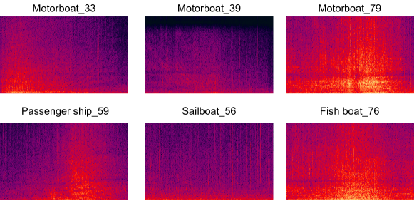
Figure 1: Spectrograms of several samples in the Shipsear dataset. Motorboat_33 records the start and stop of the motorboat “Dud”; Motorboat_39 records the arrival of the motorboat “Dud”; Motorboat_79 records the passing of the motorboat “Zodiac”; Passenger ship_59 records “Marde Mouro” sailing towards the port with considerable speed; Sailboat_56 records a sailboat passing in a very close distance; Fishboat_76 records the fish boat passing.

Despite notable advancements on open-source datasets, the performance of recognition models in practical underwater scenarios remains unsatisfactory  (Xie et al., 2022c). This can be attributed to the complexity of underwater acoustic signals, which are influenced by various interference factors, including intricate underwater environments, unpredictable transmission channels, and volatile vessel motion states (Erbe et al., 2019). Besides, variations in propeller and engine technology further impact the acoustic characteristics of radiated noise (Khishe and Mosavi, 2020). These interference factors contribute to the complexity and indistinguishability of collected signals, leading to a high intra-class diversity within the overall data distribution. Figure 1 visually illustrates the spectrogram comparisons of several samples from the Shipsear dataset, clearly demonstrating significant intra-class diversity in spectrograms among motorboats with different motion states (e.g., No.33 indicating start and stop and No.39 indicating arrival) and types (e.g., No.33 representing the motorboat “Dud” and No.79 representing the motorboat “Zodiac”). According to related studies (Schutz et al., 2013), intra-class diversity can result in potential misrecognition, particularly when data is limited.

Moreover, underwater targets (e.g., vessels) often share similar vibrational modes, such as propeller cavitation noise, and rhythm modulation noise caused by diesel piston movement. This similarity can lead to commonalities among different target categories. As observed in the spectrograms presented in Figure 1, passenger ships, sailboats, and fish boats exhibit a certain degree of similarity with motorboats. Addressing this inter-class similarity requires models to delve into high-level semantic concepts with discernible characteristics, which introduces the risk of overfitting and further complicates the recognition task.

Currently, existing literature rarely focuses on the distribution characteristics of intra-class diversity and inter-class similarity in underwater acoustic signals. For such complex signals, a natural idea is to increase the number of parameters of the model to support complex modeling. However, the scarcity of underwater data imposes significant limitations as complex models can exacerbate the overfitting phenomenon.

1.3 Our Work

In this work, we present innovative techniques to address the aforementioned challenges in underwater acoustic recognition. To mitigate the impact of intra-class diversity, it is necessary to develop an adaptive model capable of effectively processing diverse data. Drawing inspiration from successful applications of the mixture of experts (MoE) paradigm in computer vision (Ahmed et al., 2016; Riquelme et al., 2021) and natural language processing (Fedus et al., 2021; Xie et al., 2022a), we propose the convolution-based mixture of experts (referred to as CMoE) for underwater acoustic target recognition. CMoE incorporates multiple expert layers and a routing layer, where the routing layer dispatches inputs to the most suitable expert layer based on high-level representations. This approach enables adaptive disassembly of diverse data, allowing the model to learn underwater acoustic signals with multiple independent parameter spaces. Furthermore, to address the issue of inter-class similarity, we position the expert layers in the final layer of the model. It allows expert layers to learn from high-level semantic concepts and focus on discriminative characteristics within data that exhibit inter-class similarity.

Additionally, we introduce balancing regularization to handle the load balance problem and optimize our CMoE structure by incorporating an optional residual module. Experiments demonstrate that our CMoE can consistently achieve superior performance across various underwater acoustic databases. The contributions of our work can be summarized as follows:

• we reveal the unique characteristics of underwater acoustic signals, including intra-class diversity and inter-class similarity, along with the limitations of existing approaches;

• we propose the convolution-based mixture of experts to unravel complex data diversity, which captures latent characteristics from high-level representations and adaptively learns diverse data with multiple independent parameter spaces;

• we optimize our CMoE structure through balancing regularization and the incorporation of an optional residual module;

• we provide detailed visualizations and corresponding analyses of the recognition results and the routing assignment of expert layers.

2 Related Works

2.1 Underwater Acoustic Target Recognition

The research on underwater acoustic target recognition primarily revolves around acoustic feature extraction and applications of recognition algorithms. Early studies employed classic machine learning techniques to process manually designed low-dimensional acoustic features. For instance, Das et al. (Das et al., 2013) utilized cepstral features with cepstral liftering and Gaussian mixture models (GMMs) for marine vessel classification; Wang and Zeng (Wang and Zeng, 2014) employed bark-wavelet analysis in combination with the Hilbert-Huang transform to analyze signals, and employed support vector machines (SVMs) as the classifier. Moreover, cepstrum-based acoustic features from the audio and speech domains, such as Mel frequency cepstrum coefficients (MFCCs), have also yielded promising results in ship-radiated noise recognition tasks (Zhang et al., 2016; Khishe and Mohammadi, 2019). However, recent studies have revealed limitations in the general applicability of recognition systems in complex underwater scenarios when relying solely on manually designed low-dimensional acoustic features (Irfan et al., 2021; Xie et al., 2022c). Moreover, classical machine learning models may struggle to achieve satisfactory performance when confronted with large-scale data with diverse feature spaces (Irfan et al., 2021). As a result, recognition systems based on these classic paradigms face challenges in accurately recognizing unseen data in practical ocean scenarios.

With the development of deep learning (LeCun et al., 2015) and the accumulation of open-source underwater acoustic databases (Irfan et al., 2021; Santos-Domínguez et al., 2016), recognition algorithms based on deep neural networks have gained prominence. As reported in the literature, Zhang et al. (Zhang et al., 2021) utilized the short-time Fourier transform (STFT) amplitude spectrum, STFT phase spectrum, and bispectrum features as inputs for convolutional neural networks; Liu et al. (Liu et al., 2021) employed convolutional recurrent neural networks with 3-D Mel-spectrograms and data augmentation for underwater target recognition; Xie et al. (Xie et al., 2022b) utilized learnable fine-grained wavelet spectrograms with the deep residual network (ResNet) (He et al., 2016) to adaptively recognize ship-radiated noise; Ren et al. (Ren et al., 2022) employed learnable Gabor filters and ResNet for constructing an intelligent underwater acoustic classification system. In contrast to classical machine learning paradigms, deep learning methods often favor acoustic features that encapsulate comprehensive information, such as time-frequency spectrograms (Liu et al., 2021; Xie et al., 2023; Xu et al., 2023). The large number of parameters and complex nonlinearities in neural networks enable the model to effectively exploit information contained within comprehensive features. The superior performance on available datasets has propelled these methods to become the mainstream approach for underwater acoustic target recognition. However, deep learning-based systems exhibit limited robustness in practical application scenarios characterized by scarce and complex data. In this regard, many studies have employed techniques like denoising (Li et al., 2017; Ghavidel et al., 2022) and data augmentation(Liu et al., 2021; Chen et al., 2022; Xu et al., 2023) to enhance the robustness of recognition systems by improving data quality or quantity. According to our research, we are the first to address the intra-class diversity and inter-class similarity of underwater signals, and take it as the starting point for building a robust recognition system.

2.2 Mixture of Experts

To efficiently and effectively recognize complexly distributed underwater signals, this work draws inspiration from the Mixture of Experts (MoE) approach. MoE enables discriminative processing of diverse-distributed data while minimizing the introduction of excessive parameters that could lead to overfitting. The original formulation of MoE models was introduced by Jacobs et al. (Jacobs et al., 1991), including a variable number of expert models and a single gate to combine their outputs. Subsequent work by Collobert et al. (Collobert et al., 2002, 2003) applied the MoE concept to classic machine learning algorithms like support vector machines. In recent years, Shazeer et al. (Shazeer et al., 2017) explored the transition to conditional computing through sparse expert activations, wherein a fixed number of experts were activated in LSTMs. Fedus et al. (Fedus et al., 2021) extended the MoE structure to large-scale Transformers (Vaswani et al., 2017), revealing its potential to construct scalable models with reasonable overhead. As research on MoE deepened, various studies applied it to scale up Transformers (Fedus et al., 2021; Xie et al., 2022a; Rajbhandari et al., 2022; Riquelme et al., 2021) and convolutional neural networks (Gross et al., 2017; Ahmed et al., 2016; Wang et al., 2020). The sparse-gated MoE significantly increases model capacity while incurring minimal compute overhead, leading to remarkable achievements in natural language processing and computer vision. In this work, we propose a specialized convolutional MoE with sparsely-activated experts for underwater acoustic target recognition, making us the first, to the best of our knowledge, to apply the mixture of experts in this domain.

3 Methodology

This section begins by presenting the acoustic feature extraction methods employed in this work. Following that, we introduce the front-end backbone network, the expert layers, the routing layer, and the optional residual module of CMoE, respectively. Finally, we introduce the balanced regularization strategy adopted to address the load imbalance problem inherent in the MoE structure.

3.1 Acoustic Feature Extraction

In order to validate the generalizability of our proposed strategies, we employ four feature extraction techniques in this study. For raw signals, we begin by computing the spectrums through framing, windowing, and short-time Fourier transform (STFT). Subsequently, the real component is extracted and integrated across the time dimension to derive the STFT spectrogram. Following this, we employ Mel (Bark) filter banks to perform the filtering on the framed spectrums. Equation (1) illustrates that the Mel (Bark) filter bank comprises a set of bandpass filters, distributed based on the non-linear Mel (Bark) scale. Notably, the Mel (Bark) filter banks exhibit higher density at low frequencies to achieve enhanced frequency resolution. Finally, the filtered spectrums undergo conversion to Mel (Bark) spectrograms through a logarithmic scale and the integration across the time dimension.

$$Mel(f)=2595\times log(1+\frac{f}{700}),$$ (1)

$$Bark(f)=6\times arsinh(\frac{f}{600}).$$

Furthermore, we acquire the CQT spectrogram by conducting the Constant Q Transform. This involves convolving the spectrum of each frame, obtained from STFT, with the CQT kernel. The CQT kernel consists of a bank of bandpass filters that are logarithmically spaced in frequency. The $k-$th frequency component $f_{k}$ can be formalized as depicted in Equation (2), where $b$ represents the octave resolution, and $f_{max}$ and $f_{min}$ denote the maximum and minimum frequencies to be processed, respectively.

$$CQT(f_{k})=2^{k/b}f_{min}.\quad f_{min}\leq f_{k}\leq f_{max}.$$ (2)

Then, we integrate the magnitude of the filtered spectrum across the time dimension to yield the CQT spectrogram. Notably, the CQT spectrogram exhibits higher temporal resolution at high frequencies.

3.2 Front-end Backbone Network

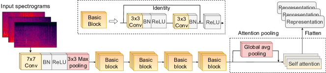
Figure 2: The model structure of the front-end backbone model - ResNet with attention pooling. “Conv” represents the convolutional layer, and “BN” represents the batch normalization layer.

Table 1: Specific network structure for our CMoE, including the front-end backbone, the expert layer and the routing layer. “num class” represents the number of classes to be predicted and “num experts” represents the number of expert layers.

Module	Specific network layer
Front-end backbone	Conv2d(1, 64, kernel size=7, stride=2, padding=3)
	Batch Normalization 2d(num features=64)
	ReLU()
	Max pooling(kernel size=3, stride=2, padding=1)
	Basic block(64,64),Basic block(64,64)
	Basic block(64,128),Basic block(128,128)
	Basic block(128,256), Basic block(256,256)
	Basic block(256,512), Basic block(512,512)
	Attention pooling(output size=(1, 1))
Basic block(in dim, out dim)	Conv2d(in dim, out dim, kernel size=3, padding=1)
	Batch Normalization 2d(num features=out dim)
	ReLU()
	Conv2d(out dim, out dim, kernel size=3, padding=1)
	Batch Normalization 2d(num features=out dim)
Expert layer	Linear(in features=512, out features=128)
	Batch Normalization 1d(num features=128)
	ReLU()
	Linear(in features=128, out features=num class)
Routing layer	Linear(in features=512, out features=num experts)

Following the feature extraction stage, we present the overall process and structure of our proposed CMoE model. Our CMoE comprises two main components. The first component is the front-end backbone network, responsible for transforming the input acoustic features into fixed-dimensional representations.

In this study, we adopt the optimized deep residual network, ResNet with attention pooling (He et al., 2016; Wang et al., 2018), as our front-end backbone. This choice is based on its superior recognition performance, as demonstrated in our preliminary experiments (see Section 5.1). The detailed structure of the front-end backbone network is illustrated in Table LABEL:tab_structure and Figure 2. It consists of a convolution layer stacked with a batch normalization (BN) layer, a ReLU layer, a max-pooling layer, followed by four residual layers and an attention pooling layer. Each residual layer comprises two basic blocks stacked together. The structure of the basic block, enclosed in a dotted box in Figure 2, includes convolution layers, BN layers, ReLU layers, and a skip connection. Mathematically, the basic block can be defined as:

$$y=F(x,\{W_{i}\})+x,$$ (3)

where $x$ and $y$ represent the input and output vectors of the basic blocks, respectively. The function $F=W_{2}\sigma(W_{1}x)$, with $\sigma$ denoting the ReLU layer and $W_{1},W_{2}$ representing the learnable mappings for the two convolutional layers. Following the residual layers, we incorporate an attention pooling layer and a flattening operation to obtain the output representations $\sim\mathbb{R}^{batchsize\times 512}$. The attention pooling layer incorporates global average pooling and multi-head self-attention operations, allowing for the assignment of dynamic weights to different regions of the feature map. This approach helps in focusing on useful information and improving the quality of the representations. The output representations from the front-end backbone network are then passed to subsequent layers in the network.

3.3 Expert Layer, Routing Layer, and Residual Module

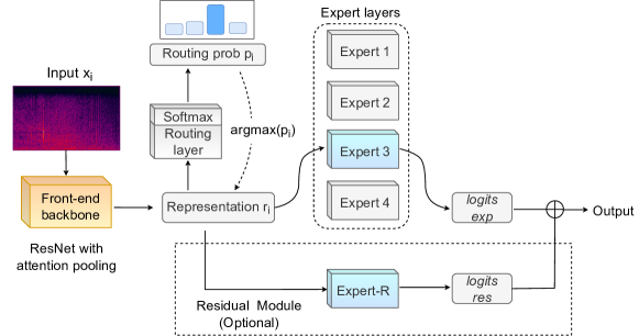
Figure 3: The overall process of our proposed CMoE, including routing probability calculation, expert assignment, and optional residual module.

The structure and training pipeline of the expert layers and the routing layer are presented in Table LABEL:tab_structure and Figure 3 respectively. Both the expert layers and the routing layer take the output representations of the front-end backbone network as input. The expert layer consists of a multi-layer perceptron with two linear layers (see Table LABEL:tab_structure). Each expert has a consistent structure, but its parameters are independent. Activation of each expert occurs only when suitable input is encountered, facilitating fine-grained and differentiated learning of diverse underwater data. The routing layer consists of a simple linear layer that adaptively guides the assignment of inputs by calculating the routing probability. This design enables the model to disassemble diverse underwater acoustic data using multiple independent parameter spaces, thereby reducing the impact of intra-class diversity. The following paragraph provides a formulaic description of the detailed process.

Let’s denote the batch size as $n$, input spectrograms as $\{x_{i}\}$, the corresponding label as $\{y_{i}\}$ (i=1,2…$n$), the number of expert layers as $m$, and the expert layers as $E_{1}(\cdot),...E_{m}(\cdot)$. The front-end backbone model first takes $x_{i}$ as input and produces high-level representations $r_{i}\sim\mathbb{R}^{n\times 512}$. These representations $r_{i}$ are then fed into the linear routing layer $G(\cdot)$, sequentially obtaining the routing score $s_{i}=G(r_{i})\sim\mathbb{R}^{1\times m}$. Then, we apply the softmax function to normalize the routing score $s_{i}$ into the routing probability $p_{i}\sim\mathbb{R}^{1\times m}$, which indicates the probability of dispatching the sample $x_{i}$ to each expert.

$$p_{i}=softmax(G(r_{i})),\quad i\epsilon[1,n]$$ (4)

$$logits_{exp}=E_{argmax(p_{i})}(r_{i}).$$

Then, the model sends the representation $r_{i}$ to the expert layer with the highest corresponding probability value. The overall routing assignment process is described in Equation (4). Take the CMoE composed of 4 experts as an example, when $p_{i}$=(0.1, 0.2, 0.4, 0.3), the corresponding representation $r_{i}$ should be sent to $E_{3}(\cdot)$ with the maximum probability.

Furthermore, to prevent overfitting from affecting routing assignment and model performance, we adopt the concept of residual connection and propose Residual CMoE (RCMoE). As depicted in Figure 3 (the dashed box at the bottom), RCMoE retains the structure of CMoE while adding an additional fixed expert layer $E_{R}(\cdot)$. The representation $r_{i}$ is directly fed into the fixed expert layer without performing routing calculations, generating $logits_{res}=E_{R}(r_{i})$. Finally, $logits_{res}$ is added to the output of the expert layers $logits_{exp}$ to obtain the overall logits. The optimization goal is to minimize the cross-entropy loss between the overall logits and labels $\{y_{i}\}$. We provide additional pseudocode in Algorithm 1 to help better understand the training flow of CMoE and RCMoE.

Data: input spectrograms $\mathcal{X}=\{x_{i}\}$; label $\mathcal{Y}=\{y_{i}\}$.

Input: number of experts $m$; batch size $n$; front-end model $F$; routing layer $G$; experts $E_{1}(\cdot),...E_{m}(\cdot)$; fixed expert $E_{R}(\cdot)$.

1 while not done do

2       Sample batches $(x_{i},y_{i})\sim(\mathcal{X,Y})$.  $i=1,2,...,n$

3       for $(x_{i},y_{i})$ do

4             # compute representations

5             $r_{i}=F(x_{i})$

6             # compute routing probabilities

7             $p_{i}=softmax(G(r_{i}),dim=-1)$

8             # dispatch $r_{i}$ to experts

9             for $1\leq i\leq n$ do

10                   $logits\ exp[i,:]=E_{argmax(p_{i})}(r[i,:])$

11                   $logits\ res[i,:]=E_{R}(r[i,:])$

12             end

13            # compute final logits

14             $logits$ = $logits\ exp$ for CMoE

15            

16            $logits$ = $(logits\ exp+logits\ res)$ for RCMoE

17       end

18      Update weights with loss $\mathcal{L}_{CE}$ = Cross Entropy$(logits,\{y_{i}\}).$

19 end while

Algorithm 1 Training flow of our (R)CMoE.

3.4 Balancing Regularization

During training, a significant issue of load imbalance arises among experts, as noted by Shazeer et al. (Shazeer et al., 2017). This imbalance manifests when a small number of experts receive the majority of inputs, while many other experts remain inadequately trained. To address this concern, we adopt the balancing regularization approach proposed by Fedus et al. (Fedus et al., 2021), aiming to promote a more equitable distribution of the workload across all experts. We inherit the notation used in the previous subsection, the balance loss is computed as follows:

$$\mathscr{L}_{balance}=\alpha m\cdot\sum_{j=1}^{m}ef_{j}\cdot ep_{j},$$ (5)

where $ef_{j}$ is represents the fraction of inputs dispatched to the $j$-th expert. We denote the number of inputs dispatched to the $j$-th expert as $Count_{j}$, thus $ef_{j}$ can be calculated as $ef_{j}=\frac{Count_{j}}{n}$. Additionally, $ep_{j}$ corresponds to the average routing probability dispatched to the $j$-th expert within the batch. It is determined by averaging the routing probabilities across the batch:

$$ep_{j}=\frac{1}{n}\sum_{i=1}^{n}p_{i}[j],$$ (6)

where $p_{i}[j]$ denotes the routing probability of dispatching token $x_{i}$ to the $j$-th expert. The balancing regularization term in Equation (5) encourages uniform routing, as minimizing it favors a uniform distribution. To control the impact of the balancing regularization during training, we introduce a hyper-parameter $\alpha$ as a coefficient for the regularization term. In this work, we set $\alpha=10^{-2}$ as the default value, striking a balance between ensuring load balancing and avoiding excessive interference with the primary cross-entropy objective. Thus, the overall training objective can be presented as follows:

$$\mathcal{L} =\mathcal{L}_{CE}+\mathcal{L}_{balance}$$ (7)

$$=Cross\ Entropy(logits,y)+\alpha m\cdot\sum_{j=1}^{m}ef_{j}\cdot ep_{j}.$$

4 Experiment Setup

4.1 Datasets

In this work, we utilize three distinct datasets of underwater ship-radiated noise at varying scales. The detailed information is provided in Table LABEL:tab1 and the subsequent paragraphs.

1. Shipsear (Santos-Domínguez et al., 2016) is an open-source database of underwater recordings of ship and boat sounds. The database comprises 90 records from 11 different vessel types, totaling nearly three hours of duration. To ensure an adequate amount of records for the “train, validation, test” split, we have selected a subset of 9 categories (dredger, fish boat, motorboat, mussel boat, natural noise, ocean liner, passenger ship, ro-ro ship, sailboat) from the Shipsear database for the recognition task.

2. Our private dataset (Ren et al., 2019) - DTIL is collected from Thousand Island Lake, which contains multiple sources of interference. It contains 330 minutes of speedboat recordings and 285 minutes of experimental vessel recordings.

3. DeepShip (Irfan et al., 2021) is an open-source underwater acoustic benchmark dataset, which consists of 47.07 hours of real-world underwater recordings of 265 different ships belonging to four classes: cargo ship, passenger ship, tanker, and tugboat.

4.2 Effective Frequency Bands

To reduce the redundancy of acoustic features, we apply effective frequency bands as substitutes for full bands during feature extraction. It involves performing a time-frequency transformation within the bandwidth that encompasses the most relevant frequency components. By doing so, we aim to reduce redundant components in input features while simultaneously reducing time and hardware consumption. Considering that the useful energy of signals predominantly concentrates on distinct frequency ranges in Shipsear, DTIL, and DeepShip, we establish independent effective frequency bands for each dataset (refer to Table LABEL:tab1). It is worth mentioning that the upper limit of the effective frequency band must be set below half of the sample rate according to the Nyquist theory. Further details about the experiments conducted to determine the optimal effective frequency band selection can be found in Section 5.1. Additionally, Table LABEL:tab1 also presents the dimensions of each acoustic feature on the three datasets.

Table 2: Information of the three datasets. “sr” represents the sampling rate and “dim” represents the feature dimensions.

dataset	duration (hours)	sr (Hz)	efficient band (Hz)	STFT dim	Mel dim	Bark dim	CQT dim
Shipsear	2.94	52734	100-26367	1200,1318	1200,300	1200,300	900,340
DTIL	10.25	17067	100-2000	1200,99	1200,300	1200,300	900,230
Deepship	47.07	32000	100-8000	1200,400	1200,300	1200,300	900,290

4.3 Data Division

In this work, each signal is cut into 30-second segments with a 15-second overlap. To prevent information leakage, we ensure that segments in the training set and the test set do not originate from the same audio track. This precautionary measure guarantees that the reported accuracy truly reflects the system’s recognition ability and generalization performance, rather than its memory capacity.

We find that almost all previous works on underwater acoustic target recognition have not disclosed their train-test splits, making it challenging to establish fair comparisons. To address this issue, we provide our carefully selected train-test splits for Shipsear (see Table 3) and DeepShip (see Table 4). 15% of the data from the training set is randomly taken as the validation set. Our manual selection principle is to ensure that the correlation between the test data and the training data is minimal. By releasing this benchmark, we aim to establish a reliable reference for future research endeavors seeking fair comparisons in this field.

Table 3: Train-test split for Shipsear. The “ID” in the table refers to the ID of the .wav file in the dataset.

Category	ID in Training set	ID in Test set
Dredger	80,93,94,96	95
Fish boat	73,74,76	75
Motorboat	21,26,33,39,45,51,52,70,77,79	27,50,72
Mussel boat	46,47,49,66	48
Natural noise	81,82,84,85,86,88,90,91	83,87,92
Ocean liner	16,22,23,25,69	24,71
Passenger ship	06,07,08,10,11,12,14,17,32,34,36,38,40,	9,13,35,42,55,62,65
	41,43,54,59,60,61,63,64,67
RO-RO ship	18,19,58	20,78
Sailboat	37,56,68	57

Table 4: Train-test split for DeepShip. The “ID” in the table refers to the ID of the .wav file in the dataset.

Category	ID in Training set	ID in Test set
Cargo ship	Else	01,02,04,05,18,30,32,35,40,48,56,62,
		63,67,68,72,74,79,83,91,92,93,95,97,
		100,104
Passenger ship	Else	02,24,25,27,11,15,17,19,20,23,30,31,
		37,45,46,52,53,60,61,62,64,67,68,70,
		75,76,77,84,86,91,101,106,113,117,122,
		125,129,130,134,135,142,144,152,157,
		159,161,167,168,177,179,187,188,189
Tanker	Else	02,03,04,07,08,13,14,15,19,22,25,28,
		35,37,46,58,62,71,73,79,82,84,88,89,
		92,99,106,115,118,124,126,127,131,134,
		141,144,147,151,153,156,158,167,171,
		178,179,185,186,190,192,193,201,205,
		213,217,228,233
Tugboat	Else	07,08,18,20,24,25,27,29,32,33,37,39,
		40,44,45,56,59,70

4.4 Parameter Setup

In this work, The frame length is set to 50ms and the frame shift defaults to half the frame length. We conduct experiments to investigate the effect of frame length on recognition results, as detailed in Section 5.1. Additionally, as a default, the number of Mel or Bark filter banks is set to 300.

During training, we employ the AdamW (Loshchilov and Hutter, 2017) optimizer with weight decay. The maximum learning rate is set to 5$\times 10^{-4}$, and the weight decay is set to $10^{-5}$ for all experiments. The models are trained for 200 epochs on A40 GPUs.

5 Results and Analyses

For the multi-class recognition task addressed in this work, we uniformly adopt the accuracy rate as the evaluation metric, which is determined by dividing the number of correctly predicted samples by the total number of samples. Besides, given the limited number of audio files in the test set, multiple groups of experiments yield the same file-level accuracy. Consequently, we present results at the segment level (30 seconds) rather than the file level. Moreover, to mitigate randomness, all reported results represent the average of experimental outcomes obtained using two distinct random seeds (42 and 123).

In this section, we initially conduct preliminary experiments on the frame length, effective frequency bands, and the structure of the front-end backbone network. After that, we perform main experiments to validate the effectiveness of CMoE based on four acoustic features and compare the experimental results with various advanced methods. This part also encompasses ablation experiments concerning the optional residual module and balancing regularization. We then provide a comprehensive visualization analysis of the expert assignment to further demonstrate the effective capture of useful information by the experts. Lastly, we carry out relevant experiments on the number of expert layers and the selection of the normalization function.

5.1 Preliminary Experiments

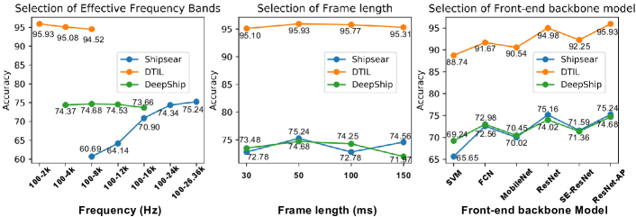
Figure 4: Preliminary experiments on the selection of effective frequency bands, frame lengths, and front-end backbone models. The frame shift is set to half the frame length by default.

Before validating CMoE, we conduct preliminary experiments on the effective frequency bands, frame length, and structure of the front-end backbone network. The detailed results are presented in Figure 4. Regarding the selection of effective frequency bands, relevant experiments consistently employ the STFT spectrogram as the input feature, utilize ResNet with attention pooling (ResNet-AP) as the model, and set the frame length to 50ms. A lower-cut-off frequency of 100Hz is set to filter out frequency bands with low signal-to-noise ratios. Experimental results indicate that Shipsear, DTIL, and DeepShip are suitable for utilizing 100-26.36kHz (Nyquist frequency), 100-2 kHz, and 100-8 kHz as effective frequency bands, respectively. For the selection of frame length, we also uniformly employ the STFT spectrogram as the input feature and ResNet-AP as the model. Optimal performance is consistently achieved with a frame length of 50ms across the three datasets. Therefore, a default frame length of 50ms is established.

Next, a comparison is made among six different backbone models - Support Vector Machine (SVM), Fully Convolutional Network (FCN), MobileNet-v3 (Howard et al., 2019), ResNet (He et al., 2016), SE-ResNet (Hu et al., 2018), and ResNet with attention pooling (ResNet-AP) (Wang et al., 2018) - for the selection of the backbone model. Among them, ResNet-AP demonstrates the highest recognition accuracy across the three datasets. Consequently, ResNet-AP is uniformly adopted as the default front-end backbone model in subsequent experiments.

5.2 Main Results of CMoE

Table 5: Main results of CMoE on four acoustic features. The “Baseline model” refers to the ResNet-AP selected in the preliminary experiments. Ablation experiments on the balancing regularization and the residual module are also included.

Dataset	Model	STFT	Mel	Bark	CQT
Shipsear	AGNet (Xie et al., 2022b)	85.48	-	-	-
	Smooth-ResNet (Xu et al., 2023)	81.90	82.76	-	75.86
	Baseline model	75.24	77.14	72.86	73.33
	CMoE	84.91	83.59	81.33	80.48
	CMoE+balance	86.21	85.35	84.48	82.76
	RCMoE+balance	85.34	84.48	83.62	82.76
DTIL	AGNet	95.76	-	-	-
	TDNN& WPCS (Ren et al., 2019)	95.31	-	-	-
	Baseline model	95.93	95.48	96.30	96.48
	CMoE	96.61	95.48	96.05	97.04
	CMoE+balance	97.89	97.46	96.89	97.88
	RCMoE+balance	98.17	97.60	97.18	97.89
DeepShip	AGNet	77.09	-	-	-
	Smooth-ResNet (Xu et al., 2023)	76.38	77.05	-	78.25
	SCAE (Irfan et al., 2021)	-	70.18	-	77.53
	Baseline model	74.68	74.85	75.15	77.82
	CMoE	75.65	76.09	76.95	77.09
	CMoE+balance	76.33	76.72	77.27	79.62
	RCMoE+balance	76.80	76.60	77.50	78.76

Then, we experimentally validate the performance of our CMoE approach. To demonstrate its superiority, we compare our results with several existing advanced methods (AGNet (Xie et al., 2022b), smoothness-inducing regularization (Xu et al., 2023), TDNN and WPCS (Ren et al., 2019), SCAE (Irfan et al., 2021)) on three datasets. The main results of our experiments are presented in Table 5. It is observed that vanilla CMoE can generally improve the recognition accuracy. Nevertheless, there are instances where the performance of CMoE may degrade due to the load imbalance issue, which is discussed in subsection 3.4. As an illustration, the CQT-based CMoE model experiences a 0.73% decrease in accuracy compared to the baseline model on DeepShip. This decrease can be attributed to the under-training of certain experts caused by the load imbalance. Notably, this problem has the risk of worsening as the number of experts increases.

With the incorporation of balancing regularization, CMoE begins to demonstrate its potential. Particularly on Shipsear, where data originates from diverse regions and exhibits varied target motion statuses, the addition of the expert layers can help model learn effectively from diverse data and significantly increase the recognition accuracy from 75.24% to 86.21%. Furthermore, it is observed that CMoE proves effective across recognition systems based on all four features, confirming its generalizability.

Furthermore, we also conduct a set of ablation experiments on the residual module (see CMoE vs. RCMoE in Table 5). It reveals that the residual module can not consistently yield improvements. RCMoE introduces a non-gated residual layer, which mitigates performance losses caused by inappropriate routing or expert overfitting. However, while addressing potential drawbacks, it also diminishes the sparsity of the network and reduces the disassembling effect of multiple expert layers on diverse data. Consequently, CMoE and RCMoE exhibit their respective strengths and weaknesses in different situations.

Figure 5: The confusion matrix heat maps of the baseline model and CMoE on Shipsear. Both models take the STFT spectrogram as the input feature.

5.3 Visualization Analyses

We proceed to use the confusion matrix heatmaps to visually illustrate the model accuracy for each category. The confusion matrix compares the predicted labels (x-axis) with the actual labels (y-axis), and the heat map represents this matrix graphically, with colors indicating the values. In Figure 5, it is evident that the baseline model’s recognition performance is unsatisfactory, with some categories (dredger, ocean liner, ro-ro ship, sailboat) achieving accuracy rates below 50%. For our proposed CMoE, the model achieves nearly 100% accuracy for several categories that were previously challenging to recognize, such as dredgers, ro-ro ships, and sailboats, indicating a promising improvement.

Figure 6: The overall assignment status of 4-expert CMoE and 8-expert CMoE on Shipsear. Both models take the STFT spectrogram as the input feature.

Then, we perform a visualization analysis of the expert assignments in Shipsear. Heat maps are used to display the results, presenting the expert assignment for CMoE models with 4 and 8 experts (see Figure 6). The colors in the heat maps represent the proportion of samples assigned to each expert category. Our analysis reveals a possible correlation between expert assignment and target size. According to experiential knowledge, ocean liners and ro-ro ships are classified as large targets, while motorboats and sailboats are considered small targets. As depicted in Figure 6, the 8-expert CMoE tends to assign both ocean liners and ro-ro ships to the No.5 expert, while motorboats and sailboats are predominantly assigned to the No.1 expert. Similarly, the 4-expert CMoE exhibits similar assignments for small and large targets. This finding suggests that the routing module may capture inherent characteristics associated with target size.

Furthermore, Figure 7 presents the expert assignments for the six samples mentioned in Figure 1. By comparing three motorboat samples with different motion states and types, we observe both overlaps and differences in their expert assignments. To some extent, the overlaps represent the target-related patterns, while the differences reflect the intra-class diversity. Additionally, we compare the expert assignment for samples from different categories with similar spectrograms (e.g., motorboat 33 vs passenger ship 59) and find that samples with similar spectrograms have different expert assignments. This suggests that our CMoE is successful in dealing with the inter-class similarity issue.

Figure 7: The expert assignment for the six samples. Since each sample can be cut into multiple 30s segments, these segments may be dispatched to multiple experts.

To conclude, the routing module responsible for expert assignment demonstrates the capability to capture target-related characteristics and intra-class diversity from high-level representations. Furthermore, we also find that the expert assignment of CMoE is little affected by inter-class similarity. The above visualization analysis provides certain interpretability for routing assignments.

5.4 Number of Experts

(a) Experiments on Shipsear.

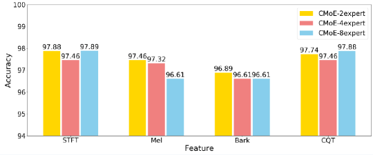
(b) Experiments on DTIL.

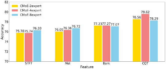
(c) Experiments on DeepShip.

Figure 8: Experiments about the number of experts with various features on three datasets.

In this subsection, we delve into the examination of the influence of the number of experts in CMoE models. Our analysis reveals that while increasing the number of experts allows for a more fine-grained understanding of the data, it also diminishes the data dispatched to each expert, thereby increasing the risk of overfitting. Consequently, selecting the optimal number of experts becomes a complex trade-off. Figure 8 presents the results for CMoE models with 2, 4, and 8 experts across three datasets. The results illustrate that the impact of the number of experts is not simply proportional but varies depending on factors such as data scale, data diversity, input features, and other considerations. Only a portion of results show obvious correlations. On DeepShip, where the training data is relatively abundant compared to the other two datasets, CMoE with 2 experts exhibits the poorest performance. This is attributed to the limited capacity of CMoE to learn from diverse data. Besides, for redundant features, such as the STFT spectrogram on Shipsear with a dimension of 1200$\times$1318, increasing the number of expert layers can enhance performance. For other sets of experiments, the coupling of multiple influencing factors complicates the discovery of clear rules.

To summarize, selecting the optimal number of experts is a multifaceted trade-off task, and the impact of the expert layer on performance is contingent upon the characteristics of the data and features. Therefore, an extensive search for the optimal number of experts through traversal becomes necessary.

5.5 Selection of the Normalization Function

Table 6: Experiments about the normalization function with various features on three datasets.

Dataset	Model	Norm func	STFT	Mel	Bark	CQT
Shipsear	CMoE	softmax	84.48	83.19	84.48	82.76
		sigmoid	86.21	85.35	84.48	80.17
	RCMoE	softmax	84.19	82.76	83.19	82.33
		sigmoid	85.34	84.48	83.62	82.76
DTIL	CMoE	softmax	97.89	97.46	96.89	97.60
		sigmoid	97.88	96.89	96.61	97.88
	RCMoE	softmax	98.17	97.18	96.89	97.89
		sigmoid	97.74	97.60	97.18	97.32
DeepShip	CMoE	softmax	76.33	76.36	76.52	79.62
		sigmoid	75.66	76.72	77.27	78.56
	RCMoE	softmax	76.80	76.60	77.50	78.76
		sigmoid	76.23	76.46	76.56	77.99

Table 6 provides an overview of the impact of normalization functions on the recognition performance of CMoE and RCMoE. Note that the probability distribution to be normalized is $p$, and the formulas for the two normalization functions are as follows:

$$Softmax(p_{i})=\frac{e^{p_{i}}}{\sum_{j=1}^{n}e^{p_{j}}}(dim=-1),$$ (8)

$$Sigmoid(p)=\frac{1}{1+e^{-p}},$$

where $p_{i}$ represents the probability distribution corresponding to the $i$-th class, while $n$ represents the total number of classes. The softmax function effectively converts the multi-category output values into a probability distribution within the range of (0, 1), where the sum of all probability values is equal to 1. On the other hand, the sigmoid function also maps the output values to the interval of (0, 1), with a steeper slope near the value of 0.5.

Upon analyzing the experimental results presented in Table 6, it becomes apparent that the performance of the two normalization functions exhibits distinct advantages and disadvantages across different features and datasets. Although both functions only serve to normalize, they possess distinct gradient properties that can influence the weight updates of the network during backpropagation. Consequently, it is challenging to determine a universally superior normalization function. Both softmax and sigmoid normalization approaches are employed in this study, and the approach that yields superior results is selected.

6 Conclusion

This work unveils the uniqueness of underwater acoustic signals, characterized by high intra-class diversity and inter-class similarity. Building upon this foundation, we propose an innovative application of the mixture of experts to underwater acoustic recognition, called CMoE. This technique captures latent characteristics from high-level representations and adaptively learns diverse data with multiple independent parameter spaces. To optimize our model, we further incorporate balancing regularization and a residual module. Through comprehensive experiments, we demonstrate the superiority of our proposed method and underscore the necessity of balancing regularization. Furthermore, visualization analysis validates the effectiveness of our approach and enhances interpretability of the model.

Despite promising results, our CMoE still leaves certain limitations. First, we show that the assignment of experts is related to the intrinsic properties of targets (e.g., target size) to a certain extent, but the phenomenon lacks sufficient theoretical support. Moreover, the design of the structure of expert layers and routing layer is relatively simple. We believe that the current CMoE with simple linear layers as the experts or the routing layer does not fully exploit the potential of the MoE structure. In our future work, we aim to investigate the potential of utilizing physically-based target characteristics, such as the number of propeller blades, as the foundation for routing instead of relying solely on the automatically learned routing layer. This approach offers improved interpretability and holds promise for our research endeavors.

References

- Ahmed et al. (2016) Ahmed, K., Baig, M.H., Torresani, L., 2016. Network of experts for large-scale image categorization, in: Computer Vision–ECCV 2016: 14th European Conference, Amsterdam, The Netherlands, October 11–14, 2016, Proceedings, Part VII 14, Springer. pp. 516–532.
- Chen et al. (2021) Chen, J., Han, B., Ma, X., Zhang, J., 2021. Underwater target recognition based on multi-decision lofar spectrum enhancement: A deep-learning approach. Future Internet 13, 265.
- Chen et al. (2022) Chen, L., Liu, F., Li, D., Shen, T., Zhao, D., 2022. Underwater acoustic target classification with joint learning framework and data augmentation, in: 2022 5th International Conference on Artificial Intelligence and Big Data (ICAIBD), IEEE. pp. 23–28.
- Collobert et al. (2002) Collobert, R., Bengio, S., Bengio, Y., 2002. A parallel mixture of svms for very large scale problems. Neural computation 14, 1105–1114.
- Collobert et al. (2003) Collobert, R., Bengio, Y., Bengio, S., 2003. Scaling large learning problems with hard parallel mixtures. International Journal of pattern recognition and artificial intelligence 17, 349–365.
- Das et al. (2013) Das, A., Kumar, A., Bahl, R., 2013. Marine vessel classification based on passive sonar data: The cepstrum-based approach. IET Radar, Sonar & Navigation 7, 87–93.
- Erbe et al. (2019) Erbe, C., Marley, S.A., Schoeman, R.P., Smith, J.N., Trigg, L.E., Embling, C.B., 2019. The effects of ship noise on marine mammals—a review. Frontiers in Marine Science 6, 606.
- Erkmen and Yıldırım (2008) Erkmen, B., Yıldırım, T., 2008. Improving classification performance of sonar targets by applying general regression neural network with pca. Expert Systems with Applications 35, 472–475.
- Fedus et al. (2021) Fedus, W., Zoph, B., Shazeer, N., 2021. Switch transformers: Scaling to trillion parameter models with simple and efficient sparsity. The Journal of Machine Learning Research 23, 1–40.
- Ghavidel et al. (2022) Ghavidel, M., Azhdari, S.M.H., Khishe, M., Kazemirad, M., 2022. Sonar data classification by using few-shot learning and concept extraction. Applied Acoustics 195, 108856.
- Gross et al. (2017) Gross, S., Ranzato, M., Szlam, A., 2017. Hard mixtures of experts for large scale weakly supervised vision, in: Proceedings of the IEEE Conference on Computer Vision and Pattern Recognition, pp. 6865–6873.
- He et al. (2016) He, K., Zhang, X., Ren, S., Sun, J., 2016. Deep residual learning for image recognition, in: Proceedings of the IEEE conference on computer vision and pattern recognition, pp. 770–778.
- Hovem (2012) Hovem, J.M., 2012. Marine acoustics: The physics of sound in underwater environments. Peninsula publishing Los Altos, CA.
- Howard et al. (2019) Howard, A., Sandler, M., Chu, G., Chen, L.C., Chen, B., Tan, M., Wang, W., Zhu, Y., Pang, R., Vasudevan, V., et al., 2019. Searching for mobilenetv3, in: Proceedings of the IEEE/CVF international conference on computer vision, pp. 1314–1324.
- Hu et al. (2018) Hu, J., Shen, L., Sun, G., 2018. Squeeze-and-excitation networks, in: Proceedings of the IEEE conference on computer vision and pattern recognition, pp. 7132–7141.
- Irfan et al. (2021) Irfan, M., Jiangbin, Z., Ali, S., Iqbal, M., Masood, Z., Hamid, U., 2021. Deepship: An underwater acoustic benchmark dataset and a separable convolution based autoencoder for classification. Expert Systems with Applications 183, 115270.
- Jacobs et al. (1991) Jacobs, R.A., Jordan, M.I., Nowlan, S.J., Hinton, G.E., 1991. Adaptive mixtures of local experts. Neural computation 3, 79–87.
- Jia et al. (2022) Jia, H., Khishe, M., Mohammadi, M., Rashidi, S., 2022. Deep cepstrum-wavelet autoencoder: A novel intelligent sonar classifier. Expert Systems with Applications 202, 117295.
- Ke et al. (2020) Ke, X., Yuan, F., Cheng, E., 2020. Integrated optimization of underwater acoustic ship-radiated noise recognition based on two-dimensional feature fusion. Applied Acoustics 159, 107057.
- Khishe (2022) Khishe, M., 2022. Drw-ae: A deep recurrent-wavelet autoencoder for underwater target recognition. IEEE Journal of Oceanic Engineering 47, 1083–1098.
- Khishe and Mohammadi (2019) Khishe, M., Mohammadi, H., 2019. Passive sonar target classification using multi-layer perceptron trained by salp swarm algorithm. Ocean Engineering 181, 98–108.
- Khishe and Mosavi (2020) Khishe, M., Mosavi, M., 2020. Classification of underwater acoustical dataset using neural network trained by chimp optimization algorithm. Applied Acoustics 157, 107005.
- LeCun et al. (2015) LeCun, Y., Bengio, Y., Hinton, G., 2015. Deep learning. nature 521, 436–444.
- Li et al. (2017) Li, Y., Li, Y., Chen, X., Yu, J., 2017. Denoising and feature extraction algorithms using npe combined with vmd and their applications in ship-radiated noise. Symmetry 9, 256.
- Liu et al. (2021) Liu, F., Shen, T., Luo, Z., Zhao, D., Guo, S., 2021. Underwater target recognition using convolutional recurrent neural networks with 3-d mel-spectrogram and data augmentation. Applied Acoustics 178, 107989.
- Loshchilov and Hutter (2017) Loshchilov, I., Hutter, F., 2017. Decoupled weight decay regularization. arXiv preprint arXiv:1711.05101 .
- Rajbhandari et al. (2022) Rajbhandari, S., Li, C., Yao, Z., Zhang, M., Aminabadi, R.Y., Awan, A.A., Rasley, J., He, Y., 2022. Deepspeed-moe: Advancing mixture-of-experts inference and training to power next-generation ai scale, in: International Conference on Machine Learning, PMLR. pp. 18332–18346.
- Ren et al. (2019) Ren, J., Huang, Z., Li, C., Guo, X., Xu, J., 2019. Feature analysis of passive underwater targets recognition based on deep neural network, in: OCEANS 2019-Marseille, IEEE. pp. 1–5.
- Ren et al. (2022) Ren, J., Xie, Y., Zhang, X., Xu, J., 2022. Ualf: A learnable front-end for intelligent underwater acoustic classification system. Ocean Engineering 264, 112394.
- Riquelme et al. (2021) Riquelme, C., Puigcerver, J., Mustafa, B., Neumann, M., Jenatton, R., Susano Pinto, A., Keysers, D., Houlsby, N., 2021. Scaling vision with sparse mixture of experts. Advances in Neural Information Processing Systems 34, 8583–8595.
- Saffari et al. (2023) Saffari, A., Zahiri, S.H., Khishe, M., 2023. Fuzzy whale optimisation algorithm: a new hybrid approach for automatic sonar target recognition. Journal of Experimental & Theoretical Artificial Intelligence 35, 309–325.
- Santos-Domínguez et al. (2016) Santos-Domínguez, D., Torres-Guijarro, S., Cardenal-López, A., Pena-Gimenez, A., 2016. Shipsear: An underwater vessel noise database. Applied Acoustics 113, 64–69.
- Schutz et al. (2013) Schutz, A., Bombrun, L., Berthoumieu, Y., 2013. K-centroids-based supervised classification of texture images: Handling the intra-class diversity, in: 2013 IEEE International Conference on Acoustics, Speech and Signal Processing, IEEE. pp. 1498–1502.
- Shazeer et al. (2017) Shazeer, N., Mirhoseini, A., Maziarz, K., Davis, A., Le, Q., Hinton, G., Dean, J., 2017. Outrageously large neural networks: The sparsely-gated mixture-of-experts layer. arXiv preprint arXiv:1701.06538 .
- Simonović et al. (2021) Simonović, M., Kovandžić, M., Ćirić, I., Nikolić, V., 2021. Acoustic recognition of noise-like environmental sounds by using artificial neural network. Expert Systems with Applications 184, 115484.
- Sutin et al. (2010) Sutin, A., Bunin, B., Sedunov, A., Sedunov, N., Fillinger, L., Tsionskiy, M., Bruno, M., 2010. Stevens passive acoustic system for underwater surveillance, in: 2010 International WaterSide Security Conference, IEEE. pp. 1–6.
- Vaswani et al. (2017) Vaswani, A., Shazeer, N., Parmar, N., Uszkoreit, J., Jones, L., Gomez, A.N., Kaiser, Ł., Polosukhin, I., 2017. Attention is all you need. Advances in neural information processing systems 30, 2017.
- Wang and Zeng (2014) Wang, S., Zeng, X., 2014. Robust underwater noise targets classification using auditory inspired time-frequency analysis. Applied Acoustics 78, 68–76.
- Wang et al. (2018) Wang, X., Girshick, R., Gupta, A., He, K., 2018. Non-local neural networks, in: Proceedings of the IEEE conference on computer vision and pattern recognition, pp. 7794–7803.
- Wang et al. (2020) Wang, X., Yu, F., Dunlap, L., Ma, Y.A., Wang, R., Mirhoseini, A., Darrell, T., Gonzalez, J.E., 2020. Deep mixture of experts via shallow embedding, in: Uncertainty in artificial intelligence, PMLR. pp. 552–562.
- Xie et al. (2022a) Xie, Y., Huang, S., Chen, T., Wei, F., 2022a. Moec: Mixture of expert clusters. arXiv preprint arXiv:2207.09094 .
- Xie et al. (2022b) Xie, Y., Ren, J., Xu, J., 2022b. Adaptive ship-radiated noise recognition with learnable fine-grained wavelet transform. Ocean Engineering 265, 112626.
- Xie et al. (2022c) Xie, Y., Ren, J., Xu, J., 2022c. Underwater-art: Expanding information perspectives with text templates for underwater acoustic target recognition. The Journal of the Acoustical Society of America 152, 2641–2651.
- Xie et al. (2023) Xie, Y., Ren, J., Xu, J., 2023. Guiding the underwater acoustic target recognition with interpretable contrastive learning, in: OCEANS 2023-Limerick, IEEE. pp. 1–6.
- Xu et al. (2023) Xu, J., Xie, Y., Wang, W., 2023. Underwater acoustic target recognition based on smoothness-inducing regularization and spectrogram-based data augmentation. Ocean Engineering 281, 114926.
- Zhang et al. (2016) Zhang, L., Wu, D., Han, X., Zhu, Z., 2016. Feature extraction of underwater target signal using mel frequency cepstrum coefficients based on acoustic vector sensor. Journal of Sensors 2016, 7864213.
- Zhang et al. (2021) Zhang, Q., Da, L., Zhang, Y., Hu, Y., 2021. Integrated neural networks based on feature fusion for underwater target recognition. Applied Acoustics 182, 108261.