Scalable Virtual Valuations Combinatorial Auction Design by Combining Zeroth-Order and First-Order Optimization Method

Abstract

Automated auction design seeks to discover empirically high-revenue and incentive-compatible mechanisms using machine learning. Ensuring dominant strategy incentive compatibility (DSIC) is crucial, and the most effective approach is to confine the mechanism to Affine Maximizer Auctions (AMAs). Nevertheless, existing AMA-based approaches encounter challenges such as scalability issues (arising from combinatorial candidate allocations) and the non-differentiability of revenue. In this paper, to achieve a scalable AMA-based method, we further restrict the auction mechanism to Virtual Valuations Combinatorial Auctions (VVCAs), a subset of AMAs with significantly fewer parameters. Initially, we employ a parallelizable dynamic programming algorithm to compute the winning allocation of a VVCA. Subsequently, we propose a novel optimization method that combines both zeroth-order and first-order techniques to optimize the VVCA parameters. Extensive experiments demonstrate the efficacy and scalability of our proposed approach, termed Zeroth-order and First-order Optimization of VVCAs (ZFO-VVCA), particularly when applied to large-scale auctions.

1 Introduction

Finding high-revenue mechanisms that are both dominant strategy incentive compatible (DSIC) and individually rational (IR) is a fundamental problem in auction design. While the optimal auction design for the single-item case is characterized by Myerson (1981), the optimal auction design for the multi-item case remains an open problem. Despite encountering theoretical bottlenecks, automated auction design has achieved significant empirical success. This paradigm formulates auction design as an optimization problem subject to DSIC and IR constraints (Dütting et al., 2023) or restricts the auction class to be DSIC and IR (Likhodedov et al., 2005; Sandholm and Likhodedov, 2015), then seeks high-revenue solutions using machine learning.

Presently, the most effective approach to ensure DSIC and IR is to constrain the mechanism to Affine Maximizer Auctions (AMAs) (Roberts, 1979), a generalized version of Vickrey-Clarke-Groves (VCG) auctions (Vickrey, 1961). AMAs assign weights to each bidder and enhance each candidate allocation, enabling them to achieve higher revenue than VCG while ensuring DSIC. In a standard AMA, candidate allocations encompass all $(n+1)^{m}$ deterministic outcomes for $n$ bidders and $m$ items, resulting in $O((n+1)^{m})$ parameters. This extensive parameter space poses scalability challenges. Moreover, the revenue of an AMA is non-differentiable concerning its parameters, as the computation of revenue involves searching for the affine welfare-maximizing allocation.

To tackle the scalability and optimization issues of AMA-based approaches, Curry et al. (2023) and Duan et al. (2023) address the problem by limiting the size of candidate allocations to $s\ll(n+1)^{m}$ and making them learnable as well. These randomized AMAs enjoy fewer parameters, and the computation of their revenue can be approximated using differentiable operators based on the softmax function. However, the effective size of candidate allocations still grows with increased bidders and items, leading to suboptimal performance in large-scale auctions.

Another strategy to address the scalability issue is to further constrain the mechanism to Virtual Valuations Combinatorial Auctions (VVCAs) (Likhodedov et al., 2005; Sandholm and Likhodedov, 2015), a subset of AMAs. VVCAs boost each bidder-bundle pair, reducing the parameters to $O(n2^{m})$. However, similar to AMAs, VVCAs still suffer from optimization issues. The optimization processes of existing VVCA-based methods overlook the influence of VVCA parameters on the resulting winning allocations, leading to suboptimal outcomes.

To address the challenges outlined above, we introduce a novel and scalable algorithm for designing VVCA: Zeroth-order and First-order Optimization for VVCAs (ZFO-VVCA). We initiate the process by devising a GPU-friendly dynamic programming algorithm to compute the winning allocation efficiently. Following this, we partition the revenue into differentiable and non-differentiable components. The gradient of the differentiable portion is computed through differentiation. For the non-differentiable part, we employ a zeroth-order method to approximate the gradient of its Gaussian smoothing approximation. By integrating the gradients obtained through both the first-order and zeroth-order methods, we subsequently apply the standard gradient ascent method to optimize the VVCA parameters.

Finally, we conduct extensive experiments to showcase the effectiveness of ZFO-VVCA. Our revenue experiments reveal that, in most cases, ZFO-VVCA achieves higher revenue than all deterministic baselines in automated auction design and performs comparably in the remaining settings. Moreover, in large-scale auctions, ZFO-VVCA outperforms the randomized methods Lottery AMA (Curry et al., 2023) and AMenuNet (Duan et al., 2023) with acceptable candidate sizes, highlighting the scalability of ZFO-VVCA. Additionally, we perform an ablation study and a case study to demonstrate that the zeroth-order optimization component significantly benefits ZFO-VVCA from both revenue and optimization perspectives.

2 Related Work

Automated Auction Design

Research in automated auction design can be broadly categorized into two threads. The first thread, initiated by RegretNet (Dütting et al., 2019), utilizes ex-post regret as a metric to quantify the extent of DSIC violation. Building upon this concept, subsequent works such as Curry et al. (2020); Peri et al. (2021); Rahme et al. (2021b, a); Curry et al. (2022); Duan et al. (2022); Ivanov et al. (2022) represent auction mechanisms through neural networks. These models aim to achieve near-optimal and approximate DSIC solutions through adversarial training. The advantages of regret-based methods lie in their ability to attain high revenue, considering a broad class of auction mechanisms. Furthermore, this methodology is generalizable and applicable to various other mechanism design problems, including multi-facility location (Golowich et al., 2018), two-sided matching (Ravindranath et al., 2021), and data markets (Ravindranath et al., 2023). However, it is important to note that regret-based methods are not guaranteed to be DSIC, and computing the regret term can be time-consuming.

The second thread focuses on Affine Maximizer Auctions (AMAs) (Roberts, 1979), a weighted variation of the Vickrey-Clarke-Groves (VCG) mechanism. AMAs assign weights to each bidder and boost each candidate allocation, enabling them to achieve higher revenue than VCG while maintaining DSIC. This method is particularly well-suited for scenarios with limited candidate allocations (Li et al., 2024). Furthermore, the sample complexity of AMA has been characterized by Balcan et al. (2016, 2018, 2023). However, conventional AMAs encounter scalability challenges in multi-item auctions with $n$ bidders and $m$ items, given the total of $(n+1)^{m}$ deterministic candidate allocations. Additionally, an AMA’s revenue is non-differentiable regarding its parameters, as the computation involves searching for the affine welfare-maximizing allocation. One approach to address these challenges is to restrict the size of candidate allocations to $s\ll(n+1)^{m}$ and make the candidate allocations learnable (Curry et al., 2023; Duan et al., 2023). However, as discussed earlier, the effective size of candidate allocations still grows with an increasing number of bidders and items. This growth results in suboptimal performance in large-scale auctions.

Subset of AMAs

An additional strategy to address the scalability issue of AMA involves further constraining the mechanism to specific subsets, such as Virtual Valuations Combinatorial Auctions (VVCAs) (Likhodedov and Sandholm, 2004; Likhodedov et al., 2005; Sandholm and Likhodedov, 2015), $\lambda$-auctions (Jehiel et al., 2007), mixed bundling auctions (Tang and Sandholm, 2012), and bundling boosted auctions (Balcan et al., 2021). Among these options, VVCAs constitute the most significant subset. Given this, we focus on restricting the mechanism to be VVCAs. However, VVCAs still suffer from the non-differentiability of revenue. Existing VVCA-based algorithms (Likhodedov et al., 2005; Sandholm and Likhodedov, 2015) compute the “gradient” of revenue based on fixed winning allocations, neglecting the influence of VVCA parameters on the winning allocations.

Zeroth-order Optimization

Zeroth-order optimization (ZO) methods (Nesterov and Spokoiny, 2017), a subset of gradient-free optimization, are designed to tackle optimization problems where computing the gradient is either unavailable or impractical (Flaxman et al., 2004; Spall, 2005; Rao, 2019). Over time, several works have proposed ZO algorithms for intricate optimization scenarios (Ghadimi et al., 2016; Liu et al., 2020, 2018) under different constraints (Chen et al., 2019; Duchi et al., 2015; Balasubramanian and Ghadimi, 2018). The application of ZO methods has also extended to various domains, including game theory (Bichler et al., 2021) and reinforcement learning (Salimans et al., 2017).

3 Preliminary

Sealed-Bid Auction

A sealed-bid auction involves $n$ bidders denoted as $[n]=\{1,2,\dots,n\}$ and $m$ items denoted as $[m]=\{1,2,\dots,m\}$. Each bidder $i$ assigns a valuation $v_{i}(\mathcal{S})$ to every bundle of items $\mathcal{S}\subseteq[m]$ and submits bids for each bundle as ${\bm{b}}_{i}\in\mathbb{R}^{2^{m}}$. We assume $v_{i}(\emptyset)=0$ for all bidders. In the additive setting, $v_{i}(\mathcal{S})=\sum_{j\in\mathcal{S}}v_{i}(\{j\})=\sum_{j\in\mathcal{S}}v_{ij}$. The valuation profile $V=({\bm{v}}_{1},{\bm{v}}_{2},\dots,{\bm{v}}_{n})$ is generated from a distribution $D$. The auctioneer lacks knowledge of the true valuation profile $V$ but can observe the bidding profile $B=({\bm{b}}_{1},{\bm{b}}_{2},\dots,{\bm{b}}_{n})$.

Auction Mechanism

An auction mechanism $(g,p)$ consists of an allocation rule $g$ and a payment rule $p$. Given the bids $B$, $g_{i}(B)$ computes the allocation result for bidder $i$, which can be a bundle of items or a probability distribution over all the bundles. The payment $p_{i}(B)\geq 0$ computes the price that bidder $i$ needs to pay. Each bidder aims to maximize her utility, defined as $u_{i}({\bm{v}}_{i},B)\coloneqq v_{i}(g_{i}(B))-p_{i}(B)$.

Bidders may misreport their valuations to gain an advantage. Such strategic behavior among bidders could make the auction result hard to predict. Therefore, we require the auction mechanism to be dominant strategy incentive compatible (DSIC), meaning that for each bidder $i\in[n]$, reporting her true valuation is her optimal strategy regardless of how others report. Formally, let $B_{-i}=({\bm{b}}_{1},\dots,{\bm{b}}_{i-1},{\bm{b}}_{i+1},\dots,{\bm{b}}_{n})$ be the bids except for bidder $i$. A DSIC mechanism satisfies

$$u_{i}({\bm{v}}_{i},({\bm{v}}_{i},B_{-i}))\geq u_{i}({\bm{v}}_{i},({\bm{b}}_{i},B_{-i})),\quad\forall i,{\bm{v}}_{i},B_{-i},{\bm{b}}_{i}.$$ (DSIC)

Furthermore, the auction mechanism needs to be individually rational (IR), ensuring that truthful bidding results in a non-negative utility for each bidder. Formally,

$$u_{i}({\bm{v}}_{i},({\bm{v}}_{i},B_{-i}))\geq 0,\quad\forall i,{\bm{v}}_{i},B_{-i}.$$ (IR)

Affine Maximizer Auction (AMA)

AMAs (Roberts, 1979) serves as a generalized version of VCG auctions (Vickrey, 1961) and inherently ensures DSIC and IR. Typically, an AMA comprises positive weights $w_{i}\in\mathbb{R}_{+}$ for each bidder and boost variables $\lambda(A)\in\mathbb{R}$ for each candidate allocation $A\in\mathcal{A}$, where $\mathcal{A}$ is the set of all candidate allocations. In our paper, we set the candidate allocations as all the $(n+1)^{m}$ deterministic allocations.

Given bids $B$, an AMA selects the allocation that maximizes the affine welfare $\mathrm{AW}(A,B,{\bm{w}},{\bm{\lambda}})$ (with an arbitrary tie-breaking rule):

$$g(B;{\bm{w}},\bm{\lambda}) =\operatorname*{argmax}_{A\in\mathcal{A}}\mathrm{AW}(A,B,{\bm{w}},{\bm{\lambda}})=\operatorname*{argmax}_{A\in\mathcal{A}}\sum_{i=1}^{n}w_{i}b_{i}(A)+\lambda(A),$$ (1)

and each bidder $i$ pays for her normalized negative impact (with respect to affine welfare) on other bidders:

$$p_{i}(B;{\bm{w}},\bm{\lambda})=\frac{1}{w_{i}}\max_{A\in\mathcal{A}}\left(\sum_{j\neq i}w_{j}b_{j}(A)+\lambda(A)\right)-\frac{1}{w_{i}}\left(\sum_{j\neq i}w_{j}b_{j}(g(B;{\bm{w}},\bm{\lambda}))+\lambda(g(B;{\bm{w}},\bm{\lambda}))\right).$$ (2)

Since AMAs are inherently DSIC and IR, rational bidders would always truthfully bid, ensuring $B=V$.

Virtual Valuations Combinatorial Auction (VVCA)

VVCAs (Likhodedov et al., 2005) is a subset of AMAs, distinguishing itself by decomposing the boost variable of AMAs into $n$ parts, one for each bidder. Formally, a VVCA boosts per bidder-bundle pair as follows:

$$\lambda(A)=\sum_{i=1}^{n}\lambda_{i}(A_{i})$$ (3)

This decomposition results in a reduction of VVCA parameters from $O((n+1)^{m})$ to $O(n2^{m})$, aligning with the same order as the input valuation $V$.

4 Methodology

We aim to discover a high-revenue auction mechanism that satisfies both (DSIC) and (IR) for a sealed-bid auction with $n$ bidders and $m$ items. Currently, there is no known characterization of a DSIC multi-item combinatorial auction (Dütting et al., 2023), leading to a common strategy of limiting the auction class to AMAs (Likhodedov et al., 2005; Sandholm and Likhodedov, 2015; Curry et al., 2023; Duan et al., 2023).

AMAs are inherently DSIC and IR, encompassing a broad class of mechanisms (Lavi et al., 2003). However, the boost parameters $\bm{\lambda}$ are defined across the entire candidate allocations, resulting in $(n+1)^{m}$ parameters. To address the scalability challenges stemming from the parameter space, following Sandholm and Likhodedov (2015), we further constrain the auction class to VVCA.

Formally, our optimization problem is:

$$\max_{{\bm{w}},\bm{\lambda}}\leavevmode\nobreak\ {R}_{D}({\bm{w}},\bm{\lambda})\coloneqq \mathbb{E}_{V\sim D}\left[{R}(V,{\bm{w}},\bm{\lambda})\right]\coloneqq\mathbb{E}_{V\sim D}\left[\sum_{i=1}^{n}p_{i}(V;{\bm{w}},\bm{\lambda})\right].$$ (4)

Based on Equation 2 and Equation 3, $R(V,{\bm{w}},\bm{\lambda})$ can be further derived as follows:

$${R}(V,{\bm{w}},\bm{\lambda}) \overset{(a)}{\coloneqq}F(V,{\bm{w}},\bm{\lambda})+Z(V,{\bm{w}},\bm{\lambda})$$ (5)

$$\overset{(b)}{\coloneqq}\left[\sum_{i=1}^{n}\frac{1}{w_{i}}\max_{A\in\mathcal{A}}\left(\sum_{j\neq i}w_{j}v_{j}(A)+\sum_{k=1}^{n}\lambda_{k}(A_{k})\right)-\sum_{i=1}^{n}\frac{1}{w_{i}}\max_{A\in\mathcal{A}}\left(\sum_{j=1}^{n}w_{j}v_{j}(A)+\lambda_{j}(A_{j})\right)\right]$$

$$\quad+\left[\sum_{i=1}^{n}v_{i}(g(V;{\bm{w}},\bm{\lambda}))\right],$$

where in $(a)$ we define $F(V,{\bm{w}},\bm{\lambda})$ as the first two terms in $(b)$, and

$$Z(V,{\bm{w}},{\bm{\lambda}})\coloneqq\sum_{i=1}^{n}v_{i}(g(V;{\bm{w}},\bm{\lambda}))$$

as the final term in $(b)$.

Algorithm 1 Winning Allocation Determination by Dynamic Programming

1:  Input: Valuation $V$, VVCA parameters ${\bm{w}}\in\mathbb{R}_{+}^{n}$ and $\bm{\lambda}\in\mathbb{R}^{n2^{m}}$.

2:  Output: Maximum affine welfare $\mathrm{MAW}^{*}$ and the corresponding allocation $A^{*}$.

3:  for $\mathcal{S}\subseteq[m]$ do

4:     Initialize $\mathrm{MAW}(1,\mathcal{S})\leftarrow w_{1}v_{1}(\mathcal{S})+\lambda_{1}(\mathcal{S})$

5:     Initialize $\mathrm{AB}(1,\mathcal{S})\leftarrow\mathcal{S}$

6:  end for

7:  for $i=2$ to $n$ do

8:     for $\mathcal{S}\subseteq[m]$ do

9:        Denote $\mathrm{MAW}^{\prime}(i,\mathcal{S},\mathcal{B})$ as $\mathrm{MAW}(i-1,\mathcal{S}\backslash\mathcal{B})+w_{i}v_{i}(\mathcal{B})+\lambda_{i}(\mathcal{B})$ for all $\mathcal{B}\subseteq\mathcal{S}$

10:        Compute the maximum affine welfare when allocating $\mathcal{S}$ to the previous $i$ bidders:  $\mathrm{MAW}(i,\mathcal{S})\leftarrow\max_{\mathcal{B}\subseteq\mathcal{S}}\mathrm{MAW}^{\prime}(i,\mathcal{S},\mathcal{B})$

11:        Record the allocated bundle of bidder $i$:  $\mathrm{AB}(i,\mathcal{S})\leftarrow\operatorname*{argmax}_{\mathcal{B}\subseteq\mathcal{S}}\mathrm{MAW}^{\prime}(i,\mathcal{S},\mathcal{B})$

12:     end for

13:  end for

14:  $\mathrm{MAW}^{*}\leftarrow\max_{\mathcal{S}\subseteq[m]}\mathrm{MAW}(n,\mathcal{S})$.

15:  $\mathcal{S}_{n}\leftarrow\operatorname*{argmax}_{\mathcal{S}\subseteq[m]}\mathrm{MAW}(n,\mathcal{S})$.

16:  for $i=n$ to $1$ do

17:     $A^{*}_{i}\leftarrow g(i,\mathcal{S}_{i})$, the allocated bundle of bidder $i$.

18:     $\mathcal{S}_{i-1}\leftarrow\mathcal{S}_{i}-A^{*}_{i}$

19:  end for

20:  return $\mathrm{MAW}^{*}$ and $A^{*}=(A^{*}_{1},A^{*}_{2},\dots,A^{*}_{n})$

4.1 Winning Allocation Determination

The computation of $F(V,{\bm{w}},\bm{\lambda})$ involves finding the winning allocation $g(V;{\bm{w}},\lambda)$ and the allocation that maximizes the affine welfare except for each bidder $i\in[n]$. We denote such an allocation as

$$g^{i}(V;{\bm{w}},\bm{\lambda}) \coloneqq\operatorname*{argmax}_{A\in\mathcal{A}}\sum_{j\neq i}w_{j}v_{j}(A)+\sum_{k=1}^{n}\lambda_{k}(A_{k})$$

$$=\operatorname*{argmax}_{A\in\mathcal{A}}\mathrm{AW}(A,(\bm{0},V_{-i}),{\bm{w}},\bm{\lambda}),$$

which can be seen as the allocation that maximizes the valuation profile $(\bm{0},V_{-i})$.

To compute the winning allocation of a given valuation profile $V$, inspired by the fact that VVCA boosts each bidder-bundle pair, we use a dynamic programming algorithm to determine the allocated bundle of each bidder in order. We denote $\mathrm{MAW}(i,\mathcal{S})$ as the Maximum Affine Welfare if we allocate all the items in item bundle $\mathcal{S}\in 2^{m}$ to the first $i$ bidders, where we also use $\mathrm{AB}(i,\mathcal{S})$ to record the Allocated Bundle of bidder $i$. We initialize $\mathrm{MAW}(1,\mathcal{S})=w_{1}v_{1}(\mathcal{S})+\lambda_{1}(\mathcal{S})$ and $\mathrm{AB}(1,\mathcal{S})=\mathcal{S}$.

To compute $\mathrm{MAW}(i,\mathcal{S})$ and $\mathrm{AB}(i,\mathcal{S})$, we need to enumerate all the subsets of $\mathcal{S}$ as the allocated bundle to bidder $i$. For $i>1$, we denote

$$\mathrm{MAW}^{\prime}(i,\mathcal{S},\mathcal{B})\coloneqq\mathrm{MAW}(i-1,\mathcal{S}\backslash\mathcal{B})+w_{i}v_{i}(\mathcal{B})+\lambda_{i}(\mathcal{B})$$

as the maximum affine welfare if we allocate bundle $\mathcal{B}\subseteq\mathcal{S}$ to bidder $i$. On top of that, we can update $\mathrm{MAW}(i,\mathcal{S})$ and $\mathrm{AB}(i,\mathcal{S})$ as follows:

$$\mathrm{MAW}(i,\mathcal{S})=\max_{\mathcal{B}\subseteq\mathcal{S}}\leavevmode\nobreak \mathrm{MAW}^{\prime}(i,\mathcal{S},\mathcal{B}),$$ (6)

$$\mathrm{AB}(i,\mathcal{S})=\operatorname*{argmax}_{\mathcal{B}\subseteq\mathcal{S}}\leavevmode\nobreak \mathrm{MAW}^{\prime}(i,\mathcal{S},\mathcal{B}),$$

where we enumerate all the bundles from $\mathcal{S}$ to determine the allocated bundle for bidder $i$. To get the allocated bundle for each bidder, we denote $\mathcal{S}_{n}\coloneqq\operatorname*{argmax}_{\mathcal{S}\subseteq[m]]}\mathrm{MAW}(n,\mathcal{S})$ as the set of all allocated items of the affine welfare-maximizing allocation. Based on $\mathcal{S}_{n}$, we iteratively compute the allocated bundle of each bidder using $h$. The entire procedure is shown in Algorithm 1.

Theorem 4.1.

The time complexity and space complexity of dynamic programming Algorithm 1 are $O(n3^{m})$ and $O(n2^{m})$, respectively.

Note that the input valuation profile is already $O(n2^{m})$, demonstrating the efficiency of our dynamic programming algorithm.

Algorithm 2 Empirical Revenue Computation

1:  Input: Valuation dataset $\mathcal{S}=\{V^{1},V^{2},\dots,V^{|\mathcal{S}|}\}$, VVCA parameters ${\bm{w}}\in\mathbb{R}_{+}^{n},\bm{\lambda}\in\mathbb{R}^{n2^{m}}$.

2:  Output: ${R}_{\mathcal{S}}({\bm{w}},\bm{\lambda}),F_{\mathcal{S}}({\bm{w}},\bm{\lambda}),Z_{\mathcal{S}}({\bm{w}},\bm{\lambda})$ defined in Equation 7.

3:  for $\ell=1$ to $|\mathcal{S}|$ do

4:     for $i=1$ to $n$ do

5:        $\mathrm{MAW}^{i,*},A^{i,*}\leftarrow[\text{\lx@cref{creftype~refnum}{alg:DP}}]((\bm{0},V^{\ell}_{-i}),{\bm{w}},\bm{\lambda})$

6:     end for

7:     $\mathrm{MAW}^{*},A^{*}\leftarrow[\text{\lx@cref{creftype~refnum}{alg:DP}}](V,{\bm{w}},\bm{\lambda})$

8:     Compute $F$ and $Z$ by  $F(V^{\ell},{\bm{w}},\bm{\lambda})\leftarrow\sum_{i=1}^{n}\frac{1}{w_{i}}\mathrm{MAW}^{i,*}-\sum_{i=1}^{n}\frac{1}{w_{i}}\mathrm{MAW}^{*}$,  $Z(V^{\ell},{\bm{w}},\bm{\lambda})\leftarrow\sum_{i=1}^{n}v_{i}(A^{*})$

9:  end for

10:  $F_{\mathcal{S}}({\bm{w}},\bm{\lambda})\leftarrow\frac{1}{|\mathcal{S}|}\sum_{\ell=1}^{|\mathcal{S}|}F(V^{\ell},{\bm{w}},\bm{\lambda})$

11:  $Z_{\mathcal{S}}({\bm{w}},\bm{\lambda})\leftarrow\frac{1}{|\mathcal{S}|}\sum_{\ell=1}^{|\mathcal{S}|}Z(V^{\ell},{\bm{w}},\bm{\lambda})$

12:  ${R}_{\mathcal{S}}({\bm{w}},\bm{\lambda})\leftarrow F_{\mathcal{S}}({\bm{w}},\bm{\lambda})+Z_{\mathcal{S}}({\bm{w}},\bm{\lambda})$

13:  return ${R}_{\mathcal{S}}({\bm{w}},\bm{\lambda}),F_{\mathcal{S}}({\bm{w}},\bm{\lambda}),Z_{\mathcal{S}}({\bm{w}},\bm{\lambda})$

Algorithm 3 Learning Algorithm of ZFO-VVCA

1:  Input: Minibatches $\mathcal{S}_{1},\ldots,\mathcal{S}_{T}$.

2:  Parameters: Number of random directions $n_{r}$ and standard deviation $\sigma\in\mathbb{R}_{+}$ of zeroth-order method.

3:  Initialize: $\bm{\alpha}\leftarrow\bm{0}\in\mathbb{R}^{n}$ (the logarithm of VVCA parameter ${\bm{w}}$), $\bm{\lambda}\leftarrow\bm{0}\in\mathbb{R}^{n2^{m}}$

4:  for $t=1$ to $T$ do

5:     Receive minibatch $\mathcal{S}_{t}=(V^{1},V^{2},\dots,V^{|\mathcal{S}_{t}|})$

6:     Compute ${R}_{\mathcal{S}_{t}}(e^{\bm{\alpha}},\bm{\lambda}),F_{\mathcal{S}_{t}}(e^{\bm{\alpha}},\bm{\lambda}),Z_{\mathcal{S}_{t}}(e^{\bm{\alpha}},\bm{\lambda})\leftarrow[\text{\lx@cref{creftype~refnum}{alg:forward}}](\mathcal{S}_{t},e^{\bm{\alpha}},\bm{\lambda})$

7:     Generate $n_{r}$ random directions $(\bm{\epsilon}_{i})_{i=1}^{n_{r}}$ from $N(0,I_{n})$ and $(\bm{\delta}_{i})_{i=1}^{n_{r}}$ from $N(0,I_{n2^{m}})$

8:     Approximate the gradient of $\tilde{Z}^{\sigma}_{\mathcal{S}_{t}}(e^{\bm{\alpha}},\bm{\lambda})$ defined in Equation 8 by zeroth-order method:  $\Delta_{i}\leftarrow Z_{\mathcal{S}_{t}}(e^{\bm{\alpha}+\sigma\bm{\epsilon}_{i}},\bm{\lambda}+\sigma\bm{\delta}_{i})-Z_{\mathcal{S}_{t}}(e^{\bm{\alpha}},\bm{\lambda}),$ $\tilde{\nabla}_{\bm{\alpha}}Z_{\mathcal{S}_{t}}(e^{\bm{\alpha}},\bm{\lambda})\leftarrow\frac{1}{n_{r}}\sum_{i=1}^{n_{r}}\frac{1}{\sigma}\Delta_{i}\bm{\epsilon}_{i},$  $\tilde{\nabla}_{\bm{\lambda}}Z_{\mathcal{S}_{t}}(e^{\bm{\alpha}},\bm{\lambda})\leftarrow\frac{1}{n_{r}}\sum_{i=1}^{n_{r}}\frac{1}{\sigma}\Delta_{i}\bm{\delta}_{i},$where $Z_{\mathcal{S}_{t}}(e^{\bm{\alpha}+\sigma\bm{\epsilon}_{i}},\bm{\lambda}+\sigma\bm{\delta}_{i})$ is computed by $\text{[\lx@cref{creftype~refnum}{alg:forward}]}(\mathcal{S}_{t},e^{\bm{\alpha}+\sigma\bm{\epsilon}_{i}},\bm{\lambda}+\sigma\bm{\delta}_{i})$.

9:     Get the approximate gradient of ${R}_{\mathcal{S}_{t}}(e^{\bm{\alpha}},\bm{\lambda})$: $\tilde{\nabla}_{\bm{\alpha}}{R}_{\mathcal{S}_{t}}(e^{\bm{\alpha}},\bm{\lambda})\leftarrow\nabla_{\bm{\alpha}}F_{\mathcal{S}_{t}}(e^{\bm{\alpha}},\bm{\lambda})+\tilde{\nabla}_{\bm{\alpha}}Z_{\mathcal{S}_{t}}(e^{\bm{\alpha}},\bm{\lambda})$ $\tilde{\nabla}_{\bm{\lambda}}{R}_{\mathcal{S}_{t}}(e^{\bm{\alpha}},\bm{\lambda})\leftarrow\nabla_{\bm{\lambda}}F_{\mathcal{S}_{t}}(e^{\bm{\alpha}},\bm{\lambda})+\tilde{\nabla}_{\bm{\lambda}}Z_{\mathcal{S}_{t}}(e^{\bm{\alpha}},\bm{\lambda})$

10:     Update $(\bm{\alpha},\bm{\lambda})$ via gradient ascent.

11:  end for

4.2 Optimization

To solve Equation 4, we optimize the empirical revenue ${R}_{\mathcal{S}}({\bm{w}},\bm{\lambda})$:

$${R}_{\mathcal{S}}({\bm{w}},\bm{\lambda})\coloneqq F_{\mathcal{S}}({\bm{w}},\bm{\lambda})+Z_{\mathcal{S}}({\bm{w}},\bm{\lambda})\coloneqq\frac{1}{|\mathcal{S}|}\sum_{V\in\mathcal{S}}F(V,{\bm{w}},\bm{\lambda})+\frac{1}{|\mathcal{S}|}\sum_{V\in\mathcal{S}}Z(V,{\bm{w}},\bm{\lambda}),$$ (7)

where $\mathcal{S}$ is a dataset of valuations sampled i.i.d. from $D$. We can efficiently compute ${R}_{\mathcal{S}}({\bm{w}},\bm{\lambda})$ using Algorithm 2. To handle the positive range of ${\bm{w}}$, we define $\bm{\alpha}\in\mathbb{R}^{n}$ as the logarithm of ${\bm{w}}$, such that ${\bm{w}}=\exp(\bm{\alpha})\in\mathbb{R}_{+}^{n}$, and we optimize $\bm{\alpha}$ instead.

Clearly, $F(V,e^{\bm{\alpha}},\bm{\lambda})$ (and $F_{\mathcal{S}}(e^{\bm{\alpha}},\bm{\lambda})$) is continuous and almost everywhere differentiable with respect to ${\bm{\alpha}}$ and ${\bm{\lambda}}$. Thus, we can easily compute the first-order derivative of $F(V,e^{\bm{\alpha}},\bm{\lambda})$. However, the same is challenging for $Z(V,e^{\bm{\alpha}},\bm{\lambda})$ (and $Z_{\mathcal{S}}(e^{\bm{\alpha}},\bm{\lambda})$), since $Z(V,e^{\bm{\alpha}},\bm{\lambda})$ is discontinuous, and its computation involves finding the affine welfare-maximizing allocation $g(V;e^{\bm{\alpha}},{\bm{\lambda}})$. To address this issue, similar to Bichler et al. (2021), we use a zeroth-order optimization method to optimize $Z_{\mathcal{S}}(e^{\bm{\alpha}},\bm{\lambda})$. Specifically, we consider the Gaussian smoothing approximation of $Z_{\mathcal{S}}(e^{\bm{\alpha}},\bm{\lambda})$ defined as follows:

$$\tilde{Z}_{\mathcal{S}}^{\sigma}(e^{\bm{\alpha}},\bm{\lambda})\coloneqq\mathbb{E}_{(\bm{\epsilon},\bm{\delta})\sim N(0,I)}\left[Z_{\mathcal{S}}(e^{\bm{\alpha}+\sigma\bm{\epsilon}},\bm{\lambda}+\sigma\bm{\delta})\right],$$ (8)

for $\sigma>0$. As $\sigma\to 0$, $\tilde{Z}_{\mathcal{S}}^{\sigma}(e^{\bm{\alpha}},\bm{\lambda})$ approaches $Z_{\mathcal{S}}(e^{\bm{\alpha}},\bm{\lambda})$.

Theorem 4.2.

$\tilde{Z}_{\mathcal{S}}^{\sigma}(e^{\bm{\alpha}},\bm{\lambda})$ is continuous and differentiable with a gradient given by

$$\nabla_{({\bm{\alpha}},{\bm{\lambda}})} \tilde{Z}_{\mathcal{S}}^{\sigma}(e^{\bm{\alpha}},\bm{\lambda})=\mathbb{E}_{(\bm{\epsilon},\bm{\delta})\sim N(0,I)}\left[\frac{Z_{\mathcal{S}}(e^{\bm{\alpha}+\sigma\bm{\epsilon}},\bm{\lambda}+\sigma\bm{\delta})-Z_{\mathcal{S}}(e^{\bm{\alpha}},\bm{\lambda})}{\sigma}({\bm{\epsilon}},\bm{\delta})\right].$$

The gradient of $\tilde{Z}_{\mathcal{S}}^{\sigma}(e^{\bm{\alpha}},\bm{\lambda})$ can be unbiasedly estimated by Monte Carlo sampling, which is done by computing the average of several numerical differentiations in different directions:

$$\Delta_{i}=Z_{\mathcal{S}}(e^{\bm{\alpha}+\sigma\bm{\epsilon}_{i}},\bm{\lambda}+\sigma\bm{\delta}_{i})-Z_{\mathcal{S}}(e^{\bm{\alpha}},\bm{\lambda}),$$ (9)

$$\tilde{\nabla}_{\bm{\alpha}}Z_{\mathcal{S}}(e^{\bm{\alpha}},\bm{\lambda})=\frac{1}{n_{r}}\sum_{i=1}^{n_{r}}\frac{1}{\sigma}\Delta_{i}\bm{\epsilon}_{i},$$

$$\tilde{\nabla}_{\bm{\lambda}}Z_{\mathcal{S}}(e^{\bm{\alpha}},\bm{\lambda})=\frac{1}{n_{r}}\sum_{i=1}^{n_{r}}\frac{1}{\sigma}\Delta_{i}\bm{\delta}_{i},$$

where $n_{r}$ is the number of random directions, $\bm{\epsilon}_{i}\sim N(0,I_{n})\in\mathbb{R}^{n}$, and $\bm{\delta}_{i}\sim N(0,I_{n2^{m}})\in\mathbb{R}^{n2^{m}}$ are the random directions generated from the normal distribution.

In summary, we provide the pseudocode for training ZFO-VVCA in Algorithm 3.

Remark 4.3.

It is also feasible to optimize the entire $R_{\mathcal{S}}(e^{\bm{\alpha}},{\bm{\lambda}})$ using zeroth-order optimization. However, such a method would involve $(n+1)n_{r}$ dynamic programming in one gradient estimation. In comparison, ZFO-VVCA only optimizes $Z_{\mathcal{S}}(e^{\bm{\alpha}},{\bm{\lambda}})$, a component of $R_{\mathcal{S}}(e^{\bm{\alpha}},{\bm{\lambda}})$, resulting in $n_{r}$ dynamic programmings during gradient estimation. Therefore, ZFO-VVCA is more time-efficient than optimizing the entire $R_{\mathcal{S}}(e^{\bm{\alpha}},{\bm{\lambda}})$ through zeroth-order optimization.

5 Experiments

In this section, we present empirical experiments to evaluate the effectiveness of ZFO-VVCA. These experiments are carried out on a Linux machine equipped with NVIDIA Graphics Processing Units (GPUs). To ensure reliability, each result is averaged across $5$ distinct runs, and the standard deviation for ZFO-VVCA across these runs remained consistently below $1\%$.

5.1 Setup

Auction Settings

We consider a variety of valuation distributions, including both symmetric and asymmetric, as well as additive and combinatorial types. They are listed as follows:

1. (Symmetric Uniform) For all bidder $i$ and item $j$, the valuation $v_{ij}$ is sampled from $U[0,1]$. The valuation is additive, that is, for all item bundle $S$ and bidder $i$, $v_{i}(\mathcal{S})=\sum_{j\in\mathcal{S}}v_{ij}$. This setting is widely used in previous researches (Sandholm and Likhodedov, 2015; Dütting et al., 2019; Curry et al., 2023).

2. (Asymmetric Uniform) For all bidder $i$ and item $j$, the valuation $v_{ij}$ is sampled from $U[0,i]$. The valuation is additive but asymmetric for bidders.

3. (Lognormal) For all bidder $i$ and item $j$, the valuation $v_{ij}$ is first sampled from $\mathrm{Lognormal}(0,1/i^{2})$. The valuation is additive but asymmetric for bidders.

4. (Combinatorial) For all bidder $i$ and item $j$, the valuation $v_{ij}$ is sampled from $U[1,2]$. For item bundle $\mathcal{S}\subseteq[m]$ and bidder $i$, the valuation $v_{i}(\mathcal{S})=\sum_{j\in\mathcal{S}}v_{ij}+\epsilon_{i\mathcal{S}}$, where $\epsilon_{i\mathcal{S}}$ is sampled from $U[-|\mathcal{S}|/2,|\mathcal{S}|/2]$. This setting is also used in Sandholm and Likhodedov (2015).

Baseline Methods

We implement various auction mechanisms and compare their revenue with ZFO-VVCA.

1. VCG (Vickrey, 1961), which is the most classical special case of VVCA.

2. Item-Myerson (Myerson, 1981), a strong baseline that independently applies Myerson auction with respect to each item.

3. BBBVVCA (Sandholm and Likhodedov, 2015), the pioneering work of optimizing parameters of VVCA, which minimizes the revenue loss for each bidder-bundle by gradient descent. We use the same dynamic programming algorithm as ZFO-VVCA to compute the winning allocation.

4. Lottery AMA (Curry et al., 2023), an AMA-based approach that directly sets the candidate allocations, bidder weights, and boost variables as all the learnable weights.

5. AMenuNet (Duan et al., 2023), similar to Lottery AMA, but uses a transformer-based architecture to optimize the parameters of AMA, hence more powerful and applicable to general contextual auctions.

6. FO-VVCA, an ablated version of ZFO-VVCA which only optimizes $F_{\mathcal{S}}(e^{\bm{\alpha}},{\bm{\lambda}})$. Therefore, only first-order optimization is used.

Hyperparameters

For ZFO-VVCA, using the same notations in Algorithm 3, we set the total iteration $T=2000$ and select the number of random noises $n_{r}$ from $\{8,16,32\}$, the standard deviation $\sigma$ from $\{0.01,0.003,0.001\}$. The training starts at classic VCG i.e., ${\bm{w}}=1$ and $\bm{\lambda}=0$. Further implementation details of ZFO-VVCA and baseline methods can be found in Table 3.

Table 1: The revenue results in both small and large settings. For each setting, the highest revenue among all methods is bolded, and the highest revenue among all deterministic methods is underlined. It is important to note that we do not report the results of Item-Myerson, Lottery AMA, and AMenuNet for setting (D). This is because Item-Myerson is not DSIC in a non-additive scenario, and Lottery AMA and AMenuNet are not applicable for combinatorial valuations.

Category	Method	Symmetric			Asymmetric
		2$\times$2(A)	2$\times$2(D)	2$\times$5(A)	2$\times$5(C)	5$\times$3(C)	5$\times$3(B)
Randomize	Lottery AMA	0.8680	-	2.2354	5.7001	4.0195	6.5904
	AMenuNet	0.8618	-	2.2768	5.6512	4.1919	6.7743
Determine	VCG	0.6678	2.4576	1.6691	3.8711	3.7249	6.0470
	Item-Myerson	0.8330	-	2.0755	4.4380	3.6918	5.3909
	BBBVVCA	0.7781	2.6111	2.2576	4.8174	4.1879	6.6118
	FO-VVCA	0.7836	2.6205	2.2638	5.5536	4.1906	6.8783
	ZFO-VVCA	0.8284	2.6802	2.2632	5.6682	4.3289	7.0344

(a) Small Settings.

Category	Method	Symmetric			Asymmetric
		3$\times$10(A)	3$\times$10(D)	5$\times$10(A)	3$\times$10(B)	5$\times$10(B)	5$\times$10(C)
Randomize	Lottery AMA	5.3450	-	5.5435	11.9814	21.4092	13.0961
	AMenuNet	5.5986	-	6.5210	12.3419	21.7912	13.6266
Determine	VCG	5.0032	15.6305	6.6690	8.9098	20.1567	12.4163
	Item-Myerson	5.3141	-	6.7132	8.9110	17.9697	12.3060
	BBBVVCA	5.7647	16.3504	6.9765	10.4955	22.4459	14.4585
	FO-VVCA	5.7876	16.3786	6.9880	11.8093	23.1346	14.7078
	ZFO-VVCA	5.8230	16.3675	6.9884	12.5497	24.3465	14.8356

(b) Large Settings.

5.2 Revenue Experiments

The results of revenue experiments are presented in Table 2(b), where we use the notation $n\times m(X)$ to denote an auction with $n$ bidders and $m$ items of setting $(X)$.

Comparison with deterministic Baselines

The comparison between ZFO-VVCA and VCG demonstrates that integrating affine parameters into VCG significantly enhances revenue, and the comparison between ZFO-VVCA and Item-Myerson indicates the strong revenue performance of ZFO-VVCA. Additionally, ZFO-VVCA consistently outperforms FO-VVCA across various asymmetric settings and most symmetric settings, underscoring the efficacy of the zeroth-order optimization method in boosting revenue.

Moreover, ZFO-VVCA excels by integrating both zeroth-order and first-order optimization methods. This approach is distinctly advantageous over BBBVVCA, which optimizes VVCA parameters under a fixed winning allocation, thereby overlooking the impact of these parameters on allocation outcomes. To illustrate this further, we present the revenue trajectories of ZFO-VVCA and BBBVVCA during training in symmetric ($5\times 10$(A)) and asymmetric ($5\times 10$(B)) scenarios in Figure 1. It is evident that BBBVVCA’s revenue fluctuates more during training in the symmetric setting and declines significantly in the asymmetric setting. This instability highlights the drawbacks of neglecting the influence of VVCA parameters on allocation results.

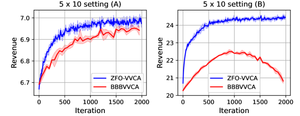
Figure 1: Training curves for ZFO-VVCA and BBBVVCA under $5\times 10$(A) and $5\times 10$(B). The plots depict the average results across $5$ runs, along with the $95\%$ confidence interval.

Comparison with Randomized Baselines

Both Lottery AMA and AMenuNet predefine a candidate size, denoted as $s$, and also make these $s$ candidate allocations learnable. This approach results in $O(snm)$ learnable parameters. Ideally, to maximize performance, $s$ could be set arbitrarily large. However, in practical scenarios, the size of $s$ is constrained by available computational resources. To balance performance with computational feasibility, we set $s$ to values within the set $\{32,128,1024,4096\}$ for both Lottery AMA and AMenuNet.

Under this configuration, as evidenced in Table 2(a), Lottery AMA and AMenuNet demonstrate commendable performance in smaller settings. However, in larger settings, as shown in Table 2(b), ZFO-VVCA consistently outperforms these two randomized AMA methods. This outcome suggests that, within the bounds of computational resource limitations, ZFO-VVCA is more efficient than Lottery AMA and AMenuNet, particularly in handling larger settings.

5.3 Case Study

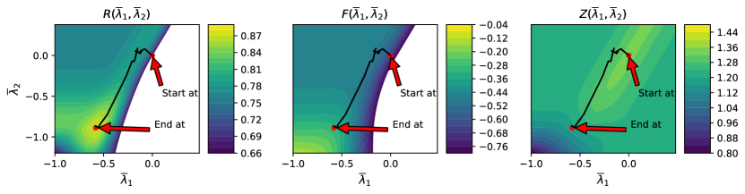
Figure 2: Training dynamics of ZFO-VVCA over $2000$ iterations in $2\times 2$(A). The parameters are set as $\lambda_{1}(\{1\})=\lambda_{2}(\{1\})=\lambda_{1}(\{2\})=\lambda_{2}(\{2\})=\bar{\lambda}_{1}\in\mathbb{R}$, $\lambda_{1}(\{1,2\})=\lambda_{2}(\{1,2\})=\bar{\lambda}_{2}\in\mathbb{R}$, $w_{1}=w_{2}=1$, and $\lambda_{1}(\emptyset)=\lambda_{2}(\emptyset)=0$. The trajectory of $(\bar{\lambda}_{1},\bar{\lambda}_{2})$ is simultaneously plotted on $R(\bar{\lambda}_{1},\bar{\lambda}_{2})$, $F(\bar{\lambda}_{1},\bar{\lambda}_{2})$, and $Z(\bar{\lambda}_{1},\bar{\lambda}_{2})$. The trajectory converges at a point balancing the values of both $F(\bar{\lambda}_{1},\bar{\lambda}_{2})$ and $Z(\bar{\lambda}_{1},\bar{\lambda}_{2})$, illustrating the effectiveness of optimizing $Z(\bar{\lambda}_{1},\bar{\lambda}_{2})$ through zeroth-order optimization.

Visualization of the Training Process

To visualize the training process of ZFO-VVCA, we adopt a symmetric simplification for bidders and items in $2\times 2$(A). Specifically, we fix the bidder weights $w_{1}=w_{2}=1$ and set bidder boost variables as follows: $\lambda_{1}(\emptyset)=\lambda_{2}(\emptyset)=0$, $\lambda_{1}(\{1\})=\lambda_{2}(\{1\})=\lambda_{1}(\{2\})=\lambda_{2}(\{2\})=\bar{\lambda}_{1}$, and $\lambda_{1}(\{1,2\})=\lambda_{2}(\{1,2\})=\bar{\lambda}_{2}$. Under this simplification, when fixing a dataset of valuation $\mathcal{S}$, we use $R(\bar{\lambda}_{1},\bar{\lambda}_{2})$, $F(\bar{\lambda}_{1},\bar{\lambda}_{2})$, and $Z(\bar{\lambda}_{1},\bar{\lambda}_{2})$ to denote $R_{\mathcal{S}}({\bm{w}},\bm{\lambda})$, $F_{\mathcal{S}}({\bm{w}},\bm{\lambda})$, $Z_{\mathcal{S}}({\bm{w}},\bm{\lambda})$, respectively.

In Figure 2, we illustrate the trajectory of $(\bar{\lambda}_{1},\bar{\lambda}_{2})$ concurrently on $R(\bar{\lambda}_{1},\bar{\lambda}_{2})$, $F(\bar{\lambda}_{1},\bar{\lambda}_{2})$, and $Z(\bar{\lambda}_{1},\bar{\lambda}_{2})$. Here, $R(\bar{\lambda}_{1},\bar{\lambda}_{2})=F(\bar{\lambda}_{1},\bar{\lambda}_{2})+Z(\bar{\lambda}_{1},\bar{\lambda}_{2})$ according to Equation 7. The trajectory initiates from a VCG auction (i.e., $\bar{\lambda}_{1}=\bar{\lambda}_{2}=0$), and converges to an improved solution that balances the values of both $F(\bar{\lambda}_{1},\bar{\lambda}_{2})$ and $Z(\bar{\lambda}_{1},\bar{\lambda}_{2})$. This outcome underscores the efficacy of our zeroth-order optimization to optimize $Z(\bar{\lambda}_{1},\bar{\lambda}_{2})$.

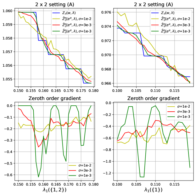
Figure 3: Visualization of $Z_{\mathcal{S}}(e^{\bm{\alpha}},{\bm{\lambda}})$, $\tilde{Z}^{\sigma}_{\mathcal{S}}(e^{\bm{\alpha}},{\bm{\lambda}})$, and the corresponding zeroth-order gradient $\tilde{\nabla}Z_{\mathcal{S}}(e^{\bm{\alpha}},{\bm{\lambda}})$ in $2\times 2$(A) with respect to one parameter. The values of $\sigma$ are chosen from the set $\{0.01,0.003,0.001\}$.

Case Study of Zeroth-Order Gradient

To further illustrate the impact of the zeroth-order method in ZFO-VVCA, we explore a $2\times 2$(A) scenario, adjusting only one of the boost variables $\lambda$ while maintaining the remaining VVCA parameters fixed. We plot $Z_{\mathcal{S}}({\bm{w}},\bm{\lambda})$ alongside the computed $\tilde{Z}^{\sigma}_{\mathcal{S}}({\bm{w}},\bm{\lambda})$ for three distinct $\sigma$ values in Figure 3. The figure shows that $Z_{\mathcal{S}}({\bm{w}},\bm{\lambda})$ experiences non-differentiability at several points, rendering first-order gradient methods infeasible. The zeroth-order method addresses this by smoothing $Z_{\mathcal{S}}({\bm{w}},\bm{\lambda})$, with varying smoothness achieved by different $\sigma$ values. Specifically, a smaller $\sigma$ provides a closer approximation of $\tilde{Z}^{\sigma}_{\mathcal{S}}({\bm{w}},\bm{\lambda})$ to $Z_{\mathcal{S}}({\bm{w}},\bm{\lambda})$. Conversely, a larger $\sigma$ results in a less precise approximation but more effectively captures the general trend with a flatter gradient. Though these insights emphasize the criticality of careful parameter selection in ZFO-VVCA, they do not necessarily imply difficulty in tuning the hyperparameters. In practice, our experiments indicate that $\sigma$ values within the range of $\{0.01,0.003,0.001\}$ are generally well-suited for most scenarios.

6 Conclusion and Future Work

In this paper, we present ZFO-VVCA, an innovative VVCA design algorithm that leverages a hybrid optimization approach, combining both zeroth-order and first-order methods. Our method employs a GPU-friendly dynamic programming algorithm to compute the winning allocation and revenue in a VVCA efficiently. Subsequently, we decompose the revenue into differentiable and non-differentiable components. The gradient of the differentiable portion is computed through standard differentiation techniques. For the non-differentiable part, we utilize a zeroth-order method to approximate the gradient of its Gaussian smoothing approximation. This results in an unbiased estimated gradient concerning an approximated objective function. Finally, experimental results showcase our proposed approach’s efficacy, stability, and scalability.

As for future work, it would be interesting to explore extending ZFO-VVCA to contextual auctions or adapting it for application in industrial scenarios.

Appendix A Omitted Proof

A.1 Proof of Theorem 4.1

See 4.1

Proof.

Clearly, the initialization loop and the final loop involve $2^{m}$ and $n$ enumerations, respectively. In the dynamic programming loop, for each bidder $i\in[2,n]$ and bundle $|\mathcal{S}|=k$, we need to enumerate all $2^{k}$ subsets of $\mathcal{S}$. Consequently, the total number of enumerations for bidder $i$ is given by $\sum_{k=0}^{m}\binom{m}{k}2^{k}=(2+1)^{m}=3^{m}.$ Since the computation during each enumeration is $O(1)$, the overall time complexity is $O(2^{m})+O((n-1)3^{m})+O(n)=O(n3^{m})$.

Regarding space complexity, apart from the $O(n2^{m})$ needed for input valuations and VVCA parameters, we require an additional $O(n2^{m})$ space to store $\mathrm{MAW}$ and $\mathrm{AB}$. Notably, there is no need to store $\mathrm{MAW}^{\prime}$. Therefore, the total space complexity is $O(n2^{m})$.

∎

A.2 Proof of Theorem 4.2

See 4.2

To prove Theorem 4.2, we first present a useful lemma:

Lemma A.1.

Let $W:\mathbb{R}^{n}\to\mathbb{R}$ be a bounded function such that $\max_{{\bm{x}}\in\mathbb{R}^{n}}|W(x)|\leq M_{W}$, and denote $\tilde{W}^{\sigma}\coloneqq\mathbb{E}_{{{\bm{u}}}\sim N(0,I_{n})}[W({\bm{x}}+\sigma{{\bm{u}}})]$ with $\sigma>0$ as the Gaussian smoothing approximation of $W$. Then $\tilde{W}^{\sigma}$ is differentiable.

Proof.

For any ${\bm{x}}=(x_{1},x_{2},\dots,x_{n})$, without loss of generality, let’s examine the differentiability of $\tilde{W}^{\sigma}({\bm{x}})$ with respect to $x_{1}$. We define ${\bm{x}}_{-1}=(x_{2},x_{3},\dots,x_{n})$, and for any ${{\bm{u}}}\in\mathbb{R}^{n}$, we denote ${{\bm{u}}}_{-1}=({u}_{1},{{\bm{u}}}_{-1})$.

Existence of $\frac{\partial\tilde{W}^{\sigma}({\bm{x}})}{\partial x_{1}}$

We prove the existence of $\frac{\partial\tilde{W}^{\sigma}({\bm{x}})}{\partial x_{1}}$ by deriving according to the definition of partial derivative:

$$\lim_{\Delta x_{1}\rightarrow 0}\frac{\tilde{W}^{\sigma}(x_{1}+\Delta x_{1},{\bm{x}}_{-1})-\tilde{W}^{\sigma}(x_{1},{\bm{x}}_{-1})}{\Delta x_{1}}$$ (10)

$$=\lim_{\Delta x_{1}\rightarrow 0}\frac{\mathbb{E}_{{{\bm{u}}}\sim N(0,I_{n})}[W(x_{1}+\Delta x_{1}+\sigma{u}_{1},{\bm{x}}_{-1}+\sigma{{\bm{u}}}_{-1})]-\mathbb{E}_{{{\bm{u}}}\sim N(0,I_{n})}[W({\bm{x}}+\sigma{{\bm{u}}})]}{\Delta x_{1}}$$

$$=\lim_{\Delta x_{1}\rightarrow 0}\frac{\mathbb{E}_{{{\bm{u}}}^{\prime}\coloneqq({u}^{\prime}_{1},{{\bm{u}}}_{-1})\sim N((\frac{\Delta x_{1}}{\sigma},\bm{0}_{n-1}),I_{n})}[W({\bm{x}}+\sigma{{\bm{u}}}^{\prime})]-\mathbb{E}_{{{\bm{u}}}\sim N(0,I_{n})}[W({\bm{x}}+\sigma{{\bm{u}}})]}{\Delta x_{1}}$$

$$=\lim_{\Delta x_{1}\rightarrow 0}\left(\frac{1}{2\pi}\right)^{\frac{n}{2}}\int W(\bm{x}+\sigma{{\bm{u}}})\frac{\exp\left(-\frac{1}{2}\|({u}_{1}-\frac{\Delta x_{1}}{\sigma},{{\bm{u}}}_{-1})\|^{2}\right)-\exp\left(-\frac{1}{2}\|({u}_{1},{{\bm{u}}}_{-1})\|^{2}\right)}{\Delta x_{1}}d{{\bm{u}}}$$

$$\overset{(a)}{=}\left(\frac{1}{2\pi}\right)^{\frac{n}{2}}\int W(\bm{x}+\sigma{{\bm{u}}})\frac{{u}_{1}}{\sigma}\exp\left(-\frac{1}{2}\|{{\bm{u}}}\|^{2}\right)d{{\bm{u}}}$$

$$=\mathbb{E}_{{{\bm{u}}}\sim N(0,I)}\left[\frac{W({\bm{x}}+\sigma{{\bm{u}}})}{\sigma}{u}_{1}\right]$$

$$=\mathbb{E}_{{{\bm{u}}}\sim N(0,I)}\left[\frac{W({\bm{x}}+\sigma{{\bm{u}}})-W({\bm{x}})}{\sigma}{u}_{1}\right],\quad\text{since }\mathbb{E}_{{{\bm{u}}}\sim N(0,I)}[W({\bm{x}}){u}_{1}]=0,$$

where $(a)$ in Equation 10 essentially comes from Taylor expansion. To provide its proof in detail, we first define $f(t)\coloneqq\exp\left(-\frac{1}{2}\|(t,{{\bm{u}}}_{-1})\|^{2}\right)$. Then we use Taylor expansion of $f({u}_{1}-\frac{\Delta x_{1}}{\sigma})$ at ${u}_{1}$ with Lagrange remainder, that is,

$$f({u}_{1}-\frac{\Delta x_{1}}{\sigma})=f({u}_{1})+f^{\prime}({u}_{1})(-\frac{\Delta x_{1}}{\sigma})+f^{\prime\prime}(\xi(\Delta x_{1},u_{1}))\frac{(\Delta x_{1})^{2}}{\sigma^{2}}$$

$$= f({u}_{1})+{u}_{1}\exp\left(-\frac{1}{2}\|({u}_{1},{{\bm{u}}}_{-1})\|^{2}\right)\frac{\Delta x_{1}}{\sigma}+(\xi^{2}(\Delta x_{1},u_{1})-1)\exp\left(-\frac{1}{2}\|(\xi(\Delta x_{1},u_{1}),{{\bm{u}}}_{-1})\|^{2}\right)\frac{(\Delta x_{1})^{2}}{\sigma^{2}}$$

where $\xi(\Delta x_{1},u_{1})$ is between $u_{1}-\frac{\Delta x_{1}}{\sigma}$ and $u_{1}$. On top of that, $(a)$ is derived by

$$\lim_{\Delta x_{1}\rightarrow 0}\int W(\bm{x}+\sigma{{\bm{u}}})\frac{\exp\left(-\frac{1}{2}\|({u}_{1}-\frac{\Delta x_{1}}{\sigma},{{\bm{u}}}_{-1})\|^{2}\right)-\exp\left(-\frac{1}{2}\|({u}_{1},{{\bm{u}}}_{-1})\|^{2}\right)}{\Delta x_{1}}d{{\bm{u}}}$$ (11)

$$= \lim_{\Delta x_{1}\rightarrow 0}\int W(\bm{x}+\sigma{{\bm{u}}})\frac{{u}_{1}\exp\left(-\frac{1}{2}\|({u}_{1},{{\bm{u}}}_{-1})\|^{2}\right)\frac{\Delta x_{1}}{\sigma}+(\xi^{2}(\Delta x_{1},u_{1})-1)\exp\left(-\frac{1}{2}\|(\xi(\Delta x_{1},u_{1}),{{\bm{u}}}_{-1})\|^{2}\right)\frac{(\Delta x_{1})^{2}}{\sigma^{2}}}{\Delta x_{1}}d{{\bm{u}}}$$

$$= \lim_{\Delta x_{1}\rightarrow 0}\int W(\bm{x}+\sigma{{\bm{u}}})\left(\frac{{u}_{1}}{\sigma}\exp\left(-\frac{1}{2}\|{{\bm{u}}}\|^{2}\right)+(\xi^{2}(\Delta x_{1},u_{1})-1)\exp\left(-\frac{1}{2}\|(\xi(\Delta x_{1},u_{1}),{{\bm{u}}}_{-1})\|^{2}\right)\frac{\Delta x_{1}}{\sigma^{2}}\right)d{{\bm{u}}}$$

$$\overset{(b)}{=} \lim_{\Delta x_{1}\rightarrow 0}\int W(\bm{x}+\sigma{{\bm{u}}})\frac{{u}_{1}}{\sigma}\exp\left(-\frac{1}{2}\|{{\bm{u}}}\|^{2}\right)d{{\bm{u}}}$$

$$= \int W(\bm{x}+\sigma{{\bm{u}}})\frac{{u}_{1}}{\sigma}\exp\left(-\frac{1}{2}\|{{\bm{u}}}\|^{2}\right)d{{\bm{u}}},$$

where $(b)$ is equivalent to the truth of the following equation:

$$\lim_{\Delta x_{1}\to 0}\left|\Delta x_{1}\int W(x+\sigma{{\bm{u}}})(\xi^{2}(\Delta x_{1},u_{1})-1)\exp\left(-\frac{1}{2}\|(\xi(\Delta x_{1},u_{1}),{{\bm{u}}}_{-1})\|^{2}\right)d{{\bm{u}}}\right|$$ (12)

$$\leq \lim_{\Delta x_{1}\to 0}|\Delta x_{1}|\cdot\Big{|}W(x+\sigma{{\bm{u}}})\Big{|}\cdot\left|\int(\xi^{2}(\Delta x_{1},u_{1})-1)\exp\left(-\frac{1}{2}\|(\xi(\Delta x_{1},u_{1}),{{\bm{u}}}_{-1})\|^{2}\right)d{{\bm{u}}}\right|$$

$$\leq \lim_{\Delta x_{1}\to 0}|\Delta x_{1}|\cdot M_{W}\cdot\left|\int(\xi^{2}(\Delta x_{1},u_{1})-1)\exp\left(-\frac{1}{2}\|(\xi(\Delta x_{1},u_{1}),{{\bm{u}}}_{-1})\|^{2}\right)d{{\bm{u}}}\right|$$

$$= \lim_{\Delta x_{1}\to 0}|\Delta x_{1}|\cdot M_{W}\cdot\left|\int K(\xi(\Delta x_{1},u_{1}),{{\bm{u}}}_{-1})d{{\bm{u}}}\right|$$

$$\leq \lim_{\Delta x_{1}\to 0}|\Delta x_{1}|\cdot M_{W}\cdot\int\Big{|}K(\xi(\Delta x_{1},u_{1}),{{\bm{u}}}_{-1})\Big{|}d{{\bm{u}}}$$

where we define $K(s,{{\bm{u}}}_{-1})\coloneqq(s^{2}-1)\exp\left(-\frac{1}{2}\|(s,{{\bm{u}}}_{-1})\|^{2}\right)$ with $|s-u_{1}|\leq\left|\frac{\Delta x_{1}}{\sigma}\right|$, and we prove $(c)$ by showing that when $|\Delta x_{1}|<\sigma$, the term

$$\int\Big{|}K(\xi(\Delta x_{1},u_{1}),{{\bm{u}}}_{-1})\Big{|}d{{\bm{u}}}\leq\int\max_{s\in[u_{1}-|\frac{\Delta x_{1}}{\sigma}|,u_{1}+|\frac{\Delta x_{1}}{\sigma}|]}|K(s,{{\bm{u}}}_{-1})|d{{\bm{u}}}$$ (13)

is bounded: Given the definition of $K$, there exists a constant $C_{K}>1$ such that when $s>C_{K}$, $|K(s,{{\bm{u}}}_{-1})|$ is monotone decreasing with respect to $s$, and when $s<-C_{K}$, $|K(s,{{\bm{u}}}_{-1})|$ is monotone increasing with respect to $s$. Based on that, we discuss the following three cases of the range of $u_{1}$:

1. When $u_{1}>2C_{k}$, then $s\geq u-\left|\frac{\Delta x_{1}}{\sigma}\right|>2C_{K}-1>C_{K}$, so that $|K(s,{{\bm{u}}}_{-1})|$ is monotone decreasing with respect to $s$. Therefore we have

   $$\int\limits_{u_{1}>2C_{K}}\max_{s\in[u_{1}-|\frac{\Delta x_{1}}{\sigma}|,u_{1}+|\frac{\Delta x_{1}}{\sigma}|]}\Big{|}K(s,{{\bm{u}}}_{-1})\Big{|}d{{\bm{u}}}\leq\int\limits_{u_{1}>2C_{K}}\left|K(u_{1}-\left|\frac{\Delta x_{1}}{\sigma}\right|,{{\bm{u}}}_{-1})\right|d{{\bm{u}}}$$

   $$\leq \int\limits_{u_{1}>2C_{K}}\Big{|}K(u_{1}-1,{{\bm{u}}}_{-1})\Big{|}d{{\bm{u}}}=:C_{1},$$

   where $C_{1}$ is a constant independent of $|\Delta x_{1}|$.

2. When $-2C_{K}\leq u_{1}\leq 2C_{K}$, we have

   $$\int\limits_{-2C_{K}\leq u_{1}\leq 2C_{K}}\max_{s\in[u_{1}-|\frac{\Delta x_{1}}{\sigma}|,u_{1}+|\frac{\Delta x_{1}}{\sigma}|]}\Big{|}K(s,{{\bm{u}}}_{-1})\Big{|}d{{\bm{u}}}$$

   $$\leq \int\limits_{-2C_{K}\leq u_{1}\leq 2C_{K}}\max_{-2C_{K}\leq u^{\prime}_{1}\leq 2C_{K}}\left(\max_{s\in[u^{\prime}_{1}-|\frac{\Delta x_{1}}{\sigma}|,u^{\prime}_{1}+|\frac{\Delta x_{1}}{\sigma}|]}\Big{|}K(s,{{\bm{u}}}_{-1})\Big{|}\right)d{{\bm{u}}}$$

   $$\leq \int\limits_{-2C_{K}\leq u_{1}\leq 2C_{K}}\max_{-(2C_{K}+1)\leq s\leq(2C_{K}+1)}\Big{|}K(s,{{\bm{u}}}_{-1})\Big{|}d{{\bm{u}}}=:C_{2}$$

   where $C_{2}$ is a constant independent of $|\Delta x_{1}|$.

3. When $u_{1}<-2C_{K}$, then $s\leq u+\left|\frac{\Delta x_{1}}{\sigma}\right|<-2C_{K}+1<C_{K}$, so that $|K(s,{{\bm{u}}}_{-1})|$ is monotone increasing with respect to $s$. Similar to case 1, we have

   $$\int\limits_{u_{1}<-2C_{K}}\max_{s\in[u_{1}-|\frac{\Delta x_{1}}{\sigma}|,u_{1}+|\frac{\Delta x_{1}}{\sigma}|]}\Big{|}K(s,{{\bm{u}}}_{-1})\Big{|}d{{\bm{u}}}\leq\int\limits_{u_{1}<-2C_{K}}\left|K(u_{1}+\left|\frac{\Delta x_{1}}{\sigma}\right|,{{\bm{u}}}_{-1})\right|d{{\bm{u}}}$$

   $$\leq \int\limits_{u_{1}<-2C_{K}}\Big{|}K(u_{1}+1,{{\bm{u}}}_{-1})\Big{|}d{{\bm{u}}}=:C_{3}$$

   where $C_{3}$ is a constant independent of $|\Delta x_{1}|$.

Therefore, Equation 13 is bounded by $C_{1}+C_{2}+C_{3}$ which is independent of $|\Delta x_{1}|$, and the proof of Equation 12 is complete. Subsequently, the proof of $(b)$ in Equation 11 is established. Following that, the proof of $(a)$ in Equation 10 is concluded. Consequently, the existence of $\frac{\partial\tilde{W}^{\sigma}({\bm{x}})}{\partial x_{1}}$ is derived from Equation 10.

Continuity of $\frac{\partial\tilde{W}^{\sigma}({\bm{x}})}{\partial x_{1}}$

Given $\sigma$, let $Q(\bm{x})\coloneqq W(\frac{\bm{x}}{\sigma})$ and $H({{\bm{u}}})\coloneqq-{u}_{1}\exp\left(-\frac{1}{2}\left\|{{\bm{u}}}\right\|^{2}\right)$, according to Equation 10 we have

$$\frac{\partial\tilde{W}^{\sigma}({\bm{x}})}{\partial x_{1}} =\frac{1}{\sigma}\left(\frac{1}{2\pi}\right)^{\frac{n}{2}}\int W(\bm{x}+\sigma{{\bm{u}}}){u}_{1}\exp\left(-\frac{1}{2}\|{{\bm{u}}}\|^{2}\right)d{{\bm{u}}}$$

$$=\frac{1}{\sigma}\left(\frac{1}{2\pi}\right)^{\frac{n}{2}}\int Q({{\bm{u}}}+\frac{\bm{x}}{\sigma})H(-{{\bm{u}}})d{{\bm{u}}}$$

$$=\frac{1}{\sigma}\left(\frac{1}{2\pi}\right)^{\frac{n}{2}}\int Q({{\bm{u}}})H(\frac{\bm{x}}{\sigma}-{{\bm{u}}})d{{\bm{u}}}$$

$$=:\frac{1}{\sigma}\left(\frac{1}{2\pi}\right)^{\frac{n}{2}}C(\frac{{\bm{x}}}{\sigma}),$$

where we can see that $C(\frac{{\bm{x}}}{\sigma})$ is a convolution function. As for the continuity of $C(\frac{{\bm{x}}}{\sigma})$, we have:

$$\lim_{\bm{h}\rightarrow 0}\left|C(\frac{\bm{x}}{\sigma}+\bm{h})-C(\frac{\bm{x}}{\sigma})\right| =\lim_{\bm{h}\rightarrow 0}\left|\int H(\frac{\bm{x}}{\sigma}+\bm{h}-{{\bm{u}}})Q({{\bm{u}}})d{{\bm{u}}}-\int H(\frac{\bm{x}}{\sigma}-{{\bm{u}}})Q({{\bm{u}}})d{{\bm{u}}}\right|$$

$$\leq\lim_{\bm{h}\rightarrow 0}\int\left|H(\frac{\bm{x}}{\sigma}+\bm{h}-{{\bm{u}}})-H(\frac{\bm{x}}{\sigma}-{{\bm{u}}})\right|\left|Q({{\bm{u}}})\right|d{{\bm{u}}}$$

$$\overset{(a)}{\leq}\lim_{\bm{h}\rightarrow 0}M_{W}\int\left|H(\frac{\bm{x}}{\sigma}+\bm{h}-{{\bm{u}}})-H(\frac{\bm{x}}{\sigma}-{{\bm{u}}})\right|d{{\bm{u}}}$$

$$\overset{(b)}{=}0,$$

where $(a)$ holds because $Q_{\sigma}(\bm{x})\coloneqq W(\frac{\bm{x}}{\sigma})$ is bounded by $M_{W}\coloneqq\max_{\bm{x}}W({\bm{x}})$, and $(b)$ holds because $H({{\bm{u}}})$ is integrable. As a result, $C(\frac{{\bm{x}}}{\sigma})$ is continuous with respect to ${\bm{x}}$, and then $\frac{\partial\tilde{W}^{\sigma}({\bm{x}})}{\partial x_{1}}$ is also continuous with respect to $x_{1}$.

Differentiability of $\tilde{W}^{\sigma}$

From the preceding discussion, it is evident that $\tilde{W}^{\sigma}({\bm{x}})$ is differentiable with respect to $x_{1}$. This technique can be extended straightforwardly to $x_{2},x_{3},\dots,x_{n}$. Therefore, $\tilde{W}^{\sigma}({\bm{x}})$ is differentiable (and thus continuous) with respect to ${\bm{x}}$.

∎

Proof of Theorem 4.2.

$\tilde{Z}_{\mathcal{S}}^{\sigma}(e^{\bm{\alpha}},\bm{\lambda})$ is defined as the Gaussian smoothing approximation of ${Z}_{\mathcal{S}}(e^{\bm{\alpha}},\bm{\lambda})$, whose range is $[\min_{V\in\mathcal{S}}\min_{A\in\mathcal{A}}\sum_{i=1}^{n}v_{i}(A),\max_{V\in\mathcal{S}}\max_{A\in\mathcal{A}}\sum_{i=1}^{n}v_{i}(A)]$. Therefore, the proof is done by applying Lemma A.1.

∎

Appendix B Further Implementation Details

Table 2: Hyperparameters of Lottery AMA Curry et al. [2023] and AMenuNet Duan et al. [2023] in different settings.

Candidate Size	Symmetric			Asymmetric
	2$\times$2 (A)	2$\times$2 (D)	2$\times$5 (A)	2$\times$5 (C)	5$\times$3 (C)	5$\times$3 (B)
Lottery AMA	32	32	128	128	128	128
AMenuNet	32	32	128	128	128	128
Candidate Size	Symmetric			Asymmetric
	3$\times$10 (A)	3$\times$10 (D)	5$\times$10 (A)	3$\times$10 (B)	5$\times$10 (B)	5$\times$10 (C)
Lottery AMA	1024	1024	4096	1024	4096	4096
AMenuNet	1024	1024	4096	1024	4096	4096

Lottery AMA Curry et al. [2023] and AMenuNet Duan et al. [2023]

For all the settings in our experiments, we set the same hyperparameters as in the original paper except for the candidate size. And we adjust the candidate size according to the complexity of the auction scenario, which is shown in Table 2.

Table 3: Hyperparameters of ZFO-VVCA and the ablation version FO-VVCA in different settings.

	Symmetric			Asymmetric
	2$\times$2 (A)	2$\times$2 (D)	2$\times$5 (A)	2$\times$5 (C)	5$\times$3 (C)	5$\times$3 (B)
Learning Rate	0.01	0.01	0.001	0.001	0.001	0.001
Number of Random Directions $n_{r}$	8	8	8	8	8	8
Standard Deviation $\sigma$	0.01	0.01	0.01	0.01	0.01	0.01
Training Iteration	2000	2000	2000	2000	2000	2000
Batch Size	1024	1024	2048	2048	1024	1024
	Symmetric			Asymmetric
	3$\times$10 (A)	3$\times$10 (D)	5$\times$10 (A)	3$\times$10 (B)	5$\times$10 (B)	5$\times$10 (C)
Learning Rate	0.001	0.001	0.0003	0.01	0.005	0.005
Number of Random Directions $n_{r}$	8	8	8	8	8	8
Standard Deviation $\sigma$	0.01	0.01	0.001	0.01	0.01	0.01
Training Iteration	2000	2000	2000	2000	2000	2000
Batch Size	1024	1024	1024	1024	1024	1024

ZFO-VVCA (Ours) and the Ablation Version FO-VVCA

We list the main hyperparameters used in our experiments in Table 3.

References

• Balasubramanian and Ghadimi [2018] Krishnakumar Balasubramanian and Saeed Ghadimi. Zeroth-order (non)-convex stochastic optimization via conditional gradient and gradient updates. Advances in Neural Information Processing Systems, 31, 2018.
• Balcan et al. [2021] M-F Balcan, Siddharth Prasad, and Tuomas Sandholm. Learning within an instance for designing high-revenue combinatorial auctions. In IJCAI Annual Conference, 2021.
• Balcan et al. [2018] Maria-Florina Balcan, Tuomas Sandholm, and Ellen Vitercik. A general theory of sample complexity for multi-item profit maximization. In Proceedings of the 2018 ACM Conference on Economics and Computation, pages 173–174, 2018.
• Balcan et al. [2023] Maria-Florina Balcan, Tuomas Sandholm, and Ellen Vitercik. Generalization guarantees for multi-item profit maximization: Pricing, auctions, and randomized mechanisms. Operations Research, 2023.
• Balcan et al. [2016] Maria-Florina F Balcan, Tuomas Sandholm, and Ellen Vitercik. Sample complexity of automated mechanism design. Advances in Neural Information Processing Systems, 29, 2016.
• Bichler et al. [2021] Martin Bichler, Maximilian Fichtl, Stefan Heidekrüger, Nils Kohring, and Paul Sutterer. Learning equilibria in symmetric auction games using artificial neural networks. Nature machine intelligence, 3(8):687–695, 2021.
• Chen et al. [2019] Xiangyi Chen, Sijia Liu, Kaidi Xu, Xingguo Li, Xue Lin, Mingyi Hong, and David Cox. Zo-adamm: Zeroth-order adaptive momentum method for black-box optimization. Advances in neural information processing systems, 32, 2019.
• Curry et al. [2020] Michael Curry, Ping-Yeh Chiang, Tom Goldstein, and John Dickerson. Certifying strategyproof auction networks. Advances in Neural Information Processing Systems, 33:4987–4998, 2020.
• Curry et al. [2022] Michael J Curry, Uro Lyi, Tom Goldstein, and John P Dickerson. Learning revenue-maximizing auctions with differentiable matching. In International Conference on Artificial Intelligence and Statistics, pages 6062–6073. PMLR, 2022.
• Curry et al. [2023] Michael J. Curry, Tuomas Sandholm, and John P. Dickerson. Differentiable economics for randomized affine maximizer auctions. In Proceedings of the Thirty-Second International Joint Conference on Artificial Intelligence, IJCAI 2023, 19th-25th August 2023, Macao, SAR, China, pages 2633–2641. ijcai.org, 2023. doi: 10.24963/ijcai.2023/293. URL https://doi.org/10.24963/ijcai.2023/293.
• Duan et al. [2022] Zhijian Duan, Jingwu Tang, Yutong Yin, Zhe Feng, Xiang Yan, Manzil Zaheer, and Xiaotie Deng. A context-integrated transformer-based neural network for auction design. In International Conference on Machine Learning, pages 5609–5626. PMLR, 2022.
• Duan et al. [2023] Zhijian Duan, Haoran Sun, Yurong Chen, and Xiaotie Deng. A scalable neural network for DSIC affine maximizer auction design. arXiv preprint arXiv:2305.12162, 2023.
• Duchi et al. [2015] John C Duchi, Michael I Jordan, Martin J Wainwright, and Andre Wibisono. Optimal rates for zero-order convex optimization: The power of two function evaluations. IEEE Transactions on Information Theory, 61(5):2788–2806, 2015.
• Dütting et al. [2019] Paul Dütting, Zhe Feng, Harikrishna Narasimhan, David Parkes, and Sai Srivatsa Ravindranath. Optimal auctions through deep learning. In International Conference on Machine Learning, pages 1706–1715. PMLR, 2019.
• Dütting et al. [2023] Paul Dütting, Zhe Feng, Harikrishna Narasimhan, David C Parkes, and Sai Srivatsa Ravindranath. Optimal auctions through deep learning: Advances in differentiable economics. Journal of the ACM, 2023.
• Flaxman et al. [2004] Abraham D Flaxman, Adam Tauman Kalai, and H Brendan McMahan. Online convex optimization in the bandit setting: gradient descent without a gradient. arXiv preprint cs/0408007, 2004.
• Ghadimi et al. [2016] Saeed Ghadimi, Guanghui Lan, and Hongchao Zhang. Mini-batch stochastic approximation methods for nonconvex stochastic composite optimization. Mathematical Programming, 155(1-2):267–305, 2016.
• Golowich et al. [2018] Noah Golowich, Harikrishna Narasimhan, and David C Parkes. Deep learning for multi-facility location mechanism design. In IJCAI, pages 261–267, 2018.
• Ivanov et al. [2022] Dmitry Ivanov, Iskander Safiulin, Igor Filippov, and Ksenia Balabaeva. Optimal-er auctions through attention. Advances in Neural Information Processing Systems, 35:34734–34747, 2022.
• Jehiel et al. [2007] Philippe Jehiel, Moritz Meyer-Ter-Vehn, and Benny Moldovanu. Mixed bundling auctions. Journal of Economic Theory, 134(1):494–512, 2007.
• Lavi et al. [2003] Ron Lavi, Ahuva Mu’Alem, and Noam Nisan. Towards a characterization of truthful combinatorial auctions. In 44th Annual IEEE Symposium on Foundations of Computer Science, 2003. Proceedings., pages 574–583. IEEE, 2003.
• Li et al. [2024] Xuejian Li, Ze Wang, Bingqi Zhu, Fei He, Yongkang Wang, and Xingxing Wang. Deep automated mechanism design for integrating ad auction and allocation in feed. arXiv preprint arXiv:2401.01656, 2024.
• Likhodedov and Sandholm [2004] Anton Likhodedov and Tuomas Sandholm. Methods for boosting revenue in combinatorial auctions. In AAAI, pages 232–237, 2004.
• Likhodedov et al. [2005] Anton Likhodedov, Tuomas Sandholm, et al. Approximating revenue-maximizing combinatorial auctions. In AAAI, volume 5, pages 267–274, 2005.
• Liu et al. [2018] Sijia Liu, Jie Chen, Pin-Yu Chen, and Alfred Hero. Zeroth-order online alternating direction method of multipliers: Convergence analysis and applications. In International Conference on Artificial Intelligence and Statistics, pages 288–297. PMLR, 2018.
• Liu et al. [2020] Sijia Liu, Songtao Lu, Xiangyi Chen, Yao Feng, Kaidi Xu, Abdullah Al-Dujaili, Mingyi Hong, and Una-May O’Reilly. Min-max optimization without gradients: Convergence and applications to black-box evasion and poisoning attacks. In International conference on machine learning, pages 6282–6293. PMLR, 2020.
• Myerson [1981] Roger B Myerson. Optimal auction design. Mathematics of operations research, 6(1):58–73, 1981.
• Nesterov and Spokoiny [2017] Yurii Nesterov and Vladimir Spokoiny. Random gradient-free minimization of convex functions. Foundations of Computational Mathematics, 17:527–566, 2017.
• Peri et al. [2021] Neehar Peri, Michael Curry, Samuel Dooley, and John Dickerson. Preferencenet: Encoding human preferences in auction design with deep learning. Advances in Neural Information Processing Systems, 34:17532–17542, 2021.
• Rahme et al. [2021a] Jad Rahme, Samy Jelassi, Joan Bruna, and S Matthew Weinberg. A permutation-equivariant neural network architecture for auction design. In Proceedings of the AAAI Conference on Artificial Intelligence, volume 35, pages 5664–5672, 2021a.
• Rahme et al. [2021b] Jad Rahme, Samy Jelassi, and S. Matthew Weinberg. Auction learning as a two-player game. In International Conference on Learning Representations, 2021b. URL https://openreview.net/forum?id=YHdeAO61l6T.
• Rao [2019] Singiresu S Rao. Engineering optimization: theory and practice. John Wiley & Sons, 2019.
• Ravindranath et al. [2021] Sai Srivatsa Ravindranath, Zhe Feng, Shira Li, Jonathan Ma, Scott D Kominers, and David C Parkes. Deep learning for two-sided matching. arXiv preprint arXiv:2107.03427, 2021.
• Ravindranath et al. [2023] Sai Srivatsa Ravindranath, Yanchen Jiang, and David C. Parkes. Data market design through deep learning. In Thirty-seventh Conference on Neural Information Processing Systems, 2023. URL https://openreview.net/forum?id=sgCrNMOuXp.
• Roberts [1979] Kevin Roberts. The characterization of implementable choice rules. Aggregation and revelation of preferences, 12(2):321–348, 1979.
• Salimans et al. [2017] Tim Salimans, Jonathan Ho, Xi Chen, Szymon Sidor, and Ilya Sutskever. Evolution strategies as a scalable alternative to reinforcement learning. arXiv preprint arXiv:1703.03864, 2017.
• Sandholm and Likhodedov [2015] Tuomas Sandholm and Anton Likhodedov. Automated design of revenue-maximizing combinatorial auctions. Operations Research, 63(5):1000–1025, 2015.
• Spall [2005] James C Spall. Introduction to stochastic search and optimization: estimation, simulation, and control. John Wiley & Sons, 2005.
• Tang and Sandholm [2012] Pingzhong Tang and Tuomas Sandholm. Mixed-bundling auctions with reserve prices. In AAMAS, pages 729–736, 2012.
• Vickrey [1961] William Vickrey. Counterspeculation, auctions, and competitive sealed tenders. The Journal of finance, 16(1):8–37, 1961.