SoLA: Solver-Layer Adaption of LLM for Better Logic Reasoning

Abstract

Considering the challenges faced by large language models (LLMs) on logical reasoning, prior efforts have sought to transform problem-solving through tool learning. While progress has been made on small-scale problems, solving industrial cases remains difficult due to their large scale and intricate expressions. In this paper, we propose a novel solver-layer adaptation (SoLA) method, where we introduce a solver as a new layer of the LLM to differentially guide solutions towards satisfiability. In SoLA, LLM aims to comprehend the search space described in natural language and identify local solutions of the highest quality, while the solver layer focuses solely on constraints not satisfied by the initial solution. Leveraging MaxSAT as a bridge, we define forward and backward transfer gradients, enabling the final model to converge to a satisfied solution or prove unsatisfiability. The backdoor theory ensures that SoLA can obtain accurate solutions within polynomial loops. We evaluate the performance of SoLA on various datasets and empirically demonstrate its consistent outperformance against existing symbolic solvers (including Z3 and Kissat) and tool-learning methods in terms of efficiency in large-scale problem-solving.

1 Introduction

Logical reasoning plays a crucial role in tasks such as problem-solving and decision-making, enabling humans to structure knowledge, analyze relationships between vast amounts of information, and draw inferences based on logical rules and constraints. Numerous efforts have been undertaken to enhance the ability of Large Language Models (LLMs) in logical reasoning. These include approaches like text-based temporal reasoning (Xiong et al., 2024), logic feedback-enhanced alignment methods (Nguyen et al., 2023), and prompt-based methods such as the chain of thoughts, tree of thoughts, or a simple directive like ”Let’s think step by step” (Lightman, 2023). To further bolster the reasoning ability of LLMs, an AlphaZero-like tree-search learning framework has been introduced. This framework demonstrates how tree-search, coupled with a learned value function, can guide LLMs’ decoding and enhance their reasoning abilities (Feng et al., 2023b). Despite the strides made by LLMs in achieving human-like reasoning abilities, they still encounter challenges when confronted with complex logical reasoning problems. Occasionally, LLMs exhibit unfaithful reasoning, leading to derived conclusions that do not consistently follow the previously generated reasoning chain in practical applications (Pan et al., 2023).

To this end, recent works have begun to augment LLMs with access to external solvers, i.e., utilize LLMs to first parse natural language logical questions into symbolic representations and subsequently employ external solvers to generate answers based on these representations. To enhance parsing accuracy, LoGiPT (Feng et al., 2023a) has been proposed to directly emulate the reasoning processes and mitigate the parsing errors by learning to strict adherence to solver syntax and grammar. It is fine-tuned on a constructed instruction-tuning dataset derived from revealing and refining the invisible reasoning process of deductive solvers. An alternative approach for improving reasoning capabilities involves a new satisfiability-aided modeling approach (Ye X, 2023), in which an LLM is used to generate a declarative task specification and leverage an off-the-shelf automated theorem prover to derive the final answer. This method has demonstrated superiority over program-aided Language Models (LMs) by achieving a $23\%$ improvement on the GSM arithmetic reasoning dataset, establishing a new state-of-the-art.

Despite their impressive performance on various benchmark tests, two apparent disadvantages emerge, unfortunately. (i) Any parsing errors inevitably lead to the failure of the external logic solver, resulting in the inability to obtain correct answers, particularly when dealing with emerging scales and complexities. (ii) The performance of LLMs is constrained by the capabilities of the augmented solver, as LLMs exclusively handle the translation from natural language descriptions to symbolic expressions. Notably, even the state-of-the-art symbolic solvers, such as Z3 and Kissat, encounter significant bottlenecks when addressing industrial problems involving arithmetic circuit modules, for instance, high bit-width multipliers and hybrid multiply-add circuits(Shi et al., 2022a).

In this paper, we propose a new solver-layer adaption (SoLA) method, which aims to improve LLM’s logical reasoning capabilities in a novel way. Hereby, we still utilize the LLM to parse the natural language description of logic problems, and the solver is relaxed and differentiated into a new layer of LLM. After defining the forward and backward passing gradients, the differential solver layer can be utilized to get the LLM’s outputs’ refinements.

In this paper, we introduce a novel method called solver-layer adaptation (SoLA), aiming to enhance LLM’s logical reasoning capabilities. In this approach, we continue to leverage the LLM for parsing natural language descriptions of logical problems. However, the solver is relaxed, differentiated, and integrated as a new layer within the LLM. By defining forward and backward passing gradients, this differential solver layer is employed to refine the outputs of the LLM, thereby improving the logical reasoning capabilities of the LLM.

To be specific, our contributions are summarized as follows:

• It is the first work that bridges the gap between LLM’s understanding of natural language and the solver’s method based on symbolic computation, thereby enhancing end-to-end performance through the synergistic combination of the respective strengths of LLM and solvers.

• It is the first work to achieve polynomial time complexity for solving UNSAT instances. This breakthrough implies that challenging industrial UNSAT cases, typically beyond the capability of state-of-the-art solvers within several weeks, can now be inferred to be UNSAT within a relatively limited time frame.

• Compared with other learning-aided SAT solving methods, SoLA first makes use of LLM to comprehend symbolic expressions, rather than graph neural networks.

We assess the performance of our approach on both small SAT and UNSAT instances as well as challenging industrial cases. Our analysis reveals that when addressing standard instances with up to $200$ variables, SoLA substantially enhances the inference accuracy of LLM to $100\%$. Additionally, in handling large circuit cases, SoLA outperforms state-of-the-art solvers, demonstrating remarkable efficiency.

2 Related Works

In general, a CNF formula $\phi$ consists of a conjunction of clauses $\omega$, each of which denotes a disjunction of literals. A literal is either a variable $v_{i}$ or its complement. Each variable can be assigned a logic value, either $0$ or $1$. Any general Boolean problems can be represented as a CNF formula model. An SAT solver either finds an assignment such that $\phi$ is satisfied or proves that no such assignment exists, i.e., UNSAT. Modern SAT solvers are based on the conflict-driven-clause-learning (CDCL) algorithm, and it works as a basic engine for many applications. Considering the combination of machine learning and SAT, there exist two research lines.

One is to utilize learning-driven methods to improve SAT-solving efficiency, which begins at a graph neural network (GNN) to get the embedding vector and ends with a classifier (Selsam et al., 2018). This framework has been integrated with the CDCL framework as a plug-in component (Kurin et al., 2020; Zhang et al., 2020; Li et al., 2022; Shi et al., 2022a, b). Nevertheless, this pipeline suffers from two aspects: (1) Similar structures will result in similar search spaces, because of which GNN is to obtain the structural information of the problem. However, corner cases from logic equivalence checking (LEC) demonstrate that even a slight difference of less than 1% in structure can lead to thousands of times discrepancies in solving efficiency (Zhang et al., 2023). (2) The performance of learning-aided solvers is ultimately limited by the capabilities of the underlying backbone solvers. Certain studies have found that CDCL often struggles with the verification of arithmetic circuits (Becker et al., 2014). The core reason lies within the CDCL framework’s inability to correct errors through a learning-from-mistakes system, resulting in an infinite loop in proving arithmetic circuits.

The other is on the solver layer, which aims at achieving the fusion of deep learning with logical reasoning algorithms and promises transformative changes to artificial intelligence. One possible approach is to introduce solver blocks as a specific layer into neural networks. To tackle combinatorial problems on raw input data, a black-box and non-differentiable combinatorial solver is integrated on top of a deep network (Vlastelica et al., 2019). To propagate the gradient through the solver on the backward pass, they linearly interpolate the loss w.r.t the solver’s input and define the gradient of the solver as the slopes of the line segments. SATNet, a network architecture with a differentiable approximate MaxSAT solver layer, is proposed to learn the logical structure of the problem through data-driven learning (Wang et al., 2019). Their approximation is based on a coordinate descent approach to solving the semidefinite program (SDP) relaxation of the MaxSAT problem.

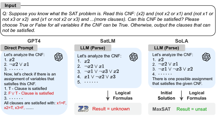
Figure 1: Exemplar specifications for arithmetic reasoning problems generated by different approaches. Direct prompt by GPT-4 makes errors when generating the variable assignment; SATLM based on the Z3 solver cannot solve this CNF and outputs unknown (both errors are highlighted in red). In contrast, SoLA is able to generate the correct answer by using the LLMs to parse CNF and generate an initial solution and relying on a MaxSAT layer to handle the reasoning.

3 Motivation

In this paper, our primary motivation is to explore the potential of enhancing the logical reasoning capability of Large Language Models (LLMs) by introducing a differential solver layer. Traditionally, the prevailing approaches either replace solvers with neural networks (Shi et al., 2022a) or directly utilize SAT solvers (Ye X, 2023). However, we posit the existence of a third approach, as the first two either isolate from the solver or overly rely on it. Our proposed method involves a fusion approach, seamlessly integrating the solver into the reasoning process of LLMs. In essence, we opt to ”differentialize the solver” to augment reasoning capabilities.

The second motivation for this research stems from an analysis of industrial SAT solving, marked by two distinctive features: (1) Its large scale, resulting in a rapid degradation of solver performance due to the exponential expansion of the search space; (2) The formidable challenge presented by the verification of arithmetic circuits, often requiring weeks or even months for resolution using current solvers. Both of these characteristics impose substantial limitations on the effectiveness of an LLM augmented with a solver in the domain of SAT solving.

Consequently, our objective is to identify a synergistic approach that combines the strengths of LLMs and solvers while sidestepping the limits of solvers. This approach aims to leverage the LLM’s capacity to comprehend logical formulas, while concurrently capitalizing on the solver’s refinement abilities to attain accurate solutions. Figure 1 illustrates an example that highlights the comparison between vanilla LLM, SatLM, and our proposed SoLA. The LLM alone may introduce logical flaws during inference, and SatLM may struggle with complex circuit problems due to its backbone solver’s limitations. In contrast, our proposed SoLA can produce accurate answers through the collaboration of LLM and the differential solver layer.

4 Theoretical Analysis

4.1 Preliminaries

In modern SAT solving, the input is typically a CNF formula denoted as $\phi(v_{1},\dots,v_{n})$, which is a conjunction of clauses $\omega$. Each clause represents a disjunction of literals, where a literal is either a variable $v_{i}$ or its complement $\neg v_{i}$. Variables can be assigned logic values, either $1$ or $-1$, representing True or False, respectively . An SAT solver is designed to determine either a satisfying assignment for a given formula $\phi$ or conclusively demonstrate its unsatisfiability (UNSAT). If the formula is unsatisfiable, the solver will produce an unsatisfiable core, which is a subset of clauses from the formula’s representation in conjunctive normal form that remains unsatisfiable. Contemporary SAT solvers are founded on the Conflict-Driven-Clause-Learning (CDCL) algorithm, with numerous data-driven methods integrated into CDCL to enhance computational efficiency.

In this study, we define a CNF dataset denoted as $\mathcal{D}$, consisting of input-output pairs $(x_{i},y_{i})$, where $x_{i}$ represents a logical formula and $y_{i}$ indicates its satisfiability status (either SAT or UNSAT). When a CNF formula is fed into an LLM, our goal is to determine its satisfiability and provide accurate assignments for satisfiable instances. To achieve this, we might incorporate a solver as an additional logic reasoner for the LLM. However, the exponential search complexity inherent in state-of-the-art SAT solvers poses a significant challenge, limiting their effectiveness on complex problems. Therefore, a key issue is how to design a solver layer that can both refine the LLM’s outputs effectively and efficiently address complex problems.

4.2 From SAT to Differential MaxSAT Formulations

Assuming that each CNF $\phi(v_{1},\dots,v_{n})$ comprises $n$ binary variables, with each $v_{i}\in\{1,-1\}$ ($i\in{1,2,\dots,n}$) representing a boolean variable. Each CNF is associated with a set of clauses (constraints), and each clause is defined on a subset of variables $S_{i}\subset V$, signifying the variables’ simultaneous legal assignments. In other words, when $S_{i}=\{v_{i_{1}},v_{i_{2}},\dots,v_{i_{r}}\}$, the constraints define a subset of the Cartesian product $\prod_{1}^{i_{r}}\{1,-1\}$. Let’s introduce the variable $\boldsymbol{s}_{i}\in\{-1,0,1\}^{m}$, where $s_{ij}$ denotes the sign of $v_{i}$ in clause $j\in{1,2,\dots,m}$. Consequently, we can establish a clause matrix $\boldsymbol{S}\in\{1,-1,0\}^{m\times n}$, where each element $s_{ij}$ in $\boldsymbol{S}$ signifies the sign of variable $\tilde{v}_{i}$ in clause $j$. Therefore, each SAT instance can be translated into a corresponding MaxSAT problem, wherein $\bigvee$ represents the logical “or” symbol,

$$\underset{\tilde{\boldsymbol{v}}\in\{-1,1\}^{n}}{\max}\sum_{j=1}^{m}\bigvee_{i=1}^{n}\textbf{1}\{s_{ij}\tilde{v}_{i}>0\}.$$ (1)

Furthermore, assuming that $\boldsymbol{v}=[\boldsymbol{v}_{d},\boldsymbol{v}_{1},\dots,\boldsymbol{v}_{n}]\in\mathbb{R}^{k\times(n+1)}$ and $\boldsymbol{S}=[\boldsymbol{s}_{d},\boldsymbol{s}_{1},\dots,\boldsymbol{s}_{n}]\in\mathbb{R}^{m\times(n+1)}$, by relaxing each discrete variable $\tilde{v}_{i}$ to a unit vector $\boldsymbol{v}_{i}\in\mathbb{R}^{k},\|\boldsymbol{v}_{i}\|=1$ with respect to a unit “truth direction” $\boldsymbol{v}_{d}$, we can further obtain the relaxation of MaxSAT in a semidefinite programming (SDP) problem based on Equation 1 as follows:

$$\underset{\boldsymbol{v}\in\mathbb{R}^{k\times(n+1)}}{\min}\langle\boldsymbol{S}^{\top}\boldsymbol{S},\boldsymbol{v}^{\top}\boldsymbol{v}\rangle,$$ (2)

$$\quad\text{s.t.}\;\|\boldsymbol{v}_{i}\|=1,i\in\{d,1,2,\dots,n\}.$$

Additionally, you can find that Equation 2 is low-rank and each coefficient vector $\boldsymbol{s}_{d}=\{-1\}^{m}$ is associated with the truth vector. Considering the conclusions that the low-rank SDP formulation has been shown to recover the optimal SDP solution given $k>\sqrt{2n}$ (Pataki, 1998), we set $k=\sqrt{2n}+1$ to recover the optimal solution of the original MaxSAT problem in Equation 1. Given the binary input variables $v_{i}$ in Equation 2, the solver layer first relaxes them to unit vectors and then solves Equation 2 optimally to obtain the output variable assignments by fast coordinate descent for all $o\in\mathcal{O}$. Hereby, each output vector $\boldsymbol{v}_{o}$ can be updated iteratively as $\boldsymbol{v}_{o}=-\boldsymbol{g}_{o}/\|\boldsymbol{g}_{o}\|$, where $\boldsymbol{g}_{o}=\boldsymbol{v}\boldsymbol{S}^{\top}\boldsymbol{s}_{o}-\|\boldsymbol{s}_{o}\|^{2}\boldsymbol{v}_{o}$. It is evident that the SDP problem represents a convex hull of the MaxSAT problem, and the optimal solutions of the MaxSAT problem can be approximated using the coordinate descent approach. Furthermore, due to the unit vector constraint in Equation 2, the time complexity for solving the SDP problem is polynomial (Wang et al., 2019), making it more computationally efficient than the original MaxSAT problem with exponential time complexity.

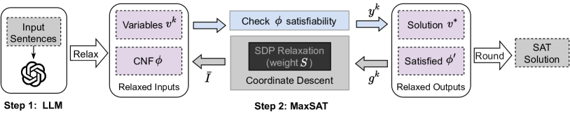
Figure 2: The flow of SoLA. Starting from a problem in natural language, in Step 1, the LLM parses logic formulas and outputs an initial solution. In Step 2, the relaxed variables and extracted CNF are offloaded to a MaxSAT solver layer, checking the satisfiability of clauses, and producing the solution to the SAT problem. Here, the blue arrows indicate the forward pass, while the grey arrows represent the backward pass.

4.3 Towards SAT Solving

Supposing that the approximate optimal solution of MaxSAT in Equation 1 is given as $\mathcal{C}(v_{1},v_{2},\dots,v_{n})$, and it is easy to check whether this assignment can satisfy the original SAT problem $\phi$. A trivial case is that if all the clauses (i.e., constraints) are satisfied by the assignments $\mathcal{C}(v_{1},v_{2},\dots,v_{n})$, then these assignments constitute a valid solution for the original SAT problem $\phi$. In the scenario where $\mathcal{C}(v_{1},v_{2},\dots,v_{n})$ satisfies only a subset of the clauses, we denote the clauses that cannot be satisfied as $\bar{\phi}$—a subset of all clauses—and identify the indices of the variables in $\bar{\phi}$ as $\bar{I}$. The MaxSAT problem aims to produce a satisfiable subset of clauses in $\phi$ with the maximum cardinality. This problem can be approximated as an SDP problem, represented as a convex hull, with its coordinate descent yielding minimal solutions within the sub-convex hull. It is evident that solving each satisfied problem involves constructing a series of SDP problems. In practice, due to the computational cost associated with updating all literals, we choose to update only the variables in the sub-convex hull, referred to as $\bar{I}$, to progressively approach the final solutions.

Assuming that the LLM is initially provided with a CNF and can derive the initial assignments for all literals, we can employ the solver to verify whether this set of assignments satisfies all constraints. In cases where the constraints are not satisfied, the LLM can be enhanced through an additional layer, namely the MaxSAT relaxation of the original CNF expression, to iteratively update the variable assignment until all clauses are satisfied. The details of the operation of the MaxSAT layer are presented in Section 5.2.

4.4 Towards UNSAT Proving

In general, an UNSAT instance denotes that, over all possible assignments of the literals, there exist at least two clauses that cannot be satisfied simultaneously. Let’s consider the CNF formula $\phi$, where $S$ is a subset of variables, and $D$ defines the solution space. In the theory of satisfiability, the following lemma is based on the backdoor counting results (Williams et al., 2003),

Lemma 1 Given a CNF formula $\phi$ with $n$ variables, for all subsets $S$ of the $n$ variables with $|S|=i$, perform a standard backtracking search (solely on the variables in $S$) for an assignment that resolves $C$. The search time for finding this assignment is $O\left(p(n)\frac{dn}{B(n)^{1/2}}^{B(n)}\right)$, where $p(n)$ is some polynomial.

Therefore, based on Lemma 1, we can have a conclusion for UNSAT proving:

Theorem 1 Considering the structure of the search tree, if every leaf in the search tree concludes with sub-assignments indicating unsatisfiability, the original CNF formula $\phi$ is deemed UNSAT with a probability of 1.

The proof is evident. Each leaf of the search tree represents a partial assignment for the original formula $\phi$. It is clear that if all partial assignments indicate the existence of two clauses that cannot be satisfied simultaneously, the formula is UNSAT. Returning to the LLM for SAT solving, when the LLM is given a CNF, it can at least provide an assignment that satisfies part of the original clauses. Based on Lemma 1 and Theorem 1, the problem can be refined to the final solution in polynomial time. If, in some iterations, all subproblems are found to be UNSAT, then the original problem is UNSAT. We can further draw the following conclusions, culminating in the complete proof of UNSAT scenarios:

Corollary 1 If all leaves end with the sub-assignments reporting satisfiability, we can always get a minimal unsatisfied assignment by adding constraints in polynomial loops.

Now the problem of UNSAT proving involves efficiently finding the unsatisfied subproblem. Here we we illustrate our approach with a simple example. Clearly, $\phi=(x_{1})\wedge(\neg x_{1})\wedge(\neg x_{1}\vee x_{2})\wedge(\neg x_{2})$ has a MaxSAT solution with three satisfied clauses: $(\neg x_{1})\wedge(\neg x_{1}\vee x_{2})\wedge(\neg x_{2})$. Consider $(x_{1})$, the clause not included in the MaxSAT solution, it provides useful information. If it is removed from $\phi$, the resulting formula is satisfiable. Therefore, we denote such clauses as $\bar{\phi^{\prime}}$, where $\phi^{\prime}$ is the MaxSAT solution of $\phi$. In other words, $\bar{\phi^{\prime}}$ is a complementary set of $\phi^{\prime}$.

This complementary view of $\phi^{\prime}$ reveals another connection between maximum satisfiability and minimally unsatisfiable cores (MUC). Particularly, a minimally unsatisfiable core is an unsatisfiable subset of the clauses in such that removing any clause from the set makes it satisfiable. In other words, none of the clauses in the core are superfluous, i.e., deleting any singleton clause from MUC will cause it to be satisfiable. Because the presence of any MUC in a formula makes it unsatisfiable, at least one clause from every MUC must be removed to make it satisfiable. That is, given an unsatisfiable formula $\phi$ and a set of clauses $\gamma\subseteq\phi$, $\phi^{\prime}=\phi\backslash\gamma$ is satisfiable if and only $\gamma$ contains at least one clause from $\bar{\phi^{\prime}}$. Therefore, $\bar{\phi^{\prime}}$ must contain at least one clause from minimally unsatisfiable subformulas. As the maximum satisfiable set $\phi^{\prime}$ can be readily obtained by its SDP relaxation, i.e., Equation 2, surely we can leverage its complement $\bar{\phi^{\prime}}$ to iteratively find unsatisfiable subproblems (see more details in Section 5.3).

5 Algorithm

5.1 Overview

In this section, we present SoLA, which augments LLM with the ability of logical reasoning by incorporating a differential MaxSAT layer. More specifically, SoLA addresses the challenge of using LLMs to tackle logical reasoning tasks expressed in natural language. These tasks typically involve presenting a set of premises and constraints, prompting questions that necessitate intricate deductive reasoning over the provided inputs, which remains a formidable challenge even for contemporary LLMs (Valmeekam et al., 2022).

At a high level, given the natural language description of a collection of facts $\phi$ (such as propositions or constraints) about some variables $V$, the LLM is asked to determine the satisfiability of $\phi$ and find assignments of these variables if $\phi$ can be satisfied. To address this, SoLA first applies an LLM to parse the logic formula and, if possible, generate an initial solution. Then, a differential MaxSAT layer, functioning as a solver, is employed to refine this initial solution. Fig. 2 provides an overview of the proposed SoLA approach.

Indeed, the MaxSAT layer, seamlessly integrated into the framework, operates without any trainable parameters and necessitates no training datasets or labels. Its operations are solely dictated by a set of logical formulas $\phi$. In contrast to SATNet (Wang et al., 2019), which embeds problem-specific CNF structures in its weights through data-driven training, our proposed MaxSAT layer does not require training and exhibits greater generality when addressing diverse problems. In comparison to SMTLayer (Wang et al., 2023), which relies on an off-the-shelf solver for reasoning, the MaxSAT layer bypasses the constraints imposed by current solvers and eliminates the need for labels.

5.2 MaxSAT Layer

In Section 4.2, we approximate the original satisfiability (SAT) problem as a Maximum Satisfiability (MaxSAT) problem, in which the goal is to find an assignment that maximizes the number of satisfied clauses. Furthermore, we can achieve fast solving for the MaxSAT problem via SDP relaxation and associated coordinate descent. Using the differentiation of the SAT problem, we create a MaxSAT layer at the top of LLM for SAT solving. We now present the details of the forward and backward passes of our proposed MaxSAT layer.

Forward Pass. The forward pass algorithm is outlined in Algorithm 1. In the forward pass, the inputs consist of relaxed solutions and CNFs parsed by the language model. Subsequently, the layer transforms these inputs by extracting the sign of the variables, thereby casting them to Boolean values. The layer then assesses the satisfiability of $\phi^{\prime}$ (line2). If the current variable assignment satisfies $\phi^{\prime}$, the MaxSAT layer outputs $y^{k}$ as True, indicating that $\phi$ is satisfied and a feasible solution for the given CNF has been identified. Conversely, if $\phi$ cannot be satisfied, the MaxSAT layer outputs $y^{k}$ as False, prompting the initiation of the backward pass to update the variable assignment.

Algorithm 1 The forward pass of MaxSAT layer

0:  Variable assignment $\boldsymbol{v}^{k}\in\mathbb{R}^{p}$ at $k$-th epoch, conjunctive constraints formula $\phi$.

0:  $y^{k}$, solution $\boldsymbol{v}^{*}$.

1:  $\tilde{v}^{k}\leftarrow[\boldsymbol{v}^{k}_{i}>0:i=1,\dots,p]$;

2:  $\phi^{\prime}\leftarrow\phi(\tilde{v}^{k}_{1},\dots,\tilde{v}^{k}_{p})$;

3:  if $\phi^{\prime}$ is satisfiable then

4:     $y^{k}\leftarrow$ True;

5:     $\boldsymbol{v}^{*}\leftarrow\boldsymbol{v}^{k}$ ;

6:  else

7:     $y^{k}\leftarrow$ False;

8:  end if

Backward Pass. Algorithm 2 illustrates our backward pass. The backward pass is responsible for computing the gradient of the layer inputs and derive updates to variables that steer toward satisfying constraints $\phi$. The key issue of the backward pass involves identifying which input variables might have contributed to the unsatisfiability of constraint formulas. Drawing from the theoretical analysis presented in Section 4.3, it is established that variables in $\bar{\phi^{\prime}}$ constitute the unsatisfiable core and are, therefore, more likely to be sources of conflict. Variables not present in $\bar{I}$ have their gradients set to zero, as their absence in the core does not provide evidence regarding the correctness or incorrectness of these inputs.

After obtaining the maximal set of variables that are consistent with logic formulas $\phi^{\prime}$ (line 5), we proceed to compute the gradient at each variable not belonging to this set. More specifically, this gradient computation employs the Binary Cross-Entropy (BCE) loss for $v_{i}$ concerning its counterfactual counterpart, $1-\text{sign}(v_{i})$ (line 7). In this way, we update variables in a direction that would have modified the inputs such that they are not in the unsatisfiable core. Subsequently, employing a predefined learning rate $\lambda$, we engage in gradient descent towards $\boldsymbol{v}^{k}$ (line 10). This iterative process yields variable assignments that have the potential to satisfy more constraint formulas within $\phi$.

Algorithm 2 The backward pass of MaxSAT layer

0:  $\boldsymbol{v}^{k}\in\mathbb{R}^{p}$ from forward pass, $y^{k}$ from forward pass, CNF $\phi$, learning rate $\lambda$.

0:  Gradient $\boldsymbol{g}^{k}$ of $\boldsymbol{v}^{k}$, updated assignment $\boldsymbol{v}^{k+1}$.

1:  $\boldsymbol{g}^{k}\leftarrow\emph{0}$;

2:  if $y^{k}$ is False then

3:     $\tilde{v}^{k}\leftarrow[\boldsymbol{v}^{k}_{i}>0:i=1,\dots,p]$;

4:     $\phi^{\prime}\leftarrow\phi(\tilde{v}^{k}_{1},\dots,\tilde{v}^{k}_{p})$;

5:     $I\leftarrow\arg\max_{I\subseteq[1,p]}\phi^{\prime}\wedge\bigwedge_{i\in[1,p]}v_{i}=\tilde{v}^{k}_{i}$;

6:     for $i\in\bar{I}$ do

7:        $g^{k}_{i}\leftarrow\partial_{\boldsymbol{v}^{k}_{i}}\mathcal{L}(\boldsymbol{v}^{k}_{i},1-\text{sign}(\boldsymbol{v}^{k}_{i}))$;

8:     end for

9:  end if

10:  Update $\boldsymbol{v}^{k+1}\leftarrow\boldsymbol{v}^{k}-\lambda\boldsymbol{g}^{k}$;

5.3 From MaxSAT to SAT Solving and UNSAT Proving

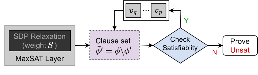
Figure 3: This figure illustrates our approach to proving a problem as UNSAT. We iteratively examine the satisfiability of $\hat{\phi^{\prime}}$ , extract the corresponding literals, and expand the clause set based on the relevant literals to identify an unsatisfiable subformula.

In this section, we outline the process of solving an SAT problem using the MaxSAT layer, with the stopping criterion being the stability of the MaxSAT solution. Compared to the UNSAT problem, solving the SAT problem is relatively straightforward since the solution to the MaxSAT problem directly corresponds to the solution of the original SAT problem with all clauses satisfied. Therefore, upon achieving a satisfiable variable assignment through multiple forward and backward passes, it can be inferred that the constraint formula is SAT, and the solution can be directly output. On the other hand, addressing the UNSAT problem involves additional steps. Specifically, the key to tackling the UNSAT problem is identifying the unsatisfied subproblem. As per the theoretical analysis in Section 4.4, the complementary set of $\phi^{\prime}$ must include at least one clause from minimally unsatisfiable subformulas.

Fig.3 illustrates our UNSAT-proving process. We commence by checking the satisfiability of $\hat{\phi^{\prime}}$ using a SAT solver. If this subset is UNSAT, we have successfully identified the unsatisfiable subproblem and completed the UNSAT-proving process. If it is satisfied, indicating that the unsatisfiable core is not included, we extract all variables from this subset and introduce new clauses involving these variables to create a new clause set. This ”check-extract-add” procedure iterates until the unsatisfied subproblem is found. Using the instances in Figure 3 as an example, as $(x_{1})$ is the clause not included in the MaxSAT solution, we first check the satisfiability of ${(x_{1})}$, which is SAT. Next, we extract the variable $x_{1}$ along with the corresponding clauses $(\neg x_{1})$ and $(\neg x_{1}\vee x_{2})$, both containing $x_{1}$. By checking the new clause set, i.e., $(x_{1})\wedge(\neg x_{1})\wedge(\neg x_{1}\vee x_{2})$, it becomes evident that it is UNSAT due to the conflicting $(x_{1})\wedge(\neg x_{1})$. Considering Corollary 14.4, we can consistently obtain such an unsatisfied core in polynomial loops, a significantly more efficient approach compared to the CDCL-based SAT solver with exponential complexity.

6 Experiments

In this section, we present an empirical evaluation of SoLA on solving SAT problems expressed by natural language. Particularly, we test our approach in both SAT and UNSAT datasets. For satisfiable instances, LLMs need to determine the CNF instance’s satisfiability and output the variable assignments that genuinely satisfy the input CNF instance, while in the case of UNSAT instances, deep models are tasked with efficiently proving the unsatisfiability of CNFs.

Our results demonstrate the following primary findings. 1) SoLA can significantly improve the inference accuracy of LLM, achieving a perfect accuracy rate of 100% for both SAT and UNSAT datasets with as many as 200 variables. 2) When dealing with large circuit cases, SoLA outperforms state-of-the-art solvers, including Z3 (De Moura & Bjørner, 2008) and kissat (Biere & Fleury, 2022), showcasing exceptional efficiency in solving complex problems.

Table 1: Accuracy and runtime (s) of GPT-4, SATLM, and our method (SoLA, LLM with solver layer adaptation) on both SAT and UNSAT datasets.

Problem	Number of Literals	GPT-4		SATLM		SoLA
		Accuracy(%)	Time(s)	Accuracy(%)	Time(s)	Accuracy(%)	Time(s)
SAT	3	46	12.80	100	12.81	100	12.81
	10	12	20.42	100	20.43	100	20.43
	20	-	-	100	0.01	100	0.03
	50	-	-	100	0.02	100	0.06
	100	-	-	100	0.06	100	0.16
	200	-	-	100	3.11	100	4.39
UNSAT	3	21	12.56	100	12.57	100	12.66
	10	0	19.28	100	19.29	100	19.38
	20	-	-	100	0.02	100	1.59
	50	-	-	100	0.05	100	2.27
	100	-	-	100	0.21	100	4.28
	200	-	-	100	117.51	100	6.05

6.1 Experimental Setting

Datasets: We conducted experiments on both open-source satisfiability problems  and intricate industrial cases, challenging for state-of-the-art SAT solvers that may require several weeks to handle. Specifically, we opted to assess our approach on open-source datasets featuring 3, 10, 20, 50, 100, and 200 variables, each containing 50 satisfiable and 50 unsatisfiable instances. As our datasets are encoded in conjunctive normal form, such as $(x1\vee x2)\wedge(\neg x2\vee x3)$, we transform these constraints into text by substituting $\vee$ with or, $\wedge$ with and, and $\neg$ with not. Consequently, the constraints are articulated in natural language, for instance, (x1 or x2) and (not x2 or x3), enabling them to be input into LLMs with prompts. For challenging industrial cases, we selected the formal verification problem of high bit-width multipliers and hybrid multiply-add circuits. These instances frequently pose difficulties for modern SAT solvers, often causing them to enter into an infinite loop and thus taking several weeks to solve.

We conducted a comparative analysis between SoLA and two baseline methods, namely SATLM (Ye X, 2023) and GPT-4 (Achiam et al., 2023). In particular, SATLM (Ye X, 2023) employs an LLM to parse problem specifications and offloads the logical reasoning task to the Z3 solver (De Moura & Bjørner, 2008). We implement a prototype of our proposed SoLA using Pytorch (Paszke et al., 2019), with GPT-4 as a backbone model to parse CNF and generate an initial solution. It’s noteworthy that the MaxSAT layer within SoLA requires no training labels and is adaptable to problem types expressed in Boolean variables. We configured the learning rate of the MaxSAT layer to be 1, facilitating the effective flipping of selected variables. Additionally, the maximum number of epochs was set to 50.

6.2 SAT and UNSAT Problem

We report the accuracy and time of SoLA and baselines in Table 1. The reported time encompasses both the LLM inference time and solving time. It’s important to note that for CNFs with more than 20 variables, the standalone LLM struggles to handle such complexity. In such cases, the large language model functions as a parser, and we compare the accuracy and solving time of the Z3 solver against our proposed MaxSAT layer. Analysis of Table 1 reveals that both solver-based SATLM and SoLA achieve 100% accuracy when handling problems with 3, 10, 20, 50, 100, and 200 literals. For all SAT instances and UNSAT instances with fewer than 200 literals, SATLM exhibits faster performance than SoLA. However, in the case of the UNSAT problem with 200 literals, the runtime of SATLM is 19 $\times$ greater than that of SoLA due to the exponential complexity of the Z3 solver. This experiment on smaller cases underscores the accuracy of the differential MaxSAT layer in SAT solving.

6.3 Solver-Incapable Industrial Problem

Compared with SATLM (Ye X, 2023), which relies on an off-the-shelf solver to perform reasoning, SoLA sidesteps the limitations of the SAT solver itself, such as high computational cost when dealing with complex formulas. In practice, there exist intricate industrial cases where even the SOTA SAT solvers struggle and may take weeks to solve. These challenging industrial instances often involve unsatisfiable arithmetic circuits. Here we leverage the state-of-the-art SMT solver, i.e., z3 (De Moura & Bjørner, 2008), and SAT solver, i.e., kissat (Biere & Fleury, 2022), as our baselines. The experimental results in Table 2 reveal that SoLA outperforms SOTA SAT solvers significantly in solving hard cases. Notably, it can solve cases 4, 5, and 6 within 1 minute, while the two other solvers cannot tackle them within 24 hours. The results on hard cases demonstrate the high efficiency of our differential MaxSAT layer.

Table 2: Runtime (s) of z3, kissat, and our MaxSAT layer on solving hard industrial dataset.

Test case	# Clauses	Z3	Kissat	SoLA
case1	1122	>24h	160.32	11.61
case2	1122	>24h	171.13	11.80
case3	1610	>24h	10556.56	16.03
case4	2190	>24h	>24h	20.83
case5	3909	>24h	>24h	36.32
case6	6169	>24h	>24h	57.91

7 Conclusion

Addressing the challenges posed by the limitations of Large Language Models (LLMs) in logical reasoning and symbolic solvers in handling industrial hard cases, this paper introduces a pioneering method named Solver-layer Adaption (SoLA). In SoLA, a solver is integrated as a layer within the LLM. By establishing appropriate forward and backward pass gradients, the solver layer collaborates with the LLM, refining its outputs and guiding the convergence to final solutions within a polynomial loop, or proving unsatisfiability. Extensive experiments demonstrate the effectiveness of SoLA in enhancing the logical reasoning ability of LLMs for both SAT and UNSAT instances, outperforming state-of-the-art GPT-4 while maintaining comparable runtime to symbolic solvers and existing tool-learning methods. Notably, for challenging industrial instances, SoLA accurately estimates UNSAT cores, showcasing convergence to an accurate UNSAT core within polynomial loops. The results suggest that SoLA achieves new state-of-the-art performance in symbolic logical reasoning tasks, paving the way for harnessing solver capabilities to enhance the logical learning capabilities of LLMs.

Appendix A Appendix

In this section, we illustrate the detailed solving process for two cases: an easy SAT problem that yields results within 2 epochs, and a complex UNSAT problem that only provides the solution to its MaxSAT relaxation. We start with the easy SAT problem, which entails 50 variables. Initially, all variables are set to False, and this initial assignment fails to satisfy the CNF, necessitating changes to some variable values during the backward pass. Specifically,

• In the forward pass, we evaluate whether the current variable assignment satisfies all clauses. If it does not, the output $y$ is set to 0, indicating the need to enter the refinement loop to obtain the final solutions.

• In the backward pass, following the resolution of the MaxSAT problem, we isolate the constraints not included in the satisfied clause set and extract the indices of variables associated with these unsatisfied constraints. Using $\bar{I}$, we update the values of unsatisfied variables via gradient descent to ensure they are not part of the unsatisfiable core.

The detailed solving process for this easy problem is listed as follows:

Table 3: The details of the solving process of the easy problem, where green numbers indicate the sign of updated variables.

# Epoch	Unsatisfied Variable Indice	Variable Assignment	y
0	9, 10, 13, 14, 17, 18, 19, 24, 27, 28, 29, 30, 31, 32, 34, 37, 40, 41, 45, 48, 49	-1, -1, -1, -1, -1, -1, -1, -1,-1, 1, 1, -1, -1, 1, 1, -1, -1, 1, 1, 1, -1, -1, -1, -1, 1, -1, -1, 1, 1, 1, 1, 1, 1, -1, 1, -1, -1, 1, -1, -1,-1, 1, -1, -1, -1, 1, -1, -1, 1, 1	0
1	43	-1, -1, -1, -1, -1, -1, -1, -1,-1, 1, 1, -1, -1, 1, 1, -1, -1, 1, 1, 1, -1, -1, -1, -1, 1, -1, -1, 1, 1, 1, 1, 1, 1, -1, 1, -1, -1, 1, -1, -1,-1, 1, -1, 1, -1, 1, -1, -1, 1, 1	1

For comparison, we add the response of GPT-4 for the same problem in Fig. 4, from which we can see that GPT-4 cannot analyze such an SAT problem with 50 variables.

Figure 4: Response illustration of GPT-4.

For the complex UNSAT problem, we focus on elucidating the process of deriving the unsatisfiable subproblem based on the complement of the MaxSAT solution, as the steps for solving the MaxSAT relaxation mirror those of the SAT problem. Specifically, this problem encompasses 2,620 variables and 10,732 clauses, and the solver to check the satisfiability of the subproblem is Kissat. Throughout the forward and backward passes of the MaxSAT layer, we iteratively adjust the variable assignments to maximize the number of satisfied clauses. However, given the nature of this problem being UNSAT, our objective is not to obtain a solution with all clauses satisfied, but rather to achieve a variable assignment that satisfies as many clauses as possible. Specifically, in the context of such UNSAT problems, we halt the MaxSAT layer when the number of satisfied clauses reaches a plateau and remains unchanged.

We list the detailed attempt to generate an unsatisfied subproblem in Table 4. After solving the MaxSAT problem of our complex UNSAT case, the only clause left in the unsatisfied clause set is $\{\neg v2\}$, so we begin with this clause set. Clearly, this CNF with only 1 clause is satisfiable, so we extract the variable in it, i.e., $v2$. Then, we begin our iteration 2, i.e., select more clauses with $v2$ and add these new clauses to the clause set. Specifically, in iteration 2, we add 4 new clauses with $v2$, ending up with 5 clauses with 3 variables. After checking with the Kissat solver, this clause set is still SAT, so we extract all variables from it and add more related clauses. This ”check-extract-add” procedure iterates until we have 10731 clauses with 2618 variables in the 14th iteration, and the solver cannot determine the solution of this subproblem in 24 hours. Indeed, we can say that this complex CNF is largely UNSAT as its MaxSAT solution is smaller than the number of clauses. However, due to its complex structure, we cannot find the unsatisfiable subproblem through the SOTA solver.

We outline the detailed process of attempting to generate an unsatisfied subproblem in Table 4. In our complex UNSAT case, following the resolution of the MaxSAT problem, only the clause ${\neg v2}$ remains in the unsatisfied clause set. Thus, we initiate the process with this solitary clause. However, this CNF, comprising only one clause, is evidently satisfiable. Subsequently, we proceed to iteration 2, wherein we select additional clauses containing $v2$ and incorporate them into the clause set. Specifically, in iteration 2, we introduce four new clauses involving $v2$, resulting in a set of five clauses comprising three variables. The resulting clause set remains satisfiable upon evaluation by the Kissat solver. This ”check-extract-add” procedure iterates until the 14th iteration, where the clause set comprises 10,731 clauses with 2,618 variables. However, the solver fails to ascertain the solution to this subproblem within 24 hours. Notably, while the MaxSAT solution indicates the unsatisfiability of the complex CNF, with the number of clauses exceeding the solution size, the intricate structure of this complex CNF renders identification of the unsatisfiable subproblem challenging for state-of-the-art solvers. Therefore, given the limitations posed by SOTA solvers, there are instances where identifying the unsatisfiable subproblem proves challenging. Despite this limitation, we can still offer the solution to the MaxSAT relaxation of such problems. While this solution may not directly address the unsatisfiable core, it can serve as a valuable resource for subsequent resolution attempts.

Table 4: The details of finding an unsatisfied subproblem for a complex problem.

Iteration	# Variables in subproblem	# Clauses in subproblem	Solver time (s)	Solver result
0	1	1	<0.00001	SAT
1	3	5	0.004	SAT
2	7	13	0.004	SAT
3	17	33	0.006	SAT
4	41	80	0.01	SAT
5	98	203	0.02	SAT
6	222	499	0.05	SAT
7	396	1096	0.11	SAT
8	646	1796	0.23	SAT
9	1006	2936	0.46	SAT
10	1677	4941	1.05	SAT
11	2321	8511	2.69	SAT
12	2583	10326	4.26	SAT
13	2618	10706	5.38	SAT
14	2618	10731	>24h	Unknow

References

- Achiam et al. (2023) Achiam, J., Adler, S., Agarwal, S., Ahmad, L., Akkaya, I., Aleman, F. L., Almeida, D., Altenschmidt, J., Altman, S., Anadkat, S., et al. Gpt-4 technical report. arXiv preprint arXiv:2303.08774, 2023.
- Becker et al. (2014) Becker, B., Drechsler, R., and Sauer, M. Recent advances in sat-based atpg: Non-standard fault models, multi constraints and optimization. Proc. DTTIS, pp. 1–10, 2014.
- Biere & Fleury (2022) Biere, A. and Fleury, M. Gimsatul, IsaSAT and Kissat entering the SAT Competition 2022. In Balyo, T., Heule, M., Iser, M., Järvisalo, M., and Suda, M. (eds.), Proc. of SAT Competition 2022 – Solver and Benchmark Descriptions, volume B-2022-1 of Department of Computer Science Series of Publications B, pp. 10–11. University of Helsinki, 2022.
- De Moura & Bjørner (2008) De Moura, L. and Bjørner, N. Z3: An efficient smt solver. In International conference on Tools and Algorithms for the Construction and Analysis of Systems, pp. 337–340. Springer, 2008.
- Feng et al. (2023a) Feng, J., Xu, R., Hao, J., Sharma, H., Shen, Y., Zhao, D., and Chen, W. Language models can be logical solvers. arXiv preprint arXiv:2311.06158, 2023a.
- Feng et al. (2023b) Feng, X., Wan, Z., Wen, M., Wen, Y., Zhang, W., and Wang, J. Alphazero-like tree-search can guide large language model decoding and training. arXiv preprint arXiv:2309.17179, 2023b.
- Kurin et al. (2020) Kurin, V., Godil, S., Whiteson, S., and Catanzaro, B. Can q-learning with graph networks learn a generalizable branching heuristic for a sat solver? Advances in Neural Information Processing Systems, 33:9608–9621, 2020.
- Langley (2000) Langley, P. Crafting papers on machine learning. In Langley, P. (ed.), Proceedings of the 17th International Conference on Machine Learning (ICML 2000), pp. 1207–1216, Stanford, CA, 2000. Morgan Kaufmann.
- Li et al. (2022) Li, M., Shi, Z., Lai, Q., Khan, S., Cai, S., and Xu, Q. Deepsat: An eda-driven learning framework for sat. arXiv preprint arXiv:2205.13745, 2022.
- Lightman (2023) Lightman, Hunter, e. a. Let’s verify step by step. arXiv:2305.20050., 2023.
- Nguyen et al. (2023) Nguyen, H.-T., Fungwacharakorn, W., and Satoh, K. Enhancing logical reasoning in large language models to facilitate legal applications. arXiv preprint arXiv:2311.13095, 2023.
- Pan et al. (2023) Pan, L., Albalak, A., Wang, X., and Wang, W. Y. Logic-lm: Empowering large language models with symbolic solvers for faithful logical reasoning. arXiv preprint arXiv:2305.12295, 2023.
- Paszke et al. (2019) Paszke, A., Gross, S., Massa, F., Lerer, A., Bradbury, J., Chanan, G., Killeen, T., Lin, Z., Gimelshein, N., Antiga, L., et al. Pytorch: An imperative style, high-performance deep learning library. Advances in neural information processing systems, 32, 2019.
- Pataki (1998) Pataki, G. On the rank of extreme matrices in semidefinite programs and the multiplicity of optimal eigenvalues. Mathematics of operations research, 23(2):339–358, 1998.
- Selsam et al. (2018) Selsam, D., Lamm, M., Bünz, B., Liang, P., de Moura, L., and Dill, D. L. Learning a sat solver from single-bit supervision. arXiv preprint arXiv:1802.03685, 2018.
- Shi et al. (2022a) Shi, Z., Li, M., Khan, S., Zhen, H.-L., Yuan, M., and Xu, Q. Satformer: Transformer-based unsat core learning. In 2023 IEEE/ACM International Conference on Computer Aided Design (ICCAD), 2022a.
- Shi et al. (2022b) Shi, Z., Pan, H., Li, M., Khan, S., Zhen, H.-L., Yuan, M., and Xu, Q. Deepgate2: Functionality-aware circuit representation learning. arXiv:2305.16373., 2022b.
- Valmeekam et al. (2022) Valmeekam, K., Olmo, A., Sreedharan, S., and Kambhampati, S. Large language models still can’t plan (a benchmark for llms on planning and reasoning about change). arXiv preprint arXiv:2206.10498, 2022.
- Vlastelica et al. (2019) Vlastelica, M., Paulus, A., Musil, V., Martius, G., and Rolínek, M. Differentiation of blackbox combinatorial solvers. arXiv preprint arXiv:1912.02175, 2019.
- Wang et al. (2019) Wang, P.-W., Donti, P., Wilder, B., and Kolter, Z. Satnet: Bridging deep learning and logical reasoning using a differentiable satisfiability solver. In International Conference on Machine Learning, pp. 6545–6554. PMLR, 2019.
- Wang et al. (2023) Wang, Z., Vijayakumar, S., Lu, K., Ganesh, V., Jha, S., and Fredrikson, M. Grounding neural inference with satisfiability modulo theories. Thirty-seventh Conference on Neural Information Processing Systems, 2023.
- Williams et al. (2003) Williams, R., Gomes, C. P., and Selman, B. Backdoors to typical case complexity. IJCAI, 3:1173–1178, 2003.
- Xiong et al. (2024) Xiong, S., Payani, A., Kompella, R., and Fekri, F. Large language models can learn temporal reasoning. arXiv preprint arXiv:2401.06853, 2024.
- Ye X (2023) Ye X, Chen Q, D. I. Satlm: Satisfiability-aided language models using declarative prompting. Thirty-seventh Conference on Neural Information Processing Systems., 2023.
- Zhang et al. (2020) Zhang, W., Sun, Z., Zhu, Q., Li, G., Cai, S., Xiong, Y., and Zhang, L. Nlocalsat: Boosting local search with solution prediction. arXiv preprint arXiv:2001.09398, 2020.
- Zhang et al. (2023) Zhang, Y., Zhen, H.-L., Yuan, M., and Yu, B. Differential boolean difference for equivalence checking. Submitted to DAC, 2023.