Abstract

It is well-known that the reparameterisation gradient estimator, which exhibits low variance in practice, is biased for non-differentiable models. This may compromise correctness of gradient-based optimisation methods such as stochastic gradient descent (SGD). We introduce a simple syntactic framework to define non-differentiable functions piecewisely and present a systematic approach to obtain smoothings for which the reparameterisation gradient estimator is unbiased. Our main contribution is a novel variant of SGD, Diagonalisation Stochastic Gradient Descent, which progressively enhances the accuracy of the smoothed approximation during optimisation, and we prove convergence to stationary points of the unsmoothed (original) objective. Our empirical evaluation reveals benefits over the state of the art: our approach is simple, fast, stable and attains orders of magnitude reduction in work-normalised variance.

1 INTRODUCTION

In this paper we investigate stochastic optimisation problems of the form

$$\text{argmin}_{\boldsymbol{\theta}}\,\mathbb{E}_{\mathbf{z}\sim\mathbf{\mathcal{D}}_{\boldsymbol{\theta}}}[f_{\boldsymbol{\theta}}(\mathbf{z})]$$ (1)

which have a wide array of applications, ranging from variational inference and reinforcement learning to queuing theory and portfolio design (Mohamed et al.,, 2020; Blei et al.,, 2017; Zhang et al.,, 2019; Sutton and Barto,, 2018).

We are interested in scenarios in which $f_{\boldsymbol{\theta}}$ is directly expressed in a programming language. Owing to the presence of if-statements, which arise naturally when modelling real-world problems (see Section 6), $f_{\boldsymbol{\theta}}$ may not be continuous, let alone differentiable.

In variational inference, Bayesian inference is framed as an optimisation problem and $f_{\boldsymbol{\theta}}$ is the evidence lower bound (ELBO) $\log p(\mathbf{x},\mathbf{z})-\log q_{\boldsymbol{\theta}}(\mathbf{z})$, where $p$ is the model and $q_{\boldsymbol{\theta}}$ is a variational approximation. Our prime motivation is the advancement of variational inference for probabilistic programming—a new programming paradigm to pose and automatically solve Bayesian inference problems.

Gradient Based Optimisation.

In practice the standard method to solve optimisation problems of the form (1) are variants of Stochastic Gradient Descent (SGD). Since the objective function is in general not convex, we cannot hope to always find global optima and we seek stationary points instead, where the gradient w.r.t. the parameters ${\boldsymbol{\theta}}$ vanishes (Robbins and Monro,, 1951).

A crucial ingredient for fast convergence to a correct stationary point is an estimator of gradients of the objective function $\mathbb{E}_{\mathbf{z}\sim\mathbf{\mathcal{D}}_{\boldsymbol{\theta}}}[f_{\boldsymbol{\theta}}(\mathbf{z})]$ which is both unbiased and has low variance.

The Score or REINFORCE estimator (Ranganath et al.,, 2014; Wingate and Weber,, 2013; Minh and Gregor,, 2014) makes little assumptions about $f_{\boldsymbol{\theta}}$ but it frequently suffers from high variance resulting in suboptimal results or slow/unstable convergence.

An alternative approach is the reparameterisation or pathwise gradient estimator. The idea is to reparameterise the latent variables $\mathbf{z}$ in terms of a known base distribution (entropy source) via a diffeomorphic transformation ${\boldsymbol{\phi}}_{\boldsymbol{\theta}}$ (such as a location-scale transformation or cumulative distribution function). E.g. if $\mathbf{\mathcal{D}}_{\boldsymbol{\theta}}(z)$ is a Gaussian $\mathcal{N}(z\mid\mu,\sigma^{2})$ with ${\boldsymbol{\theta}}=\{\mu,\sigma^{2}\}$ then the location-scale transformation using the standard normal as the base gives rise to the reparameterisation

$$z\sim\mathcal{N}(z\mid\mu,\sigma^{2})\iff z=\mu+\sigma\,{s},\quad s\sim\mathcal{N}(0,1)$$

In general, $\mathbb{E}_{\mathbf{z}\sim\mathbf{\mathcal{D}}_{\boldsymbol{\theta}}}[f_{\boldsymbol{\theta}}(\mathbf{z})]=\mathbb{E}_{\mathbf{s}\sim\mathbf{\mathcal{D}}}[f_{\boldsymbol{\theta}}({\boldsymbol{\phi}}_{\boldsymbol{\theta}}(\mathbf{s}))]$ and its gradient can be estimated by (Mohamed et al.,, 2020):

$$\nabla_{\boldsymbol{\theta}}\,f_{\boldsymbol{\theta}}({\boldsymbol{\phi}}_{\boldsymbol{\theta}}(\mathbf{s}))\qquad\mathbf{s}\sim\mathbf{\mathcal{D}}$$

It is folklore that the reparameterisation estimator typically exhibits significantly lower variance in practice than the score estimator (e.g. Mohamed et al., (2020); Rezende et al., (2014); Fu, (2006); Schulman et al., (2015); Xu et al., (2019); Lee et al., (2018)). The reasons for this phenomenon are still poorly understood and examples do exist where score has lower variance than the reparameterisation estimator (Mohamed et al.,, 2020).

Unfortunately, the reparameterisation gradient estimator is biased for non-differentiable models, which can be easily expressed in a programming language by if-statements:

Example 1.1.

We recall a simple counterexample (Lee et al.,, 2018, Prop. 2).

$$\phi_{\theta}(s) \coloneqq s+\theta f(z) =-0.5\cdot z^{2}+\begin{cases}0&\text{if }z<0\\ 1&\text{otherwise}\end{cases}$$

Observe that (see Fig. 1(a)):

$$\nabla_{\theta}\,\mathbb{E}_{s\sim\mathcal{N}(0,1)}\left[f(\phi_{\theta}(z))\right] =-\theta+\mathcal{N}(-\theta\mid 0,1)$$

$$\neq-\theta=\mathbb{E}_{s\sim\mathcal{N}(0,1)}\left[\nabla_{\theta}f(\phi_{\theta}(s))\right]$$

Employing a biased gradient estimator may compromise the correctness of stochastic optimisation: even if we can find a point where the gradient estimator vanishes, it may not be a critical point of the objective function (1). Consequently, in practice we may obtain noticeably inferior results (see our experiments later, Fig. 2).

(a) Solid red: biased estimator $\mathbb{E}_{z\sim\mathcal{N}(0,1)}\left[\nabla_{\theta}f(\theta,z)\right]$, solid green: true gradient $\nabla_{\theta}\,\mathbb{E}_{z\sim\mathcal{N}(0,1)}\left[f(\theta,z)\right]$, black: gradient of smoothed objective (dotted: $\eta=1$, dashed: $\eta=1/3$) for Example 1.1.

(b) Sigmoid function $\sigma_{\eta}$ (black dotted: $\eta=1/3$, black dashed: $\eta=1/15$) and the Heaviside step function (red, solid).

Figure 1:

Systematic Smoothing.

Khajwal et al., (2023) present a smoothing approach to avoid the bias. To formalise the approach in a streamlined setting, we introduce a simple language to represent discontinuous functions piecewisely via if-statements, and we show how to systematically obtain a smoothed interpretation of such representations via sigmoid functions, which are parameterised by an accuracy coefficient.

Contributions.

Our main contribution is the provable correctness of a novel variant of SGD, Diagonalisation Stochastic Gradient Descent (DSGD), to stationary points. The method takes gradient steps of smoothed models whilst simultaneously enhancing the accuracy of the approximation in each iteration. Crucially, asymptotic correctness is not affected by the choice of (accuracy) hyperparameters.

We identify mild conditions on our language and the distribution for theoretical guarantees. In particular, for the smoothed problems we obtain unbiased gradient estimators, which converge uniformly to the true gradient as the accuracy is improved. Besides, as important ingredients for the correctness of DSGD we prove bounds on the variance, which solely depend on the syntactical structure of models.

Empirical studies show that DSGD performs comparably to the unbiased correction of the reparameterised gradient estimator by Lee et al., (2018). However our estimator is simpler, faster, and attains orders of magnitude reduction in work-normalised variance. Besides, DSGD exhibits more stable convergence than using an optimisation procedure for fixed accuracy coefficients (Khajwal et al.,, 2023), which is heavily affected by the choice of that accuracy coefficient.

Related Work.

Lee et al., (2018) is the starting point for our work and a natural source for comparison. They correct the (biased) reparameterisation gradient estimator for non-differentiable models by additional non-trivial boundary terms. They present an efficient (but non-trivial) method for affine guards only. Besides, they are not concerned with the convergence of gradient-based optimisation procedures.

[dw] Maddison et al., (2017); Jang et al., (2017) study the reparameterisation gradient estimator and discontinuities arising from discrete random variables, and they propose a continuous relaxation. This can be viewed as a special case of our setting since discrete random variables can be encoded via continuous random variables and if-statements. In the context of discrete random variables, Tucker et al., (2017) combine the score estimator with control variates (a common variance reduction technique) based on such continuous approximations.

In practice, non-differentiable functions are often approximated smoothly. Some foundations of a similar smoothing approach are studied in (Zang,, 1981, Thm. 3.1) in a non-stochastic setting.

Abstractly, our diagonalisation approach resembles graduated optimisation (Blake and Zisserman,, 1987; Hazan et al.,, 2016): a “hard” problem is solved by “simpler” approximations in such a way that the quality of approximation improves over time. However, the goals and merits of the approaches are incomparable: graduated optimisation is concerned with overcoming non-convexity of the objective function to find global optima rather than stationary points, whereas our approach is motivated by overcoming the bias of the gradient estimator of the objective function.

Khajwal et al., (2023) study a (higher-order) probabilistic programming language and employ stochastic gradient descent on a fixed smooth approximation. Our DSGD algorithm advances their work in that it converges to stationary points of the original (unsmoothed) problem. Crucially, the accuracy coefficient does not need to be fixed in advance; rather it is progressively enhanced during the optimisation (which has important advantages such as higher robustness).

2 PROBLEM SETUP

We start by introducing a simple function calculus to represent (discontinuous) functions in a piecewise manner.

Let $\mathrm{Op}$ be a set of primitive functions/operations (which we restrict below) and $z_{1},\ldots,z_{n}$ variables (for a fixed arity $n$). We define a class $\mathrm{Expr}$ of (syntactic) representations of piecewisely defined functions $\mathbb{R}^{n}\to\mathbb{R}$ inductively:

$$\mathrm{Expr}\ni F::=z_{j}\mid f(F,\ldots,F)\mid\mathbf{if}\,F<0\,\mathbf{then}\,F\,\mathbf{else}\,F$$

where $f\in\mathrm{Op}$. That is: expressions are nestings of the following ingredients: variables, function applications and if-conditionals. To enhance readability we use post- and infix notation for standard operations such as $+,\cdot,^{2}$.

Example 2.1.

Example 1.1 can be expressed as $F_{1}$:

$$F_{1}^{\prime} \equiv\mathbf{if}\,z<0\,\mathbf{then}\,0\,\mathbf{else}\,1$$

$$F_{1} \equiv-0.5\cdot z^{2}+\mathbf{if}\,z<0\,\mathbf{then}\,0\,\mathbf{else}\,1$$

$$F_{2} \equiv\mathbf{if}\,(a\cdot(\mathbf{if}\,b\cdot z_{1}+c<0\,\mathbf{then}\,0\,\mathbf{else}\,1)$$

$$\qquad+d\cdot(\mathbf{if}\,e\cdot z_{2}+f<0\,\mathbf{then}\,0\,\mathbf{else}\,1)+g)<0$$

$$\quad\;\mathbf{then}\,0\,\mathbf{else}\,1$$

$F_{2}$ illustrates that nested (if-)branching can occur not only in branches but also in the guard/condition. Such nestings arise in practice (see xornet in Section 6) and facilitates writing concise models.

$F\in\mathrm{Expr}$ naturally defines (see Appendix A) a function $\mathbb{R}^{n}\to\mathbb{R}$, which we denote by $\llbracket F\rrbracket$. In particular, for $f$ and $F_{1}$ defined in Examples 1.1 and 2.1, respectively, $\llbracket F_{1}\rrbracket=f$.

Expressivity.

Our ultimate goal is to improve the inference engines of probabilistic programming languages such as Pyro (Bingham et al.,, 2019), which is built on Python and PyTorch and primarily uses variational inference. A crucial ingredient of such inference engines are low-variance, unbiased gradient estimators. We identify if-statements (which break continuity and differentiability) as the key challenge. We deliberately omit most features of mainstream languages because they are not relevant for the essence of the challenge and would only make the presentation a lot more complicated. In practice more language features will be desirable and it is worthwhile future work to extend the supported language.

Problem Statement.

We are ready to formally state the problem we are solving in the present paper:

$$\text{argmin}_{{\boldsymbol{\theta}}\in{\boldsymbol{\Theta}}}\mathbb{E}_{\mathbf{s}\sim\mathbf{\mathcal{D}}}[\llbracket F\rrbracket({\boldsymbol{\phi}}_{\boldsymbol{\theta}}(\mathbf{s}))]$$ where $F\in\mathrm{Expr}$, $\mathcal{D}$ is a continuous probability distribution with support $\mathbb{S}\subseteq\mathbb{R}^{n}$, ${\boldsymbol{\Theta}}\subseteq\mathbb{R}^{m}$ is the parameter space and each ${\boldsymbol{\phi}}_{\boldsymbol{\theta}}:\mathbb{S}\to\mathbb{S}$ is a diffeomorphism.

comm@commentdwfoonote above good? Note that for $\mathbf{\mathcal{D}}_{\boldsymbol{\theta}}(\mathbf{z})\coloneqq\mathbf{\mathcal{D}}({\boldsymbol{\phi}}_{\boldsymbol{\theta}}^{-1}(\mathbf{z}))\cdot|\det\mathbf{J}{\boldsymbol{\phi}}_{\boldsymbol{\theta}}(\mathbf{z})|$,

$$\mathbb{E}_{\mathbf{z}\sim\mathbf{\mathcal{D}}_{\boldsymbol{\theta}}}[\llbracket F\rrbracket(\mathbf{z})]=\mathbb{E}_{\mathbf{s}\sim\mathbf{\mathcal{D}}}[\llbracket F\rrbracket({\boldsymbol{\phi}}_{\boldsymbol{\theta}}(\mathbf{s}))]$$

Without further restrictions it is not a priori clear that the optimisation problem is well-defined due to a potential failure of integrability. Issues may be caused by both the distribution $\mathbf{\mathcal{D}}$ and the expression $F$. E.g. the Cauchy distribution does not even have expectations, and despite $\mathcal{N}(\theta,1)$—the normal distribution with mean $\theta$ and variance $1$—being very well behaved, $\mathbb{E}_{z\sim\mathcal{N}(\theta,1)}[\exp(z^{2})]=\infty$ regardless of $\theta$.

Schwartz Functions.

We slightly generalise the well-behaved class of Schwartz functions (see also for more details e.g. (Hörmander,, 2015; Reed and Simon,, 2003)) to accommodate probability density functions the support of which is a subset of $\mathbb{R}^{n}$:

[dw]A function $f:\mathbb{S}\to\mathbb{R}$, where $\mathbb{S}\subseteq\mathbb{R}^{n}$ is measurable and has measure-0 boundary, is a (generalised) Schwartz function if $f$ is smooth in the interior of $\mathbb{S}$ and for all $\alpha$ and $\beta$ (using standard multi-index notation for higher-order partial derivatives),

$$\sup_{\mathbf{x}\in\mathring{\mathbb{S}}}|\mathbf{x}^{\beta}\cdot\partial^{\alpha}f(\mathbf{x})|<\infty$$

Intuitively, a Schwartz function decreases rapidly.

Example 2.2.

Distributions with pdfs which are also Schwartz functions include (for a fixed parameter) the (half) normal, exponential and logistic distributions.

Non-examples include the Cauchy distribution and the Gamma distributions. (The Gamma distribution cannot be reparameterised (Ruiz et al.,, 2016) and therefore it is only of marginal interest for our work regarding the reparameterisation gradient.)

The following pleasing properties of Schwartz functions (Hörmander,, 2015; Reed and Simon,, 2003) carry immediately over:

Lemma 2.3.

Let $f:\mathbb{S}\to\mathbb{R}$ be a Schwartz function.

1. All partial derivatives of $f$ are Schwartz functions.

2. $f\in L^{p}(\mathbb{S})$; in particular $f$ is integrable: $\int_{\mathbb{S}}|f(\mathbf{x})|\mathop{}\!\mathrm{d}\mathbf{x}<\infty$.

3. The product $(f\cdot p):\mathbb{S}\to\mathbb{R}$ is also a Schwartz function if $p:\mathbb{R}^{n}\to\mathbb{R}$ is a polynomial.

To mitigate the above (well-definedness) problem, we henceforth assume:

Assumption 2.4.

1. The density $\mathbf{\mathcal{D}}$ is a (generalised) Schwartz function on its support $\mathbb{S}\subseteq\mathbb{R}^{n}$.

2. $\mathrm{Op}$ is the set of smooth functions all partial derivatives of which are bounded by polynomials.

3. [dw]${\boldsymbol{\phi}}_{(-)}$ and its partial derivatives are bounded by polynomials and each ${\boldsymbol{\phi}}_{\boldsymbol{\theta}}:\mathbb{S}\to\mathbb{S}$ is a diffeomorphism.

This set-up covers in particular typical variational inference problems (see Section 6) with normal distributions because log-densities $f(x)\coloneqq\log(\mathcal{N}(x\mid\mu,\sigma^{2}))$ can be admitted as primitive operations.

Popular non-smooth functions such as $\mathrm{ReLU},\max$ or the absolute value function are piecewise smooth. Hence, they can be expressed in our language using if-statements and smooth primitives. For instance, wherever a user may wish to use $\mathrm{ReLU}(x)$, this can be replaced with the expression $\mathbf{if}\,x<0\,\mathbf{then}\,0\,\mathbf{else}\,x$.

Employing Lemma 2.3 we conclude that the objective function in (2) is well defined: for all ${\boldsymbol{\theta}}\in{\boldsymbol{\Theta}}$, $\mathbb{E}_{\mathbf{s}\sim\mathbf{\mathcal{D}}}[\llbracket F\rrbracket({\boldsymbol{\phi}}_{\boldsymbol{\theta}}(\mathbf{s}))]<\infty$.

Whilst for this result it would have been sufficient to assume that just ${\boldsymbol{\phi}}_{(-)}$ and $f\in\mathrm{Op}$ (and not necessarily their derivatives) are polynomially bounded, this will become useful later (Section 5).

3 SMOOTHING

The bias of the reparametrisation gradient (cf. Example 1.1) is caused by discontinuities, which arise when interpreting if-statements in a standard way. Khajwal et al., (2023) instead avoid this problem by replacing the Heaviside step functions used in standard interpretations of if-statements with smooth approximations.

Formally, for $F\in\mathrm{Expr}$ and accuracy coefficient $\eta>0$ we define the $\eta$-smoothing $\llbracket F\rrbracket_{\eta}:\mathbb{R}^{n}\to\mathbb{R}$:

$$\llbracket z_{j}\rrbracket_{\eta}(\mathbf{z}) \coloneqq z_{j}$$

$$\llbracket f(F_{1},\ldots,F_{k})\rrbracket_{\eta}(\mathbf{z}) \coloneqq f(\llbracket F_{1}\rrbracket_{\eta}(\mathbf{z}),\ldots,\llbracket F_{k}\rrbracket_{\eta}(\mathbf{z}))$$

$$\llbracket\mathbf{if}\,F<0\,\mathbf{then}\,G\,\mathbf{else}\,H\rrbracket_{\eta}(\mathbf{z}) \coloneqq$$

$$\sigma_{\eta}(-\llbracket F\rrbracket_{\eta}(\mathbf{z}))\cdot\llbracket G\rrbracket_{\eta}(\mathbf{z}) +\sigma_{\eta}(\llbracket F\rrbracket_{\eta}(\mathbf{z}))\cdot\llbracket H\rrbracket_{\eta}(\mathbf{z})$$

where $\sigma_{\eta}(x)\coloneqq\sigma(\frac{x}{\eta})=\frac{1}{1+\exp(-\frac{x}{\eta})}$ is the logistic sigmoid function (see Fig. 1(b)).

Note that the smoothing depends on the representation. In particular, $\llbracket F\rrbracket=\llbracket G\rrbracket$ does not necessarily imply $\llbracket F\rrbracket_{\eta}=\llbracket G\rrbracket_{\eta}$, e.g. $\llbracket\mathbf{if}\,z^{2}<0\,\mathbf{then}\,0\,\mathbf{else}\,z\rrbracket=\llbracket z\rrbracket$ but $\llbracket\mathbf{if}\,z^{2}<0\,\mathbf{then}\,0\,\mathbf{else}\,z\rrbracket_{\eta}\neq\llbracket z\rrbracket_{\eta}$.

Unbiasedness and SGD for Fixed Accuracy Coefficient.

Each $\llbracket F\rrbracket_{\eta}$ is clearly differentiable. Therefore, the following is a consequence of a well-known result about exchanging differentiation and integration, which relies on the dominated convergence theorem (Khajwal et al.,, 2023; Klenke,, 2014, Theorem 6.28):

Proposition 3.1 (Unbiasedness).

For every $\eta>0$ and ${\boldsymbol{\theta}}\in{\boldsymbol{\Theta}}$,

$$\nabla_{\boldsymbol{\theta}}\,\mathbb{E}_{\mathbf{s}\sim\mathbf{\mathcal{D}}}[\llbracket F\rrbracket_{\eta}({\boldsymbol{\phi}}_{\boldsymbol{\theta}}(\mathbf{s}))]=\mathbb{E}_{\mathbf{s}\sim\mathbf{\mathcal{D}}}[\nabla_{\boldsymbol{\theta}}\,\llbracket F\rrbracket_{\eta}({\boldsymbol{\phi}}_{\boldsymbol{\theta}}(\mathbf{s}))]$$

Consequently, SGD can be employed on an $\eta$-smoothing for a fixed accuracy coefficient $\eta$.

Choice of Accuracy Coefficients.

A natural question to ask is: how do we choose an accuracy coefficient such that SGD solves the original, unsmoothed problem (2) “well”? For our running example we can observe that this really matters: stationary points for low accuracy (i.e. high $\eta$) may not yield significantly better results than the biased (standard) reparameterisation gradient estimator (see Fig. 1(a)).

On the other hand, there is unfortunately no bound (as $\eta\searrow 0$) to the derivative of $\sigma_{\eta}$ at $0$ (see Fig. 1(b)). Therefore, the variance of the smoothed estimator also increases as the accuracy is enhanced.

In the following section we offer a principled solution to this problem with strong theoretical guarantees.

4 DIAGONALISATION SGD

We propose a novel variant of SGD in which we enhance the accuracy coefficient during optimisation (rather than fixing it in advance). For an expression $F\in\mathrm{Expr}$ and a sequence $(\eta_{k})_{k\in\mathbb{N}}$ of accuracy coefficients we modify the standard SGD iteration to

$${\boldsymbol{\theta}}_{k+1} \coloneqq{\boldsymbol{\theta}}_{k}-\gamma_{k}\nabla_{\boldsymbol{\theta}}\llbracket F\rrbracket_{\eta_{k}}({\boldsymbol{\theta}}_{k},\mathbf{s}_{k}) \mathbf{s}_{k}\sim\mathcal{D}$$

where $\gamma_{k}$ is the step size. The qualifier “diagonal” highlights that, in contrast to standard SGD, we are not using the gradient of the same function $\llbracket F\rrbracket_{\eta}$ for each step but rather we are using the gradient of $\llbracket F\rrbracket_{\eta_{k}}$. Intuitively, this scheme facilitates getting close to the optimum whilst the variance is low (but the approximation may be coarse) and make small adjustments once the accuracy has been enhanced and approximation errors become visible.

Whilst the modification to the algorithm is moderate, we will be able to provably guarantee that asymptotically, the gradient of the original unsmoothed objective function vanishes.

To formalise the correctness result, we generalise the setting: suppose for each $k\in\mathbb{N}$, $f_{k}:{\boldsymbol{\Theta}}\times\mathbb{R}^{n}\to\mathbb{R}$ is differentiable. We define a Diagonalisation Stochastic Gradient Descent (DSGD) sequence:

$${\boldsymbol{\theta}}_{k+1} \coloneqq{\boldsymbol{\theta}}_{k}-\gamma_{k}\nabla_{\boldsymbol{\theta}}f_{k}({\boldsymbol{\theta}}_{k},\mathbf{s}_{k}) \mathbf{s}_{k}\sim\mathcal{D}$$

Due to the aforementioned fact that also the variance increases as the accuracy is enhanced, the scheme of accuracy coefficients $(\eta_{k})_{k\in\mathbb{N}}$ needs to be adjusted carefully to tame the growth of the variances $V_{k}$ of the gradient of $f_{k}$, as stipulated by following equation:

$$\sum_{k\in\mathbb{N}}\gamma_{k} =\infty \sum_{k\in\mathbb{N}}\gamma_{k}^{2}\cdot V_{k}<\infty$$ (2)

In the regime $f_{k}=f$ and $V_{k}=V$ of standard SGD, this condition subsumes the classic condition by Robbins and Monro, (1951), and $\gamma_{k}\in\Theta(1/k)$ is admissible.

The following exploits Taylor’s theorem and can be obtained by modifying convergence proofs of standard SGD (see e.g. (Bertsekas and Tsitsiklis,, 2000) or (Bertsekas,, 2015, Chapter 2)):

Proposition 4.1 (Correctness).

Suppose $(\gamma_{k})_{k\in\mathbb{N}}$ and $(V_{k})_{k\in\mathbb{N}}$ satisfy Eq. 2, $g_{k}({\boldsymbol{\theta}})\coloneqq\mathbb{E}_{\mathbf{s}}[f_{k}({\boldsymbol{\theta}},\mathbf{s})]$ and $g({\boldsymbol{\theta}})\coloneqq\mathbb{E}_{\mathbf{s}}[f({\boldsymbol{\theta}},\mathbf{s})]$ are well-defined and differentiable,

1. $\nabla_{\boldsymbol{\theta}}g_{k}({\boldsymbol{\theta}})=\mathbb{E}_{\mathbf{s}}[\nabla_{\boldsymbol{\theta}}f_{k}({\boldsymbol{\theta}},\mathbf{s})]$ for all $k\in\mathbb{N}$, ${\boldsymbol{\theta}}\in{\boldsymbol{\Theta}}$

2. $g$ is bounded, Lipschitz continuous and Lipschitz smooth on ${\boldsymbol{\Theta}}$

3. $\mathbb{E}_{\mathbf{s}}[\|\nabla_{\boldsymbol{\theta}}f_{k}({\boldsymbol{\theta}},\mathbf{s})\|^{2}]<V_{k}$ for all $k\in\mathbb{N}$, ${\boldsymbol{\theta}}\in{\boldsymbol{\Theta}}$

4. $\nabla g_{k}$ converges uniformly to $\nabla g$ on ${\boldsymbol{\Theta}}$

Then almost surely $\liminf_{i\to\infty}\|\nabla g({\boldsymbol{\theta}}_{i})\|=0$ or ${\boldsymbol{\theta}}_{i}\not\in{\boldsymbol{\Theta}}$ for some $i\in\mathbb{N}$.

Having already discussed unbiasedness (D1), Proposition 3.1, we address the remaining premises in the next section to show that DSGD is correct for expressions.

5 ESTABLISHING PRE-CONDITIONS

Note that the pre-conditions of Proposition 4.1 may fail for non-compact ${\boldsymbol{\Theta}}$: e.g. the objective function $\theta\mapsto\mathbb{E}_{s\sim\mathcal{N}(0,1)}[s+\theta]$ is unbounded. Therefore, we assume the following henceforth:

Assumption 5.1.

${\boldsymbol{\Theta}}\subseteq\mathbb{R}^{m}$ is compact.

For Lipschitz continuity it suffices to bound the partial derivatives of the objective function. Thus, we exchange differentiation and integration:

$$\left|\frac{\partial}{\partial\theta_{i}}\mathbb{E}_{\mathbf{z}\sim\mathbf{\mathcal{D}}_{\boldsymbol{\theta}}}[\llbracket F\rrbracket(\mathbf{z})]\right|\leq\int\left|\sup_{{\boldsymbol{\theta}}\in{\boldsymbol{\Theta}}}\frac{\partial}{\partial\theta_{i}}\mathbf{\mathcal{D}}_{\boldsymbol{\theta}}(\mathbf{z})\right|\cdot\left|\llbracket F\rrbracket(\mathbf{z})\right|\mathop{}\!\mathrm{d}\mathbf{z}$$

Extending the integrability result for Schwartz functions and polynomials (Lemma 2.3) in a non-trivial way (see Appendix D), we can demonstrate that the integral on the right side is finite. [dw] Our proof (cf. Section D.1) relies on the following:

Assumption 5.2.

${\boldsymbol{\phi}}_{(-)}:{\boldsymbol{\Theta}}\times\mathbb{S}\to\mathbb{S}$ satisfies

$$\inf_{({\boldsymbol{\theta}},\mathbf{s})\in{\boldsymbol{\Theta}}\times\mathbb{S}}|\det\mathbf{J}{\boldsymbol{\phi}}_{\boldsymbol{\theta}}(\mathbf{s})|>0$$

This requirement is a bit stronger than $|\det\mathbf{J}{\boldsymbol{\phi}}_{\boldsymbol{\theta}}(\mathbf{s})|>0$ for each $({\boldsymbol{\theta}},\mathbf{s})\in{\boldsymbol{\Theta}}\times\mathbb{S}$, which automatically holds if each ${\boldsymbol{\phi}}_{\boldsymbol{\theta}}:\mathbb{S}\to\mathbb{S}$ is a diffeomorphism.

Our prime examples, location-scale transformations, satisfiy this stronger property:

Example 5.3.

Suppose ${\boldsymbol{\Theta}}\subseteq\mathbb{R}^{m}$ is compact, $f:{\boldsymbol{\Theta}}\to\mathbb{R}_{>0}$ is continuous and $g:{\boldsymbol{\Theta}}\to\mathbb{R}$. Then the location-scale transformation $\phi_{\boldsymbol{\theta}}(s)\coloneqq f({\boldsymbol{\theta}})\cdot s+g({\boldsymbol{\theta}})$ satisfies Assumption 5.2 because $\inf_{{\boldsymbol{\theta}}\in{\boldsymbol{\Theta}}}f({\boldsymbol{\theta}})>0$ (${\boldsymbol{\Theta}}$ is compact and $f$ is continuous).

Similarly, we can prove the other obligations of (D2).

5.1 Uniform Convergence of Gradients

Khajwal et al., (2023) show that under mild conditions, the smoothed objective function converges uniformly to the original, unsmoothed objective function. For (D4) we need to extend the result to gradients.

Recall that $\sigma_{\eta}$ converges (pointwisely) to the Heaviside function on $\mathbb{R}\setminus\{0\}$ (cf. Fig. 1(b)). On the other hand, $\mathbb{E}_{z\sim\mathcal{N}(\theta,1)}[\llbracket\mathbf{if}\,0<0\,\mathbf{then}\,0\,\mathbf{else}\,1\rrbracket_{\eta}(z)]=\frac{1}{2}$ converges nowhere to $\mathbb{E}_{z\sim\mathcal{N}(\theta,1)}[\llbracket\mathbf{if}\,0<0\,\mathbf{then}\,0\,\mathbf{else}\,1\rrbracket(z)]=1$.

To rule out such contrived examples, we require that conditions in if-statements only use functions which are a.e. not $0$. Formally, we define safe guards and expressions inductively by:

$$\mathrm{SGuard}\ni G::=f(z_{i_{1}},\ldots,z_{i_{k}})\mid\mathbf{if}\,G<0\,\mathbf{then}\,G\,\mathbf{else}\,G$$

$$\mathrm{SExpr}\ni S::=z_{j}\mid f(S,\ldots,S)\mid\mathbf{if}\,G<0\,\mathbf{then}\,S\,\mathbf{else}\,S$$

where in the first rule we assume that $f\neq 0$ a.e. and the $i_{j}$ are pairwise distinct.

Note that $\mathrm{SGuard}\subset\mathrm{SExpr}\subset\mathrm{Expr}$ and for $G\in\mathrm{SGuard}$, $\llbracket G\rrbracket\neq 0$ a.e. As a consequence, by structural induction, we can show that for $S\in\mathrm{SExpr}$, $\llbracket S\rrbracket_{\eta}$ converges to $\llbracket S\rrbracket$ almost everywhere.

Exploiting a.e. convergence we conclude not only the uniform convergence of the smoothed objective function but also their gradients:

Proposition 5.4 (Uniform Convergence).

If $F\in\mathrm{SExpr}$ then

$$\mathbb{E}_{\mathbf{z}\sim\mathbf{\mathcal{D}}_{\boldsymbol{\theta}}}[\llbracket F\rrbracket_{\eta}(\mathbf{z})] \xrightarrow{\mathrm{unif.}}\mathbb{E}_{\mathbf{z}\sim\mathbf{\mathcal{D}}_{\boldsymbol{\theta}}}[\llbracket F\rrbracket(\mathbf{z})]$$

$$\nabla_{\boldsymbol{\theta}}\,\mathbb{E}_{\mathbf{z}\sim\mathbf{\mathcal{D}}_{\boldsymbol{\theta}}}[\llbracket F\rrbracket_{\eta}(\mathbf{z})] \xrightarrow{\mathrm{unif.}}\nabla_{\boldsymbol{\theta}}\,\mathbb{E}_{\mathbf{z}\sim\mathbf{\mathcal{D}}_{\boldsymbol{\theta}}}[\llbracket F\rrbracket(\mathbf{z})]$$

as $\eta\searrow 0$ for ${\boldsymbol{\theta}}\in{\boldsymbol{\Theta}}$.

5.2 Bounding the Variance

Next, we analyse the variance for (D3). Recall that nesting if-statements in guards (e.g. $F_{2}$ in Example 2.1) results in nestings of $\sigma_{\eta}$ in the smoothed interpretation, which in view of the chain rule may cause high variance as $\sigma_{\eta}^{\prime}(0)=\frac{1}{4\eta}$. Therefore, to give good bounds, we classify expressions by their maximal nesting depth $\ell$ of the conditions of if-statements. Formally, we define $\mathrm{Expr}_{\ell}$ inductively

1. $z_{j}\in\mathrm{Expr}_{0}$

2. If $f:\mathbb{R}^{k}\to\mathbb{R}\in\mathrm{Op}$ and $F_{1},\ldots,F_{k}\in\mathrm{Expr}_{\ell}$ then $f(F_{1},\ldots,F_{k})\in\mathrm{Expr}_{\ell}$

3. If $F\in\mathrm{Expr}_{\ell}$ and $G,H\in\mathrm{Expr}_{\ell+1}$ then
   $(\mathbf{if}\,F<0\,\mathbf{then}\,G\,\mathbf{else}\,H)\in\mathrm{Expr}_{\ell+1}$

4. If $F\in\mathrm{Expr}_{\ell}$ then $F\in\mathrm{Expr}_{\ell+1}$

Note that $\mathrm{Expr}=\bigcup_{\ell\in\mathbb{N}}\mathrm{Expr}_{\ell}$. For the expressions in Example 2.1, $F_{1},F^{\prime}_{1}\in\mathrm{Expr}_{1}$ and $F_{2}\in\mathrm{Expr}_{2}$.

Now, exploiting the chain rule and the fact that $|\sigma_{\eta}^{\prime}|\leq\eta^{-1}$, it is relatively straightforward to show inductively that for $F\in\mathrm{Expr}_{\ell}$ there exists $L>0$ such that $\mathbb{E}_{\mathbf{s}\sim\mathbf{\mathcal{D}}}[\|\nabla_{\boldsymbol{\theta}}\llbracket F\rrbracket_{\eta}({\boldsymbol{\phi}}_{\boldsymbol{\theta}}(\mathbf{s}))\|^{2}]\leq L\cdot\eta^{-2\ell}$ for all $\eta>0$ and ${\boldsymbol{\theta}}\in{\boldsymbol{\Theta}}$. However, we can give a sharper bound, which will allows us to enhance the accuracy more rapidly (in view of Eq. 2):

Proposition 5.5.

If $F\in\mathrm{Expr}_{\ell}$ then there exists $L>0$ such that for all $\eta>0$ and ${\boldsymbol{\theta}}\in{\boldsymbol{\Theta}}$, $\mathbb{E}_{\mathbf{s}\sim\mathbf{\mathcal{D}}}[\|\nabla_{\boldsymbol{\theta}}\llbracket F\rrbracket_{\eta}({\boldsymbol{\phi}}_{\boldsymbol{\theta}}(\mathbf{s}))\|^{2}]\leq L\cdot\eta^{-\ell}$.

To get an intuition of the proof presented in Section D.2, we consider our running Example 2.1, $F^{\prime}_{1}\equiv(\mathbf{if}\,z<0\,\mathbf{then}\,0\,\mathbf{else}\,1)\in\mathrm{Expr}_{1}$ and $\phi_{\theta}(s)=s+\theta$:

$$\mathbb{E}_{s\sim\mathcal{N}}\left[\left|\frac{\partial(\llbracket F^{\prime}_{1}\rrbracket_{\eta}\circ\phi_{(-)})}{\partial\theta}(\theta,s)\right|^{2}\right]=\mathbb{E}\left[\left(\sigma_{\eta}^{\prime}(\phi_{\theta}(s))\right)^{2}\right]$$

$$\leq\eta^{-1}\cdot\int\mathcal{N}(s)\cdot\frac{\partial(\sigma_{\eta}\circ\phi_{(-)})}{\partial s}(\theta,s)\mathop{}\!\mathrm{d}s$$

$$=\eta^{-1}\cdot\left(\left[\mathcal{N}(s)\cdot\sigma_{\eta}(\phi_{\theta}(s))\right]_{-\infty}^{\infty}-\int\mathcal{N}^{\prime}(s)\cdot\sigma_{\eta}(\phi_{\theta}(s))\mathop{}\!\mathrm{d}s\right)$$

$$\leq\eta^{-1}\cdot\int|\underbrace{\mathcal{N}^{\prime}(s)}_{\text{Schwartz}}|\mathop{}\!\mathrm{d}s\leq\eta^{-1}\cdot L$$

where we used integration by parts in the third step.

5.3 Concluding Correctness

Having bounded the variance, we present a scheme of accuracy coefficients compatible with the scheme of step sizes $\gamma_{k}=1/k$, which is the classic choice for SGD. Note that for any $\epsilon>0$, $\sum_{k\in\mathbb{N}}\frac{1}{k^{2}}\cdot(k^{\frac{1}{\ell}-\epsilon})^{\ell}<\infty$. Therefore, by Proposition 5.5 we can choose accuracy coefficients $\eta_{k}\in\Theta(k^{-\frac{1}{\ell}+\epsilon})$. Finally, with Propositions 4.1 and 5.4 we conclude the correctness of DSGD for smoothings:

Theorem 5.6 (Correctness of DSGD).

Let $F\in\mathrm{Expr}_{\ell}\cap\mathrm{SExpr}$ and $\epsilon>0$. Then DSGD is correct for $\llbracket F\rrbracket_{\eta_{k}}$, $\gamma_{k}\in\Theta(1/k)$ and $\eta_{k}\in\Theta(k^{-\frac{1}{\ell}+\epsilon})$:
almost surely $\liminf_{i\to\infty}\|\nabla_{\boldsymbol{\theta}}\,\mathbb{E}_{\mathbf{s}\sim\mathbf{\mathcal{D}}}[\llbracket F\rrbracket({\boldsymbol{\phi}}_{\boldsymbol{\theta}}(\mathbf{s}))]\|=0$ or ${\boldsymbol{\theta}}_{i}\not\in{\boldsymbol{\Theta}}$ for some $i\in\mathbb{N}$.

For instance for $F\in\mathrm{Expr}_{1}$ we can choose $\eta_{k}\in\Theta(1/{\sqrt{k}})$. Crucially, for the choice of accuracy coefficients only the syntactic structure (i.e. nesting depth) of terms is essential. In particular, there is no need to calculate bounds on the Hessian, the constant in Proposition 5.5, etc.

[dw]

5.3.1 Discussion

Accuracy coefficient schedule for other learning rate schemes.

The requirement on the step sizes and accuracy coefficients stipulated by Eq. 2 can be relaxed to

$$(\sum_{k\in\mathbb{N}}\gamma_{k})^{-1}\cdot\sum_{k\in\mathbb{N}}\gamma_{k}^{2}\cdot V_{k}=0$$ (3)

which is useful for deriving other admissible accuracy coefficient schemes. For instance, step size $\gamma_{k}=1/\sqrt{k}$ violates Eq. 2. However, for terms with nesting depth $\ell=1$, the accuracy coefficients $\eta_{k}=k^{-0.5+\epsilon}$ (where $\epsilon>0$ is arbitrary) satisfy this relaxed requirement, and we obtain the same correctness guarantees as Theorem 5.4.

Choice of $\epsilon$.

Whilst asymptotically any choice of $\epsilon>0$ enjoys the theoretical guarantees of Theorem 5.6, the speed of convergence of the gradient norm of the unsmoothed objective is governed by two summands: (1) the speed of convergence of the gradient of the smoothed objective function to the gradient of the unsmoothed objective, and (2) the accumulated contribution of the variances (more formally: the speed of convergence of the finite sums of the relaxation Eq. 3 above of Eq. 2 to $0$ and thus the magnitude of $\sum_{i\in\mathbb{N}}1/k^{2}\cdot(k^{1/\ell-\epsilon})^{\ell}$).

Whilst for the former, small $\epsilon>0$ is beneficial (enhancing the accuracy rapidly), for the latter large $\epsilon$ is beneficial. Consequently, for best performance in practice a trade-off between the two effects needs to be made, and we found the choices reported below to work well.

Average Variance of Run

By Proposition 5.5 the average variance of a finite DSGD run with length $N$ is bounded by (using Hölder’s inequality)

$$\frac{1}{N}\cdot\sum_{k=1}^{N}\eta_{k}^{-\ell}\leq\eta_{\frac{N+1}{2}}^{-\ell}$$

Consequently, the average variance of a DSGD run is lower than for standard SGD with a fixed accuracy coefficient $\eta<\eta_{\frac{N+1}{2}}$, the accuracy coefficient of DSGD after half the iterations.

6 EMPIRICAL EVALUATION

We evaluate our DSGD procedure against SGD with the following gradient estimators: the biased reparameterisation estimator (Reparam), the unbiased correction thereof (LYY18, (Lee et al.,, 2018)), the smoothed reparametrisation estimator of Khajwal et al., (2023) for a fixed accuracy coefficient (Fixed), and the unbiased (Score) estimator.

Models.

We include the models from Lee et al., (2018); Khajwal et al., (2023) and add a random-walk model. We summarise some details (the additional models are covered in Appendix E):

temperature Soudjani et al., (2017) model a controller keeping the temperature of a room within set bounds. The discontinuity arises from the discrete state of the controller, being either on or off. The model has a 41-dimensional latent variable and 80 if-statements.

random-walk models a random walk (similar to (Mak et al.,, 2021)) of bounded length. The goal is to infer the starting position based on the distance walked. The walk stops as soon as the destination is reached. This is checked using if-statements and causes discontinuities. In each step a normal-distributed step is sampled and its absolute value is added to the distance walked so far, which accounts for more non-differentiabilities. Overall, the model has a 16-dimensional latent variable and 31 if-statements.

xornet is a multi-layer neural network trained to compute the XOR function with all activation functions being the Heaviside step function. The model has a 25-dimensional latent space (for all the weights and biases) and 28 if-statements. The Lyy18 estimator is not applicable to this model since the branch conditions are not all affine in the latent space.

$F_{2}$ from Example 2.1 can be viewed as a (stark) simplification of xornet. It is also the only model in which the guards of if-statements contain variables which in turn depend on branching. As such, xornet corresponds to a term in $\mathrm{Expr}_{3}$, whereas all other models correspond to $\mathrm{Expr}_{1}$.

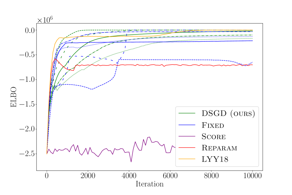
(a) temperature

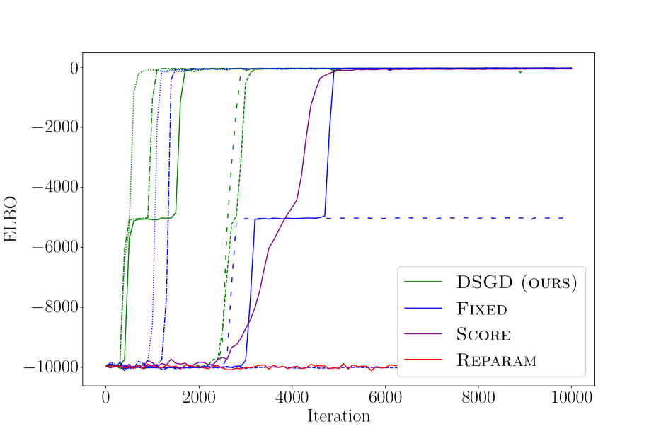
(b) xornet

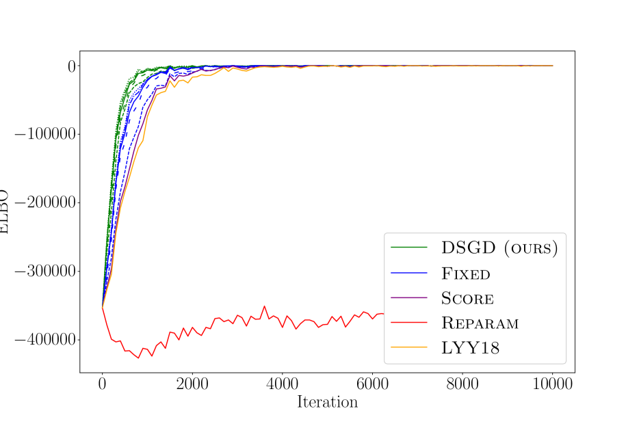
(c) random-walk

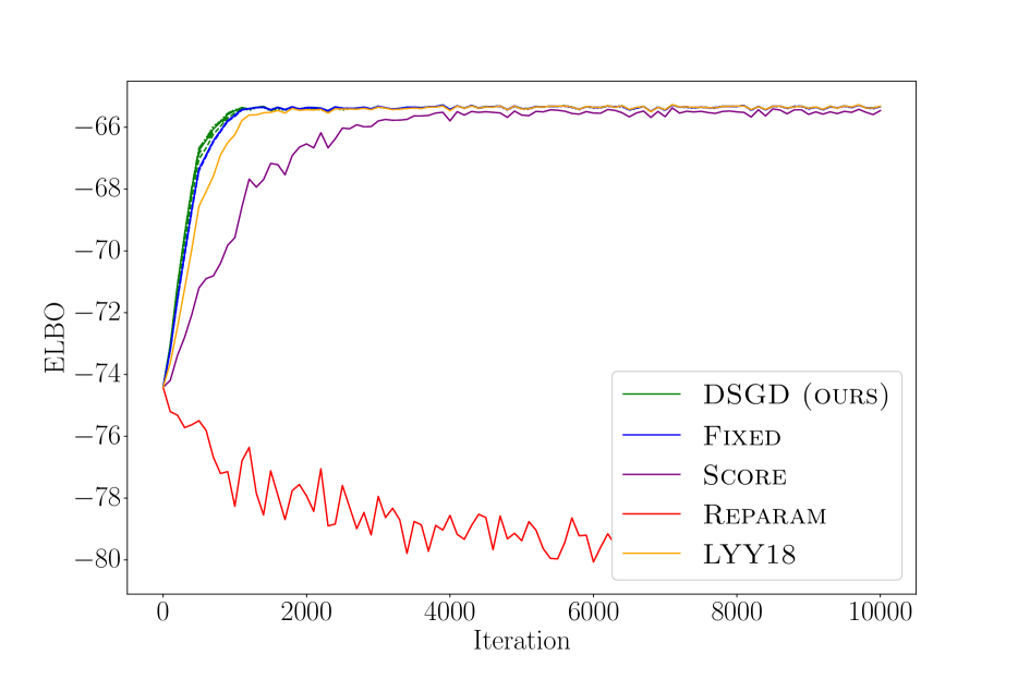
(d) cheating

Figure 2: ELBO trajectories for each model. A single colour is used for each estimator and the choice of $\eta=\eta_{4000}=0.06,0.1,0.14,0.18,0.22$ (which determines $\eta_{0}$) is represented by dashed, loosely dashed, solid, dash-dotted, dotted lines, respectively.

Experimental Set-Up.

The (Python) implementation is based on (Khajwal et al.,, 2023; Lee et al.,, 2018). We employ the jax library to provide automatic differentiation which is used to implement each of the above estimators for an arbitrary (probabilistic) program. The smoothed interpretation can be obtained automatically by (recursively) replacing conditionals $\mathbf{if}\,E_{1}<0\,\mathbf{then}\,E_{2}\,\mathbf{else}\,E_{3}$ with $\sigma_{\eta}(-E_{1})\cdot E_{2}+\sigma_{\eta}(E_{1})\cdot E_{3}$ in a preprocessing step. (We avoid a potential blowup by using an auxiliary variable for $E_{1}$.)

In view of Theorem 5.6, for DSGD we choose the accuracy coefficient schemes $\eta_{k}\coloneqq\eta_{0}/\sqrt{k}$ for $\eta_{0}>0$; due to the nesting of guards we use $\eta_{k}\coloneqq\eta_{0}\cdot k^{-0.2}$ for xornet. We compare (using the same line style) DSGD for different choices of $\eta_{0}$ to Fixed using the fixed accuracy coefficient corresponding to $\eta_{4000}$.

To enable a fair comparison to (Khajwal et al.,, 2023; Lee et al.,, 2018), we follow their set-up and use the state-of-the-art stochastic optimiser Adam with a step size of 0.001, except for xornet for which we use 0.01, for 10,000 iterations. For each iteration, we use $16$ Monte Carlo samples from the chosen estimator to compute the gradient. As in (Lee et al.,, 2018), the LYY18 estimator does not compute the boundary surface term exactly, but estimates it using a single subsample.

For every $100$ iterations, we take $1000$ samples of the estimator to estimate the current ELBO value and the variance of the gradient. Since the gradient is a vector, the variance is taken in two ways: averaging the component-wise variances and the variance of the L2 norm.

We separately benchmark each estimator by computing the number of iterations each can complete in a fixed time budget; the computational cost of each estimator is then estimated to be the reciprocal of this number. This then allows us to compute a set of work-normalised variances (Botev and Ridder,, 2017) for each estimator, which are the product of the computational cost and the variance.

Table 1: Mean of the final ELBO (the higher the better) for different random seeds and indicating error bars (the $\pm$ is one standard deviation).

(a) temperature

$\eta/\eta_{4000}$	DSGD (ours)	Fixed	Score	Reparam	LYY18
0.06	-76 $\pm$ 1	-624,250 $\pm$ 44,121
0.1	-84 $\pm$ 2	-425 $\pm$ 9	-2,611,479 $\pm$ 255,193	-706,729 $\pm$ 4,697	-17,502 $\pm$ 52,044
0.14	-15,476 $\pm$ 4,641	-121,932 $\pm$ 85,460

(b) xornet

$\eta/\eta_{4000}$	DSGD (ours)	Fixed	Score	Reparam
0.06	-3,530 $\pm$ 3,889	-5,522 $\pm$ 4,136
0.1	-33 $\pm$ 7	-2,029 $\pm$ 3,305	-553 $\pm$ 1,507	-9,984 $\pm$ 38
0.14	-27 $\pm$ 4	-2,028 $\pm$ 3,986

Table 2: Computational cost and work-normalised variances, all given as ratios with respect to the Score estimator (omitted since it would be all $1$s).

(a) temperature

Estimator	Cost	$\textrm{Avg}(V(.))$	$V(\|.\|_{2})$
DSGD (ours)	1.71	4.91e-11	2.54e-10
Fixed	1.71	2.84e-10	2.24e-09
Reparam	1.26	1.47e-08	1.94e-08
LYY18	9.61	1.05e-06	4.04e-05

(b) xornet

Estimator	Cost	$\textrm{Avg}(V(.))$	$V(\|.\|_{2})$
DSGD (ours)	1.74	6.21e-03	3.66e-02
Fixed	1.87	1.21e-02	5.43e-02
Reparam	0.388	8.34e-09	2.62e-09

(c) random-walk

Estimator	Cost	$\textrm{Avg}(V(.))$	$V(\|.\|_{2})$
DSGD (ours)	4.70	1.71e-01	2.61e-01
Fixed	4.70	9.50e-01	1.49
Reparam	2.17	8.63e-10	7.01e-10
LYY18	4.81	7.92	1.26e+01

(d) cheating

Estimator	Cost	$\textrm{Avg}(V(.))$	$V(\|.\|_{2})$
DSGD (ours)	1.52	2.31e-03	3.51e-03
Fixed	1.52	2.84e-03	4.64e-03
Reparam	9.36e-01	4.14e-19	1.16e-18
LYY18	2.59	4.27e-02	1.09e-01

Analysis of Results.

The ELBO trajectories as well as the data for computational cost and variance are presented Figs. 2 and 2 (additional models are covered in Appendix E). [dw]Besides, Table 1 lists the mean and standard deviation of the final ELBO across different seeds for the random number generator. Empirically, the bias of Reparam becomes evident and Score exhibits very high variance, resulting in slow convergence or even inferior results (Fig. 2(a)).

Whenever the LYY18 estimator is applicable, the trajectories for DSGD perform comparably, however DSGD attains orders of magnitude reduction in work-normalised variance (4 to 20,000 x).

Compared to Fixed, we observe that DSGD is more robust to the choice of (initial) accuracy coefficients (especially for temperature and xornet). Besides, there is a moderate improvement of variance (Table 2).

7 CONCLUDING REMARKS

We have proposed a variant of SGD, Diagonalisation Stochastic Gradient Descent, and shown provable correctness. Our approach is based on a smoothed interpretation of (possibly) discontinuous programs, which also yields unbiased gradient estimators. Crucially, asymptotically a stationary point of the original, unsmoothed problem is attained and a hyperparameter (accuracy of approximations) is tuned automatically. The correctness hinges on a careful analysis of the variance and a compatible scheme governing the accuracies. Notably, this purely depends on the (syntactic) structure of the program.

Our experimental evaluation demonstrates important advantages over the state of the art: significantly lower variance (score estimator), unbiasedness (reparametrisation estimator), simplicity, wider applicability and lower variance (unbiased correction thereof), as well as stability over the choice of (initial) accuracy coefficients (fixed smoothing).

Limitations and Future Directions.

Our analysis is asymptotic and focuses on stationary points, which leaves room for future research (convergence rates, avoidance of saddle points etc.).

Furthermore, we plan to explore methods adaptively tuning the accuracy coefficient rather than a priori fixing a scheme. Whilst the present work was primarily concerned with theoretical guarantees, we anticipate adaptive methods to outperform fixed schemes in practice (but likely without theoretical guarantees).

[dw]

Acknowledgements

This research is supported by the National Research Foundation, Singapore, under its RSS Scheme (NRF-RSS2022-009).

Checklist

1. For all models and algorithms presented, check if you include:

   1. A clear description of the mathematical setting, assumptions, algorithm, and/or model. [Yes/No/Not Applicable]

      We present the setting in Section 2 and state Assumptions 2.4 and 5.1. The DSGD algorithm is presented in Section 4.

   2. An analysis of the properties and complexity (time, space, sample size) of any algorithm. [Yes/No/Not Applicable]

      We prove an (asymptotic) convergence result Propositions 4.1 and 5.6.

   3. (Optional) Anonymized source code, with specification of all dependencies, including external libraries. [Yes/No/Not Applicable]

      The Python code is at https://github.com/domwagner/DSGD.git. The dependencies are jax, jaxlib, numpy, ipykernel, matplotlib.

2. For any theoretical claim, check if you include:

   1. Statements of the full set of assumptions of all theoretical results. [Yes/No/Not Applicable]

      See Assumptions 2.4 and 5.1.

   2. Complete proofs of all theoretical results. [Yes/No/Not Applicable]

      Proofs are presented in Appendices B, C and D.

   3. Clear explanations of any assumptions. [Yes/No/Not Applicable]

      We discuss Assumptions 2.4 and 5.2 in Sections 2 and 5.1, respectively.

3. For all figures and tables that present empirical results, check if you include:

   1. The code, data, and instructions needed to reproduce the main experimental results (either in the supplemental material or as a URL). [Yes/No/Not Applicable]

      The code is available at https://github.com/domwagner/DSGD.git. The experiements can be viewed and run in the jupyter notebook experiments.ipynb by running:

      jupyter notebook experiments.ipynb.

   2. All the training details (e.g., data splits, hyperparameters, how they were chosen). [Yes/No/Not Applicable]

      We present the details Sections 6 and 2 and closely follow the setup of Lee et al., (2018); Khajwal et al., (2023). In particular, the choice of the benchmarked hyperparameters $\eta=\eta_{4000}=0.06,0.1,0.14,0.18,0.22$ for Fig. 2 expands the range by Khajwal et al., (2023), who use $0.1,0.15,0.2$, and we uniformly split the range in steps of $0.04$.

   3. A clear definition of the specific measure or statistics and error bars (e.g., with respect to the random seed after running experiments multiple times). [Yes/No/Not Applicable]

      We describe our approach to compute the work-normalised variance and the computational cost in Section 6.

   4. A description of the computing infrastructure used. (e.g., type of GPUs, internal cluster, or cloud provider). [Yes/No/Not Applicable]

      We run our experiments on a MacBook Air (13-inch, 2017) with Intel HD Graphics 6000 1536 MB.

4. If you are using existing assets (e.g., code, data, models) or curating/releasing new assets, check if you include:

   1. Citations of the creator If your work uses existing assets. [Yes/No/Not Applicable]

   2. The license information of the assets, if applicable. [Yes/No/Not Applicable]

   3. New assets either in the supplemental material or as a URL, if applicable. [Yes/No/Not Applicable]

   4. Information about consent from data providers/curators. [Yes/No/Not Applicable]

   5. Discussion of sensible content if applicable, e.g., personally identifiable information or offensive content. [Yes/No/Not Applicable]

5. If you used crowdsourcing or conducted research with human subjects, check if you include:

   1. The full text of instructions given to participants and screenshots. [Yes/No/Not Applicable]

   2. Descriptions of potential participant risks, with links to Institutional Review Board (IRB) approvals if applicable. [Yes/No/Not Applicable]

   3. The estimated hourly wage paid to participants and the total amount spent on participant compensation. [Yes/No/Not Applicable]

Appendix A Supplementary Materials for Section 2

$F\in\mathrm{Expr}$ naturally defines a function $\mathbb{R}^{n}\to\mathbb{R}$, which we denote by $\llbracket F\rrbracket$:

$$\llbracket z_{j}\rrbracket(\mathbf{z}) \coloneqq z_{j}$$

$$\llbracket f(F_{1},\ldots,F_{k})\rrbracket(\mathbf{z}) \coloneqq f(\llbracket F_{1}\rrbracket(\mathbf{z}),\ldots,\llbracket F_{k}\rrbracket(\mathbf{z}))$$

$$\llbracket\mathbf{if}\,F<0\,\mathbf{then}\,G\,\mathbf{else}\,H\rrbracket(\mathbf{z}) \coloneqq\begin{cases}\llbracket G\rrbracket(\mathbf{z})&\text{if }\llbracket F\rrbracket(\mathbf{z})<0\\ \llbracket H\rrbracket(\mathbf{z})&\text{otherwise}\end{cases}$$

Table 3: Schwartz Distributions and their PDFs

distribution	pdf	support	parameters
normal	$\frac{1}{\sigma\sqrt{2\pi}}\exp\left(\frac{-(x-\mu)^{2}}{2\sigma^{2}}\right)$	$\mathbb{R}$	$\mu\in\mathbb{R},\sigma\in\mathbb{R}_{>0}$
half normal	$\frac{\sqrt{2}}{\sigma\sqrt{\pi}}\exp\left(\frac{-x^{2}}{2\sigma^{2}}\right)$	$\mathbb{R}_{\geq 0}$	$\sigma\in\mathbb{R}_{>0}$
exponential	$\lambda\cdot\exp(-\lambda x)$	$\mathbb{R}_{\geq 0}$	$\lambda\in\mathbb{R}_{>0}$
logistic	$\frac{\exp\left(-\frac{x-\mu}{s}\right)}{s\left(1+\exp\left(-\frac{x-\mu}{s}\right)\right)^{2}}$	$\mathbb{R}$	$\mu\in\mathbb{R},s\in\mathbb{R}_{>0}$

Appendix B Supplementary Materials for Section 3

The following immediately follows from a well-known result about exchanging differentiation and integration, which is a consequence of the dominated convergence theorem (Klenke,, 2014, Theorem 6.28):

Lemma B.1.

Let $\Theta\subseteq\mathbb{R}$ be open and $\mathbb{S}\subseteq\mathbb{R}^{n}$ be measurable. If $f:\Theta\times\mathbb{S}\to\mathbb{R}$ satisfies

1. for each $\theta\in\Theta$, $\mathbf{s}\mapsto f(\theta,\mathbf{s})$ is integrable

2. $f$ is differentiable

3. there exists an integrable $g:\mathbb{S}\to\mathbb{R}$ satisfying $|\frac{\partial f}{\partial\theta}(\theta,\mathbf{s})|\leq g(\mathbf{s})$ for all $(\theta,\mathbf{s})\in\Theta\times\mathbb{S}$.

then for all $\theta\in\Theta$, $\frac{\partial}{\partial\theta}\int_{\mathbb{S}}f(\theta,\mathbf{s})\mathop{}\!\mathrm{d}\mathbf{s}=\int_{\mathbb{S}}\frac{\partial f}{\partial\theta}(\theta,\mathbf{s})\mathop{}\!\mathrm{d}\mathbf{s}$.

Note that the second premise fails for the function $f$ in Example 1.1: for all $s\in\mathbb{R}$, $\frac{\partial f}{\partial\theta}(-s,s)$ does not exist.

See 3.1

Proof.

Let ${\boldsymbol{\theta}}\in{\boldsymbol{\Theta}}$. We apply Lemma B.1 to some ball ${\boldsymbol{\Theta}}^{\prime}\subseteq{\boldsymbol{\Theta}}$ around ${\boldsymbol{\theta}}$ and $(\mathbf{s},{\boldsymbol{\theta}})\mapsto\mathbf{\mathcal{D}}(\mathbf{s})\cdot\llbracket F\rrbracket_{\eta}({\boldsymbol{\phi}}_{\boldsymbol{\theta}}(\mathbf{s}))$. We have already seen the well-definedness (first premise) and the second is obvious (since $\llbracket F\rrbracket_{\eta}$ is a smoothing). For the third premise, we observe that for each $\eta>0$, $\frac{\partial(\llbracket F\rrbracket_{\eta}\circ{\boldsymbol{\phi}}_{(-)})}{\partial\theta_{i}}$ is bounded by a polynomial (using Assumption 2.4). Therefore, by Lemma B.2 (below) there exists a polynomial $p:\mathbb{R}^{n}\to\mathbb{R}$ satisfying $\frac{\partial(\llbracket F\rrbracket_{\eta}\circ{\boldsymbol{\phi}}_{(-)})}{\partial\theta_{i}}({\boldsymbol{\theta}},\mathbf{s})\leq|p(\mathbf{s})|$ for all $({\boldsymbol{\theta}},\mathbf{s})\in{\boldsymbol{\Theta}}^{\prime}\times\mathbb{R}^{n}$ and integrability of $\mathbf{\mathcal{D}}(\mathbf{s})\cdot p(\mathbf{s})$ follows with Lemma 2.3. ∎

Lemma B.2.

1. If $p:\mathbb{R}^{n}\to\mathbb{R}$ is a polynomial then there exists a polynomial $q$ such that for all $|x_{1}|\leq|x^{\prime}_{1}|,\ldots,|x_{n}|\leq|x_{n}^{\prime}|$, $|p(\mathbf{x})|\leq q(\mathbf{x}^{\prime})$.

2. If $f:{\boldsymbol{\Theta}}\times\mathbb{R}^{n}\to\mathbb{R}$ is bounded by a polynomial, where ${\boldsymbol{\Theta}}\subseteq\mathbb{R}^{m}$ is compact then there exists a polynomial $p:\mathbb{R}^{n}\to\mathbb{R}$ satisfying $|f({\boldsymbol{\theta}},\mathbf{x})|\leq p(\mathbf{x})$ for all $({\boldsymbol{\theta}},\mathbf{x})\in{\boldsymbol{\Theta}}\times\mathbb{R}^{n}$.

For example for $p(x_{1},x_{2})=x_{1}^{2}\cdot x_{2}-x_{2}$ the polynomial $x_{1}^{2}\cdot(x_{2}^{2}+1)+(x_{2}^{2}+1)$ satisfies this property. (The following proof yields $((x_{1}^{2}+1)^{2}+1)\cdot(x_{2}^{2}+1)+(x_{2}^{2}+1)$.) Besides, $p(\theta,x_{1},x_{2})=\theta\cdot x_{1}\cdot x_{2}-x_{2}$ is uniformly bounded by $2\cdot(x_{1}^{2}+1)\cdot(x_{2}^{2}+1)+(x_{2}^{2}+1)$ on $\Theta=(-2,1)$.

Proof.

1. If $p(\mathbf{x})=x_{i}$ then we can choose $q(\mathbf{x})\coloneqq(x_{i}^{2}+1)$ because for $|x_{i}|\leq|x^{\prime}_{i}|$, $|x_{i}|\leq|x_{i}^{\prime}|<(x_{i}^{\prime})^{2}+1$.

   If $p(\mathbf{x})=c$ for $c\in\mathbb{R}$ then we can choose $q(\mathbf{x})\coloneqq|c|$.

   Finally, suppose that $p_{1},p_{2},q_{1},q_{2}$ are polynomials such that for all $|\mathbf{x}|\leq|\mathbf{x}^{\prime}|$, $|p_{1}(\mathbf{x})|\leq q_{1}(\mathbf{x}^{\prime})$ and $|p_{2}(\mathbf{x})|\leq q_{2}(\mathbf{x}^{\prime})$. Then for all $|\mathbf{x}|\leq|\mathbf{x}^{\prime}|$,

   $$|p_{1}(\mathbf{x})+p_{2}(\mathbf{x})| \leq|p_{1}(\mathbf{x})|+|p_{2}(\mathbf{x})|\leq q_{1}(\mathbf{x}^{\prime})+q_{2}(\mathbf{x}^{\prime})$$

   $$|p_{1}(\mathbf{x})\cdot p_{2}(\mathbf{x})| \leq|p_{1}(\mathbf{x})|\cdot|p_{2}(\mathbf{x})|\leq q_{1}(\mathbf{x}^{\prime})\cdot q_{2}(\mathbf{x}^{\prime})$$

2. If $f:{\boldsymbol{\Theta}}\times\mathbb{R}^{n}\to\mathbb{R}$ is bounded by a polynomial then by the first part there exists $q:{\boldsymbol{\Theta}}\times\mathbb{R}^{n}\to\mathbb{R}$ such that for all $({\boldsymbol{\theta}},\mathbf{z}),({\boldsymbol{\theta}}^{\prime},\mathbf{z})\in{\boldsymbol{\Theta}}\times\mathbb{R}^{n}$ with $|{\boldsymbol{\theta}}|\leq|{\boldsymbol{\theta}}^{\prime}|$, $|f({\boldsymbol{\theta}},\mathbf{z})|\leq q({\boldsymbol{\theta}},\mathbf{z}^{\prime})$. Let $\theta_{i}^{*}\coloneqq\sup_{{\boldsymbol{\theta}}\in{\boldsymbol{\Theta}}}\theta_{i}<\infty$ (${\boldsymbol{\Theta}}$ is bounded) and $p(\mathbf{z})\coloneqq q(\mathbf{z},{\boldsymbol{\theta}}^{*})$. Finally, it suffices to note that for every $({\boldsymbol{\theta}},\mathbf{z})\in{\boldsymbol{\Theta}}\times\mathbb{R}^{n}$, $|f({\boldsymbol{\theta}},\mathbf{z})|\leq q({\boldsymbol{\theta}}^{*},\mathbf{z})=p(\mathbf{z})$. ∎

Appendix C Supplementary Materials for Section 4

See 4.1

Proof.

Let $L$ be the constant for Lipschitz smoothness in (D2). By Taylor’s theorem, ${\boldsymbol{\theta}}_{k},{\boldsymbol{\theta}}_{k+1}\in{\boldsymbol{\Theta}}$ and convexity of ${\boldsymbol{\Theta}}$,

$$\mathbb{E}_{\mathbf{s}_{k}\sim\mathbf{\mathcal{D}}}[g({\boldsymbol{\theta}}_{k+1})] \leq\mathbb{E}_{\mathbf{s}_{k}\sim\mathbf{\mathcal{D}}}\left[g({\boldsymbol{\theta}}_{k})-\gamma_{k}\cdot\langle\nabla_{\boldsymbol{\theta}}\,g({\boldsymbol{\theta}}_{k}),\nabla_{\boldsymbol{\theta}}\,f_{k}({\boldsymbol{\theta}}_{k},\mathbf{s}_{k})\rangle+\frac{\gamma_{k}^{2}}{2}\cdot L\cdot\|\nabla_{\boldsymbol{\theta}}\,f_{k}({\boldsymbol{\theta}}_{k},\mathbf{s}_{k})\|^{2}\right]$$

$$\leq g({\boldsymbol{\theta}}_{k})-\gamma_{k}\cdot\langle\nabla_{\boldsymbol{\theta}}\,g({\boldsymbol{\theta}}_{k}),\nabla_{\boldsymbol{\theta}}\,g_{k}({\boldsymbol{\theta}}_{k})\rangle+\frac{\gamma_{k}^{2}}{2}\cdot L\cdot V_{k}$$

using (D1) and (D3) in the second step. Hence,

$$\gamma_{k}\cdot\langle\nabla_{\boldsymbol{\theta}}\,g({\boldsymbol{\theta}}_{k}),\nabla_{\boldsymbol{\theta}}\,g_{k}({\boldsymbol{\theta}}_{k})\rangle\leq g({\boldsymbol{\theta}}_{k})-\mathbb{E}_{\mathbf{s}_{k}\sim\mathbf{\mathcal{D}}}[g({\boldsymbol{\theta}}_{k+1})]+\frac{\gamma_{k}^{2}}{2}\cdot L\cdot V_{k}$$

and thus,

$$\sum_{i=0}^{k-1}\gamma_{i}\cdot\mathbb{E}_{\mathbf{s}_{0},\ldots,\mathbf{s}_{k-1}\sim\mathbf{\mathcal{D}}}[\langle\nabla_{\boldsymbol{\theta}}\,g({\boldsymbol{\theta}}_{i}),\nabla_{\boldsymbol{\theta}}\,g_{i}({\boldsymbol{\theta}}_{i})\rangle] \leq g({\boldsymbol{\theta}}_{0})-\mathbb{E}[g({\boldsymbol{\theta}}_{k})]+L\cdot\sum_{i=0}^{k-1}\frac{\gamma_{i}^{2}}{2}\cdot V_{i}$$

By boundedness (D2), $g({\boldsymbol{\theta}}_{0})-\mathbb{E}[g({\boldsymbol{\theta}}_{k})]\leq c<\infty$ (for some $c>0$) and therefore due to Eq. 2 it follows:

$$\inf_{i\in\mathbb{N}}\mathbb{E}[\langle\nabla_{\boldsymbol{\theta}}\,g({\boldsymbol{\theta}}_{i}),\nabla_{\boldsymbol{\theta}}\,g_{i}({\boldsymbol{\theta}}_{i})\rangle]\leq\left(\sum_{i\in\mathbb{N}}\gamma_{i}\right)^{-1}\cdot\left(c+L\cdot\sum_{i\in\mathbb{N}}\frac{\gamma_{i}^{2}}{2}\cdot V_{i}\right)=0$$ (4)

By the same reasoning for all $i_{0}\in\mathbb{N}$, $\inf_{i\geq i_{0}}\mathbb{E}[\langle\nabla_{\boldsymbol{\theta}}\,g({\boldsymbol{\theta}}_{i}),\nabla_{\boldsymbol{\theta}}\,g_{i}({\boldsymbol{\theta}}_{i})\rangle]=0$ and therefore also $\liminf_{i\in\mathbb{N}}\mathbb{E}[\langle\nabla_{\boldsymbol{\theta}}\,g({\boldsymbol{\theta}}_{i}),\nabla_{\boldsymbol{\theta}}\,g_{i}({\boldsymbol{\theta}}_{i})\rangle]=0$.

Next, observe that

$$\|g({\boldsymbol{\theta}}_{i})\|^{2} =\langle\nabla_{\boldsymbol{\theta}}\,g({\boldsymbol{\theta}}_{i}),\nabla_{\boldsymbol{\theta}}\,g_{i}({\boldsymbol{\theta}}_{i})\rangle+\langle\nabla_{\boldsymbol{\theta}}\,g({\boldsymbol{\theta}}_{i}),\nabla_{\boldsymbol{\theta}}\,g({\boldsymbol{\theta}}_{i})-\nabla_{\boldsymbol{\theta}}\,g_{i}({\boldsymbol{\theta}}_{i})\rangle$$

$$\leq\langle\nabla_{\boldsymbol{\theta}}\,g({\boldsymbol{\theta}}_{i}),\nabla_{\boldsymbol{\theta}}\,g_{i}({\boldsymbol{\theta}}_{i})\rangle+\|\nabla_{\boldsymbol{\theta}}\,g({\boldsymbol{\theta}}_{i})\|\cdot\|\nabla_{\boldsymbol{\theta}}\,g({\boldsymbol{\theta}}_{i})-\nabla_{\boldsymbol{\theta}}\,g_{i}({\boldsymbol{\theta}}_{i})\|$$

and the right summand uniformly converges to $0$ because of Lipschitz continuity (D2) and the fact that $\|\nabla_{\boldsymbol{\theta}}\,g({\boldsymbol{\theta}}_{i})-\nabla_{\boldsymbol{\theta}}\,g_{i}({\boldsymbol{\theta}}_{i})\|$ does so (D4). Consequently,

$$\liminf_{i\in\mathbb{N}}\mathbb{E}\left[\|g({\boldsymbol{\theta}}_{i})\|^{2}\right]=0$$

Finally, this can only possibly hold if almost surely $\liminf_{i\in\mathbb{N}}\|g({\boldsymbol{\theta}}_{i})\|^{2}=0$. ∎

Appendix D Supplementary Materials for Section 5

The following can be viewed as an extension of Lemma 2.3(2) and is useful for Lemma D.3:

Lemma D.1.

If $f:{\boldsymbol{\Theta}}\times\mathbb{S}\to\mathbb{R}$ is continuous and satisfies

$$\sup_{({\boldsymbol{\theta}},\mathbf{z})\in{\boldsymbol{\Theta}}\times\mathbb{S}}\|\mathbf{z}\|^{n+3}\cdot|f({\boldsymbol{\theta}},\mathbf{z})|<\infty$$

then $\int_{\mathbb{S}}\sup_{{\boldsymbol{\theta}}\in{\boldsymbol{\Theta}}}|f({\boldsymbol{\theta}},\mathbf{z})|\mathop{}\!\mathrm{d}\mathbf{z}<\infty$.

Proof.

Let $g(\mathbf{z})\coloneqq\sup_{{\boldsymbol{\theta}}\in{\boldsymbol{\Theta}}}|f({\boldsymbol{\theta}},\mathbf{z})|$ and $U_{k}\coloneqq\mathbb{S}\cap[-k,k]^{n}$. Therefore,

$$\int_{\mathbb{S}}g(\mathbf{z})\mathop{}\!\mathrm{d}\mathbf{z}$$

$$=\int_{U_{1}}g(\mathbf{z})\mathop{}\!\mathrm{d}\mathbf{z}+\int_{\mathbb{S}\setminus U_{1}}g(\mathbf{z})\mathop{}\!\mathrm{d}\mathbf{z}$$

$$\leq 2^{n}\cdot\sup_{({\boldsymbol{\theta}},\mathbf{z})\in{\boldsymbol{\Theta}}\times U_{1}}|f({\boldsymbol{\theta}},\mathbf{z})|+\left(\sup_{({\boldsymbol{\theta}},\mathbf{z})\in{\boldsymbol{\Theta}}\times\mathbb{S}}\|\mathbf{z}\|^{n+3}\cdot f({\boldsymbol{\theta}},\mathbf{z})\right)\cdot\int_{\mathbb{S}\setminus U_{1}}\frac{1}{\|\mathbf{z}\|^{n+3}}\mathop{}\!\mathrm{d}\mathbf{z}$$

All the terms are finite because (NB if $\mathbf{z}\in\mathbb{S}\setminus U_{k}$ then $k\leq\|\mathbf{z}\|$)

$$\int_{\mathbb{S}\setminus U_{1}}\frac{1}{\|\mathbf{z}\|^{n+3}}\mathop{}\!\mathrm{d}\mathbf{z} =\sum_{k=1}^{\infty}\int_{U_{k+1}\setminus U_{k}}\frac{1}{\|\mathbf{z}\|^{n+3}}\mathop{}\!\mathrm{d}\mathbf{z}$$

$$\leq\sum_{k=1}^{\infty}\int_{U_{k+1}}\frac{1}{k^{n+3}}\mathop{}\!\mathrm{d}\mathbf{z}$$

$$\leq\sum_{k=1}^{\infty}\frac{(2k)^{n+1}}{k^{n+3}}\mathop{}\!\mathrm{d}\mathbf{z}$$

$$\leq 4^{n}\cdot\sum_{k=1}^{\infty}\frac{1}{k^{2}}\mathop{}\!\mathrm{d}\mathbf{z}<\infty\qed$$

Lemma D.2.

If $f:\mathbb{S}\to\mathbb{R}$, where $\mathbb{S}\subseteq\mathbb{R}^{n}$, is a Schwartz function, ${\boldsymbol{\phi}}_{(-)}:{\boldsymbol{\Theta}}\times\mathbb{R}^{n}\to\mathbb{R}^{n}$ satisfies Assumptions 2.4 and 5.2, and $p:\mathbb{R}^{n}\to\mathbb{R}$ a polynomial then

$$\int_{\mathbb{S}}\sup_{{\boldsymbol{\theta}}\in{\boldsymbol{\Theta}}}\left|f({\boldsymbol{\phi}}_{{\boldsymbol{\theta}}}^{-1}(\mathbf{z}))\cdot\det\mathbf{J}{\boldsymbol{\phi}}_{\boldsymbol{\theta}}^{-1}(\mathbf{z})\cdot p(\mathbf{z})\right|\mathop{}\!\mathrm{d}\mathbf{z}<\infty$$

Proof.

Since ${\boldsymbol{\phi}}_{(-)}$ satisfies Assumption 5.2, there exists $c>0$ such that $|\det\mathbf{J}{\boldsymbol{\phi}}_{\boldsymbol{\theta}}^{-1}(\mathbf{z})|\leq c$ and by Assumptions 2.4 and B.2 there exists a polynomial $q:\mathbb{R}^{n}\to\mathbb{R}$ satisfying

$$\left|\|{\boldsymbol{\phi}}_{\boldsymbol{\theta}}(\mathbf{s})\|^{n+3}+p({\boldsymbol{\phi}}_{\boldsymbol{\theta}}(\mathbf{s}))\right|\leq q(\mathbf{s})$$

for all $({\boldsymbol{\theta}},\mathbf{s})\in{\boldsymbol{\Theta}}\times\mathbb{S}$. Hence,

$$\sup_{({\boldsymbol{\theta}},\mathbf{z})\in{\boldsymbol{\Theta}}\times\mathbb{S}}\|\mathbf{z}\|^{n+3}\cdot\left|f({\boldsymbol{\phi}}_{{\boldsymbol{\theta}}}^{-1}(\mathbf{z}))\cdot\det\mathbf{J}{\boldsymbol{\phi}}_{\boldsymbol{\theta}}^{-1}(\mathbf{z})\cdot p(\mathbf{z})\right|$$

$$=\sup_{({\boldsymbol{\theta}},\mathbf{s})\in{\boldsymbol{\Theta}}\times\mathbb{S}}\|{\boldsymbol{\phi}}_{\boldsymbol{\theta}}(\mathbf{s})\|^{n+3}\cdot|f(\mathbf{s})|\cdot\underbrace{\left|\det\mathbf{J}{\boldsymbol{\phi}}_{\boldsymbol{\theta}}^{-1}({\boldsymbol{\phi}}_{\boldsymbol{\theta}}(\mathbf{s}))\right|}_{\leq c}\cdot|p({\boldsymbol{\phi}}_{\boldsymbol{\theta}}(\mathbf{s}))|$$

$$=c\cdot\sup_{\mathbf{s}\in\mathbb{S}}q(\mathbf{s})\cdot|f(\mathbf{s})|<\infty$$

by definition of Schwartz functions and the claim follows with Lemma D.1. ∎

Lemma D.3.

If $f:\mathbb{S}\to\mathbb{R}$ is a Schwartz function, ${\boldsymbol{\phi}}_{(-)}:{\boldsymbol{\Theta}}\times\mathbb{R}^{n}\to\mathbb{R}^{n}$ satisfies Assumptions 2.4 and 5.2, and $p:\mathbb{R}^{n}\to\mathbb{R}$ a polynomial then

$$\int_{\mathbb{S}}\sup_{{\boldsymbol{\theta}}\in{\boldsymbol{\Theta}}}\left|\frac{\partial f_{(-)}}{\partial\theta_{i}}({\boldsymbol{\theta}},\mathbf{z})\cdot p(\mathbf{z})\right|\mathop{}\!\mathrm{d}\mathbf{z} <\infty$$

$$\int_{\mathbb{S}}\sup_{{\boldsymbol{\theta}}\in{\boldsymbol{\Theta}}}\left|\frac{\partial f_{(-)}}{\partial z_{i}}({\boldsymbol{\theta}},\mathbf{z})\cdot p(\mathbf{z})\right|\mathop{}\!\mathrm{d}\mathbf{z} <\infty$$

$$\int_{\mathbb{S}}\sup_{{\boldsymbol{\theta}}\in{\boldsymbol{\Theta}}}\left|\frac{\partial^{2}f_{(-)}}{\partial\theta_{i}\partial\theta_{j}}({\boldsymbol{\theta}},\mathbf{z})\cdot p(\mathbf{z})\right|\mathop{}\!\mathrm{d}\mathbf{z} <\infty$$

where $f_{\boldsymbol{\theta}}(\mathbf{z})\coloneqq f({\boldsymbol{\phi}}_{{\boldsymbol{\theta}}}^{-1}(\mathbf{z}))\cdot|\det\mathbf{J}{\boldsymbol{\phi}}_{\boldsymbol{\theta}}^{-1}(\mathbf{z})|$.

Proof.

As for Lemma D.2, by Lemma D.1 it suffices to prove

$$\sup_{({\boldsymbol{\theta}},\mathbf{z})\in{\boldsymbol{\Theta}}\times\mathbb{S}}\|\mathbf{z}\|^{n+2}\cdot\left|\frac{\partial f_{(-)}}{\partial\theta_{i}}\cdot p(\mathbf{z})\right|$$

for the first claim. Note that

$$0=\mathbf{J}_{\theta_{i}}({\boldsymbol{\phi}}_{\boldsymbol{\theta}}\circ{\boldsymbol{\phi}}_{\boldsymbol{\theta}}^{-1})(\mathbf{z})=\mathbf{J}_{\theta_{i}}{\boldsymbol{\phi}}_{\boldsymbol{\theta}}({\boldsymbol{\phi}}_{\boldsymbol{\theta}}^{-1}(\mathbf{z}))+\mathbf{J}_{\mathbf{s}}{\boldsymbol{\phi}}_{\boldsymbol{\theta}}({\boldsymbol{\phi}}_{\boldsymbol{\theta}}^{-1}(\mathbf{z}))\cdot\mathbf{J}_{\theta_{i}}{\boldsymbol{\phi}}_{\boldsymbol{\theta}}^{-1}(\mathbf{z})$$

and hence,

$$\mathbf{J}_{\theta_{i}}{\boldsymbol{\phi}}_{\boldsymbol{\theta}}^{-1}(\mathbf{z}) =-\left(\mathbf{J}_{\mathbf{s}}{\boldsymbol{\phi}}_{\boldsymbol{\theta}}({\boldsymbol{\phi}}_{\boldsymbol{\theta}}^{-1}(\mathbf{z}))\right)^{-1}\cdot\mathbf{J}_{\theta_{i}}{\boldsymbol{\phi}}_{\boldsymbol{\theta}}({\boldsymbol{\phi}}_{\boldsymbol{\theta}}^{-1}(\mathbf{z}))$$

$$=-\frac{1}{|\det\mathbf{J}{\boldsymbol{\phi}}_{\boldsymbol{\theta}}({\boldsymbol{\phi}}_{\boldsymbol{\theta}}^{-1}(\mathbf{z}))|}\cdot\mathrm{adj}(\mathbf{J}{\boldsymbol{\phi}}_{\boldsymbol{\theta}}({\boldsymbol{\phi}}_{\boldsymbol{\theta}}^{-1}(\mathbf{z})))\cdot\mathbf{J}_{\theta_{i}}{\boldsymbol{\phi}}_{\boldsymbol{\theta}}({\boldsymbol{\phi}}_{\boldsymbol{\theta}}^{-1}(\mathbf{z}))$$

$$=-\frac{1}{|\det\mathbf{J}{\boldsymbol{\phi}}_{\boldsymbol{\theta}}({\boldsymbol{\phi}}_{\boldsymbol{\theta}}^{-1}(\mathbf{z}))|}\cdot\mathbf{g}({\boldsymbol{\theta}},{\boldsymbol{\phi}}_{\boldsymbol{\theta}}^{-1}(\mathbf{z}))$$

for a suitable function $\mathbf{g}:{\boldsymbol{\Theta}}\times\mathbb{R}^{n}\to\mathbb{R}^{n}$ bounded by polynomials (component-wise). Therefore,

$$\frac{\partial(f\circ{\boldsymbol{\phi}}_{(-)}^{-1})}{\partial\theta_{i}}(\mathbf{z}) =\nabla f({\boldsymbol{\phi}}_{\boldsymbol{\theta}}^{-1}(\mathbf{z}))\cdot\mathbf{J}_{\theta_{i}}{\boldsymbol{\phi}}_{\boldsymbol{\theta}}^{-1}(\mathbf{z})$$

$$=\frac{\nabla f({\boldsymbol{\phi}}_{\boldsymbol{\theta}}^{-1}(\mathbf{z}))\cdot\mathbf{g}({\boldsymbol{\theta}},{\boldsymbol{\phi}}_{\boldsymbol{\theta}}^{-1}(\mathbf{z}))}{|\det\mathbf{J}{\boldsymbol{\phi}}_{\boldsymbol{\theta}}({\boldsymbol{\phi}}_{\boldsymbol{\theta}}^{-1}(\mathbf{z}))|}$$

By Assumption 5.2, there exists $c>0$ satisfying

$$\frac{1}{|\det\mathbf{J}{\boldsymbol{\phi}}_{\boldsymbol{\theta}}({\boldsymbol{\phi}}_{\boldsymbol{\theta}}^{-1}(\mathbf{z}))|}=|\det\mathbf{J}{\boldsymbol{\phi}}^{-1}_{\boldsymbol{\theta}}(\mathbf{z})| \leq c$$

for all ${\boldsymbol{\theta}}\in{\boldsymbol{\Theta}}$ and $\mathbf{z}\in\mathbb{S}$. Consequently,

$$\sup_{({\boldsymbol{\theta}},\mathbf{z})\in{\boldsymbol{\Theta}}\times\mathbb{S}}\left|\|\mathbf{z}\|^{n+2}\cdot\frac{\partial(f\circ{\boldsymbol{\phi}}^{-1}_{(-)})}{\partial\theta_{i}}(\mathbf{z})\cdot\det\mathbf{J}{\boldsymbol{\phi}}^{-1}_{\boldsymbol{\theta}}(\mathbf{z})\cdot p(\mathbf{z})\right|$$

$$\leq c^{2}\cdot\sup_{({\boldsymbol{\theta}},\mathbf{s})\in{\boldsymbol{\Theta}}\times\mathbb{S}}\left|\|{\boldsymbol{\phi}}_{\boldsymbol{\theta}}(\mathbf{s})\|^{n+2}\cdot(\nabla f(\mathbf{s})\cdot\mathbf{g}({\boldsymbol{\theta}},\mathbf{s}))\cdot p({\boldsymbol{\phi}}_{\boldsymbol{\theta}}(\mathbf{s}))\right|<\infty$$

because ${\boldsymbol{\phi}}_{\boldsymbol{\theta}}(\mathbf{s})$, $\mathbf{g}({\boldsymbol{\theta}},\mathbf{s})$ and $p({\boldsymbol{\phi}}_{\boldsymbol{\theta}}(\mathbf{s}))$ are uniformly bounded by polynomials independent of ${\boldsymbol{\theta}}$ (by Lemma B.2) and derivatives of Schwartz functions are Schwartz functions, too.

Likewise, note that

$$|\det\mathbf{J}{\boldsymbol{\phi}}_{\boldsymbol{\theta}}^{-1}(\mathbf{z})|=\frac{1}{|\det\mathbf{J}{\boldsymbol{\phi}}_{\boldsymbol{\theta}}({\boldsymbol{\phi}}_{\boldsymbol{\theta}}^{-1}(\mathbf{z}))|}=\frac{1}{h({\boldsymbol{\theta}},{\boldsymbol{\phi}}_{\boldsymbol{\theta}}^{-1}(\mathbf{z}))}$$

for a function $h:{\boldsymbol{\Theta}}\times\mathbb{R}^{n}\to\mathbb{R}$, the partial derivatives of which are bounded by polynomials and which we can assume by Assumption 2.4 w.l.o.g. to be positive (and greater than the constant $c$ above).

Thus,

$$\frac{\partial}{\partial\theta_{i}}\det\mathbf{J}{\boldsymbol{\phi}}_{\boldsymbol{\theta}}^{-1}(\mathbf{z}) =\frac{\partial}{\partial\theta_{i}}\frac{1}{h({\boldsymbol{\theta}},{\boldsymbol{\phi}}_{\boldsymbol{\theta}}^{-1}(\mathbf{z}))}$$

$$=-\frac{\frac{\partial h}{\partial\theta_{i}}({\boldsymbol{\theta}},{\boldsymbol{\phi}}_{\boldsymbol{\theta}}^{-1}(\mathbf{z}))+\nabla_{\mathbf{s}}h({\boldsymbol{\theta}},{\boldsymbol{\phi}}_{\boldsymbol{\theta}}^{-1}(\mathbf{z}))\cdot\mathbf{J}_{\theta_{i}}{\boldsymbol{\phi}}_{\boldsymbol{\theta}}^{-1}(\mathbf{z})}{\left(h({\boldsymbol{\theta}},{\boldsymbol{\phi}}_{\boldsymbol{\theta}}^{-1}(\mathbf{z}))\right)^{2}}$$

$$=-\frac{\frac{\partial h}{\partial\theta_{i}}({\boldsymbol{\theta}},{\boldsymbol{\phi}}_{\boldsymbol{\theta}}^{-1}(\mathbf{z}))}{\underbrace{\left(h({\boldsymbol{\theta}},{\boldsymbol{\phi}}_{\boldsymbol{\theta}}^{-1}(\mathbf{z}))\right)^{2}}_{|\det\mathbf{J}{\boldsymbol{\phi}}^{-1}_{\boldsymbol{\theta}}(\mathbf{z})|^{-2}}}-\frac{\nabla_{\mathbf{s}}h({\boldsymbol{\theta}},{\boldsymbol{\phi}}_{\boldsymbol{\theta}}^{-1}(\mathbf{z}))\cdot\mathbf{g}({\boldsymbol{\theta}},{\boldsymbol{\phi}}_{\boldsymbol{\theta}}^{-1}(\mathbf{z}))}{\underbrace{\left(h({\boldsymbol{\theta}},{\boldsymbol{\phi}}_{\boldsymbol{\theta}}^{-1}(\mathbf{z}))\right)^{3}}_{|\det\mathbf{J}{\boldsymbol{\phi}}^{-1}_{\boldsymbol{\theta}}(\mathbf{z})|^{-3}}}$$

to show

$$\sup_{({\boldsymbol{\theta}},\mathbf{z})\in{\boldsymbol{\Theta}}\times\mathbb{S}}\left|\|\mathbf{z}\|^{n+2}\cdot f({\boldsymbol{\phi}}_{\boldsymbol{\theta}}^{-1}(\mathbf{z}))\cdot\frac{\partial}{\partial\theta_{i}}\det\mathbf{J}{\boldsymbol{\phi}}^{-1}_{\boldsymbol{\theta}}(\mathbf{z})\cdot p(\mathbf{z})\right|<\infty$$

The same insights can be used to show the second and third bounds. ∎

Corollary D.4 (Lipschitz Smoothness).

If $F\in\mathrm{Expr}$ then the function

$${\boldsymbol{\theta}}\mapsto\mathbb{E}_{\mathbf{s}\sim\mathbf{\mathcal{D}}}[\llbracket F\rrbracket({\boldsymbol{\phi}}_{\boldsymbol{\theta}}(\mathbf{s}))]$$

is Lipschitz smooth.

In the same manner we can prove the other (simpler) obligations of (D2).

D.1 Supplementary Materials for Section 5.1

See 5.4

Proof.

Let $p:\mathbb{R}^{n}\to\mathbb{R}$ be a polynomial bound to $\llbracket F\rrbracket_{\eta}$ and $\llbracket F\rrbracket$ and let $\epsilon>0$. We focus on the second result (the first is analogous). We define

$$c \coloneqq\int_{\mathbb{S}}\left|\sup_{{\boldsymbol{\theta}}\in{\boldsymbol{\Theta}}}\frac{\partial\mathbf{\mathcal{D}}_{(-)}}{\partial\theta_{i}}({\boldsymbol{\theta}},\mathbf{z})\right|\mathop{}\!\mathrm{d}\mathbf{z}$$

$$U_{k} \coloneqq\left\{\mathbf{z}\in\mathbb{R}^{n}\mid|f_{\eta}(\mathbf{z})-f(\mathbf{z})|>\frac{\epsilon}{2c}\text{ for some }0<\eta<\frac{1}{k}\right\}$$

$$\mu(U) \coloneqq\int_{U}p(\mathbf{z})\cdot\sup_{{\boldsymbol{\theta}}\in{\boldsymbol{\Theta}}}\left|\frac{\partial\mathbf{\mathcal{D}}_{(-)}}{\partial\theta_{i}}({\boldsymbol{\theta}},\mathbf{z})\right|\mathop{}\!\mathrm{d}\mathbf{z}$$

which is a finite measure by Lemma D.3. Note that $(U_{k})_{k\in\mathbb{N}}$ is a non-increasing sequence of sets and $\bigcap_{k\in\mathbb{N}}U_{k}$ is negligible. Hence, by continuity from above (of $\mu$) there exists $k$ such that $\mu(U_{k})<\frac{\epsilon}{4}$. Finally, it suffices to observe that for $0<\eta<\frac{1}{k}$ and ${\boldsymbol{\theta}}\in{\boldsymbol{\Theta}}$:

$$\left|\frac{\partial}{\partial\theta_{i}}\mathbb{E}_{\mathbf{s}\sim\mathbf{\mathcal{D}}}[\llbracket F\rrbracket_{\eta}({\boldsymbol{\phi}}_{\boldsymbol{\theta}}(\mathbf{s}))]-\frac{\partial}{\partial\theta_{i}}\mathbb{E}_{\mathbf{s}\sim\mathbf{\mathcal{D}}}[\llbracket F\rrbracket({\boldsymbol{\phi}}_{\boldsymbol{\theta}}(\mathbf{s}))]\right|$$

$$=\left|\frac{\partial}{\partial\theta_{i}}\mathbb{E}_{\mathbf{z}\sim\mathbf{\mathcal{D}}_{\boldsymbol{\theta}}}[\llbracket F\rrbracket_{\eta}(\mathbf{z})]-\frac{\partial}{\partial\theta_{i}}\mathbb{E}_{\mathbf{z}\sim\mathbf{\mathcal{D}}_{\boldsymbol{\theta}}}[\llbracket F\rrbracket(\mathbf{z})]\right|$$

$$\leq\int_{\mathbb{S}}\left|\frac{\partial\mathbf{\mathcal{D}}_{(-)}}{\partial\theta_{i}}({\boldsymbol{\theta}},\mathbf{z})\right|\cdot|\llbracket F\rrbracket_{\eta}(\mathbf{z})-\llbracket F\rrbracket(\mathbf{z})|\mathop{}\!\mathrm{d}\mathbf{z}$$

$$\leq\int_{U_{k}}\left|\frac{\partial\mathbf{\mathcal{D}}_{(-)}}{\partial\theta_{i}}({\boldsymbol{\theta}},\mathbf{z})\right|\cdot|\llbracket F\rrbracket_{\eta}(\mathbf{z})-\llbracket F\rrbracket(\mathbf{z})|\mathop{}\!\mathrm{d}\mathbf{z}$$

$$\qquad+\int_{\mathbb{S}\setminus U_{k}}\left|\frac{\partial\mathbf{\mathcal{D}}_{(-)}}{\partial\theta_{i}}({\boldsymbol{\theta}},\mathbf{z})\right|\cdot|\llbracket F\rrbracket_{\eta}(\mathbf{z})-\llbracket F\rrbracket(\mathbf{z})|\mathop{}\!\mathrm{d}\mathbf{z}$$

$$\leq 2\cdot\int_{U_{k}}\left|\frac{\partial\mathbf{\mathcal{D}}_{(-)}}{\partial\theta_{i}}({\boldsymbol{\theta}},\mathbf{z})\right|\cdot p(\mathbf{z})\mathop{}\!\mathrm{d}\mathbf{z}+\int_{\mathbb{S}\setminus U_{k}}\left|\frac{\partial\mathbf{\mathcal{D}}_{(-)}}{\partial\theta_{i}}({\boldsymbol{\theta}},\mathbf{z})\right|\cdot\frac{\epsilon}{2c}\mathop{}\!\mathrm{d}\mathbf{z}$$

$$\leq 2\cdot\mu(U_{k})+\frac{\epsilon}{2c}\cdot\int_{\mathbb{S}}\left|\frac{\partial\mathbf{\mathcal{D}}_{(-)}}{\partial\theta_{i}}({\boldsymbol{\theta}},\mathbf{z})\right|\mathop{}\!\mathrm{d}\mathbf{z}$$

$$\leq\epsilon\qed$$

Uniform convergence may fail if ${\boldsymbol{\Theta}}\subseteq\mathbb{R}^{m}$ is not compact:

Example D.5.

Let ${\boldsymbol{\Theta}}\coloneqq\mathbb{R}\times\mathbb{R}_{>0}$. $\mathbb{E}_{z\sim\mathcal{N}(\theta_{1},\theta_{2})}[\sigma_{\eta}(z)]$ does not converge uniformly to $\mathbb{E}_{z\sim\mathcal{N}(\theta_{1},\theta_{2})}[[z\geq 0]]$: Suppose $\eta>0$. There exists $\delta>0$ such that $\sigma_{\eta}(\delta)=0.6$. Define $\theta_{1}\coloneqq\theta_{2}\coloneqq\frac{\delta}{2}$. Now, it suffices to note that

$$\mathbb{E}_{z\sim\mathcal{N}(\theta_{1},\theta_{2})}[[z\geq 0]] \geq\int_{\theta_{1}-\theta_{2}}^{\infty}\mathcal{N}(z\mid\theta_{1},\theta_{2})\mathop{}\!\mathrm{d}z\geq 0.83$$

$$\mathbb{E}_{z\sim\mathcal{N}(\theta_{1},\theta_{2})}[\sigma_{\eta}(z)] \leq 0.5\int_{-\infty}^{\theta_{1}-\theta_{2}}\mathcal{N}(z\mid\theta_{1},\theta_{2})\mathop{}\!\mathrm{d}z+0.6\int_{\theta_{1}-\theta_{2}}^{\theta_{1}+\theta_{2}}\mathcal{N}(z\mid\theta_{1},\theta_{2})\mathop{}\!\mathrm{d}z+\int_{\theta_{1}+\theta_{2}}^{\infty}\mathcal{N}(z\mid\theta_{1},\theta_{2})\mathop{}\!\mathrm{d}z$$

$$\leq 0.5\cdot 0.16+0.6\cdot 0.69+0.16=0.654$$

D.2 Supplementary Materials for Section 5.2

Now, exploiting the chain rule and Assumption 2.4, it is straightforward to show inductively that for $F\in\mathrm{Expr}_{\ell}$,

Lemma D.6.

If $F\in\mathrm{Expr}_{\ell}$ there exists a polynomial $p:\mathbb{R}^{n}\to\mathbb{R}$ such that for all $\eta>0$ and $\mathbf{z}\in\mathbb{R}^{n}$,

$$\left|\frac{\partial\llbracket F\rrbracket_{\eta}}{\partial z_{i}}(\mathbf{z})\right|\leq|\sigma_{\eta}^{\prime}|^{\ell}\cdot p(\mathbf{z})$$

(By $|\sigma_{\eta}^{\prime}|$ we mean $\sup_{y\in\mathbb{R}}|\sigma_{\eta}^{\prime}(y)|$.)

Lemma D.7.

Let $F\in\mathrm{Expr}_{\ell}$, $f:\mathbb{S}\to\mathbb{R}$ be a non-negative Schwartz function, where $\mathbb{S}=U_{1}\times\cdots\times U_{n}$ and $U_{1},\ldots,U_{n}\in\{\mathbb{R},\mathbb{R}_{\geq 0}\}$, and $p$ be a non-negative polynomial. For all $1\leq i\leq n$ there exists $c>0$ such that for all [dw]$0<\eta\leq 1$,

$$\int_{\mathbb{S}}f_{\boldsymbol{\theta}}(\mathbf{z})\cdot p(\mathbf{z})\cdot\left|\frac{\partial^{2}\llbracket F\rrbracket_{\eta}}{\partial z_{i}^{2}}(\mathbf{z})\right|\mathop{}\!\mathrm{d}\mathbf{z} <c\cdot\eta^{-\ell}$$

$$\int_{\mathbb{S}}f_{\boldsymbol{\theta}}(\mathbf{z})\cdot p(\mathbf{z})\cdot\left|\frac{\partial\llbracket F\rrbracket_{\eta}}{\partial z_{i}}(\mathbf{z})\right|^{2}\mathop{}\!\mathrm{d}\mathbf{z} <c\cdot\eta^{-\ell}$$

where $f_{\boldsymbol{\theta}}\coloneqq f({\boldsymbol{\phi}}_{\boldsymbol{\theta}}^{-1}(\mathbf{z}))\cdot|\det\mathbf{J}{\boldsymbol{\phi}}_{\boldsymbol{\theta}}^{-1}(\mathbf{z})|$.

Proof.

Note that $f_{\boldsymbol{\theta}}$ is differentiable and non-negative. To simplify notation, we assume that $\mathbb{S}=\mathbb{R}^{n}$. (Otherwise the proof is similar, exploiting Lemma D.6.) Besides, it suffices to establish the first bound. To see that the second is a consequence of the first, we use integration by parts

$$\int f_{\boldsymbol{\theta}}(\mathbf{z})\cdot p(\mathbf{z})\cdot\left(\frac{\partial\llbracket F\rrbracket_{\eta}}{\partial z_{i}}(\mathbf{z})\right)^{2}\mathop{}\!\mathrm{d}\mathbf{z}$$

$$=\int\int\left(f_{\boldsymbol{\theta}}(\mathbf{z})\cdot p(\mathbf{z})\cdot\frac{\partial\llbracket F\rrbracket_{\eta}}{\partial z_{i}}(\mathbf{z})\right)\cdot\frac{\partial\llbracket F\rrbracket_{\eta}}{\partial z_{i}}(\mathbf{z})\mathop{}\!\mathrm{d}z_{j}\mathop{}\!\mathrm{d}\mathbf{z}_{-j}$$

$$=\int\underbrace{\left[f_{\boldsymbol{\theta}}(\mathbf{z})\cdot p(\mathbf{z})\cdot\frac{\partial\llbracket F\rrbracket_{\eta}}{\partial z_{i}}(\mathbf{z})\cdot\llbracket F\rrbracket_{\eta}(\mathbf{z})\right]^{\infty}_{-\infty}}_{=0}\mathop{}\!\mathrm{d}\mathbf{z}_{-j}$$

$$\qquad-\int\frac{\partial}{\partial z_{i}}\left(f_{\boldsymbol{\theta}}(\mathbf{z})\cdot p(\mathbf{z})\cdot\frac{\partial\llbracket F\rrbracket_{\eta}}{\partial z_{i}}(\mathbf{z})\right)\cdot\llbracket F\rrbracket_{\eta}(\mathbf{z})\mathop{}\!\mathrm{d}\mathbf{z}$$

where $\mathbf{z}_{-j}$ is $z_{1},\ldots,z_{j-1},z_{j+1},\ldots,j_{n}$, because by Lemma D.2, for fixed $\eta>0$ and $\mathbf{z}_{-j}$,

$$\lim_{z_{j}\to\pm\infty}f_{\boldsymbol{\theta}}(\mathbf{z})\cdot\underbrace{p(\mathbf{z})\cdot\frac{\partial\llbracket F\rrbracket_{\eta}}{\partial z_{i}}(\mathbf{z})\cdot\llbracket F\rrbracket_{\eta}(\mathbf{z})}_{\text{bounded by polynomial}}$$

We continue bounding:

$$-\int\frac{\partial}{\partial z_{i}}\left(f_{\boldsymbol{\theta}}(\mathbf{z})\cdot p(\mathbf{z})\cdot\frac{\partial\llbracket F\rrbracket_{\eta}}{\partial z_{i}}(\mathbf{z})\right)\cdot\llbracket F\rrbracket_{\eta}(\mathbf{z})\mathop{}\!\mathrm{d}\mathbf{z}$$

$$=-\int\frac{\partial f_{(-)}}{\partial z_{i}}({\boldsymbol{\theta}},\mathbf{z})\cdot p(\mathbf{z})\cdot\frac{\partial\llbracket F\rrbracket_{\eta}}{\partial z_{i}}(\mathbf{z})\cdot\llbracket F\rrbracket_{\eta}(\mathbf{z})\mathop{}\!\mathrm{d}\mathbf{z}$$

$$\qquad-\int f_{\boldsymbol{\theta}}(\mathbf{z})\cdot\frac{\partial p}{\partial z_{i}}(\mathbf{z})\cdot\frac{\partial\llbracket F\rrbracket_{\eta}}{\partial z_{i}}(\mathbf{z})\cdot\llbracket F\rrbracket_{\eta}(\mathbf{z})\mathop{}\!\mathrm{d}\mathbf{z}$$

$$\qquad-\int f_{\boldsymbol{\theta}}(\mathbf{z})\cdot p(\mathbf{z})\cdot\frac{\partial^{2}\llbracket F\rrbracket_{\eta}}{\partial z^{2}_{i}}(\mathbf{z})\cdot\llbracket F\rrbracket_{\eta}(\mathbf{z})\mathop{}\!\mathrm{d}\mathbf{z}$$

$$\leq\eta^{-\ell}\cdot\int\sup_{{\boldsymbol{\theta}}\in{\boldsymbol{\Theta}}}\left|\frac{\partial f_{(-)}}{\partial z_{i}}({\boldsymbol{\theta}},\mathbf{z})\cdot p_{1}(\mathbf{z})\right|\mathop{}\!\mathrm{d}\mathbf{z}$$

$$\qquad+\eta^{-\ell}\cdot\int\sup_{{\boldsymbol{\theta}}\in{\boldsymbol{\Theta}}}\left|f_{\boldsymbol{\theta}}(\mathbf{z})\cdot p_{2}(\mathbf{z})\right|\mathop{}\!\mathrm{d}\mathbf{z}$$

$$\qquad+\int f_{\boldsymbol{\theta}}(\mathbf{z})\cdot p_{3}(\mathbf{z})\cdot\left|\frac{\partial^{2}\llbracket F\rrbracket_{\eta}}{\partial z^{2}_{i}}(\mathbf{z})\right|$$

for suitable polynomial bounds $p_{1},p_{2},p_{3}:\mathbb{R}^{n}\to\mathbb{R}$ (which exist due to the fact that $\frac{\partial p}{\partial z_{i}}$ is a polynomial, Items 1 and D.6) and the second inequality follows with Lemma D.3.

We prove the claim by induction on the definition of $\mathrm{Expr}_{\ell}$:

• For $z_{j}\in\mathrm{Expr}_{0}$ and $F\in\mathrm{Expr}_{\ell+1}$ due to $F\in\mathrm{Expr}_{\ell}$ the claim is obvious.

• For $g(F_{1},\ldots,F_{k})\in\mathrm{Expr}_{\ell}$ because $F_{1},\ldots,f_{k}\in\mathrm{Expr}_{\ell}$,

  $$\int f_{\boldsymbol{\theta}}(\mathbf{z})\cdot p(\mathbf{z})\cdot\left|\frac{\partial^{2}(g\circ\langle\llbracket F_{1}\rrbracket_{\eta},\ldots,\llbracket F_{k}\rrbracket_{\eta}\rangle)}{\partial z_{i}^{2}}(\mathbf{z})\right|\mathop{}\!\mathrm{d}\mathbf{z}$$

  $$\leq\sum_{1\leq j,j^{\prime}\leq k}\int f_{\boldsymbol{\theta}}(\mathbf{z})\cdot p(\mathbf{z})\cdot\left|\frac{\partial^{2}g}{\partial y_{j}\partial y_{j^{\prime}}}(\llbracket F_{1}\rrbracket_{\eta}(\mathbf{z}),\ldots,\llbracket F_{k}\rrbracket_{\eta}(\mathbf{z}))\cdot\frac{\partial\llbracket F_{j}\rrbracket_{\eta}}{\partial z_{i}}(\mathbf{z})\cdot\frac{\partial\llbracket F_{j^{\prime}}\rrbracket_{\eta}}{\partial z_{i}}(\mathbf{z})\right|\mathop{}\!\mathrm{d}\mathbf{z}$$

  $$\qquad+\sum_{1\leq j\leq k}\int f_{\boldsymbol{\theta}}(\mathbf{z})\cdot p(\mathbf{z})\cdot\left|\frac{\partial g}{\partial y_{j}}(\llbracket F_{1}\rrbracket_{\eta}(\mathbf{z}),\ldots,\llbracket F_{k}\rrbracket_{\eta}(\mathbf{z}))\cdot\frac{\partial^{2}\llbracket F_{j}\rrbracket_{\eta}}{\partial^{2}z_{i}}(\mathbf{z})\right|\mathop{}\!\mathrm{d}\mathbf{z}$$

  By Assumption 2.4, $\frac{\partial g}{\partial y_{j}}(g_{\eta}^{(1)}(\mathbf{z}),\ldots,g_{\eta}^{(\ell)}(\mathbf{z}))$ is bounded by a polynomial. Therefore the second summand can be bounded by the inductive hypothesis. For the first, again by Assumption 2.4, we can bound

  $$p(\mathbf{z})\cdot\left|\frac{\partial^{2}g}{\partial y_{j}\partial y_{j^{\prime}}}(g_{\eta}^{(1)}(\mathbf{z}),\ldots,g_{\eta}^{(\ell)}(\mathbf{z}))\right|\leq p_{1}(\mathbf{z})$$

  for a (non-negative) polynomial $p_{1}$, apply the Cauchy-Schwarz inequality and apply the inductive hypothesis to

  $$\int f_{\boldsymbol{\theta}}(\mathbf{z})\cdot p_{1}(\mathbf{z})\cdot\left|\frac{\partial\llbracket F_{j}\rrbracket_{\eta}}{\partial z_{i}}(\mathbf{z})\right|^{2}\mathop{}\!\mathrm{d}\mathbf{z} \int f_{\boldsymbol{\theta}}(\mathbf{z})\cdot p_{1}(\mathbf{z})\cdot\left|\frac{\partial\llbracket F_{j^{\prime}}\rrbracket_{\eta}}{\partial z_{i}}(\mathbf{z})\right|^{2}\mathop{}\!\mathrm{d}\mathbf{z}$$

• Next, suppose $\mathbf{if}\,F_{1}<0\,\mathbf{then}\,F_{2}\,\mathbf{else}\,F_{3}\in\mathrm{Expr}_{\ell+1}$ because $F_{1}\in\mathrm{Expr}_{\ell}$ and $F_{2},F_{3}\in\mathrm{Expr}_{\ell+1}$. By linearity we bound (similarly for the other branch):

  $$\int f_{\boldsymbol{\theta}}(\mathbf{z})\cdot p(\mathbf{z})\cdot\left|\frac{\partial^{2}((\sigma_{\eta}\circ\llbracket F_{1}\rrbracket_{\eta})\cdot\llbracket F_{3}\rrbracket_{\eta})}{\partial z^{2}_{i}}(\mathbf{z})\right|\mathop{}\!\mathrm{d}\mathbf{z}$$

  $$\leq\int f_{\boldsymbol{\theta}}(\mathbf{z})\cdot p(\mathbf{z})\cdot\left|\frac{\partial^{2}(\sigma_{\eta}\circ\llbracket F_{1}\rrbracket_{\eta})}{\partial z_{i}^{2}}(\mathbf{z})\cdot\llbracket F_{3}\rrbracket_{\eta}(\mathbf{z})\right|\mathop{}\!\mathrm{d}\mathbf{z}$$

  $$\qquad+2\cdot\int f_{\boldsymbol{\theta}}(\mathbf{z})\cdot p(\mathbf{z})\cdot\left|\frac{\partial(\sigma_{\eta}\circ\llbracket F_{1}\rrbracket_{\eta})}{\partial z_{i}}(\mathbf{z})\cdot\frac{\partial\llbracket F_{3}\rrbracket_{\eta}}{\partial z_{i}}(\mathbf{z})\right|\mathop{}\!\mathrm{d}\mathbf{z}$$

  $$\qquad+\int f_{\boldsymbol{\theta}}(\mathbf{z})\cdot p(\mathbf{z})\cdot\left|\sigma_{\eta}(\llbracket F_{1}\rrbracket_{\eta}(\mathbf{z}))\cdot\frac{\partial^{2}\llbracket F_{3}\rrbracket_{\eta}}{\partial z_{i}^{2}}(\mathbf{z})\right|\mathop{}\!\mathrm{d}\mathbf{z}$$

  We abbreviate $F\equiv F_{1}$ and bound $p(\mathbf{z})\cdot|\llbracket F_{3}\rrbracket_{\eta}(\mathbf{z})|$ by the non-negative polynomial $p_{2}$. Bounding the first summand is most interesting:

  $$\int f_{\boldsymbol{\theta}}(\mathbf{z})\cdot p(\mathbf{z})\cdot\left|\frac{\partial^{2}(\sigma_{\eta}\circ\llbracket F_{1}\rrbracket_{\eta})}{\partial z_{i}^{2}}(\mathbf{z})\cdot\llbracket F_{3}\rrbracket_{\eta}(\mathbf{z})\right|\mathop{}\!\mathrm{d}\mathbf{z}$$

  $$=\int f_{\boldsymbol{\theta}}(\mathbf{z})\cdot p_{2}(\mathbf{z})\cdot\left|\frac{\partial^{2}(\sigma_{\eta}\circ\llbracket F\rrbracket_{\eta})}{\partial z_{i}}(\mathbf{z})\right|\mathop{}\!\mathrm{d}\mathbf{z}$$

  $$\leq\int f_{\boldsymbol{\theta}}(\mathbf{z})\cdot p_{2}(\mathbf{z})\cdot\left|\sigma_{\eta}^{\prime\prime}(\llbracket F\rrbracket_{\eta}(\mathbf{z}))\right|\cdot\left(\frac{\partial\llbracket F\rrbracket_{\eta}}{\partial z_{i}}(\mathbf{z})\right)^{2}\mathop{}\!\mathrm{d}\mathbf{z}$$

  $$\qquad+\int f_{\boldsymbol{\theta}}(\mathbf{z})\cdot p_{2}(\mathbf{z})\cdot\left|\underbrace{\sigma_{\eta}^{\prime}(\llbracket F\rrbracket_{\eta}(\mathbf{z}))}_{\leq\eta^{-1}}\cdot\frac{\partial^{2}\llbracket F\rrbracket_{\eta}}{\partial z_{i}^{2}}(\mathbf{z})\right|\mathop{}\!\mathrm{d}\mathbf{z}$$

  The first summand can be bounded with the inductive hypothesis. For the second summand we exploit that

  $$|\sigma_{\eta}^{\prime\prime}(x)| =\eta^{-2}\left|\sigma_{\eta}(x)\cdot(1-\sigma_{\eta}(x))\cdot(1-2\sigma_{\eta}(x))\right|$$

  $$\leq\eta^{-2}\cdot\sigma_{\eta}(x)\cdot(1-\sigma_{\eta}(x))$$

  $$=\eta^{-1}\cdot\sigma_{\eta}^{\prime}(x)$$

  and continue using integration by parts again in the second step

  $$\int f_{\boldsymbol{\theta}}(\mathbf{z})\cdot p_{2}(\mathbf{z})\cdot\left|\sigma_{\eta}^{\prime\prime}(\llbracket F\rrbracket_{\eta}(\mathbf{z}))\cdot\left(\frac{\partial\llbracket F\rrbracket_{\eta}}{\partial z_{i}}(\mathbf{z})\right)^{2}\right|\mathop{}\!\mathrm{d}\mathbf{z}$$

  $$\leq\eta^{-1}\cdot\int f_{\boldsymbol{\theta}}(\mathbf{z})\cdot p_{2}(\mathbf{z})\cdot\frac{\partial\llbracket F\rrbracket_{\eta}}{\partial z_{i}}(\mathbf{z})\cdot\frac{\partial(\sigma_{\eta}\circ\llbracket F\rrbracket_{\eta})}{\partial z_{i}}(\mathbf{z})\mathop{}\!\mathrm{d}\mathbf{z}$$

  $$=-\eta^{-1}\cdot\int\frac{\partial}{\partial z_{i}}\left(f_{\boldsymbol{\theta}}(\mathbf{z})\cdot p_{2}(\mathbf{z})\cdot\frac{\partial\llbracket F\rrbracket_{\eta}}{\partial z_{i}}(\mathbf{z})\right)\cdot\sigma_{\eta}(\llbracket F\rrbracket_{\eta}(\mathbf{z}))\mathop{}\!\mathrm{d}\mathbf{z}$$

  $$=-\eta^{-1}\cdot\int\frac{\partial f_{(-)}}{\partial z_{i}}({\boldsymbol{\theta}},\mathbf{z})\cdot p_{2}(\mathbf{z})\cdot\frac{\partial\llbracket F\rrbracket_{\eta}}{\partial z_{i}}(\mathbf{z})\cdot\sigma_{\eta}(\llbracket F\rrbracket_{\eta}(\mathbf{z}))\mathop{}\!\mathrm{d}\mathbf{z}$$

  $$\qquad-\eta^{-1}\cdot\int f_{\boldsymbol{\theta}}(\mathbf{z})\cdot\frac{\partial p_{2}}{\partial z_{i}}(\mathbf{z})\cdot\frac{\partial\llbracket F\rrbracket_{\eta}}{\partial z_{i}}(\mathbf{z})\cdot\sigma_{\eta}(\llbracket F\rrbracket_{\eta}(\mathbf{z}))\mathop{}\!\mathrm{d}\mathbf{z}$$

  $$\qquad-\eta^{-1}\cdot\int f_{\boldsymbol{\theta}}(\mathbf{z})\cdot p_{2}(\mathbf{z})\cdot\frac{\partial^{2}\llbracket F\rrbracket_{\eta}}{\partial z^{2}_{i}}(\mathbf{z})\cdot\sigma_{\eta}(\llbracket F\rrbracket_{\eta}(\mathbf{z}))\mathop{}\!\mathrm{d}\mathbf{z}$$

  $$\leq\eta^{-1}\cdot\int\left|\frac{\partial f_{(-)}}{\partial z_{i}}({\boldsymbol{\theta}},\mathbf{z})\cdot p_{2}(\mathbf{z})\cdot\frac{\partial\llbracket F\rrbracket_{\eta}}{\partial z_{i}}(\mathbf{z})\right|\mathop{}\!\mathrm{d}\mathbf{z}$$

  $$\qquad+\eta^{-1}\cdot\int f_{\boldsymbol{\theta}}(\mathbf{z})\cdot\left|\frac{\partial p_{2}}{\partial z_{i}}(\mathbf{z})\cdot\frac{\partial\llbracket F\rrbracket_{\eta}}{\partial z_{i}}(\mathbf{z})\right|\mathop{}\!\mathrm{d}\mathbf{z}$$

  $$\qquad+\eta^{-1}\cdot\int f_{\boldsymbol{\theta}}(\mathbf{z})\cdot\left|p_{2}(\mathbf{z})\cdot\frac{\partial^{2}\llbracket F\rrbracket_{\eta}}{\partial z^{2}_{i}}(\mathbf{z})\right|\mathop{}\!\mathrm{d}\mathbf{z}$$

  and the claim follows with the inductive hypothesis (recall $F\equiv F_{1}\in\mathrm{Expr}_{\ell}$), Lemmas D.6 and D.3.∎

See 5.5

Proof.

Note that

$$\mathbb{E}_{\mathbf{s}\sim\mathbf{\mathcal{D}}}\left[\left|\frac{\partial(\llbracket F\rrbracket_{\eta}\circ{\boldsymbol{\phi}}_{(-)})}{\partial\theta_{i}}(\mathbf{s})\right|^{2}\right] =\mathbb{E}_{\mathbf{s}\sim\mathbf{\mathcal{D}}}\left[\left|\sum_{j=1}^{n}\frac{\partial\llbracket F\rrbracket_{\eta}}{\partial z_{j}}({\boldsymbol{\phi}}_{\boldsymbol{\theta}}(\mathbf{z}))\cdot\frac{\partial\phi^{(j)}_{(-)}}{\partial\theta_{i}}({\boldsymbol{\theta}},\mathbf{s})\right|^{2}\right]$$

Therefore, by the Cauchy-Schwarz inequality it suffices to bound

$$\mathbb{E}_{\mathbf{s}\sim\mathbf{\mathcal{D}}}\left[\left|\frac{\partial\llbracket F\rrbracket_{\eta}}{\partial z_{j}}({\boldsymbol{\phi}}_{\boldsymbol{\theta}}(\mathbf{z}))\cdot\frac{\partial\phi^{(j)}_{(-)}}{\partial\theta_{i}}({\boldsymbol{\theta}},\mathbf{s})\right|^{2}\right]$$

for all $1\leq j\leq n$. By Lemma B.2, for each $1\leq i\leq m$ and $1\leq j\leq n$ there exists a (non-negative) polynomial bound $p:\mathbb{R}^{n}\to\mathbb{R}$ satisfying

$$\left(\frac{\partial\phi^{(j)}_{(-)}}{\partial\theta_{i}}({\boldsymbol{\theta}},\mathbf{s})\right)^{2}\leq p(\mathbf{s})$$

and for $f(\mathbf{s})\coloneqq\mathbf{\mathcal{D}}(\mathbf{s})\cdot p(\mathbf{s})$, which is a Schwartz function by Item 3,

$$\mathbb{E}_{\mathbf{s}\sim\mathbf{\mathcal{D}}}\left[\left|\frac{\partial\llbracket F\rrbracket_{\eta}}{\partial z_{j}}({\boldsymbol{\phi}}_{\boldsymbol{\theta}}(\mathbf{z}))\cdot\frac{\partial\phi^{(j)}_{(-)}}{\partial\theta_{i}}({\boldsymbol{\theta}},\mathbf{s})\right|^{2}\right] \leq\int f(\mathbf{s})\cdot\left|\frac{\partial\llbracket F\rrbracket_{\eta}}{\partial z_{j}}({\boldsymbol{\phi}}_{\boldsymbol{\theta}}(\mathbf{z}))\right|^{2}\mathop{}\!\mathrm{d}\mathbf{s}$$

$$=\int f_{\boldsymbol{\theta}}(\mathbf{z})\cdot\left|\frac{\partial\llbracket F\rrbracket_{\eta}}{\partial z_{j}}(\mathbf{z})\right|^{2}\mathop{}\!\mathrm{d}\mathbf{z}$$

where

$$f_{\boldsymbol{\theta}}\coloneqq f({\boldsymbol{\phi}}_{\boldsymbol{\theta}}^{-1}(\mathbf{z}))\cdot|\det\mathbf{J}{\boldsymbol{\phi}}_{\boldsymbol{\theta}}^{-1}(\mathbf{z})|$$

The claim follows with Lemma D.7. ∎

D.3 Supplementary Materials for Section 5.3

Remark D.8 (Average Variance of Run).

By Proposition 5.5 the average variance of a finite DSGD run with length $N$ is bounded by (using Hölder’s inequality)

$$\frac{1}{N}\cdot\sum_{k=1}^{N}\eta_{k}^{-\ell}\leq\eta_{\frac{N+1}{2}}^{-\ell}$$

Consequently, the average variance of a DSGD run is lower than for standard SGD with a fixed accuracy coefficient $\eta<\eta_{\frac{N+1}{2}}$, the accuracy coefficient of DSGD after half the iterations.

Proof.

If $\eta_{k}\in\Theta(k^{-\frac{1}{\ell}+\epsilon})$ then (modulo constants), $\eta_{k}^{-\ell}=k^{\delta}$ for $\delta\leq 1$. Therefore, by Hölder’s inequality,

$$\frac{1}{N}\cdot\sum_{k=1}^{N}\eta_{k}^{-\ell} =\frac{1}{N}\cdot\sum_{k=1}^{N}k^{\delta}$$

$$\leq\frac{1}{N}\cdot\left(N^{1/\delta-1}\cdot\sum_{k=1}^{N}k\right)^{\delta}$$

$$=\frac{1}{N}\cdot\left(N^{1/\delta-1}\cdot\frac{N\cdot(N+1)}{2}\right)^{\delta}$$

$$=\left(\frac{N+1}{2}\right)^{\delta}=\eta_{\frac{N+1}{2}}^{-\ell}\qed$$

Appendix E Supplementary Materials for Section 6

The code is available at https://github.com/domwagner/DSGD.git. The experiements can be viewed and run in the jupyter notebook experiments.ipynb by running:

jupyter notebook experiments.ipynb.

E.1 Additional Models

• cheating (Davidson-Pilon,, 2015) simulates a differential privacy setting where students taking an exam are surveyed to determine the prevalence of cheating without exposing the details for any individual. Students are tasked to toss a coin, on heads they tell the truth (cheating or not cheating) and on tails they toss a second coin to determine their answer. The tossing of coins here is a source of discontinuity. The goal, given the proportion of students who answered yes, is to predict a posterior on the cheating rate. In this model there are 300 if-statements and a 301-dimensional latent space, although we only optimise over a single dimension with the other 300 being sources of randomness.

• textmsg (Davidson-Pilon,, 2015) models daily text message rates, and the goal is to discover a change in the rate over the 74-day period of data given. The non-differentiability arises from the point at which the rate is modelled to change. The model has a 3-dimensional latent variable (the two rates and the point at which they change) and 37 if-statements.

• influenza (Shumway and Stoffer,, 2005) models the US influenza mortality for 1969. In each month, the mortality rate depends on the dominant virus strain being of type 1 or type 2, producing a non-differentiablity for each month. Given the mortality data, the goal is to infer the dominant virus strain in each month. The model has a 37-dimensional latent variable and 24 if-statements.

E.2 Additional Results

See Figs. 3, 4 and 5.

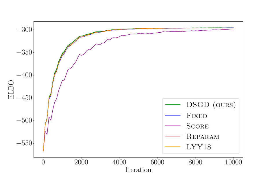
(a) textmsg

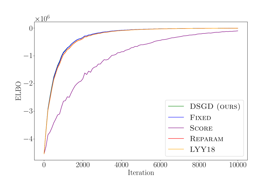
(b) influenza

Figure 3: ELBO trajectories for additional models. The same setup is used as in Fig. 2.

Table 4: Computational cost and work-normalised variances for additional models (cf. Table 2)

(a) textmsg

Estimator	Cost	$\textrm{Avg}(V(.))$	$V(\|.\|_{2})$
DSGD (ours)	1.84	7.89e-03	1.53e-02
Fixed	1.79	1.08e-02	2.14e-02
Reparam	1.25	7.99e-03	1.53e-02
LYY18	4.51	3.42e-02	6.00e-02

(b) influenza

Estimator	Cost	$\textrm{Avg}(V(.))$	$V(\|.\|_{2})$
DSGD (ours)	1.28	7.77e-03	3.94e-03
Fixed	1.28	7.92e-03	3.97e-03
Reparam	1.21	7.60e-03	3.75e-03
LYY18	8.30	5.80e-02	2.88e-02

Table 5: Mean of the final ELBO (the higher the better) for different random seeds and indicating error bars (the $\pm$ is one standard deviation).

(a) temperature

$\eta/\eta_{4000}$	DSGD (ours)	Fixed	Score	Reparam	LYY18
0.06	-76 $\pm$ 1	-624,250 $\pm$ 44,121
0.1	-84 $\pm$ 2	-425 $\pm$ 9
0.14	-15,476 $\pm$ 4,641	-121,932 $\pm$ 85,460	-2,611,479 $\pm$ 255,193	-706,729 $\pm$ 4,697	-17,502 $\pm$ 52,044
0.18	-94,125 $\pm$ 6,930	-32,171 $\pm$ 66
0.22	-165,787 $\pm$ 9,758	-155,321 $\pm$ 61,732

(b) xornet

$\eta/\eta_{4000}$	DSGD (ours)	Fixed	Score	Reparam
0.06	-3,530 $\pm$ 3,889	-5,522 $\pm$ 4,136
0.1	-33 $\pm$ 7	-2,029 $\pm$ 3,305
0.14	-27 $\pm$ 4	-2,028 $\pm$ 3,986	-553 $\pm$ 1,507	-9,984 $\pm$ 38
0.18	-25 $\pm$ 3	-26 $\pm$ 6
0.22	-30 $\pm$ 8	-26 $\pm$ 2

(c) random-walk

$\eta/\eta_{4000}$	DSGD (ours)	Fixed	Score	Reparam	LYY18
0.06	-37 $\pm$ 148	-85 $\pm$ 197
0.1	-37 $\pm$ 148	-86 $\pm$ 197
0.14	-38 $\pm$ 148	-37 $\pm$ 148	-85 $\pm$ 197	-371,612 $\pm$ 8,858	-135 $\pm$ 226
0.18	-38 $\pm$ 148	-37 $\pm$ 148
0.22	-38 $\pm$ 148	-37 $\pm$ 148

(d) cheating

$\eta/\eta_{4000}$	DSGD (ours)	Fixed	Score	Reparam	LYY18
0.06	-65 $\pm$ 1	-65 $\pm$ 1
0.1	-65 $\pm$ 1	-65 $\pm$ 1
0.14	-65 $\pm$ 1	-65 $\pm$ 1	-66 $\pm$ 1	-80 $\pm$ 1	-65 $\pm$ 1
0.18	-65 $\pm$ 1	-65 $\pm$ 1
0.22	-65 $\pm$ 1	-65 $\pm$ 1

(e) textmsg

$\eta/\eta_{4000}$	DSGD (ours)	Fixed	Score	Reparam	LYY18
0.06	-295 $\pm$ 1	-295 $\pm$ 1
0.1	-295 $\pm$ 1	-296 $\pm$ 1
0.14	-295 $\pm$ 1	-296 $\pm$ 1	-300 $\pm$ 1	-296 $\pm$ 1	-296 $\pm$ 1
0.18	-296 $\pm$ 1	-296 $\pm$ 1
0.22	-296 $\pm$ 1	-296 $\pm$ 1

(f) influenza

$\eta/\eta_{4000}$	DSGD (ours)	Fixed	Score	Reparam	LYY18
0.06	-3,586 $\pm$ 112	-3,589 $\pm$ 114
0.1	-3,584 $\pm$ 111	-3,590 $\pm$ 111
0.14	-3,582 $\pm$ 111	-3,590 $\pm$ 111	-95,380 $\pm$ 3,567	-4,045 $\pm$ 108	-3,860 $\pm$ 106
0.18	-3,579 $\pm$ 111	-3,589 $\pm$ 111
0.22	-3,577 $\pm$ 111	-3,587 $\pm$ 112

References

- Barthe et al., (2020) Barthe, G., Katoen, J.-P., and Silva, A., editors (2020). Foundations of Probabilistic Programming. Cambridge University Press.
- Bertsekas, (2015) Bertsekas, D. (2015). Convex optimization algorithms. Athena Scientific.
- Bertsekas and Tsitsiklis, (2000) Bertsekas, D. P. and Tsitsiklis, J. N. (2000). Gradient convergence in gradient methods with errors. SIAM J. Optim., 10(3):627–642.
- Bingham et al., (2019) Bingham, E., Chen, J. P., Jankowiak, M., Obermeyer, F., Pradhan, N., Karaletsos, T., Singh, R., Szerlip, P. A., Horsfall, P., and Goodman, N. D. (2019). Pyro: Deep universal probabilistic programming. J. Mach. Learn. Res., 20:28:1–28:6.
- Blake and Zisserman, (1987) Blake, A. and Zisserman, A. (1987). Visual Reconstruction. MIT Press.
- Blei et al., (2017) Blei, D. M., Kucukelbir, A., and McAuliffe, J. D. (2017). Variational inference: A review for statisticians. Journal of the American Statistical Association, 112(518):859–877.
- Botev and Ridder, (2017) Botev, Z. and Ridder, A. (2017). Variance Reduction. In Wiley StatsRef: Statistics Reference Online, pages 1–6.
- Davidson-Pilon, (2015) Davidson-Pilon, C. (2015). Bayesian Methods for Hackers: Probabilistic Programming and Bayesian Inference. Addison-Wesley Professional.
- Fu, (2006) Fu, M. C. (2006). Chapter 19 gradient estimation. In Henderson, S. G. and Nelson, B. L., editors, Simulation, volume 13 of Handbooks in Operations Research and Management Science, pages 575–616. North-Holland.
- Hazan et al., (2016) Hazan, E., Levy, K. Y., and Shalev-Shwartz, S. (2016). On graduated optimization for stochastic non-convex problems. In Balcan, M. and Weinberger, K. Q., editors, Proceedings of the 33nd International Conference on Machine Learning, ICML 2016, New York City, NY, USA, June 19-24, 2016, volume 48 of JMLR Workshop and Conference Proceedings, pages 1833–1841. JMLR.org.
- Hörmander, (2015) Hörmander, L. (2015). The Analysis of Linear Partial Differential Operators I: Distribution Theory and Fourier Analysis. Classics in Mathematics. Springer Berlin Heidelberg.
- Jang et al., (2017) Jang, E., Gu, S., and Poole, B. (2017). Categorical reparameterization with gumbel-softmax. In 5th International Conference on Learning Representations, ICLR 2017, Toulon, France, April 24-26, 2017, Conference Track Proceedings.
- Khajwal et al., (2023) Khajwal, B., Ong, C. L., and Wagner, D. (2023). Fast and correct gradient-based optimisation for probabilistic programming via smoothing. In Wies, T., editor, Programming Languages and Systems - 32nd European Symposium on Programming, ESOP 2023, Held as Part of the European Joint Conferences on Theory and Practice of Software, ETAPS 2023, Paris, France, April 22-27, 2023, Proceedings, volume 13990 of Lecture Notes in Computer Science, pages 479–506. Springer.
- Klenke, (2014) Klenke, A. (2014). Probability Theory: A Comprehensive Course. Universitext. Springer London.
- Lee et al., (2018) Lee, W., Yu, H., and Yang, H. (2018). Reparameterization gradient for non-differentiable models. In Advances in Neural Information Processing Systems 31: Annual Conference on Neural Information Processing Systems 2018, NeurIPS 2018, 3-8 December 2018, Montréal, Canada, pages 5558–5568.
- Maddison et al., (2017) Maddison, C. J., Mnih, A., and Teh, Y. W. (2017). The concrete distribution: A continuous relaxation of discrete random variables. In 5th International Conference on Learning Representations, ICLR 2017, Toulon, France, April 24-26, 2017, Conference Track Proceedings.
- Mak et al., (2021) Mak, C., Ong, C. L., Paquet, H., and Wagner, D. (2021). Densities of almost surely terminating probabilistic programs are differentiable almost everywhere. In Yoshida, N., editor, Programming Languages and Systems - 30th European Symposium on Programming, ESOP 2021, Held as Part of the European Joint Conferences on Theory and Practice of Software, ETAPS 2021, Luxembourg City, Luxembourg, March 27 - April 1, 2021, Proceedings, volume 12648 of Lecture Notes in Computer Science, pages 432–461. Springer.
- Minh and Gregor, (2014) Minh, A. and Gregor, K. (2014). Neural variational inference and learning in belief networks. In Proceedings of the 31th International Conference on Machine Learning, ICML 2014, Beijing, China, 21-26 June 2014, volume 32 of JMLR Workshop and Conference Proceedings, pages 1791–1799. JMLR.org.
- Mityagin, (2015) Mityagin, B. (2015). The zero set of a real analytic function.
- Mohamed et al., (2020) Mohamed, S., Rosca, M., Figurnov, M., and Mnih, A. (2020). Monte carlo gradient estimation in machine learning. J. Mach. Learn. Res., 21:132:1–132:62.
- Ranganath et al., (2014) Ranganath, R., Gerrish, S., and Blei, D. M. (2014). Black box variational inference. In Proceedings of the Seventeenth International Conference on Artificial Intelligence and Statistics, AISTATS 2014, Reykjavik, Iceland, April 22-25, 2014, pages 814–822.
- Reed and Simon, (2003) Reed, M. and Simon, B. (2003). Methods of Modern Mathematical Physics: Functional analysis. I. World Published Corporation.
- Rezende et al., (2014) Rezende, D. J., Mohamed, S., and Wierstra, D. (2014). Stochastic backpropagation and approximate inference in deep generative models. In Proceedings of the 31th International Conference on Machine Learning, ICML 2014, Beijing, China, 21-26 June 2014, volume 32 of JMLR Workshop and Conference Proceedings, pages 1278–1286. JMLR.org.
- Robbins and Monro, (1951) Robbins, H. and Monro, S. (1951). A stochastic approximation method. The annals of mathematical statistics, pages 400–407.
- Ruiz et al., (2016) Ruiz, F. J. R., Titsias, M. K., and Blei, D. M. (2016). The generalized reparameterization gradient. In Advances in Neural Information Processing Systems 29: Annual Conference on Neural Information Processing Systems 2016, December 5-10, 2016, Barcelona, Spain, pages 460–468.
- Schulman et al., (2015) Schulman, J., Heess, N., Weber, T., and Abbeel, P. (2015). Gradient estimation using stochastic computation graphs. In Cortes, C., Lawrence, N. D., Lee, D. D., Sugiyama, M., and Garnett, R., editors, Advances in Neural Information Processing Systems 28: Annual Conference on Neural Information Processing Systems 2015, December 7-12, 2015, Montreal, Quebec, Canada, pages 3528–3536.
- Shumway and Stoffer, (2005) Shumway, R. H. and Stoffer, D. S. (2005). Time Series Analysis and Its Applications. Springer Texts in Statistics. Springer-Verlag.
- Soudjani et al., (2017) Soudjani, S. E. Z., Majumdar, R., and Nagapetyan, T. (2017). Multilevel monte carlo method for statistical model checking of hybrid systems. In Bertrand, N. and Bortolussi, L., editors, Quantitative Evaluation of Systems - 14th International Conference, QEST 2017, Berlin, Germany, September 5-7, 2017, Proceedings, volume 10503 of Lecture Notes in Computer Science, pages 351–367. Springer.
- Sutton and Barto, (2018) Sutton, R. S. and Barto, A. G. (2018). Reinforcement Learning: An Introduction. The MIT Press, second edition.
- Tucker et al., (2017) Tucker, G., Mnih, A., Maddison, C. J., Lawson, D., and Sohl-Dickstein, J. (2017). REBAR: low-variance, unbiased gradient estimates for discrete latent variable models. In Guyon, I., von Luxburg, U., Bengio, S., Wallach, H. M., Fergus, R., Vishwanathan, S. V. N., and Garnett, R., editors, Advances in Neural Information Processing Systems 30: Annual Conference on Neural Information Processing Systems 2017, December 4-9, 2017, Long Beach, CA, USA, pages 2627–2636.
- van de Meent et al., (2018) van de Meent, J., Paige, B., Yang, H., and Wood, F. (2018). An introduction to probabilistic programming. CoRR, abs/1809.10756.
- Wingate and Weber, (2013) Wingate, D. and Weber, T. (2013). Automated variational inference in probabilistic programming. CoRR, abs/1301.1299.
- Xu et al., (2019) Xu, M., Quiroz, M., Kohn, R., and Sisson, S. A. (2019). Variance reduction properties of the reparameterization trick. In Chaudhuri, K. and Sugiyama, M., editors, The 22nd International Conference on Artificial Intelligence and Statistics, AISTATS 2019, 16-18 April 2019, Naha, Okinawa, Japan, volume 89 of Proceedings of Machine Learning Research, pages 2711–2720. PMLR.
- Zang, (1981) Zang, I. (1981). Discontinuous optimization by smoothing. Mathematics of Operations Research, 6(1):140–152.
- Zhang et al., (2019) Zhang, C., Bütepage, J., Kjellström, H., and Mandt, S. (2019). Advances in variational inference. IEEE Trans. Pattern Anal. Mach. Intell., 41(8):2008–2026.