In-Context Learning Demonstration Selection via Influence Analysis

Abstract

Large Language Models (LLMs) have demonstrated their In-Context Learning (ICL) capabilities which provides an opportunity to perform few shot learning without any gradient update. Despite its multiple benefits, ICL generalization performance is sensitive to the selected demonstrations. Selecting effective demonstrations for ICL is still an open research challenge. To address this challenge, we propose a demonstration selection method called InfICL which analyzes influences of training samples through influence functions. Identifying highly influential training samples can potentially aid in uplifting the ICL generalization performance. To limit the running cost of InfICL, we only employ the LLM to generate sample embeddings, and don’t perform any costly fine tuning. We perform empirical study on multiple real-world datasets and show merits of our InfICL against state-of-the-art baselines.

Keywords large language models $\cdot$ in-context learning $\cdot$ demonstration selection $\cdot$ influence functions

1 Introduction

Large Language Models (LLMs) have demonstrated their ability to perform few-shot inference through In-Context Learning (ICL) (Brown et al., 2020). Specifically, by providing a few demonstrations for the given task, the LLM is able to perform test case inference without performing any model gradient update.

ICL has several benefits such as few-shot learning, avoiding model fine-tuning, and versatility to different learning tasks. Despite these benefits, the ICL performance is sensitive to the selected demonstrations. To address this limitation, many different approaches have been proposed for demonstration selection, e.g., selecting demonstrations which are similar to the test case in the embedding space (Gao et al., 2021; Liu et al., 2022; Wu et al., 2023; Qin et al., 2023; Yang et al., 2022), learning a deep learning-based demonstration retriever (Rubin et al., 2022; Luo et al., 2023; Chen et al., 2020; Karpukhin et al., 2020; Scarlatos and Lan, 2023; Zhang et al., 2022; Li et al., 2023), selecting demonstrations based on LLM feedback (Li and Qiu, 2023; Chen et al., 2023; Wang et al., 2023), etc. However, there is lack of consensus regarding the most effective demonstration selection approach (Nguyen and Wong, 2023). The current research challenge is to identify those demonstrations which are the most effective or influential for improving the ICL generalization performance. We address this challenge by employing influence functions (Koh and Liang, 2017). Specifically, influence functions provide mechanisms to analyze effects or influences of training samples on the model without retraining the model. For example, influence functions can be used to analyze the model effects after up-weighting or removing a training sample. The training samples which have higher influences naturally provide more contributions to the model learning process. Intuitively, identifying these influential training samples can aid in improving the ICL generalization performance.

In this work, we focus on the text classification problem, and propose an influence function analysis-based demonstration selection method called InfICL. Since we need to perform influence function analysis on the training samples, an obvious approach is to calculate these influence scores by using the LLM itself (Grosse et al., 2023). However, for large and complex deep learning models, the influence function analysis becomes erroneous (Basu et al., 2021). Another approach is to fine tune the final layers of the LLM and perform influence function analysis by using these final layers. However, fine tuning LLM is a highly resource intensive task. To address these practical challenges, we only employ the LLM to generate sample embeddings. By employing these LLM generated training sample embeddings, we train a simple classifier. We analyze the influence of each training sample by using the classifier and a validation set. Finally, we select the most influential training samples from each class as the demonstration set. We summarize our main contributions below.

• We propose a ICL demonstration selection method called InfICL which is based on influence function analysis.

• We present a theoretical analysis study to show that under certain scenarios, the influential samples for the classifier are also the influential samples for the LLM. Thereby, we connect the influence analysis done by using the classifier with the LLM.

• We present an empirical study conducted on multiple real-world datasets. In this empirical study, we show that our InfICL can outperform the contemporary demonstration selection methods.

2 Related Work

Our work mainly focuses on designing an demonstration selection method for ICL through influence analysis.

Demonstration Selection. Recently, the problem of demonstration selection for ICL has received a significant attention in the literature. We direct the interested readers to (Liu et al., 2021; Dong et al., 2023) for detailed surveys regrading different demonstration selection methods. One of the popular approaches for demonstration selection is to select those training points as demonstrations which are similar to the test sample in the embedding space (Gao et al., 2021; Liu et al., 2022; Wu et al., 2023; Qin et al., 2023; Yang et al., 2022).

Another popular approach is to employ a demonstration retriever to perform demonstration selection. Specifically, the demonstration retriever is a deep learning based model. Rubin et al. (2022) and Luo et al. (2023) train their demonstration retriever by employing contrastive loss (Chen et al., 2020). Li et al. (2023) employ in-batch negative loss (Karpukhin et al., 2020). Scarlatos and Lan (2023) and Zhang et al. (2022) employ reinforcement learning to train their demonstration retriever. In our work, we do not utilize any complex demonstration retriever, and design a simple method which operates on LLM embeddings.

Recently, LLM feedback based demonstration selection methods have been proposed. Specifically, the LLM is queried for its prediction confidence on each training point. Li and Qiu (2023) identify training points which are more informative. Chen et al. (2023) select training points which are less sensitive to predictions. Wang et al. (2023) fine tune the LLM by using only the final emdedding layer and model the demonstration selection as a topic model. These methods can also be considered as influence based methods because they analyze the influence of training points by using direct LLM feedback.

Influence Functions. For machine learning applications, influence functions have been used for different tasks, e.g., filtering or relabeling mislabeled training data (Kong et al., 2022), designing data poisoning attacks (Fang et al., 2020; Jagielski et al., 2021), designing data augmentation strategies (Lee et al., 2020; Oh et al., 2021), and analyzing label memorization effects (Feldman and Zhang, 2020). For LLMs, influence functions have been used to identify data artifacts (Han et al., 2020), identify biases in word embeddings (Brunet et al., 2019), and explaining the LLM performance (Grosse et al., 2023; Han and Tsvetkov, 2021).

Influence analysis can be broadly divided into two categories: retraining based (Ilyas et al., 2022) and gradient based methods also called as influence functions (Koh and Liang, 2017). The retraining based methods collect random subsets of the training set. Then, the influence of each training point in the collected subset is calculated by either model retraining or by learning a linear surrogate. However, the retraining based methods have high running costs, and are not scalable to large datasets because to effectively cover all the training points, a large number of subsets have to be constructed and evaluated (Grosse et al., 2023).  Nguyen and Wong (2023) and Chang and Jia (2023) employ retraining based influence analysis to construct the demonstration sets and as a result, their proposed demonstration selection methods incur high running costs. We provide a detailed design description about these demonstration selection methods and compare their running costs against our InfICL in Section 3.2. Specifically, we show that by using the gradient based influence analysis for constructing demonstration sets, we can overcome the high running cost challenge associated with the retraining based influence analysis methods.

3 Proposed Method

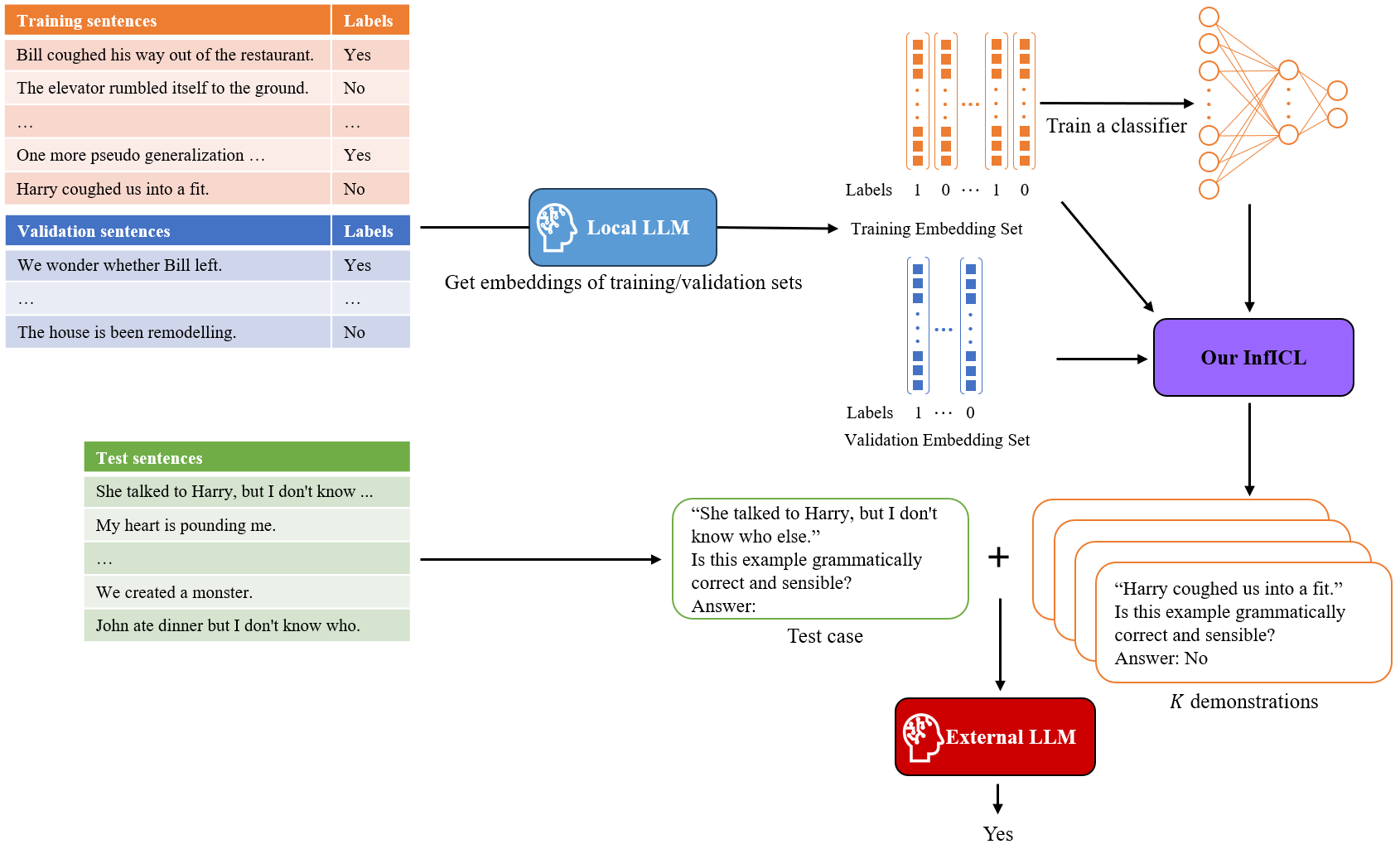
Figure 1: Illustration of ICL for the text classification task through our InfICL. Initially, by employing the local LLM, embeddings for all the training and validation set inputs are generated. A local classifier is then trained by employing training input embeddings and labels. InfICL determines $K$ demonstration examples based on influence scores. Finally, the demonstration set and each test case are sent to an external LLM for inference.

We consider the task classification task having a training set $\mathcal{T}$ with $n$ training points denoted as $z_{i}=\{(\mathbf{x}_{i},y_{i})\}_{i=1}^{n}$. Here, $\mathbf{x}_{i}$ and $y_{i}$ denote the embedding vector for the $i^{th}$ training sample input $s_{i}$ and its corresponding label, respectively. Let $\mathcal{C}$ denote the class set for the target variable $y_{i}$ and $y_{i}\in\mathcal{C}$. We employ a validation set $\mathcal{V}$.

3.1 Algorithm

Figure 1 shows our influence based demonstration selection framework. We employ separate LLMs for demonstration selection and test case inference called local LLM $\mathcal{P}$ and external LLM $\mathcal{Q}$, respectively. For internal LLM $\mathcal{P}$, to reduce training costs, we employ a light-weight LLM and use it to generate embeddings for the input texts wherein, $\mathbf{x}_{i}=\mathcal{P}(s_{i})$. For external LLM $\mathcal{Q}$, we opt a powerful and heavier LLM. We include a local classifier denoted as $\mathcal{F}(\mathbf{x}_{i},\theta)$ with the input of embeddings and parameterized with $\theta$. We denote $\mathcal{L}_{f}(z_{i},\theta)$ as the classifier training loss.

Our goal is to select $K$ suitable demonstrations for the given text classification task. Note that $K$ is analogous to the number of shots in few-shot learning and is constrained by the employed external LLM. We employ a balanced selection approach wherein we select equal number of demonstrations from each class $c\in\mathcal{C}$. Specifically, we select $R$ ($R=\left\lfloor K/|\mathcal{C}|\right\rfloor$) suitable training set points from each class as demonstrations.

Algorithm 1 InfICL demonstration selection.

1:Inputs: $\mathcal{T}$, $\mathcal{V}$, $\mathcal{F}$, $\mathcal{L}_{f}$, $R$, and $\mathcal{P}$.

2:Output: demonstration set $\cup_{c\in\mathcal{C}}\{z_{i}^{c}\}_{i=1}^{R}$.

3:generate embeddings for all training and validation inputs through $\mathcal{P}$;

4:for each training epoch do

5:     train classifier $\mathcal{F}$ on $\mathcal{T}$ by using $\mathcal{L}_{f}$;

6:for each $z_{i}=\left(\mathbf{x}_{i},y_{i}\right)\in\mathcal{T}$ do

7:     calculate its influence score by using Eq 2;

8:for each class $c\in\mathcal{C}$ do

9:     select top-$R$ training points $\{z_{i}^{c}\}_{i=1}^{R}$ from $\mathcal{T}$ based on influence scores;

10:return $\cup_{c\in\mathcal{C}}\{z_{i}^{c}\}_{i=1}^{R}$

Algorithm 1 shows the pseudo code of our InfICL. The inputs include training set $\mathcal{T}$, validation set $\mathcal{V}$, classifier $\mathcal{F}$, loss $\mathcal{L}_{f}$, the number of demonstration examples per class $R$, and local LLM $\mathcal{P}$. Initially, by employing the local LLM $\mathcal{P}$, we generate embeddings for all training and validation inputs. In lines 2-4, we train the local classifer $\mathcal{F}$ using the embeddings and labels. Next, we calculate influence score of each training point (lines 5-7). For each class $c\in\mathcal{C}$, we select the top-$R$ training points $\{z_{i}^{c}\}_{i=1}^{R}$ as demonstrations from $\mathcal{T}$ based on influence scores (lines 8-10). Finally, we return the constructed demonstration set $\cup_{c\in\mathcal{C}}\{z_{i}^{c}\}_{i=1}^{R}$.

Influence Functions. The main goal of the influence functions is to study the effect of training points on model prediction (Koh and Liang, 2017). Influence functions provide a practical solution wherein the model parameter change can be studied without retraining the model. Let $\frac{1}{n}\sum_{i=1}^{n}\mathcal{L}_{f}(z_{i},\theta)$ be the empirical risk and its minimizer is given by $\widehat{\theta}=\arg\min_{\theta\in\Theta}\frac{1}{n}\sum_{i=1}^{n}\mathcal{L}_{f}(z_{i},\theta)$. It is assumed that the empirical risk is twice differentiable and strictly convex. However, this assumption can be practically relaxed. The influence of up-weighting training point $z$ on the classifier parameter $\theta$ can be calculated by using the influence function as

$$\mathcal{I}_{\textit{up,params}}(z)=\derivative{\widehat{\theta}_{\epsilon,z}}{\epsilon}\Bigg{|}_{\epsilon=0}=-H^{-1}_{\widehat{\theta}}\gradient_{\theta}\mathcal{L}_{f}(z,\widehat{\theta}),$$ (1)

where $H_{\widehat{\theta}}=\frac{1}{n}\sum_{i=1}^{n}\gradient_{\theta}^{2}\mathcal{L}_{f}(z_{i},\widehat{\theta})$ is the Hessian and it is positive definite by assumption. Next, the influence of up-weighting $z$ on the loss $\mathcal{L}_{f}$ at a validation point $z_{val}\in\mathcal{V}$ is given by

$$\mathcal{I}_{\textit{up,loss}}(z,z_{val})=-\gradient_{\theta}{\mathcal{L}_{f}(z_{val},\widehat{\theta})}^{\top}H^{-1}_{\widehat{\theta}}\gradient_{\theta}\mathcal{L}_{f}(z,\widehat{\theta}).$$

For the entire validation set $\mathcal{V}$, the influence of up-weighting $z$ on the loss $\mathcal{L}_{f}$ at $\mathcal{V}$ is given by

$$\mathcal{I}_{up,loss}(z,\mathcal{V})=-\left[\dfrac{1}{|\mathcal{V}|}\sum_{z_{j}\in\mathcal{V}}\gradient_{\theta}\mathcal{L}_{f}\left(z_{j},\widehat{\theta}\right)\right]^{\top}H_{\widehat{\theta}}^{-1}\gradient_{\theta}\mathcal{L}_{f}\left(z,\widehat{\theta}\right)$$ (2)

Specifically, the highly influential training points are those with most positive ($-\mathcal{I}_{\textit{up,loss}}(z,\mathcal{V})$) scores (Koh and Liang, 2017). We employ $Inf(z,\mathcal{V})=-\mathcal{I}_{\textit{up,loss}}(z,\mathcal{V})$ as the influence score to analyze the influence of up-weighting each training point $z$ on the loss $\mathcal{L}_{f}$ at $\mathcal{V}$. This is because, the training points which have high influences on the validation loss provide richer information for model learning, and can become better demonstrations for the ICL task.

Personalized Demonstration Selection. We can easily extend InfICL to construct a personalized demonstration set for each test case $x_{test}$. Specifically, we can extend InfICL to this setting by scoring each training point $z_{i}\in\mathcal{T}$ as

$$score(z_{i})=\lambda Inf(z_{i},\mathcal{V})+(1-\lambda)sim(\mathbf{x}_{i},\mathbf{x}_{test})$$ (3)

where $sim(\cdot,\cdot)$ denotes the cosine similarity between the input embeddings, and $\lambda$ is the weight which can be set by analyzing the accuracy performance on the validation set. The top-$R$ training points from each class based on $score(z_{i})$ are included in the demonstration set.

3.2 Running Cost Analysis

In this section, we study the running costs of our InfICL along with other influence analysis based demonstration selection methods, Influence (Nguyen and Wong, 2023) and Curation (Chang and Jia, 2023). Note that both methods employ retraining based influence analysis approach and our InfICL employs gradient based influence analysis approach. We show running cost benefits of our InfICL over Influence and Curation.

We quantify the running costs of demonstration selection methods by analyzing the total number of LLM access (API) calls for both local and external LLMs. Specifically, the unit cost of local LLM ($\mathcal{P}$) access call for generating an embedding for a single training point is denoted as $C_{\mathcal{P}}$. Similarly, the unit cost of external LLM ($\mathcal{Q}$) access call for performing inference on a single test or validation case is denoted as $C_{\mathcal{Q}}$. Note that $C_{\mathcal{Q}}$ is usually much higher than $C_{\mathcal{P}}$. This is because $C_{\mathcal{Q}}$ involves ICL cost w.r.t external LLM and $C_{\mathcal{P}}$ only generates the final layer embeddings which only incurs model forward pass cost. We show the running costs of different influence analysis based demonstration selection methods in Table 1 and provide a detailed description below.

Table 1: Running cost analysis of influence analysis based demonstration selection methods.

Methods	Influence (Nguyen and Wong, 2023)	Curation (Chang and Jia, 2023)		InfICL
		CondAcc	Data Models
Running Cost	$\mathcal{O}\left(C_{\mathcal{Q}}|\mathcal{V}|M\right)$	$\mathcal{O}\left(C_{\mathcal{Q}}|\mathcal{V}|MK!\right)$	$\mathcal{O}\left(C_{\mathcal{Q}}|\mathcal{V}|M\right)$	$\mathcal{O}\left(C_{\mathcal{P}}|\mathcal{T}|+C_{\mathcal{Q}}\right)$

InfICL. We generate embeddings for all training points and generating embedding for each training point requires a single local LLM access call. Thus, the total cost of local LLM access calls for embedding generation is $C_{\mathcal{P}}|\mathcal{T}|$. For the test case inference, we require a single external LLM access call and the cost is $C_{\mathcal{Q}}$. Thus, the the running cost of our demonstration selection method is given by $\mathcal{O}\left(C_{\mathcal{P}}|\mathcal{T}|+C_{\mathcal{Q}}\right)$. For influence estimation, we use a fully connected neural network as the backbone architecture for the classifier $\mathcal{F}$. Let $d$ is the number of parameters in $\mathcal{F}$. Calculating the loss of $|\mathcal{T}|$ training samples takes $\mathcal{O}(d|\mathcal{T}|)$. In the implementation, we use LiSSA (Agarwal et al., 2017) method to approximate the inverse Hessian-Vector product (iHVP) of $\left[\dfrac{1}{|\mathcal{V}|}\sum_{z_{j}\in\mathcal{V}}\gradient_{\theta}\mathcal{L}_{f}\left(z_{j},\widehat{\theta}\right)\right]^{\top}H_{\widehat{\theta}}^{-1}$, which requires $\mathcal{O}(|\mathcal{V}|d+rjd)$ where $r$ is the recursion depth and $j$ is the number of repeats. As both validation set and $\theta$ are fixed, there is only one computation of iHVP. The sorting time needed for ranking potential demonstrations by influence is $\mathcal{O}(|\mathcal{T}|\log(|\mathcal{T})|$ on average. Consequently, the influence estimation process takes $\mathcal{O}(d|\mathcal{T}|+|\mathcal{V}|d+rjd+|\mathcal{T}|\log(|\mathcal{T})|$. In a practical setting, $|\mathcal{V}|$ is sufficiently small compared to $\mathcal{|T|}$ ($|\mathcal{V}|\ll\mathcal{|T|}$) and $rj\approx|\mathcal{T}|$. Therefore, the running time for calculating influence scores is $\mathcal{O}(d|\mathcal{T}|+|\mathcal{T}|\log(|\mathcal{T})|$.

Influence (Nguyen and Wong, 2023). Initially, $M$ random demonstrations are constructed from $\mathcal{T}$. For each constructed demonstration set $S_{i}$ where $|S_{i}|=K$, its ICL generalization performance on the entire validation set $\mathcal{V}$ is calculated by using the external LLM. Then, the influence of each training point $z_{j}\in S_{i}$ is calculated as the difference between the average performance of demonstration sets including $z_{j}$ and the average performance of demonstration sets omitting $z_{j}$. Through this design analysis, we can infer the running cost of Influence as $\mathcal{O}\left(C_{\mathcal{Q}}|\mathcal{V}|M\right)$.

Curation (Chang and Jia, 2023). There are two variants: CondAcc and Data Models. Specifically, the CondAcc variant is almost similar to Influence. However, for each constructed random demonstration set, the ICL generalization performance of its each permutation on $\mathcal{V}$ is separately evaluated. Thereby, the running cost of CondAcc is given by $\mathcal{O}\left(C_{\mathcal{Q}}|\mathcal{V}|MK!\right)$. In the Data Models variant, a surrogate linear model is trained to mimic the prediction performance of the external LLM. Similar to Influence, $M$ random demonstration sets are constructed. Each random demonstration set is used to train a separate linear model. For a given random demonstration set, the employed linear model training loss calculates the difference between generalization performances of linear model and external LLM (based on ICL) on the validation set. After this training, the influence of each training point belonging to a random demonstration set is calculated by analyzing the linear model parameters. Through this design analysis, we can infer the running cost of Data Models as $\mathcal{O}\left(C_{\mathcal{Q}}|\mathcal{V}|M\right)$.

The running costs of both Influence and Curation are dominated by the term $C_{\mathcal{Q}}|\mathcal{V}|M$. Here, $M$ which denotes the number of constructed random demonstration sets needs to be large in-order to effectively cover the entire training set, and to obtain good estimates of influence scores (Nguyen and Wong, 2023). As a consequence, both Influence and Curation incur an extremely large amount of external LLM access calls. For InfICL, we approximately require $|\mathcal{T}|$ local LLM access calls, which makes InfICL much more cost-effective than both Influence and Curation.

3.3 Theoretical Analysis

For the training point $z_{i}=(\mathbf{x}_{i},y_{i})$, we calculate the next token prediction loss by employing only the input $s_{i}$ where $\mathbf{x}_{i}=\mathcal{P}(s_{i})$. Let $\mathcal{L}_{nt}$ denote the next token prediction loss. For our theoretical analysis, to differentiate the influence functions for the classifier $\mathcal{F}$ and local LLM $\mathcal{P}$, we employ the following notations: for $\mathcal{F}$, we employ the notation $\mathcal{I}_{\textit{up,params}}(z_{i},\theta)$ for $\theta\in\Theta$; for local LLM $\mathcal{P}$, we denote up-weighted influence for $\mathcal{P}$ as $\mathcal{I}_{\textit{up,params}}(s_{i},\phi)$ where $\phi\in\Phi$ and $\Phi$ denotes the local LLM ($\mathcal{P}$) parameter space. Here, the up-weighted influence for local LLM $\mathcal{P}$ is given by:

$$\mathcal{I}_{\textit{up,params}}(s_{i},\phi)=\derivative{\widehat{\phi}_{\epsilon,s_{i}}}{\epsilon}\Bigg{|}_{\epsilon=0}=-H^{-1}_{\widehat{\phi}}\gradient_{\phi}\mathcal{L}_{nt}(s_{i},\widehat{\phi})$$ (4)

Theorem 1.

Suppose the embedding space is clustered wherein the training points in the same cluster share the same label. For the two training points $z_{i}=(\mathbf{x}_{i},y_{i})$ and $z_{j}=(\mathbf{x}_{j},y_{j})$,

$$\begin{split}&\mathcal{I}_{\textit{up,params}}(s_{i},\phi)\leq\mathcal{I}_{\textit{up,params}}(s_{j},\phi)\\ &\iff\mathcal{I}_{\textit{up,params}}(z_{i},\theta)\leq\mathcal{I}_{\textit{up,params}}(z_{j},\theta)\end{split}$$

Theorem 1 states that if the embedding space is clustered with training points belonging to the same cluster share the same label then, if a training input has high influence for $\mathcal{P}$, it will also have high influence for $\mathcal{F}$. We provide the proof in Appendix A. The requirement that the embedding space is clustered is not unrealistic because $\mathcal{P}$ tends to generate closer embeddings for those training inputs which are similar to each other and sharing the same label. From Theorem 1, we can infer that the influential training points for $\mathcal{F}$ can be employed as an effective ICL demonstrations.

4 Experiments

4.1 Experimental Setup

Datasets. We use two real-world datasets for our empirical evaluation study, Corpus of Linguistic Acceptability (CoLA) (Warstadt et al., 2018) and Recognizing Textual Entailment (RTE) (Dagan et al., 2005). The CoLA dataset contains sentences from different linguistics publications, which are expertly annotated for grammatical acceptability by their original authors. Each sentence is either labeled as acceptable or unacceptable. The RTE dataset sample contains two text fragments denoted as premise and hypothesis, and the corresponding label indicates whether the meaning of the hypothesis can be inferred from the text (yes or no). Table 2 shows the dataset details including training, validation and test set split.

Table 2: Dataset Details.

Dataset	Size	+ve Class	$\bm{|\mathcal{T}|}$	$\bm{|\mathcal{V}|}$	Test Set Size
CoLA	9594	70%	8466	85	1043
RTE	2717	50%	2466	24	277

Baselines. For our empirical study, we employ five baselines: (1) Classifier: we directly employ a single layer neural network; (2) Zero-shot: this baseline directly performs test case inference without any demonstrations; (3) Random: demonstrations are selected based on random sampling; (4) RICES (Yang et al., 2022): the training points are scored based on their cosine similarity to the test sample in the embedding space and then the top-$R$ training points from each class are selected as demonstrations; (5) Influence (Nguyen and Wong, 2023): it is one of state-of-the-art influence analysis based demonstration selection methods which we have described in Section 3.2.

Training Details. We employ Llama-2-7B (Touvron et al., 2023) as the local LLM. For the external LLM, we separately evaluate on Llama-2-7B, Llama-2-13B, and OPT-6.7B. The embedding size is 4096. For the classifier, we employ a fully connected neural network with three layers. All experiments are executed on GPU Tesla V100 (32GB RAM) and CPU Xeon 6258R 2.7 GHz. We use the Adam optimizer with learning rates {0.001, 0.01} and 20 training epochs.

4.2 Experimental Results

Table 3: Performances of our InfICL and non-influence analysis based baselines (mean±std) for external LLMs. Scores are reported after 5 runs. Higher the better for accuracy and F1 scores. For each external LLM, the best values for each shot are bold highlighted. ‘N/A’ denotes non-applicable and ‘–’ denotes non-feasible results due to the limitation of LLM’s context length.

External LLM ($\mathcal{Q}$)	Shots ($K$)	Method	CoLA		RTE
			Accuracy (%)	F1	Accuracy (%)	F1
N/A	N/A	Classifier	82.83 ±0.00	88.18 ±0.00	57.76 ±0.00	58.95 ±0.00
LLama-2-7B	0	Zero-shot	63.39 ±0.00	68.81 ±0.00	69.19 ±0.00	68.83 ±0.00
	8	Random	70.35 ±3.68	75.70 ±4.53	74.97 ±0.21	77.31 ±1.19
		RICES	70.74 ±0.41	78.50 ±0.28	77.38 ±1.16	80.34 ±0.61
		InfICL	70.89 ±0.77	77.23 ±1.18	77.26 ±1.25	80.16 ±1.36
	16	Random	70.20 ±2.30	75.54 ±2.6	77.02 ±0.83	79.24 ±1.20
		RICES	73.71 ±0.52	80.97 ±0.42	76.77 ±1.37	80.44 ±1.29
		InfICL	74.75 ±1.32	81.39 ±0.92	78.58 ±0.55	80.98 ±0.41
	32	Random	73.00 ±1.68	78.74 ±2.00	77.38 ±1.10	79.87 ±1.02
		RICES	74.02 ±0.51	80.96 ±0.86	73.89 ±0.55	75.86 ±0.48
		InfICL	73.48 ±0.74	79.50 ±1.19	77.74 ±0.55	79.92 ±1.14
LLama-2-13B	0	Zero-shot	50.07 ±0.00	45.29 ±0.00	77.25 ±0.00	78.82 ±0.00
	8	Random	73.17 ±3.76	78.53 ±5.15	80.39 ±0.21	82.51 ±0.80
		RICES	73.42 ±0.92	81.37 ±0.75	77.86 ±1.16	81.89 ±0.84
		InfICL	76.66 ±1.71	82.31 ±1.47	82.43 ±2.21	84.25 ±1.74
	16	Random	75.40 ±1.48	81.48 ±1.98	82.31 ±1.57	84.08 ±1.29
		RICES	73.94 ±0.88	82.11 ±0.48	79.66 ±1.37	82.80 ±1.27
		InfICL	77.47 ±0.32	84.58 ±0.47	83.63 ±0.21	85.08 ±0.39
	32	Random	75.95 ±1.74	83.06 ±1.27	81.76 ±1.26	82.49 ±1.54
		RICES	73.23 ±0.70	82.12 ±0.69	77.08 ±0.91	77.70 ±0.99
		InfICL	76.05 ±0.81	84.20 ±0.41	82.67 ±1.08	83.67 ±1.14
OPT-6.7B	0	Zero-shot	66.92 ±0.00	80.07 ±0.00	54.15 ±0.00	60.44 ±0.00
	8	Random	63.37 ±0.17	75.43 ±2.64	56.92 ±2.73	67.98 ±2.81
		RICES	64.30 ±0.11	76.85 ±0.20	55.60 ±1.30	69.02 ±0.06
		InfICL	63.50 ±0.78	76.76 ±0.33	57.76 ±0.63	70.43 ±0.80
	16	Random	62.03 ±0.50	77.07 ±2.87	54.51 ±0.63	63.84 ±0.86
		RICES	63.69 ±0.06	76.03 ±0.01	52.11 ±1.10	66.31 ±0.68
		InfICL	63.79 ±0.55	76.48 ±0.70	57.28 ±0.91	70.14 ±0.50
	32	Random	59.66 ±0.70	72.24 ±1.62	–	–
		RICES	61.39 ±0.22	74.38 ±0.32	–	–
		InfICL	61.77 ±0.77	73.48 ±1.60	–	–

Table 4: Student’s t-test analysis results for demonstration selection methods based on accuracy scores. The p-value is calculated by using the accuracy scores for all shots and runs.

External LLM	Dataset	Method 1	Method 2	p-value
LLama-2-7B	CoLA	InfICL	Random	0.0449
			RICES	0.7363
	RTE	InfICL	Random	0.0207
			RICES	0.0286
LLama-2-13B	CoLA	InfICL	Random	0.0229
			RICES	0.0007
	RTE	InfICL	Random	0.0384
			RICES	0.0005
OPT-6.7B	CoLA	InfICL	Random	0.0686
			RICES	0.8550
	RTE	InfICL	Random	0.1190
			RICES	0.0075

Comparison to non-influence analysis based baselines. We show performances of our InfICL and non-influence analysis based baselines on external LLMs in Table 3. We also perform student’s t-test analysis. We perform this analysis on accuracy scores. Specifically, we consider the accuracy scores for all shots and runs to calculate the p-value. We show the result in Table 4. Zero-shot does not involve any demonstrations. Therefore, the external LLM does not get any opportunity to better understand the given task and as a result, Zero-shot performance is not noticeable.

For LLama-2-7B and for the RTE dataset, InfICL outperforms Random w.r.t all shots. The corresponding p-value (refer to Table 4) between InfICL and Random is 0.0207 which indicates that InfICL performs statistically significant better than Random. InfICl also outperforms RICES for 16 and 32 shots. Even though RICES outperforms InfICL for 8 shots, we show that the overall performance of InfICL across all shots and runs is statistically significant and better than RICES. The mean accuracy performance of InfICL and RICES across all runs and shots is 77.85% and 76.67%, respectively. The corresponding p-value is 0.0286 which indicates that InfICL has an overall statistically significant better performance than RICES. For the CoLA dataset, InfICL again outperforms Random w.r.t all shots and with a statistically significant result. InfICL outperforms RICES for 8 and 16 shots. However, RICES outperforms InfICL for 32 shots. This is because, in rare cases, selecting personalized demonstrations can aid in improving the performance when compared to analyzing the training point influences.

For LLama-2-13B and for both datasets, InfICL achieves statistically significant better results than both Random and RICES w.r.t all shots. Random under-performs against InfICL, showing randomly selecting training points as demonstrations generally does not provide satisfactory results. Even though RICES provides personalized demonstrations for each test case by identifying similar training inputs to the test case in the embedding space, it does not select highly influential demonstrations, which is crucial to aid the ICL performance. As a consequence it under-performs against InfICL.

For OPT-6.7B and for the CoLA dataset, p-values for Random and RICES when compared against InfICL are 0.0686 and 0.8550, respectively. This shows that the performance results for this dataset are not statistically significant. For the RTE dataset, InfICL achieves statistically significant and better result than RICES based on the p-value which is 0.0075.

Table 5: Test accuracy of our InfICL and Influence on different external LLMs. Asterik denotes the results extracted from (Nguyen and Wong, 2023).

External LLM	Dataset	Shots	InfICL	Influence
OPT-6.7B	CoLA	16	66.40	46.80
		32	68.20	58.60
	RTE	12	51.20	$62.70^{*}$
LLama-2-7B	CoLA	16	75.55	73.20
		32	72.00	74.40
	RTE	12	78.80	$65.70^{*}$

Comparison to influence analysis based baseline. We compare our InfICL to Influence (Nguyen and Wong, 2023). Since Influence has an extremely high running costs, it can only run on a small size training and validation sets. To conduct a fair comparison, we run our InfICL in the same dataset setting as mentioned in (Nguyen and Wong, 2023), which has train/validation/test size as 400/200/500, respectively. We show the empirical results in Table 5. For LLama2-7B, InfICL overall significantly outperforms Influence w.r.t all shots on both CoLA and RTE datasets. However, for OPT-6.7B, although InfICL significantly outperforms Influence w.r.t both 16 and 32 shots on the CoLA dataset, InfICL has a lower accuracy (51.2%) than Influence (62.70%) on the RTE dataset. This indicates the chosen 12 demonstraton examples based on InfICL do not convey sufficient information that can be exploited by OPT-6.7B. In our future work, we will study whether our personalized InfICL, which generate different demonstration examples for each test example, can produce better performance. For the setting of Llama-2-7B and 32 shots on CoLA dataset, our InfICL takes 10 minutes and Influence takes 8 hours.

5 Conclusion

In this work, we have proposed a demonstration selection method for ICL based on analyzing influences of training samples through influence functions. Our method employs a local LLM to generate sample embeddings and avoids costly fine tuning of the LLM. We presented a theoretical analysis study to connect the influential analysis between the LLM and the inference classifier which employs the LLM embeddings as inputs. The empirical study on multiple real-world datasets showed merits of our method against state-of-the-art baselines. In our future work, we will conduct evaluations with more LLMs and datasets.

Even though we have shown that influence function analysis can be useful to select ICL demonstrations, we have not provided a strong interpretability study on why influence functions aid in improving ICL performance. We have used influence functions based on the intuition that highly influential training samples are useful for model learning. However, ICL does not perform any model gradient update, and it is considerably different from gradient update-based learning. We need to connect mechanisms of ICL with gradient update-based models through a theoretical study (Xie et al., 2022) and show that highly influential training samples can also aid in improving the ICL performance. We also plan to extend our demonstration selection method to large vision models (LVMs).

Appendix A Proof for Theorem 1

We divide the clusters in the embedding space as dense and sparse clusters. Specifically, dense and sparse clusters have large and limited cluster cardinalities, respectively. We will first establish the scenario where the condition $\mathcal{I}_{\textit{up,params}}(s_{i},\phi)\leq\mathcal{I}_{\textit{up,params}}(s_{j},\phi)$ can be satisfied for the local LLM. For our proof sketch, we will consider the stochastic gradient descent optimization algorithm. For a training input $s_{i}$, during the $k^{th}$ training iteration, we have that $\widehat{\phi}_{k+1}=\widehat{\phi}_{k}-\partialderivative{\mathcal{L}_{nt}(s_{i})}{\phi}$. Here, $\widehat{\phi}_{k}$ denotes the estimated parameter for $\phi$ after the $k-1$ training iteration. Now we will perform a training intervention action wherein, in the next iteration, instead of selecting a random training input, we will again select $s_{i}$. We have that $\widehat{\phi}_{k+2}=\widehat{\phi}_{k+1}-\partialderivative{\mathcal{L}_{nt}(s_{i})}{\phi}$. Since the gradient descent algorithm results in the convergence of the parameter $\phi$, for this intervention action, we can infer that $|\widehat{\phi}_{k+2}-\widehat{\phi}_{k+1}|\leq|\widehat{\phi}_{k+1}-\widehat{\phi}_{k}|$. Now consider a practical scenario wherein, we select a training input $s_{r}$ from the same cluster to which $s_{i}$ belongs in the embedding space. We have that $\widehat{\phi}_{k+2}=\widehat{\phi}_{k+1}-\partialderivative{\mathcal{L}_{nt}(s_{r})}{\phi}$. Since the training inputs from the same cluster can share significant similarities and also have the same label, optimizing with $s_{r}$ can produce similar consequence which resulted by optimizing through the intervention action. Hence, we can hypothesize that $|\widehat{\phi}_{k+2}-\widehat{\phi}_{k+1}|\leq|\widehat{\phi}_{k+1}-\widehat{\phi}_{k}|$.

From this analysis, we can infer that even though due to high caridnality, a dense cluster involves significantly in the parameter estimation process, the individual training points belonging to this dense cluster can be hypothesized to have limited influences. For example, if $s_{i}$ belongs to a dense cluster then, its influence is low because even if $s_{i}$ is removed from the training process, there will be numerous other training inputs such as $s_{r}$ which are closely similar to $s_{i}$ and share the same label, which will effectively cover the absence of $s_{i}$ in the training process. If $s_{i}$ belongs to a sparse cluster then, there are only few training inputs in the cluster which can effectively cover $s_{i}$ in the training process. Hence, the training inputs belonging to a sparse cluster can be hypothesized to have higher influences. Hence, if $s_{i}$ and $s_{j}$ belong to dense and sparse clusters in the embedding space, respectively we have that $\mathcal{I}_{\textit{up,params}}(s_{i},\phi)\leq\mathcal{I}_{\textit{up,params}}(s_{j},\phi)$.

Note that our classifier inputs come from the same embedding space generated by the local LLM. Hence, we can apply the same analysis outlined above for our classifier and get the result $\mathcal{I}_{\textit{up,params}}(z_{i},\theta)\leq\mathcal{I}_{\textit{up,params}}(z_{j},\theta)$.

References

- Brown et al. [2020] Tom Brown, Benjamin Mann, Nick Ryder, Melanie Subbiah, Jared D Kaplan, Prafulla Dhariwal, Arvind Neelakantan, Pranav Shyam, Girish Sastry, Amanda Askell, Sandhini Agarwal, Ariel Herbert-Voss, Gretchen Krueger, Tom Henighan, Rewon Child, Aditya Ramesh, Daniel Ziegler, Jeffrey Wu, Clemens Winter, Chris Hesse, Mark Chen, Eric Sigler, Mateusz Litwin, Scott Gray, Benjamin Chess, Jack Clark, Christopher Berner, Sam McCandlish, Alec Radford, Ilya Sutskever, and Dario Amodei. Language models are few-shot learners. In Advances in Neural Information Processing Systems, 2020.
- Gao et al. [2021] Tianyu Gao, Adam Fisch, and Danqi Chen. Making pre-trained language models better few-shot learners. In Proceedings of the 59th Annual Meeting of the Association for Computational Linguistics and the 11th International Joint Conference on Natural Language Processing, 2021.
- Liu et al. [2022] Jiachang Liu, Dinghan Shen, Yizhe Zhang, Bill Dolan, Lawrence Carin, and Weizhu Chen. What makes good in-context examples for GPT-3? In Proceedings of Deep Learning Inside Out: The 3rd Workshop on Knowledge Extraction and Integration for Deep Learning Architectures, 2022.
- Wu et al. [2023] Zhiyong Wu, Yaoxiang Wang, Jiacheng Ye, and Lingpeng Kong. Self-adaptive in-context learning: An information compression perspective for in-context example selection and ordering. In Proceedings of the 61st Annual Meeting of the Association for Computational Linguistics, 2023.
- Qin et al. [2023] Chengwei Qin, Aston Zhang, Anirudh Dagar, and Wenming Ye. In-context learning with iterative demonstration selection. CoRR, abs/2310.09881, 2023.
- Yang et al. [2022] Zhengyuan Yang, Zhe Gan, Jianfeng Wang, Xiaowei Hu, Yumao Lu, Zicheng Liu, and Lijuan Wang. An empirical study of GPT-3 for few-shot knowledge-based VQA. In Thirty-Sixth Conference on Artificial Intelligence, AAAI, 2022.
- Rubin et al. [2022] Ohad Rubin, Jonathan Herzig, and Jonathan Berant. Learning to retrieve prompts for in-context learning. In Proceedings of the Conference of the North American Chapter of the Association for Computational Linguistics: Human Language Technologies, NAACL, 2022.
- Luo et al. [2023] Man Luo, Xin Xu, Zhuyun Dai, Panupong Pasupat, Seyed Mehran Kazemi, Chitta Baral, Vaiva Imbrasaite, and Vincent Y. Zhao. Dr.icl: Demonstration-retrieved in-context learning. CoRR, abs/2305.14128, 2023.
- Chen et al. [2020] Ting Chen, Simon Kornblith, Mohammad Norouzi, and Geoffrey E. Hinton. A simple framework for contrastive learning of visual representations. In Proceedings of the 37th International Conference on Machine Learning, ICML, 2020.
- Karpukhin et al. [2020] Vladimir Karpukhin, Barlas Oguz, Sewon Min, Patrick S. H. Lewis, Ledell Wu, Sergey Edunov, Danqi Chen, and Wen-tau Yih. Dense passage retrieval for open-domain question answering. In Proceedings of the Conference on Empirical Methods in Natural Language Processing, 2020.
- Scarlatos and Lan [2023] Alexander Scarlatos and Andrew S. Lan. Reticl: Sequential retrieval of in-context examples with reinforcement learning. CoRR, abs/2305.14502, 2023.
- Zhang et al. [2022] Yiming Zhang, Shi Feng, and Chenhao Tan. Active example selection for in-context learning. In Proceedings of the Conference on Empirical Methods in Natural Language Processing, 2022.
- Li et al. [2023] Xiaonan Li, Kai Lv, Hang Yan, Tianyang Lin, Wei Zhu, Yuan Ni, Guotong Xie, Xiaoling Wang, and Xipeng Qiu. Unified demonstration retriever for in-context learning. In Proceedings of the Annual Meeting of the Association for Computational Linguistics, 2023.
- Li and Qiu [2023] Xiaonan Li and Xipeng Qiu. Finding support examples for in-context learning. In Findings of the Association for Computational Linguistics: EMNLP, 2023.
- Chen et al. [2023] Yanda Chen, Chen Zhao, Zhou Yu, Kathleen R. McKeown, and He He. On the relation between sensitivity and accuracy in in-context learning. In Findings of the Association for Computational Linguistics: EMNLP, 2023.
- Wang et al. [2023] Xinyi Wang, Wanrong Zhu, and William Yang Wang. Large language models are implicitly topic models: Explaining and finding good demonstrations for in-context learning. arXiv:2301.11916, 2023.
- Nguyen and Wong [2023] Tai Nguyen and Eric Wong. In-context example selection with influences. CoRR, abs/2302.11042, 2023.
- Koh and Liang [2017] Pang Wei Koh and Percy Liang. Understanding black-box predictions via influence functions. In Proceedings of the 34th International Conference on Machine Learning, 2017.
- Grosse et al. [2023] Roger B. Grosse, Juhan Bae, Cem Anil, Nelson Elhage, Alex Tamkin, Amirhossein Tajdini, Benoit Steiner, Dustin Li, Esin Durmus, Ethan Perez, Evan Hubinger, Kamile Lukosiute, Karina Nguyen, Nicholas Joseph, Sam McCandlish, Jared Kaplan, and Samuel R. Bowman. Studying large language model generalization with influence functions. CoRR, abs/2308.03296, 2023.
- Basu et al. [2021] Samyadeep Basu, Phil Pope, and Soheil Feizi. Influence functions in deep learning are fragile. In International Conference on Learning Representations, 2021.
- Liu et al. [2021] Pengfei Liu, Weizhe Yuan, Jinlan Fu, Zhengbao Jiang, Hiroaki Hayashi, and Graham Neubig. Pre-train, prompt, and predict: A systematic survey of prompting methods in natural language processing. CoRR, abs/2107.13586, 2021.
- Dong et al. [2023] Qingxiu Dong, Lei Li, Damai Dai, Ce Zheng, Zhiyong Wu, Baobao Chang, Xu Sun, Jingjing Xu, Lei Li, and Zhifang Sui. A survey for in-context learning. CoRR, abs/2301.00234, 2023.
- Kong et al. [2022] Shuming Kong, Yanyan Shen, and Linpeng Huang. Resolving training biases via influence-based data relabeling. In International Conference on Learning Representations, 2022.
- Fang et al. [2020] Minghong Fang, Neil Zhenqiang Gong, and Jia Liu. Influence function based data poisoning attacks to top-n recommender systems. In Proceedings of The Web Conference, 2020.
- Jagielski et al. [2021] Matthew Jagielski, Giorgio Severi, Niklas Pousette Harger, and Alina Oprea. Subpopulation data poisoning attacks. In Proceedings of the ACM SIGSAC Conference on Computer and Communications Security, 2021.
- Lee et al. [2020] Donghoon Lee, Hyunsin Park, Trung Pham, and Chang D. Yoo. Learning augmentation network via influence functions. In IEEE/CVF Conference on Computer Vision and Pattern Recognition (CVPR), 2020.
- Oh et al. [2021] Sejoon Oh, Sungchul Kim, Ryan A. Rossi, and Srijan Kumar. Influence-guided data augmentation for neural tensor completion. In Proceedings of the 30th ACM International Conference on Information & Knowledge Management, 2021.
- Feldman and Zhang [2020] Vitaly Feldman and Chiyuan Zhang. What neural networks memorize and why: Discovering the long tail via influence estimation. In Annual Conference on Neural Information Processing Systems, 2020.
- Han et al. [2020] Xiaochuang Han, Byron C. Wallace, and Yulia Tsvetkov. Explaining black box predictions and unveiling data artifacts through influence functions. ArXiv, 2020.
- Brunet et al. [2019] Marc-Etienne Brunet, Colleen Alkalay-Houlihan, Ashton Anderson, and Richard Zemel. Understanding the origins of bias in word embeddings. In Proceedings of the 36th International Conference on Machine Learning, 2019.
- Han and Tsvetkov [2021] Xiaochuang Han and Yulia Tsvetkov. Influence tuning: Demoting spurious correlations via instance attribution and instance-driven updates. In Findings of the Association for Computational Linguistics: EMNLP, 2021.
- Ilyas et al. [2022] Andrew Ilyas, Sung Min Park, Logan Engstrom, Guillaume Leclerc, and Aleksander Madry. Datamodels: Understanding predictions with data and data with predictions. In International Conference on Machine Learning, ICML, 2022.
- Chang and Jia [2023] Ting-Yun Chang and Robin Jia. Data curation alone can stabilize in-context learning. In Proceedings of the Annual Meeting of the Association for Computational Linguistics, 2023.
- Agarwal et al. [2017] Naman Agarwal, Brian Bullins, and Elad Hazan. Second-order stochastic optimization for machine learning in linear time. The Journal of Machine Learning Research, 18(1):4148–4187, 2017.
- Warstadt et al. [2018] Alex Warstadt, Amanpreet Singh, and Samuel R Bowman. Neural network acceptability judgments. arXiv preprint arXiv:1805.12471, 2018.
- Dagan et al. [2005] Ido Dagan, Oren Glickman, and Bernardo Magnini. The PASCAL recognising textual entailment challenge. In Machine Learning Challenges, Evaluating Predictive Uncertainty, Visual Object Classification and Recognizing Textual Entailment, First PASCAL Machine Learning Challenges Workshop, MLCW, 2005.
- Touvron et al. [2023] Hugo Touvron, Thibaut Lavril, Gautier Izacard, Xavier Martinet, Marie-Anne Lachaux, Timothée Lacroix, Baptiste Rozière, Naman Goyal, Eric Hambro, Faisal Azhar, Aurélien Rodriguez, Armand Joulin, Edouard Grave, and Guillaume Lample. Llama: Open and efficient foundation language models. CoRR, abs/2302.13971, 2023.
- Xie et al. [2022] Sang Michael Xie, Aditi Raghunathan, Percy Liang, and Tengyu Ma. An explanation of in-context learning as implicit bayesian inference. In International Conference on Learning Representations, 2022.