To Store or Not to Store: a graph theoretical approach for Dataset Versioning

Abstract

In this work, we study the cost efficient data versioning problem, where the goal is to optimize the storage and reconstruction (retrieval) costs of data versions, given a graph of datasets as nodes and edges capturing edit/delta information. One central variant we study is MinSum Retrieval (MSR) where the goal is to minimize the total retrieval costs, while keeping the storage costs bounded. This problem (along with its variants) was introduced by Bhattacherjee et al. [VLDB’15]. While such problems are frequently encountered in collaborative tools (e.g., version control systems and data analysis pipelines), to the best of our knowledge, no existing research studies the theoretical aspects of these problems.

We establish that the currently best-known heuristic, LMG (introduced in Bhattacherjee et al. [VLDB’15]) can perform arbitrarily badly in a simple worst case. Moreover, we show that it is hard to get $o(n)$-approximation for MSR on general graphs even if we relax the storage constraints by an $O(\log n)$ factor. Similar hardness results are shown for other variants. Meanwhile, we propose poly-time approximation schemes for tree-like graphs, motivated by the fact that the graphs arising in practice from typical edit operations are often not arbitrary. As version graphs typically have low treewidth, we further develop new algorithms for bounded treewidth graphs.

Furthermore, we propose two new heuristics and evaluate them empirically. First, we extend LMG by considering more potential “moves”, to propose a new heuristic LMG-All. LMG-All consistently outperforms LMG while having comparable run time on a wide variety of datasets, i.e., version graphs. Secondly, we apply our tree algorithms on the minimum-storage arborescence of an instance, yielding algorithms that are qualitatively better than all previous heuristics for MSR, as well as for another variant BoundedMin Retrieval (BMR).

1 Introduction

The management and storage of data versions has become increasingly important. As an example, the increasing usage of online collaboration tools allows many collaborators to edit an original dataset simultaneously, producing multiple versions of datasets to be stored daily. Large number of dataset versions also occur often in industry data lakes [71] where huge tabular datasets like product catalogs might require a few records (or rows) to be modified periodically, resulting in a new version for each such modification. Furthermore, in Deep Learning pipelines, multiple versions are generated from the same original data for training and insight generation. At the scale of terabytes or even petabytes, storing and managing all the versions is extremely costly in the aforementioned situations [69]. Therefore, it is no surprise that data version control is emerging as a hot area in the industry [1, 2, 3, 5, 6, 4], and even popular cloud solution providers like Databricks are now capturing data lineage information, which helps in effective data version management [73].

In a pioneering paper, Bhattacherjee et al. [15] proposed a model capturing the trade-off between storage cost and retrieval (recreation) cost. The problems they studied can be defined as follows. Given dataset versions and a subset of the “deltas” between them, find a compact representation that minimizes the overall storage as well as the retrieval costs of the versions. This involves a decision for each version: either we materialize it (i.e., store it explicitly) or we store a “delta” and rely on edit operations to retrieve the version from another materialized version if necessary. The downside of the latter is that, to retrieve a version that was not materialized, we have to incur a computational overhead that we call retrieval cost.

Figure 1, taken from Bhattacherjee et al.[15], illustrates the central point through different storage options. (i) shows the input graph, with annotated storage and retrieval costs . If the storage size is not a concern, we should store all versions as in (ii). From (iii) to (iv), it is clear that, by materializing $v_{\_}3$, we shorten the retrieval costs of $v_{\_}3$ and $v_{\_}5$.

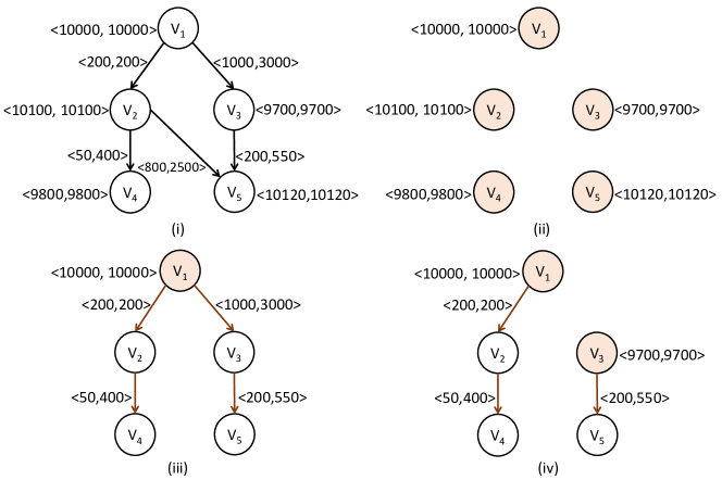
Figure 1: (i) A version graph over 5 datasets – annotation ⟨a, b⟩ indicates a storage cost of $a$ and a retrieval cost of $b$; (ii, iii, iv) three possible storage graphs. The figure is taken from [15]

This retrieval/storage trade-off leads to combinatorial problems of minimizing one type of cost, given a constraint on the other. Moreover, as an objective function, the retrieval cost can be measured by either the maximum or total (or equivalently average) retrieval cost of files. This yields four different optimization problems (Problems 3-6 in Table 1). While the first two problems in the table are easy, the other four turn out to be NP-hard and hard to approximate, as we will soon discuss.

Problem Name	Storage	Retrieval
Minimum Spanning Tree	min	$R(v)<\infty,\leavevmode\nobreak\ \forall v$
Shortest Path Tree	$<\infty$	min $\{\max_{\_}{v}R(v)\}$
MinSum Retrieval (MSR)	$\leq\mathcal{S}$	min$\{\sum_{\_}{v}R(v)\}$
MinMax Retrieval (MMR)	$\leq\mathcal{S}$	min $\{\max_{\_}{v}R(v)\}$
BoundedSum Retrieval (BSR)	min	$\sum_{\_}vR(v)\leq\mathcal{R}$
BoundedMax Retrieval (BMR)	min	$\max_{\_}vR(v)\leq\mathcal{R}$

Table 1: Problems 1-6. Here, $R(v)$ is the retrieval cost of version $v$, while $\mathcal{R},\mathcal{S}$ are the retrieval and storage constraints, respectively.

There are some follow-up works on this model [85, 28, 46]. However, those either formulate new problems in different use cases [28, 67, 46] or implement a system incorporating the feature to store specific versions and deltas [46, 82, 74]. We will discuss this in more detail in Section 1.2.

1.1 Our Contributions

We provide the first set of approximation algorithms and inapproximability results for the aforementioned optimization problems under various conditions. Our theoretical results also give rise to practical algorithms which perform very well on real-world data.

Problem	Graph type	Assumptions	Inapproximability
MSR	arborescence	Triangle inequality $r=s$ on edges	1
	undirected		$1+\frac{1}{e}-\epsilon$
	general		$\Omega(n)$
MMR	undirected		$2-\epsilon$
	general		$\log^{*}n-\omega(1)$
BSR	arborescence		1
	undirected		$(\frac{1}{2}-\epsilon)\log n$
BMR	undirected		$(1-\epsilon)\log n$

Table 2: Hardness results

MMR and BMR.

In Section 3 we prove that it is hard to approximate MMR within $\log^{*}n$ factor and BMR within $\log n$ factor on general inputs. Meanwhile, in LABEL:sec:MMRBMR we give a polynomial-time dynamic programming (DP) algorithm for the two problems on bidirectional trees, i.e., digraphs whose underlying undirected graph is a tree. These inputs capture the cases where new versions are generated via edit operations.

We also briefly describe an FPTAS (defined below) for MMR, analogous to the main result for MSR in LABEL:sec:fptas.

MSR and BSR.

In Section 3 we prove that it is hard to design $\big{(}O(n),O(\log n)\big{)}$-bicriteria approximation for MSR or $O(\log n)$-approximation for BSR. It is also NP-hard to solve the two problems exactly on trees.

On the other hand, we again use DP to design a fully polynomial-time approximation scheme (FPTAS) for MSR on bounded treewidth graphs. These inputs capture many practical settings: bidirectional trees have width 1, series-parallel graphs have width 2, and the GitHub repositories we use in (Section 5) all have low treewidth.

New Heuristics.

We improved LMG into a more general LMG-All algorithm for solving MSR. LMG-All outperforms LMG in all our experiments and runs faster than LMG on sparse graphs.

Inspired by our algorithms on trees, we also propose two DP heuristics for MSR and BMR. Both algorithms perform extremely well even when the input graph is not tree-like. Moreover, there are known procedures for parallelizing general DP algorithms [79], so our new heuristics are potentially more practical than previous ones, which are all sequential.

Graphs	Problems	Algorithm	Approx.
General Digraph	MSR	LMG-All	heuristic
Bounded Treewidth	MSR & MMR	DP-BTW	$1+\epsilon$
	BSR & BMR		$(1,1+\epsilon)$
Bidirectional Tree	MMR	DP-BMR	exact
	BMR

Table 3: Algorithms summary.

1.2 Related Works

1.2.1 Theory

There was little theoretical analysis of the exact problems we study. The optimization problems are first formalized in Bhattacherjee et al. [15], which also compared the effectiveness of several proposed heuristics on both real-world and synthetic data. Zhang et al.[85] followed up by considering a new objective that is a weighted sum of objectives in MSR and MMR. They also modified the heuristics to fit this objective. There are similar concepts, including Light Approximate Shortest-path Tree (LAST) [55] and Shallow-light Tree (SLT) [59, 45, 44, 68, 72, 54]. However, this line of work focuses mainly on undirected graphs and their algorithms do not generalize to the directed case. Among the two problems mentioned, SLT is closely related to MMR and BMR. Here, the goal is to find a tree that is light (minimize weight) and shallow (bounded depth). To our knowledge, there are only two works that give approximation algorithms for directed shallow-light trees. Chimani and Spoerhase [25] give a bi-criteria $(1+\epsilon,n^{\epsilon})$-approximation algorithm that runs in polynomial-time. Recently, Ghuge and Nagarajan [41] gave a $O(\frac{\log n}{\log\log n})$-approximation algorithm for submodular tree orienteering that runs in quasi-polynomial time. Their algorithm can be adapted into $O(\frac{\log^{2}n}{\log\log n})$-approximation for BMR. For MSR, their algorithm gives $\big{(}O(\frac{\log^{2}n}{\log\log n}),O(\frac{\log^{2}n}{\log\log n})\big{)}$-approximation. The idea is to run their algorithm for many rounds, where the objective of each round is to cover as many nodes as possible.

1.2.2 Systems

To implement a system captured by our problems, components spanning multiple lines of works are required. For example, to get a graph structure, one has to keep track of history of changes. This is related to the topic of data provenance [21, 77]. Given a graph structure, the question of modeling “deltas” is also of interest. There is a line of work dedicated to studying how to implement diff algorithms in different contexts [47, 22, 83, 65, 80].

In the more flexible case, one may think of creating deltas without access to the change history. However, computing all possible deltas is too wasteful, hence it is necessary to utilize other approaches to identify similar versions/datasets. Such line of work is known as dataset discovery or dataset similarlity [71, 50, 35, 19, 18].

Several follow-up works of Bhattacherjee et al.[15] have implemented systems with a feature that saves only selected versions to reduce redundancy. There are works focusing on version control for relational databases [20, 46, 74, 82, 23, 66, 14, 75] and works focusing on graph snapshots [84, 56, 67]. However, since their focus was on designing full-fledged systems, the algorithms they proposed are rather simple heuristics with no theoretical guarantees.

1.2.3 Usecases

In a version control system such as git, our problem is similar to what git pack command aims to do. The original heuristic for git pack, as described in an IRC log, is to sort objects in particular order and only create deltas between objects in the same window. It is shown in Bhattacherjee et al. [15] that git’s heuristic does not work well compared to other methods.

SVN, on the other hand, only stores the most recent version and the deltas to past versions [70]. Other existing data version management systems include [2, 3, 5, 6, 4], which offer git-like capabilities suited for different use cases, such as data science pipelines in enterprise setting, machine learning-focused, data lake storage, graph visualization, etc.

Though not directly related to our work, recently, there has been a lot of work exploring algorithmic and systems related optimizations for reducing storage and maintenance costs of data. For example, Mukherjee et al. [69] proposes optimal multi-tiering, compression and data partitioning, along with predicting access patterns for the same. Other works that exploit multi-tiering to optimize performance include e.g., [60, 29, 30, 24] and/or costs, e.g., [24, 32, 63, 64, 76, 57]. Storage and data placement in a workload aware manner, e.g., [7, 8, 24] and in a device aware manner, e.g., [81, 61, 62] have also been explored. [29] combine compression and multi-tiering for optimizing latency.

2 Preliminaries

In this section, the definition of the problems, notations, simplifications, and assumptions will be formally introduced.

2.1 Problem Setting

In the problems we study, we are given a directed version graph $G=(V,E)$, where vertices represent versions and edges capture the deltas between versions. Every edge $e=(u,v)$ is associated with two weights: storage cost $s_{\_}e$ and retrieval cost $r_{\_}e$. The cost of storing $e$ is $s_{\_}e$, and it takes $r_{\_}e$ time to retrieve $v$ once we retrieved $u$. Every vertex $v$ is associated with only the storage cost, $s_{\_}v$, of storing (materializing) the version. Since there is usually a smallest unit of cost in the real world, we will assume $s_{\_}v,s_{\_}e,r_{\_}e\in\mathbb{N}$ for all $v\in V,e\in E$.

To retrieve a version $v$ from a materialized version $u$, there must be some path $P=\{(u_{\_}{i-1},u_{\_}i)\}_{\_}{i=1}^{n}$ with $u_{\_}0=u,u_{\_}n=v$, such that all edges along this path are stored. In such cases, we say that $v$ is retrieved from materialized $u$ with retrieval cost $R(v)=\sum_{\_}{i=1}^{n}r_{\_}{(u_{\_}{i-1},u_{\_}i)}$. In the rest of the paper, we say $v$ is “retrieved from $u$” if $u$ is in the path to retrieve $v$, and $v$ is “retrieved from materialized $u$” if in addition $u$ is materialized.

The general optimization goal is to select vertices $M\subseteq V$ and edges $F\subseteq E$ of small size (w.r.t. storage cost $s$), such that for each $v\in V\setminus M$, there is a short path (w.r.t retrieval cost $r$) from a materialized vertex to $v$. Formally, we want to minimize (a) total storage cost $\sum_{\_}{v\in M}s_{\_}v+\sum_{\_}{e\in F}s_{\_}e$, and (b) total (resp. maximum) retrieval cost $\sum_{\_}{v\in V}R(v)$ (resp. $\max_{\_}{v\in V}R(v)$).

Since the storage and retrieval objectives are negatively correlated, a natural problem is to constrain one objective and minimize the other. With this in mind, four different problems are formulated, as described by Problems 3-6 in Table 1. These problems are originally defined in Bhattacherjee et al. [15], although we use different names for brevity. Since the first two problems are well studied, we do not discuss them further.

2.2 Further Definitions

We hereby formalize several simplifications and complications, to capture more realistic aspects of the problem. Most of the proposed variants are natural and considered by Bhattacherjee et al. [15].

Triangle inequality:

It is natural to assume that both weights satisfy triangle inequality, i.e., $r_{\_}{u,v}\leq r_{\_}{u,w}+r_{\_}{w,v}$, since we can always implement the delta $r_{\_}{u,v}$ by implementing first $r_{\_}{u,w}$ and then $r_{\_}{w,v}$.

In fact, a more general triangle inequality should hold when we consider the materialization costs $s_{\_}v$, as it’s often true that $s_{\_}u+s_{\_}{u,v}\geq s_{\_}v$ for all pairs of $u,v\in V$.

All hardness results in this paper hold under the generalized triangle inequality.

Directedness:

It is possible that for two versions $u$ and $v$, $r_{\_}{u,v}\neq r_{\_}{v,u}$. In real world, deletion is also significantly faster and easier to store than addition of content. Therefore, Bhattacherjee et al. [15] considered both directed and undirected cases; we argue that it is usually more natural to model the problems as directed graphs and focus on that case. Note that in the most general directed setting, it is possible that we are given the delta $(u,v)$ but not $(v,u)$. (For our purposes, this is equivalent to having a worse-than-trivial delta, with $s_{\_}{v,u}\geq s_{\_}u$.)

Directed and undirected cases are considered separately in our hardness results, and all our algorithms apply in the more general directed case.

Single weight function:

This is the special case where the storage cost function $s_{\_}e$ and retrieval cost $r_{\_}e$ function are identical up to some scaling. This can be seen in the real world, for example, when we use simple diff to produce deltas. We note that the random compression construction in our experiments (Section 5) is designed to simulate two distinct weight functions.

All our hardness results hold for single weight functions. All our approximation algorithms work even when the two weight functions are very different.

Arborescence and trees:

An arborescence, or a directed spanning tree, is a connected digraph where all vertices except a designated root have in-degree 1, and the root has in-degree 0. If each version is a modification on top of another version, then the “natural" deltas automatically form an arboreal input instance. For practical reasons, we also consider bidirectional tree instances, meaning that both $(u,v)$ and $(v,u)$ are available deltas with possibly different weights. Empirical evidence shows that having deltas in both directions can greatly improve the quality of the optimal solution.

Bounded treewidth:

At a high level, treewidth measures how similar a graph is to a tree [13]. As one notable class of graphs with bounded treewidths, series-parallel graphs highly resemble the version graphs we derive from real-world repositories. Therefore, graphs with bounded treewidth is a natural consideration with high practical utility. We give precise definitions of this special case in LABEL:subsec:DPBoundedTW.

We note that once we have an algorithm for MSR (resp. MMR), we can turn it into an algorithm for BSR (resp. BMR) by binary-searching over the possible values of the constraint. Due to the somewhat exchangeable nature of the storage and constraints in these problems, it’s worth considering $(\alpha,\beta)$-bicriteria approximations, where we relax the constraint by some $\beta$ factor in order to achieve a $\alpha$-approximation. For example, an algorithm $A$ is $(\alpha,\beta)$-bicriteria approximation for MSR if it outputs a feasible solution with storage cost $\leq\alpha\cdot\mathcal{S}$ and retrieval cost $\leq\beta\cdot OPT$ where $OPT$ is the retrieval cost of an optimal solution.

3 Hardness Results

We hereby prove the main hardness results of the problems. For completeness, we define the notion of approximation algorithms, as used in this paper, in Appendix A. We also include in Appendix B a list of well-studied optimization problems that are used in this section for reduction purposes.

3.1 Heuristics can be Arbitrarily Bad

First, we consider the approximation factor of the best heuristic for MSR in Bhattacherjee et al. [15], Local Move Greedy (LMG). The gist of this algorithm is to start with the arborescence that minimizes the storage cost, and iteratively materialize a version that most efficiently reduces retrieval cost per unit storage. In other words, in each step, a version is materialized with maximum $\rho$, where

$$\rho=\frac{\text{ reduction in total of retrieval costs}}{\text{increase in storage cost}}.$$

We provide the pseudocode for LMG in Algorithm 1.

Input :  Version graph $G$, storage constraint $\mathcal{S}$

/* Constructing extended version graph with auxiliary root $v_{\_}{aux}$. */

1 $V\leftarrow V\cup\{v_{\_}{aux}\}$;

2 for $v\in V\setminus\{v_{\_}{aux}\}$ do

3       $E\leftarrow E\cup\{(v_{\_}{aux},v)\}$;

4       $r_{\_}{(v_{\_}{aux},v)}=0$;

5       $s_{\_}{(v_{\_}{aux},v)}=s_{\_}v$;

6      

7Let $G_{\_}{aux}=(V,E)$;

/* The main algorithm. */

8 $T\leftarrow$ minimum arborescence of $G_{\_}{aux}$ rooted at $v_{\_}{aux}$ w.r.t. weight function $s$;

9 Let $S(T)$ be the total storage cost of $T$;

10 Let $R(v)$ be the retrieval cost of $v$ in $T$;

11 Let $P(v)$ be the parent of $v$ in $T$;

12 $U\leftarrow V$;

13 while $S(T)<\mathcal{S}$ do

14       $(\rho_{\_}{max},v_{\_}{max})\leftarrow(0,\varnothing)$;

15       for $v\in U$ with $S(T)+s_{\_}v-s_{\_}{P(v),v}\leq\mathcal{S}$ do

16             $T^{\prime}\leftarrow T\setminus\{(P(v),v)\}\cup\{(v_{\_}{aux},v)\}$;

17             $\Delta=\sum_{\_}v\big{(}R(v)-R_{\_}{T^{\prime}}(v)\big{)}$;

18             if $\Delta/(s_{\_}v-s_{\_}{P(v),v})>\rho_{\_}{max}$ then

19                   $\rho_{\_}{max}\leftarrow\Delta/(s_{\_}v-s_{\_}{P(v),v})$;

20                   $v_{\_}{max}\leftarrow v$;

21                  

22            

23      $T\leftarrow T\setminus\{(P(v_{\_}{max}),v_{\_}{max})\}\cup\{(v_{\_}{aux},v_{\_}{max})\}$;

24       $U\leftarrow U\setminus\{v_{\_}{max}\}$;

25       if $U=\varnothing$ then

26             return $T$;

27            

28      

29return $T$;

Algorithm 1 Local Move Greedy (LMG)

Theorem 3.1.

LMG has an arbitrarily bad approximation factor for MinSum Retrieval, even under the following assumptions:

$G$ is a directed path;

there is a single weight function; and

triangle inequality holds.

Proof 3.2.

Consider the following chain of three nodes; the storage costs for nodes and the storage/retrieval costs for edges are labeled in Figure 2 Let $a$ be large and $\epsilon=b/c$ be arbitrarily small. To save space, we do not show $v_{\_}{aux}$ but only the nodes of the version graph.

Figure 2: An adversarial example for LMG.

It is easy to check that triangle inequality holds on this graph.

In the first step of LMG, the minimum storage solution of the graph is $\{A,(A,B),(B,C)\}$ with storage cost $a+(1-\epsilon)b+(1-\epsilon)c$.

Next, in the greedy step, two options are available:

Choosing $B$ and delete $(A,B)$:

$$\rho_{\_}1=\frac{2(1-\epsilon)b}{\epsilon b}=\frac{2}{\epsilon}-1.$$

Choosing $C$ and delete $(B,C)$:

$$\rho_{\_}2=\frac{(1-\epsilon)b+(1-\epsilon)c}{\epsilon c}=\frac{(1-\epsilon)b}{b}+\frac{1-\epsilon}{\epsilon}=\frac{1}{\epsilon}-\epsilon<\frac{2}{\epsilon}-1.$$

With any storage constraint in range $\big{[}a+(1-\epsilon)b+c,a+b+c\big{)}$, LMG will choose Option 3.2 which gives a total retrieval cost of $(1-\epsilon)c$. Note that with $\mathcal{S}<a+b+c$, LMG is not able to pick Option 3.2 after taking Option 3.2. However, by choosing Option 3.2, which is also feasible, the total retrieval cost is $(1-\epsilon)b$. The proof is finished by observing that $c/b$ can be arbitrarily large.

3.2 Hardness Results on General Graphs

Here, we show the various hardness of approximations on general input graphs. We first focus on MSR and MMR where the constraint is on storage cost and the objective is on the retrieval cost. We then shift our attention to BMR and BSR in which the constraint is of retrieval cost and the objective function is on minimizing storage cost.

3.2.1 Hardness for MSR and MMR

Theorem 3.3.

On version graphs with $n$ nodes, even assuming single weight function and triangle inequality, there is no:

$(\alpha,\beta)$-approximation for MinSum Retrieval if $\beta\leq\frac{1}{2}(1-\epsilon)\big{(}\ln n-\ln\alpha-O(1)\big{)}$; in particular, for some constant $c$, there is no $(c\cdot n)$-approximation without relaxing storage constraint by some $\Omega(\log n)$ factor, unless $\textsc{NP}\subseteq\textsc{DTIME}(n^{O(\log\log n)})$;

$(1+\frac{1}{e}-\epsilon)$-approximation for MinSum Retrieval on undirected graphs for all $\epsilon>0$, unless $\textsc{NP}\subseteq\textsc{DTIME}(n^{O(\log\log n)})$;

$\big{(}\log^{*}(n)-\omega(1)\big{)}$-approximation for MinMax Retrieval, unless $\textsc{NP}\subseteq\textsc{DTIME}(n^{O(\log\log n)})$;

$(2-\epsilon)$-approximation for MinMax Retrieval on undirected graphs for all $\epsilon>0$, unless $\textsc{NP}=$P.

Proof 3.4.

MSR. There is an approximation-preserving (AP) reduction from (Asymmetric) k-median to MSR. Let $s_{\_}{u,v}=r_{\_}{u,v}=d_{\_}{u,v}$, the distance from $u$ to $v$ in a (asymmetric) $k$-median instance. By setting the size of each version $v$ to some large $N$ and storage constraint to be $\mathcal{S}=kN+n$, we can restrict the instance to materialize at most $k$ nodes and retrieve all other nodes through deltas. For large enough $N$, an $(\alpha,\beta)$-approximation for MSR provides an $(\alpha,\beta)$-approximation for (Asymmetric) k-median, just by outputting the materialized nodes. The desired results follow from known hardness for asymmetric [9] or symmetric (see Appendix B) k-median.

MMR. A similar AP reduction exists from (Asymmetric) k-center to MMR. Again, we can set all materialization costs to $N$ and $c_{\_}{u,v}=r_{\_}{u,v}=d_{\_}{u,v}$, and the desired result follows from the hardness of asymmetric [26] and symmetric [42] k-center.

3.2.2 Hardness for BSR and BMR

Theorem 3.5.

On both directed and undirected version graphs with $n$ nodes, even assuming single weight function and triangle inequality, there is no:

$(c_{\_}1\ln n)$-approximation for BoundedSum Retrieval for any $c_{\_}1<0.5$;

$(c_{\_}2\ln n)$-approximation for BoundedMax Retrieval for any $c_{\_}2<1$. unless $\textsc{NP}=\textsc{P}$.

To prove this theorem, we will present our reduction to these two problems from Set Cover. We then show their structural properties on Lemmas 3.6 and 3.8. We finally show the proof at the end of this section.

Reduction.

Given a set cover instance with sets $A_{\_}1,\ldots,A_{\_}m$ and elements $o_{\_}1,\ldots,o_{\_}n$, we construct the following version graph:

1. Build versions $a_{\_}i$ corresponding to $A_{\_}i$, and $b_{\_}j$ corresponding to $o_{\_}j$. All versions have size $N$ for some large $N\in\mathbb{N}$.

2. For all $i,j\in[m],i\neq j$, create symmetric delta $(a_{\_}i,a_{\_}j)$ of weight $1$. For each $o_{\_}j\in A_{\_}i$, create symmetric delta $(a_{\_}i,b_{\_}j)$ of weight $1$.

Lemma 3.6 (BMR’s structure).

Assume we are given an approximate solution to BMR on the above instance under max retrieval constraint $\mathcal{R}=1$. In polynomial time, we can produce another feasible solution with equal or smaller total storage cost such that only the set versions are materialized. i.e., all $\{b_{\_}j\}_{\_}{j=1}^{n}$ are retrieved via deltas.

Proof 3.7 (Proof of Lemma 3.6).

Suppose some algorithm produces a solution that materializes $b_{\_}j$.

Case 1:

If there exists $a_{\_}i$ that needs to be retrieved through $b_{\_}j$ (i.e., $o_{\_}j\in A_{\_}i$), then we can replace the materialization of $b_{\_}j$ with that of $a_{\_}i$ and replace edges of the form $(b_{\_}j,a_{\_}k)$ with $(a_{\_}i,a_{\_}k)$. It is straightforward to see that neither storage cost nor retrieval cost increased in this process.

Case 2:

If no other node is dependent on $b_{\_}j$, we can pick any $a_{\_}i$ such that $(a_{\_}i,b_{\_}j)$ exists (again, $o_{\_}j\in A_{\_}i$). If $a_{\_}i$ is already materialized in the original solution, then we can store $(a_{\_}i,b_{\_}j)$ instead of materializing $b_{\_}j$, which decreases storage cost.

Case 3:

If no $a_{\_}i$ adjacent to $b_{\_}j$ is materialized in the original solution, then some delta $(a_{\_}{i^{\prime}},a_{\_}i)$ has to be stored with the former materialized to satisfy the $\mathcal{R}=1$ constraint. We can hence materialize $a_{\_}i$, delete the delta $(a_{\_}{i^{\prime}},a_{\_}i)$, and again replace the materialization of $b_{\_}j$ with the delta $(a_{\_}i,b_{\_}j)$ without increasing the storage. Figure 3 illustrates this case.

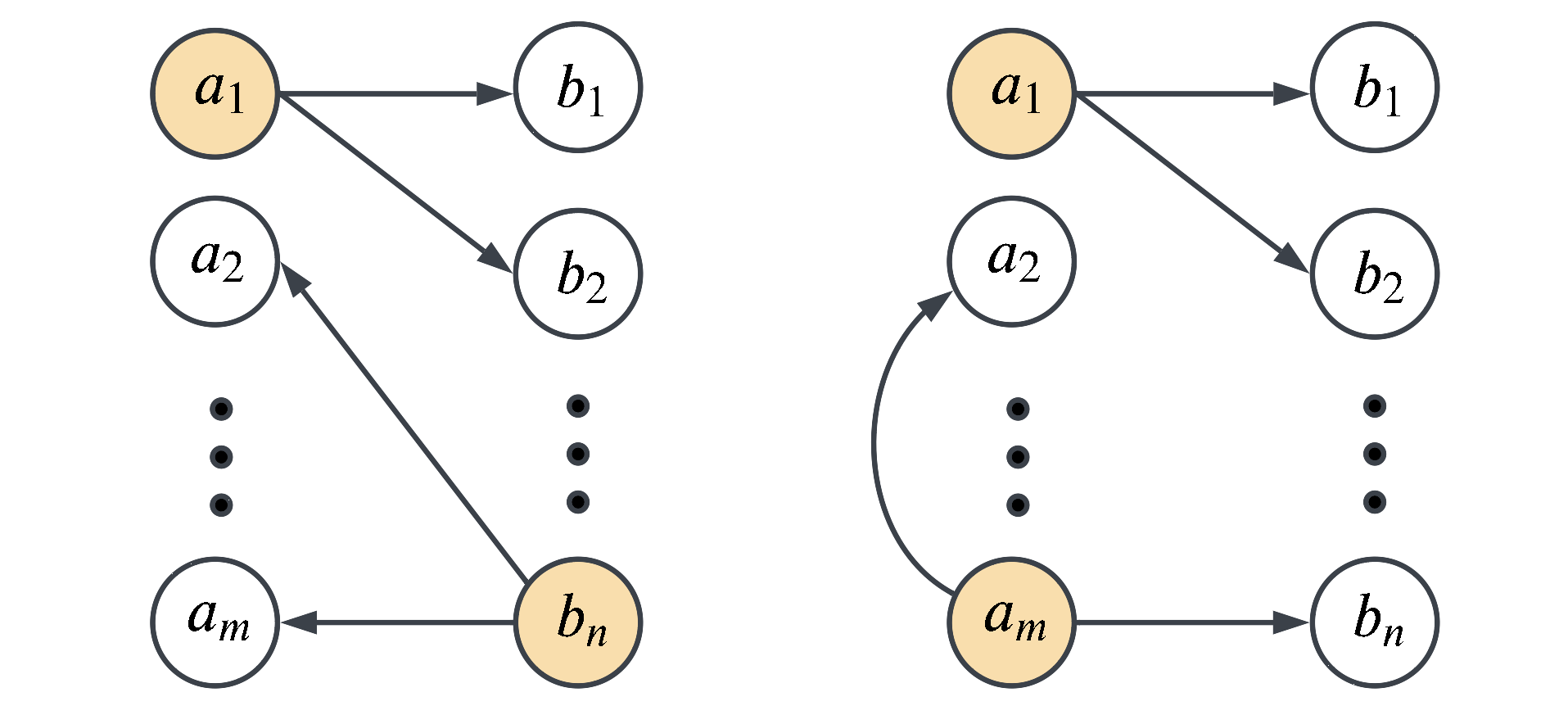
Figure 3: Case 3 in the proof of Lemma 3.6. The improved solution is on the right.

Lemma 3.8 (BSR’s structure).

Assume we are given an approximate solution to BSR on the above version graph under total retrieval constraint $\mathcal{R}=m-m_{\_}{\text{OPT}}+n$, where $m_{\_}{\text{OPT}}$ is the size of the optimal set cover. In polynomial time, we can produce another feasible solution to BSR with equal or lower total storage cost, such that only the set versions are materialized. i.e., all $\{b_{\_}j\}_{\_}{j=1}^{n}$ are retrieved via deltas.

Proof 3.9 (Proof of Lemma 3.8).

We refer to the same three cases as in Lemma 3.6. Similarly, if we have a solution where some $b_{\_}j$ is materialized,

Case 1:

if some $a_{\_}i$ is retrieved through $b_{\_}j$, we can apply the same modification as Lemma 3.6. We can replace the materialization of $b_{\_}j$ with that of $a_{\_}i$, and replace edges of the form $(b_{\_}j,a_{\_}k)$ with $(a_{\_}i,a_{\_}k)$. Neither the storage nor the retrieval cost increases in this case.

Now, WLOG we assume no deltas $(b_{\_}j,a_{\_}i)$ are chosen.

Case 2:

if no $a_{\_}i$ is retrieved through $b_{\_}j$, and some $a_{\_}i$ adjacent to $b_{\_}j$ is materialized, then method in Lemma 3.6 needs to be modified a bit in order to remove the materialization of $b_{\_}j$. If we simply retrieve $b_{\_}j$ via the delta $(a_{\_}i,b_{\_}j)$, we would lower the storage cot by $N-1$ and increase the total retrieval cost by $1$. This renders the solution infeasible if the total retrieval constraint is already tight.

To tackle this, we analyze the properties of the solutions with total retrieval cost exactly $\mathcal{R}$. Observe that all solutions must materialize at least $m_{\_}{\text{OPT}}$ nodes at all time, so a configuration exhausting the constraint $R$ must have some version $w$ with retrieval cost at least $2$. If this $w$ is a set version, we can loosen the retrieval constraint by storing a delta of cost 1 from some materialized set instead. If $w$ is an element version, then we can materialize its parent version (a set covering it), which increases storage cost by $N-1$ and decreases total retrieval cost by at least 2.

Either case, by performing the above action if necessary, we can resolve case 2 and obtain a approximate solution that is not worse than before.

Case 3:

this is where each $a_{\_}i$ adjacent to $b_{\_}j$ neither retrieves through $b_{\_}j$ nor is materialized. Fix an $a_{\_}i$, then some delta $(a_{\_}{i^{\prime}},a_{\_}i)$ has to be stored to retrieve $a_{\_}i$; WLOG we can assume that the former is materialized. We can thus materialize $a_{\_}i$, delete the delta $(a_{\_}{i^{\prime}},a_{\_}i)$, and again replace the materialization of $b_{\_}j$ with the delta $(a_{\_}i,b_{\_}j)$ with no increase in either costs.

Equipped with Lemma 3.6 and Lemma 3.8, we are now ready to prove Theorem 3.5.

Proof 3.10 (Proof of Theorem 3.5).

Assuming $m=O(n)$ in the set cover instance, we present an AP reduction from Set Cover to both BMR and BSR.

BMR.

To produce a set cover solution, we take an improved approximate solution for BMR, and output the family of sets whose corresponding versions are materialized. Since none of the $b_{\_}j$’s is stored, they have to be retrieved from some $a_{\_}i$. Moreover, under the constraint $\mathcal{R}=1$, they have to be a 1-hop neighbor of some $a_{\_}i$, meaning the materialized $a_{\_}i$ covers all of the elements in the set cover instance.

Finally, we prove that the approximation factor is preserved: for large $N$, the improved solution has objective value $\approx N|\{i:a_{\_}i\text{ materialized}\}|.$ If $n=O(m)$, then an $\alpha(|V|)$-approximation for MMR provides a $(\alpha(n)+O(1))$-approximation for set cover. Hence we can not have $\alpha(|V|)=c\ln n$ for $c<1$ unless $\textsc{NP}\subseteq\textsc{DTIME}(n^{O(\log\log n)})$ [33].

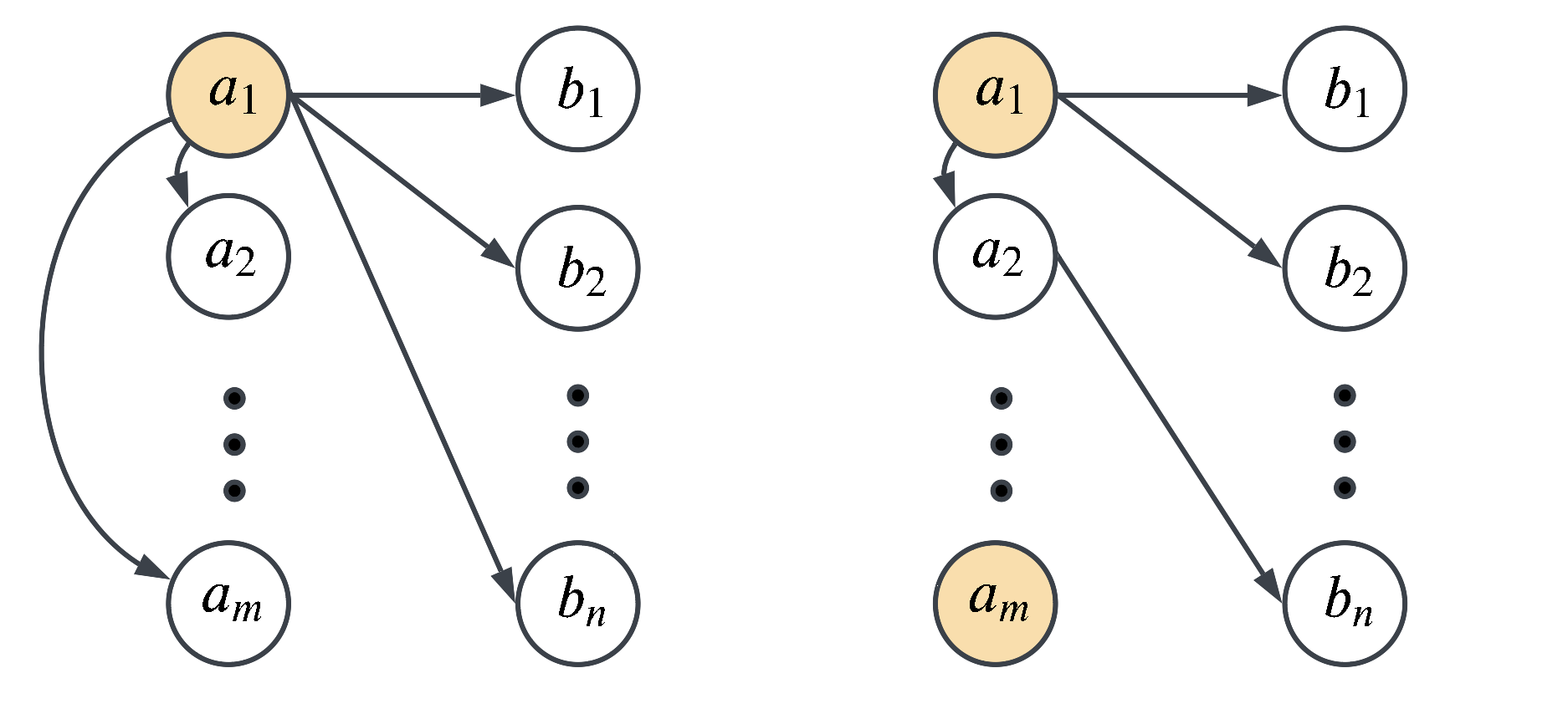
Figure 4: The BSR case in proof of Theorem 3.5. The solution on the right has one version ($b_{\_}2$) of retrieval cost 2, hence it must materialize an additional version $a_{\_}m$ to satisfy the total retrieval constraint.

BSR.

Assume for the moment that we know $m_{\_}{\text{OPT}}$, then we can set total retrieval constraint to be $\mathcal{R}=m-m_{\_}{\text{OPT}}+n$, and work with an improved approximate solution. This choice of $\mathcal{R}$ is made so that an optimal solution must materialize the set versions corresponding to a minimum set cover. All other nodes must be retrieved via a single hop.

By Lemma 3.8, we assume all element versions are retrieved from a (not necessarily materialized) set version that covers it. If $m=O(n)$, an $\alpha(|V|)$-approximation of BMR materializes $m_{\_}{\text{ALG}}\leq(\alpha(n)+O(1))m_{\_}{\text{OPT}}$ nodes.

Note that, by materializing additional nodes, we are allowing a set $B$ of $b_{\_}j$’s to have retrieval cost $\geq 2$. Let $H$ denote the set of “hopped sets” $A_{\_}i$, which are not materialized yet are necessary to retrieve some $b_{\_}j$ through the delta $(a_{\_}i,b_{\_}j)$. By analyzing the total retrieval cost, we can bound $|H|$ by:

$$|H|\leq|B|\leq m_{\_}{\text{ALG}}-m_{\_}{\text{OPT}}$$

Specifically, each additional $b_{\_}j\in B$ increases retrieval cost by at least $1$ compared to the optimal configuration; yet each of the $m_{\_}{\text{ALG}}-m_{\_}{\text{OPT}}$ additionally materialized set versions only decreases total retrieval cost by 1. It follows that the family of sets

$$S=\{A_{\_}i:a_{\_}i\text{ materialized }\}\cup H$$

is a $\Big{(}2\alpha(n)-O(1)\Big{)}$-approximation solution for the corresponding Set Cover instance. $S$ is feasible because all of the $b_{\_}j$’s are retrieved through some $(a_{\_}i,b_{\_}j)$, where $A_{\_}i\in S$; on the other hand, the size of both sets on the right hand side are at most $(\alpha(n)+O(1))m_{\_}{\text{OPT}}$, hence the approximation factor holds. Thus, any $\alpha(|V|)=c\ln n$ for any $c<0.5$ will result in a Set Cover approximation factor of $2c\cdot\ln(n)$.

We finish the proof by noting that, without knowing $m_{\_}{\text{OPT}}$ in advance, we can run the above procedure for each possible guess of the value $m_{\_}{\text{OPT}}$, and obtaining a feasible set cover each iteration. The desired approximation factor is still preserved by outputting the minimum set cover solution over the guesses.

3.3 Hardness on Arborescences

We show that MSR and BSR are NP-hard on arborescence instances. This essentially shows that our FPTAS algorithm for MSR in LABEL:subsec:tree-dp is the best we can do in polynomial time.

Theorem 3.11.

On arborescence inputs, MinSum Retrieval and BoundedSum Retrieval are NP-hard even when we assume single weight function and triangle inequality.

In order to prove the theorem above, we rely on the following reduction which connects two problems together.

Lemma 3.12.

If there exists poly-time algorithm $\mathcal{A}$ that solves BoundedSum Retrieval (resp. BoundedMax Retrieval) on some set of input instances, then there exists a poly-time algorithm solving MinSum Retrieval (resp. MinMax Retrieval) on the same set of input instances.

Proof 3.13.

Suppose we want to solve a MSR (resp. MMR) instance with storage constraint $\mathcal{S}$. We can use $\mathcal{A}$ as a subroutine and conduct binary search for the minimum retrieval constraint $\mathcal{R}^{*}$ under which BSR (resp. BMR) has optimal objective at most $\mathcal{S}$. Thus, $\mathcal{R}^{*}$ is an optimal solution for our problem at hand.

To see that the binary search takes poly$(n)$ steps, we note that the search space for the target retrieval constraint is bounded by $n^{2}r_{\_}{max}$ for BSR and $nr_{\_}{max}$ for BMR, where $r_{\_}{max}=\max_{\_}{e\in E}r_{\_}e$.

Now we show the proof for Theorem 3.11.

Proof 3.14 (Proof of Theorem 3.11).

Assuming Lemma 3.12, it suffices to show the NP-hardness of MSR on these inputs.

Consider an instance of Subset Sum problem with values $a_{\_}1,\ldots,a_{\_}n$ and target $T$. This problem can be reduced to MSR on an $n$-ary arborescence of depth one. Let the root version be $v_{\_}0$ and its children $v_{\_}1,\ldots,v_{\_}n$. The materialization cost of $v_{\_}i$ is set to be $a_{\_}i+1$ for $i\in[n]$, while that of $v_{\_}0$ is some $N$ large enough so that the generalized triangle inequality holds. For each $i\in[n]$, we can set both retrieval and storage costs of edge $(v_{\_}0,v_{\_}i)$ to be $1$.

Consider MSR on this graph with storage constraint $\mathcal{S}=N+n+T$. From an optimal solution, we can construct set $A=\{i\in[n]:v_{\_}i\text{ materialized}\}$, an optimal solution for the above Subset Sum instance.

4 Heuristics on MSR and BMR

In this section, we propose three new heuristics that are inspired by empirical observations and theoretical results.

4.1 LMG-All: Improvement over LMG

We propose an improved version of LMG (Algorithm 1), which we name LMG-All. (See Algorithm 2 for pseudocode.) LMG-All enlarges the scope of the search on each greedy step. Instead of searching for the most efficient version to materialize, we explore the payoff of modifying any single edge:

1. Find a configuration that minimizes total storage cost.

2. Let $\text{Par}(v)$ be the current parent of $v$ on retrieval path. In addition to $V_{\_}{active}$, Define edge set $E_{\_}{active}$ to be the edges that (a) does not cause the configuration to exceed storage constraint $\mathcal{S}$, and (b) does not form cycles, if $(u,v)\in E_{\_}{active}$ were to replace $(\text{Par}(v),v)$ in the current configuration. If $V_{\_}{active}=E_{\_}{active}=\varnothing$, output the current configuration.

3. Calculate cost and benefit of each $v\in V_{\_}{active}$ and $e\in E_{\_}{active}$. Materialize or store the most cost-effective node or edge. Go to step 2 and repeat.

Input : Version graph $G$, storage constraint $\mathcal{S}$

$G_{\_}{aux}\leftarrow$ extended version graph with auxiliary root. /* See Algorithm 1 for the construction of $G_{\_}{aux}$. */

1 $T\leftarrow$ minimum arborescence of $G_{\_}{aux}$ rooted at $v_{\_}{aux}$ with respect to weight function $s$;

2 Let $R(T)$ and $S(T)$ be the total retrieval and storage cost of $T$;

3 Let $P(v)$ be the parent of $v$ in $T$;

4 while $S(T)<\mathcal{S}$ do

5       $(\rho_{\_}{max},(u_{\_}{max},v_{\_}{max}))\leftarrow(0,\varnothing)$;

6       for $e=(u,v)\in E$ where $u$ is not a descendant of $v$ in $T$ do

7             $T_{\_}e=T\setminus(P(v),v)\cup\{e\}$;

8             if $R(T_{\_}e)>R(T)$ then

9                   continue;

10                  

11            if $S(T_{\_}e)\leq S(T)$ then

12                   $\rho_{\_}e\leftarrow\infty$;

13            else

14                   $\rho_{\_}{e}\leftarrow(R(T)-R(T_{\_}e))/(s_{\_}e-s_{\_}{P(v),v})$;

15            

16            if $\rho_{\_}e>\rho_{\_}{max}$ then

17                   $\rho_{\_}{max}\leftarrow\rho_{\_}e$;

18                   $(u_{\_}{max},v_{\_}{max})\leftarrow e$;

19                  

20            

21      if $\rho_{\_}{max}=0$ then

22             return $T$ ;

23            

24      

25      $T\leftarrow T\setminus\{(P(v_{\_}{max}),v_{\_}{max})\}\cup\{(u_{\_}{max},v_{\_}{max})\}$;

26      

27return $T$;

Algorithm 2 LMG-ALL

While LMG-All considers more edges than LMG, it is not obvious that LMG-All always provides a better solution, due to its greedy nature.

4.2 DP on Extracted Bidirectional Trees

We propose DP heuristics for both MSR and BMR, as inspired by algorithms in LABEL:Sec:arbor and LABEL:sec:fptas.

To ensure a reasonable running time, we extract bidirectional trees from input graphs and run the DP for treewidth 1 on the extracted graph, with the steps below:

Fix a node $v_{\_}{root}$ as the root. Calculate a minimum spanning arborescence $A$ of the graph $G$ rooted at $v_{\_}{root}$. We use the sum of retrieval and storage costs as weight.

Generate a bidirectional tree $G^{\prime}$ from $A$. Namely, we have $(u,v),(v,u)\in E(G^{\prime})$ for each edge $(u,v)\in E(A)$.

Run the proposed DP for MSR and BMR on directed trees (see LABEL:subsec:tree-dp and LABEL:sec:MMRBMR) with input $G^{\prime}$.

In addition, we also implement the following modifications for MSR to further speed up the algorithm:

1. Total storage cost (instead of retrieval) is discretized and used as DP variable index, since it has a smaller range than retrieval cost.

2. Geometric discretization is used instead of linear discretization, reducing the number of discretized “ticks.”

3. A pruning step is added, where the DP variable discards all subproblem solutions whose storage cost exceeds some threshold. This reduces redundant computations.

All three original features are necessary in the proof for our theoretical results, but in practice, the modified implementations show comparable results but significantly improves the running time.

5 Experiments for MSR and BMR

In this section, we discuss the experimental setup and results for empirical validation of the algorithms’ performance, as compared to previous best-performing heuristic: LMG for MSR, and MP for BMR.

In all figures, the vertical axis (objective and run time) is presented in logarithmic scale. Run time is measured in milliseconds.

5.1 Datasets and Construction of Graphs

As in Bhattacherjee et al [15], we conduct experiment on real-world GitHub repositories of varying sizes as datasets. We construct version graphs as follows. Each commit corresponds to a node with its storage cost equal to its size in bytes. Between each pair of parent and child commits, we construct bidirectional edges. The storage and retrieval costs of the edges are calculated, in bytes, based on the actions (such as addition, deletion, and modification of files) required to change one version to the other in the direction of the edge. We use simple diff to calculate the deltas, hence the storage and retrieval costs are proportional to each other. Graphs generated this way are called “natural graphs” in the rest of the section.

In addition, we also aim to test (1) the cases where the retrieval and storage costs of an edge can greatly differ from each other, and (2) the effect of tree-like shapes of graphs on the performance of algorithms. Therefore, we also conduct experiments on modified graphs in the following two ways:

Random compression.

We simulate compression of data by scaling storage cost with a rand om factor between 0.3 and 1, and increasing the retrieval cost by 20% (to simulate decompression). The resulting storage and retrieval costs are potentially very different.

Dataset	#nodes	#edges	avg. cost $s_{\_}v$	avg. cost $s_{\_}e$
datasharing	29	74	7672	395
styleguide	493	1250	$1.4\times 10^{6}$	8659
996.ICU	3189	9210	$1.5\times 10^{7}$	337038
freeCodeCamp	31270	71534	$2.5\times 10^{7}$	14800
LeetCodeAnimation	246	628	$1.7\times 10^{8}$	$1.2\times 10^{7}$
LeetCode (0.05)	246	3032	$1.7\times 10^{8}$	$1.0\times 10^{8}$
LeetCode (0.2)	246	11932	$1.7\times 10^{8}$	$1.0\times 10^{8}$
LeetCode (1)	246	60270	$1.7\times 10^{8}$	$1.0\times 10^{8}$

Table 4: Natural and ER graphs overview.

ER construction.

Instead of the naturally constructing edges between each pair of parent and child commits, we construct the edges as in an Erdős-Rényi random graph: between each pair $(u,v)$ of versions, with probability $p$ both deltas $(u,v)$ and $(v,u)$ are constructed, and with probability $1-p$ neither are constructed. The resulting graphs are much less tree-like. We construct ER graphs from the repository LeetCode because it has a moderate size and is the least tree-like.

5.2 Results in MSR

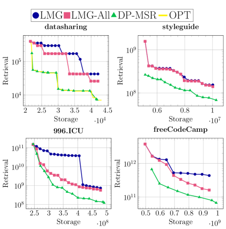
Figure 5: Performance of MSR algorithms on natural graphs. OPT is obtained by solving an integer linear program (ILP, see Appendix D) using Gurobi [43]. ILP takes too long to finish on all graphs except datasharing.

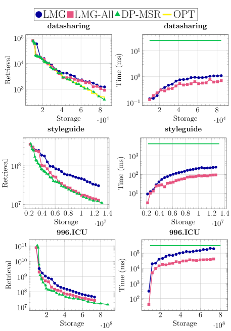
Figure 6: Performance and run time of MSR algorithms on compressed graphs.

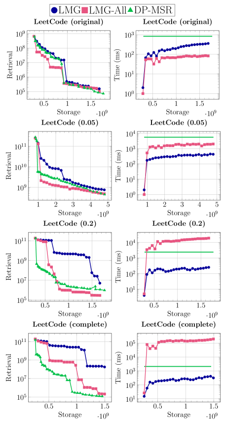
Figure 7: Performance and run time of MSR algorithms on compressed ER graphs.

Figure 5, Figure 6, and Figure 7 demonstrate the performance of the three MSR algorithms on natural graphs, compressed natural graphs, and compressed ER graphs. The running times for the algorithms are shown in Figure 6 and Figure 7. Since run time for most non-ER graphs exhibit similar trends, many are omitted here due to space constraint. Also note that, since DP-MSR generates all data points in a single run, its running time is shown as a horizontal line over the full range for storage constraint.

We run DP-MSR with $\epsilon=0.05$ on most graphs, except $\epsilon=0.1$ for freeCodeCamp (for the feasibility of run time). The pruning value for DP variables is at twice the minimum storage for uncompressed graphs, and ten times the minimum storage for randomly compressed graphs.

Performance analysis.

On most graphs, DP-MSR outperforms LMG-All, which in turn outperforms LMG. This is especially clear on natural version graphs, where DP-MSR solutions are near 1000 times better than LMG solutions on 996.ICU. in Figure 5. On datasharing, DP-MSR almost perfectly matches the optimal solution (calculated via the ILP in Appendix D) for all constraint ranges.

On naturally constructed graphs (Figure 5), LMG-All often has comparable performance with LMG when storage constraint is low. This is possibly because both algorithms can only iterate a few times when the storage constraint is almost tight. DP-MSR, on the other hand, performs much better on natural graphs even for low storage constraint.

On graphs with random compression (Figure 6), the dominance of DP in performance over the other two algorithms become less significant. This is anticipated because of the fact that DP only runs on a subgraph of the input graph. Intuitively, most of the information is already contained in a minimum spanning tree when storage and retrieval costs are proportional. Otherwise, the dropped edges may be useful. (They could have large retrieval but small storage, and vice versa. )

Finally, LMG’s performance relative to our new algorithms is much worse on ER graphs. This may be due to the fact that LMG cannot look at non-auxiliary edges once the minimum arborescence is initialized, and hence losing most of the information brought by the extra edges. (Figure 7).

Run time analysis.

For all natural graphs, we observe that LMG-All uses no more time than LMG (as shown in Figure 6). Moreover, LMG-All is significantly quicker than LMG on large natural graphs, which was unexpected considering that the two algorithms have almost identical structures in implementation. Possibly, this could be due to LMG making bigger, more expensive changes on each iteration (materializing a node with many dependencies, for instance) as compared to LMG-All.

As expected, though, LMG-All takes much more time than the other two algorithms on denser ER graphs (Figure 7), due to the large number of edges.

DP-MSR is often slower than LMG, except when ran on the natural construction of large graphs (Figure 6). However, unlike LMG and LMG-All, the DP algorithm returns a whole spectrum of solutions at once, so it is difficult to make a direct comparison. We also note that the run time of DP heavily depends on the choice of $\epsilon$ and the storage pruning bound. Hence, the user can trade-off the run time with solution’s qualities by parameterize the algorithm with coarser configurations.

5.3 Results in BMR

As compared to MSR algorithms, the performance and run time of our BMR algorithms are much more predictable and stable. They exhibit similar trends across different ways of graph construction as mentioned earlier in this section - including the non-tree-like ER graphs, surprisingly.

Due to space limitation, we only present the results on natural graphs, as shown in Figure 8, to respectively illustrate their performance and run time.

Performance analysis.

For every graph we tested, DP-BMR outperforms MP on most of the retrieval constraint ranges. As the retrieval constraint increases, the gap between MP and DP-BMR solution also increases. We also observe that DP-BMR performs worse than MP when the retrieval constraint is at zero. This is because the bidirectional tree have fewer edges than the original graph. (Recall that the same behavior happened for DP-MSR on compressed graphs)

We also note that, unlike MP, the objective value of DP-BMR solution monotonically decreases with respect to retrieval constraint. This is again expected since these are optimal solutions of the problem on the bidirectional tree.

Run time analysis.

For all graphs, the run times of DP-BMR and MP are comparable within a constant factor. This is true with varying graph shapes and construction methods in all our experiments, and representative data is exhibited in Figure 8. Unlike LMG and LMG-All, their run times do not change much with varying constraint values.

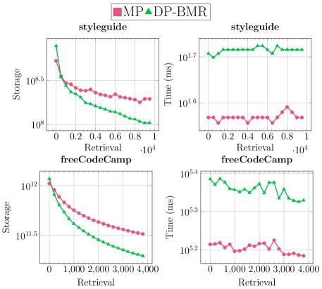
Figure 8: Performance and run time of BMR algorithms on natural version graphs.

Overall evaluation

For MSR, we recommend always using one of LMG-All and DP-MSR in place of LMG for practical use. On sparse graphs, LMG-All dominates LMG both in performance and run time. DP-MSR can also provide a frontier of better solutions in a reasonable amount of time, regardless of the input.

For BMR, DP-BMR usually outperforms MP, except when the retrieval constraint is close to zero. Therefore, we recommend using DP in most situations.

6 Conclusion

In this paper, we developed fully polynomial time approximation algorithms for graphs with bounded treewidth. This often captures the typical manner in which edit operations are applied on versions. For practical use, we extracted the idea behind this approach as well as previous LMG approach, and developed heuristics which significantly improved both the performance and run time in experiments, while potentially allowing for parallelization.

Appendix A Approximation Algorithms

We hereby define the notion of approximation algorithms used in this paper.

Definition A.1 ($\rho$-approximation algorithm).

Let $\mathcal{P}$ be a minimization problem where we want to come up with a feasible solution $x$ satisfying some constraints (e.g., $a\cdot x\leq b$). We say that an algorithm $\mathcal{A}$ is a $\rho$-approximation algorithm for $\mathcal{P}$ if $x_{\_}{\mathcal{A}}$, the solution produced by $\mathcal{A}$ is feasible and that $OPT\leq f(x_{\_}{\mathcal{A}})\leq\rho\cdot OPT$ where $OPT$ is an optimal objective value and $f(x)$ is the objective value of a solution $x$. Here, $\rho$ is the approximation ratio. Generally, we want $\mathcal{A}$ to run in polynomial time.

Definition A.2 (Polynomial-time approximation scheme (PTAS)).

A polynomial-time approximation scheme is an algorithm $\mathcal{A}$ that, when given any fixed $\epsilon>0$, can produce an $(1+\epsilon)$-approximation in time that is polynomial in the instance size. We say that $\mathcal{A}$ is a fully polynomial-time approximation scheme (FPTAS) if the runtime of $\mathcal{A}$ is polynomial in both the instance size and $1/\epsilon$.

Definition A.3 (Bi-criteria approximation).

In problems such as ours where optimizing an objective function while meeting all constraints is challenging, we can consider relaxing both aspects. We say that an algorithm $\mathcal{A}$ $(\alpha,\beta)$-approximates problem $\mathcal{P}$ if the objective value of its output is at most $\alpha$ times the objective value of an optimal solution and the constraints are violated at most $\beta$ times.

Appendix B Optimization Problems with Known Hardness Results

We hereby define a few problems with known hardness results that reduce to one of the versioning problems.

Before we show our hardness results, it is useful to introduce several other NP-hard problems to reduce from.

Definition B.1 (Set Cover).

Elements $U=\{o_{\_}1,\ldots,o_{\_}n\}$ and subsets $S_{\_}1,\ldots,S_{\_}m\subseteq U$ are given. The goal is to find $A\subseteq[m]$ with minimum cardinality such that $\bigcup_{\_}{i\in A}S_{\_}i=U$.

Set Cover has no $c\ln n$-approximation for any $c<1$, unless $\textsc{P}=\textsc{NP}$ [31].

Definition B.2 (Subset Sum).

Given real values $a_{\_}1,\ldots,a_{\_}n$ and a target value $T$. The goal is to find $A\subseteq[n]$ such that $\sum_{\_}{i\in A}a_{\_}i$ is maximized but not greater than $T$.

Subset Sum is also NP-hard, but its FPTAS is well studied [48, 52, 39, 40, 53].

Definition B.3 (k-median and Asymmetric k-median).

Given nodes $V=\{1,\ldots,n\}$, $k$, and symmetric (resp. asymmetric) distance measures $D_{\_}{i,j}$ for $i,j\in V$ that satisfies triangle inequality. The goal is to find a set of nodes $A\subseteq V$ of cardinality at most $k$ that minimizes

$$\sum_{\_}{v\in V}\min_{\_}{c\in A}D_{\_}{v,c}.$$

The symmetric problem is well studied. The best known approximation lower bound for this problem is $1+\frac{1}{e}$. We note that an inapproximability result of $1+\frac{2}{e}$ [49] is often mistakenly quoted for this problem, whereas the authors actually studied the $k$-median variant where the “facilities” and “clients” are in different sets. With the same method we can only get the hardness of $1+1/e$ in our definition.

The asymmetric counterpart is rarely studied. The manuscript  [9] showed that there is no $(\alpha,\beta)$-approximation ($\beta$ is the relaxation factor on $k$) if $\beta\leq\frac{1}{2}(1-\epsilon)(\ln n-\ln\alpha-O(1))$, unless $\textsc{NP}\subseteq\textsc{DTIME}(n^{O(\log\log n)})$.

Notably, even symmetric $k-$median is inapproximable when triangle inequality is not assumed on the distance measure $D$. [78] However, this hardness is not preserved by the standard reduction to MSR (as in Section 3.2.1), since the path distance on graphs inherently satisfies triangle inequality.

Definition B.4 (k-center and Asymmetric k-center).

Given nodes $V=\{1,\ldots,n\}$, $k$, and asymmetric distance measures $D_{\_}{i,j}$ for $i,j\in V$ that satisfies triangle inequality. The goal is to find a set of nodes $A\subseteq V$ of cardinality at most $k$ that minimizes

$$\max_{\_}{v\in V}\min_{\_}{c\in A}D_{\_}{v,c}.$$

The symmetric problem has a greedy 2-approximation, which is optimal unless P$=\textsc{NP}$ [42].

The asymmetric variant has $\log^{*}k$-approximation algorithms [10], and one cannot get a better approximation than $\log^{*}n$ unless $\textsc{NP}\subseteq\textsc{DTIME}(n^{O(\log\log n)})$, if we allow $k$ to be arbitrary [26].

Appendix C Reduction from General Trees to Binary Trees (Section LABEL:subsec:tree-dp)

Lemma C.1.

If algorithm $\mathcal{A}$ solves BMR on binary tree instances in $O(f(n))$ time where $n$ is the number of vertices in the tree, then there exists algorithm $\mathcal{A}^{\prime}$ solving BMR on all tree instances in $O(f(2n))$ time.

Proof C.2 (Proof Sketch).

If a node $v$ has more than two children, we modify the graph as follows:

Create node $v^{\prime}$ and attach it as a child of $v$.

Move all but the left-most children of $v$ to be children of $v^{\prime}$

Set the deltas of $(v,v^{\prime})=(v^{\prime},v)=0$; set $(v^{\prime},c_{\_}i)=(v,c_{\_}i)$ and $(c_{\_}i,v^{\prime})=(c_{\_}i,v)$ for all transferred children $c_{\_}i$. By repeating this process we obtain a binary tree with $\leq 2n$ nodes which has the same optimal objective value as before. Hence, after producing a binary tree, we can utilize the algorithm for binary tree to solve BMR on any tree.

$$S_{\_}1 =s_{\_}v$$

$$+\min_{\_}{\rho_{\_}1+\rho_{\_}2=\rho}\Big{\{}\min_{\_}{k_{\_}1,\gamma_{\_}1}\{DP[c_{\_}1][k_{\_}1][\gamma_{\_}2][\rho_{\_}1]\}+\min_{\_}{k_{\_}2,\gamma_{\_}2}\{DP[c_{\_}2][k_{\_}2][\gamma_{\_}2][\rho_{\_}2]\Big{\}}$$

$$S_{\_}2 =s_{\_}v+s_{\_}{v,c_{\_}1}-s_{\_}{c_{\_}1}$$

$$+\min_{\_}{\rho_{\_}1\leq\rho}\Big{\{}DP[c_{\_}1][k-1][0][\rho_{\_}1-(k-1)r_{\_}{v,c_{\_}1}]+\min_{\_}{k^{\prime},\gamma_{\_}2}\{DP[c_{\_}2][k^{\prime}][\gamma_{\_}2][\rho-\rho_{\_}1]\}\Big{\}}$$

$$S_{\_}3 =s_{\_}v+s_{\_}{v,c_{\_}2}-s_{\_}{c_{\_}2}$$

$$+\min_{\_}{\rho_{\_}1+\rho_{\_}2=\rho}\Big{\{}\min_{\_}{k^{\prime},\gamma_{\_}1}\{DP[c_{\_}1][k^{\prime}][\gamma_{\_}1][\rho_{\_}1]\}+DP[c_{\_}2][k-1][0][\rho_{\_}2-(k-1)r_{\_}{v,c_{\_}2}]\Big{\}}$$

$$S_{\_}4 =s_{\_}v+s_{\_}{v,c_{\_}1}-s_{\_}{c_{\_}1}+s_{\_}{v,c_{\_}2}-s_{\_}{c_{\_}2}$$

$$+\min_{\_}{\rho_{\_}1+\rho_{\_}2=\rho}\min_{\_}{k_{\_}1+k_{\_}2=k-1}\Big{\{}DP[c_{\_}1][k_{\_}1][0][\rho_{\_}1-k_{\_}1r_{\_}{v,c_{\_}1}]+DP[c_{\_}2][k_{\_}2][0][\rho_{\_}2-k_{\_}2r_{\_}{v,c_{\_}2}]\Big{\}}$$

$$S_{\_}5 =s_{\_}{c_{\_}1,v}$$

$$+\min_{\_}{\rho_{\_}1\leq\rho}\Big{\{}\min_{\_}{k_{\_}1}\{DP[c_{\_}1][k_{\_}1][\gamma-r_{\_}{c_{\_}1,v}][\rho_{\_}1-\gamma]\}+\min_{\_}{k_{\_}2,\gamma^{\prime}}\{DP[c_{\_}2][k_{\_}2][\gamma^{\prime}][\rho-\rho_{\_}1]\}\Big{\}}$$

$$S_{\_}6 =s_{\_}{c_{\_}2,v}$$

$$+\min_{\_}{\rho_{\_}1+\rho_{\_}2=\rho}\Big{\{}\min_{\_}{k_{\_}2}\{DP[c_{\_}2][k_{\_}2][\gamma-r_{\_}{c_{\_}2,v}][\rho_{\_}2-\gamma]\}+\min_{\_}{k_{\_}1,\gamma^{\prime}}\{DP[c_{\_}1][k_{\_}1][\gamma^{\prime}][\rho_{\_}1]\}\Big{\}}$$

$$S_{\_}7 =s_{\_}{c_{\_}2,v}+s_{\_}{v,c_{\_}1}-s_{\_}{c_{\_}1}$$

$$+\min_{\_}{\rho_{\_}1+\rho_{\_}2=\rho}\Big{\{}DP[c_{\_}1][k-1][0][\rho_{\_}1-(k-1)\cdot(r_{\_}{v,c_{\_}1}+\gamma)]+\min_{\_}{k^{\prime}}\{DP[c_{\_}2][k^{\prime}][\gamma-r_{\_}{c_{\_}2,v}][\rho_{\_}2-\gamma]\}\Big{\}}$$

$$S_{\_}8 =s_{\_}{c_{\_}1,v}+s_{\_}{v,c_{\_}2}-s_{\_}{c_{\_}2}$$

$$+\min_{\_}{\rho_{\_}1+\rho_{\_}2=\rho}\Big{\{}\min_{\_}{k^{\prime}}\{DP[c_{\_}1][k^{\prime}][\gamma-r_{\_}{c_{\_}1,v}][\rho_{\_}1-\gamma]\}+DP[c_{\_}2][k-1][0][\rho_{\_}2-(k-1)\cdot(r_{\_}2+\gamma)]\Big{\}}$$

Figure 9: Recursion formulas for all 8 types of connections, for DP-MSR on bidirectional trees.

Appendix D Integer Linear Program (ILP) for MSR

In the following formulation, we have integer variables $\{x_{\_}e\}$ representing how many $v\in V$ is retrieved through the edge $e$. $I_{\_}e$ is a Boolean variable denoting whether edge $e$ is stored.

We work on the extend graph with an auxiliary node: We use $V=V^{\prime}\cup\{v_{\_}0\}$ where $V^{\prime}$ are the versions and $v_{\_}0$ an auxiliary node. The materialization of any $v\in V^{\prime}$ is represented by storing an edge $(v_{\_}0,v)$ with storage cost $s_{\_}v$ and retrieval cost $0$.

$$\begin{array}[]{rlllr}\min&\displaystyle\sum_{\_}{e\in E}r_{\_}ex_{\_}e&&&\text{s.t.}\\ &x_{\_}e\leq|V-1|I_{\_}e&&&\text{(indicator constraint)}\\ &\displaystyle\sum_{\_}{e\in E}s_{\_}eI_{\_}e&\leq\mathcal{R}&&\text{(storage cost)}\\ &\displaystyle\sum_{\_}{e\in In(u)}x_{\_}e&=\displaystyle\sum_{\_}{e\in Out(u)}x_{\_}e+1&\leavevmode\nobreak\ \forall u\in V\setminus\{v_{\_}{aux}\}&\text{(sink)}\\ &x_{\_}e&\in\{0,1,\ldots,|V|\}\\ &I_{\_}e&\in\{0,1\}\end{array}$$

References

- [1] Git. https://github.com/git/git, 2005. last accessed: 13-Oct-22.
- [2] Pachyderm. https://github.com/pachyderm/pachyderm, 2016. last accessed: 13-Oct-22.
- [3] DVC. https://github.com/iterative/dvc, 2017. last accessed: 13-Oct-22.
- [4] Dolt. https://github.com/dolthub/dolt, 2019. last accessed: 13-Oct-22.
- [5] TerminusDB. https://github.com/terminusdb/terminusdb, 2019. last accessed: 13-Oct-22.
- [6] LakeFS. https://github.com/treeverse/lakeFS, 2020. last accessed: 13-Oct-22.
- [7] Ali Anwar, Yue Cheng, Aayush Gupta, and Ali R Butt. Taming the cloud object storage with mos. In Proceedings of the 10th Parallel Data Storage Workshop, pages 7–12, 2015.
- [8] Ali Anwar, Yue Cheng, Aayush Gupta, and Ali R Butt. Mos: Workload-aware elasticity for cloud object stores. In Proceedings of the 25th ACM International Symposium on High-Performance Parallel and Distributed Computing, pages 177–188, 2016.
- [9] Aaron Archer. Inapproximability of the asymmetric facility location and k-median problems. 2000.
- [10] Aaron Archer. Two o(log*k)-approximation algorithms for the asymmetric k-center problem. In Karen Aardal and Bert Gerards, editors, Integer Programming and Combinatorial Optimization, pages 1–14, Berlin, Heidelberg, 2001. Springer Berlin Heidelberg.
- [11] Stefan Arnborg, Derek G. Corneil, and Andrzej Proskurowski. Complexity of finding embeddings in a k-tree. SIAM Journal on Algebraic Discrete Methods, 8(2):277–284, 1987. arXiv:https://doi.org/10.1137/0608024, doi:10.1137/0608024.
- [12] Mahdi Belbasi and Martin Fürer. Finding all leftmost separators of size . In Combinatorial Optimization and Applications: 15th International Conference, COCOA 2021, Tianjin, China, December 17–19, 2021, Proceedings, page 273–287, Berlin, Heidelberg, 2021. Springer-Verlag. doi:10.1007/978-3-030-92681-6_23.
- [13] Umberto Bertelè and Francesco Brioschi. On non-serial dynamic programming. Journal of Combinatorial Theory, Series A, 14(2):137–148, 1973. doi:10.1016/0097-3165(73)90016-2.
- [14] Anant P. Bhardwaj, Souvik Bhattacherjee, Amit Chavan, Amol Deshpande, Aaron J. Elmore, Samuel Madden, and Aditya G. Parameswaran. Datahub: Collaborative data science & dataset version management at scale. In Seventh Biennial Conference on Innovative Data Systems Research, CIDR 2015, Asilomar, CA, USA, January 4-7, 2015, Online Proceedings. www.cidrdb.org, 2015. URL: http://cidrdb.org/cidr2015/Papers/CIDR15_Paper18.pdf.
- [15] Souvik Bhattacherjee, Amit Chavan, Silu Huang, Amol Deshpande, and Aditya G. Parameswaran. Principles of dataset versioning: Exploring the recreation/storage tradeoff. Proc. VLDB Endow., 8(12):1346–1357, 2015. URL: http://www.vldb.org/pvldb/vol8/p1346-bhattacherjee.pdf, doi:10.14778/2824032.2824035.
- [16] Hans L. Bodlaender. A linear time algorithm for finding tree-decompositions of small treewidth. In Proceedings of the Twenty-Fifth Annual ACM Symposium on Theory of Computing, STOC ’93, page 226–234, New York, NY, USA, 1993. Association for Computing Machinery. doi:10.1145/167088.167161.
- [17] Hans L. Bodlaender. A partial k-arboretum of graphs with bounded treewidth. Theoretical Computer Science, 209(1):1–45, 1998. doi:10.1016/S0304-3975(97)00228-4.
- [18] Alex Bogatu, Alvaro A. A. Fernandes, Norman W. Paton, and Nikolaos Konstantinou. Dataset Discovery in Data Lakes. 2020 IEEE 36th International Conference on Data Engineering (ICDE), 00:709–720, 2020. arXiv:2011.10427, doi:10.1109/icde48307.2020.00067.
- [19] Dan Brickley, Matthew Burgess, and Natasha Noy. Google Dataset Search: Building a search engine for datasets in an open Web ecosystem. The World Wide Web Conference, pages 1365–1375, 2019. doi:10.1145/3308558.3313685.
- [20] Jackson Brown and Nicholas Weber. DSDB: An Open-Source System for Database Versioning & Curation. 2021 ACM/IEEE Joint Conference on Digital Libraries (JCDL), 00:299–307, 2021. doi:10.1109/jcdl52503.2021.00044.
- [21] Peter Buneman, Sanjeev Khanna, and Wang-Chiew Tan. Data Provenance: Some Basic Issues. Lecture Notes in Computer Science, pages 87–93, 2000. doi:10.1007/3-540-44450-5\_6.
- [22] Randal C. Burns and Darrell D. E. Long. In-place reconstruction of delta compressed files. Proceedings of the seventeenth annual ACM symposium on Principles of distributed computing - PODC ’98, pages 267–275, 1998. doi:10.1145/277697.277747.
- [23] Amit Chavan and Amol Deshpande. DEX: Query Execution in a Delta-based Storage System. Proceedings of the 2017 ACM International Conference on Management of Data, pages 171–186, 2017. doi:10.1145/3035918.3064056.
- [24] Yue Cheng, M Safdar Iqbal, Aayush Gupta, and Ali R Butt. Cast: Tiering storage for data analytics in the cloud. In Proceedings of the 24th International Symposium on High-Performance Parallel and Distributed Computing, pages 45–56, 2015.
- [25] Markus Chimani and Joachim Spoerhase. Network Design Problems with Bounded Distances via Shallow-Light Steiner Trees. In Ernst W. Mayr and Nicolas Ollinger, editors, 32nd International Symposium on Theoretical Aspects of Computer Science (STACS 2015), volume 30 of Leibniz International Proceedings in Informatics (LIPIcs), pages 238–248, Dagstuhl, Germany, 2015. Schloss Dagstuhl–Leibniz-Zentrum fuer Informatik. URL: http://drops.dagstuhl.de/opus/volltexte/2015/4917, doi:10.4230/LIPIcs.STACS.2015.238.
- [26] Julia Chuzhoy, Sudipto Guha, Eran Halperin, Sanjeev Khanna, Guy Kortsarz, Robert Krauthgamer, and Joseph (Seffi) Naor. Asymmetric k-center is log* n-hard to approximate. J. ACM, 52(4):538–551, jul 2005. doi:10.1145/1082036.1082038.
- [27] P. Crescenzi. A short guide to approximation preserving reductions. In Proceedings of Computational Complexity. Twelfth Annual IEEE Conference, pages 262–273, 1997. doi:10.1109/CCC.1997.612321.
- [28] Behrouz Derakhshan, Alireza Rezaei Mahdiraji, Zoi Kaoudi, Tilmann Rabl, and Volker Markl. Materialization and reuse optimizations for production data science pipelines. SIGMOD ’22, page 1962–1976, New York, NY, USA, 2022. Association for Computing Machinery. doi:10.1145/3514221.3526186.
- [29] Hariharan Devarajan, Anthony Kougkas, Luke Logan, and Xian-He Sun. Hcompress: Hierarchical data compression for multi-tiered storage environments. In 2020 IEEE IPDPS, pages 557–566. IEEE, 2020.
- [30] Hariharan Devarajan, Anthony Kougkas, and Xian-He Sun. Hfetch: Hierarchical data prefetching for scientific workflows in multi-tiered storage environments. In 2020 IEEE IPDPS, pages 62–72. IEEE, 2020.
- [31] Irit Dinur and David Steurer. Analytical approach to parallel repetition. In Proceedings of the Forty-Sixth Annual ACM Symposium on Theory of Computing, STOC ’14, page 624–633, New York, NY, USA, 2014. Association for Computing Machinery. doi:10.1145/2591796.2591884.
- [32] Abdelkarim Erradi and Yaser Mansouri. Online cost optimization algorithms for tiered cloud storage services. Journal of Systems and Software, 160:110457, 2020. doi:10.1016/j.jss.2019.110457.
- [33] Uriel Feige. A threshold of ln n for approximating set cover. J. ACM, 45(4):634–652, jul 1998. doi:10.1145/285055.285059.
- [34] Uriel Feige, MohammadTaghi Hajiaghayi, and James R. Lee. Improved approximation algorithms for minimum-weight vertex separators. In Proceedings of the Thirty-Seventh Annual ACM Symposium on Theory of Computing, STOC ’05, page 563–572, New York, NY, USA, 2005. Association for Computing Machinery. doi:10.1145/1060590.1060674.
- [35] Raul Castro Fernandez, Ziawasch Abedjan, Famien Koko, Gina Yuan, Sam Madden, and Michael Stonebraker. Aurum: A Data Discovery System. 2018 IEEE 34th International Conference on Data Engineering (ICDE), pages 1001–1012, 2018. doi:10.1109/icde.2018.00094.
- [36] Fedor V. Fomin, Daniel Lokshtanov, Saket Saurabh, MichaŁ Pilipczuk, and Marcin Wrochna. Fully polynomial-time parameterized computations for graphs and matrices of low treewidth. ACM Trans. Algorithms, 14(3), jun 2018. doi:10.1145/3186898.
- [37] Fedor V. Fomin, Ioan Todinca, and Yngve Villanger. Large induced subgraphs via triangulations and cmso. SIAM Journal on Computing, 44(1):54–87, 2015. arXiv:https://doi.org/10.1137/140964801, doi:10.1137/140964801.
- [38] Yong Gao. Treewidth of erdős–rényi random graphs, random intersection graphs, and scale-free random graphs. Discrete Applied Mathematics, 160(4-5):566–578, 2012.
- [39] GB Gens and YV Levner. Approximate algorithms for certain universal problems in scheduling theory. Engineering Cybernetics, 16(6):31–36, 1978.
- [40] George Gens and Eugene Levner. A fast approximation algorithm for the subset-sum problem. INFOR: Information Systems and Operational Research, 32(3):143–148, 1994.
- [41] Rohan Ghuge and Viswanath Nagarajan. Quasi-polynomial algorithms for submodular tree orienteering and directed network design problems. Mathematics of Operations Research, 47(2):1612–1630, 2022.
- [42] Teofilo F Gonzalez. Clustering to minimize the maximum intercluster distance. Theoretical computer science, 38:293–306, 1985.
- [43] Gurobi Optimization, LLC. Gurobi Optimizer Reference Manual, 2022. URL: https://www.gurobi.com.
- [44] Bernhard Haeupler, D. Ellis Hershkowitz, and Goran Zuzic. Tree embeddings for hop-constrained network design. In Proceedings of the 53rd Annual ACM SIGACT Symposium on Theory of Computing, STOC 2021, page 356–369, New York, NY, USA, 2021. Association for Computing Machinery. doi:10.1145/3406325.3451053.
- [45] Mohammad Taghi Hajiaghayi, Guy Kortsarz, and Mohammad R Salavatipour. Approximating buy-at-bulk and shallow-light k-steiner trees. Algorithmica, 53(1):89–103, 2009.
- [46] Silu Huang, Liqi Xu, Jialin Liu, Aaron J. Elmore, and Aditya Parameswaran. ORPHEUSDB: bolt-on versioning for relational databases (extended version). The VLDB Journal, 29(1):509–538, 2020. doi:10.1007/s00778-019-00594-5.
- [47] James J. Hunt, Kiem-Phong Vo, and Walter F. Tichy. Delta algorithms: an empirical analysis. ACM Transactions on Software Engineering and Methodology (TOSEM), 7(2):192–214, 1998. doi:10.1145/279310.279321.
- [48] Oscar H. Ibarra and Chul E. Kim. Fast approximation algorithms for the knapsack and sum of subset problems. J. ACM, 22(4):463–468, oct 1975. doi:10.1145/321906.321909.
- [49] Kamal Jain, Mohammad Mahdian, and Amin Saberi. A new greedy approach for facility location problems. In Proceedings of the Thiry-Fourth Annual ACM Symposium on Theory of Computing, STOC ’02, page 731–740, New York, NY, USA, 2002. Association for Computing Machinery. doi:10.1145/509907.510012.
- [50] Yasith Jayawardana and Sampath Jayarathna. DFS: A Dataset File System for Data Discovering Users. 2019 ACM/IEEE Joint Conference on Digital Libraries (JCDL), 00:355–356, 2019. arXiv:1905.13363, doi:10.1109/jcdl.2019.00068.
- [51] Thor Johnson, Neil Robertson, P. D. Seymour, and Robin Thomas. Directed tree-width. Journal of Combinatorial Theory. Series B, 82(1):138–154, May 2001. Funding Information: 1Partially supported by the NSF under Grant DMS-9701598. 2 Research partially supported by the DIMACS Center, Rutgers University, New Brunswick, NJ 08903. 3Partially supported by the NSF under Grant DMS-9401981. 4Partially supported by the ONR under Contact N00014-97-1-0512. 5Partially supported by the NSF under Grant DMS-9623031 and by the NSA under Contract MDA904-98-1-0517. doi:10.1006/jctb.2000.2031.
- [52] Richard M Karp. The fast approximate solution of hard combinatorial problems. In Proc. 6th South-Eastern Conf. Combinatorics, Graph Theory and Computing (Florida Atlantic U. 1975), pages 15–31, 1975.
- [53] Hans Kellerer, Renata Mansini, Ulrich Pferschy, and Maria Grazia Speranza. An efficient fully polynomial approximation scheme for the subset-sum problem. Journal of Computer and System Sciences, 66(2):349–370, 2003.
- [54] M. Reza Khani and Mohammad R. Salavatipour. Improved approximations for buy-at-bulk and shallow-light k-steiner trees and (k,2)-subgraph. J. Comb. Optim., 31(2):669–685, feb 2016. doi:10.1007/s10878-014-9774-5.
- [55] Samir Khuller, Balaji Raghavachari, and Neal E. Young. Balancing minimum spanning trees and shortest-path trees. Algorithmica, 14(4):305–321, 1995. doi:10.1007/BF01294129.
- [56] Udayan Khurana and Amol Deshpande. Efficient Snapshot Retrieval over Historical Graph Data. arXiv, 2012. Graph database systems — stroing dynamic graphs so that a graph at a specific time can be queried. Vertices are marked with bits encoding information on which versions it belong to. arXiv:1207.5777, doi:10.48550/arxiv.1207.5777.
- [57] Reika Kinoshita, Satoshi Imamura, Lukas Vogel, Satoshi Kazama, and Eiji Yoshida. Cost-performance evaluation of heterogeneous tierless storage management in a public cloud. In 2021 Ninth International Symposium on Computing and Networking (CANDAR), pages 121–126. IEEE, 2021.
- [58] Tuukka Korhonen. A single-exponential time 2-approximation algorithm for treewidth. In 2021 IEEE 62nd Annual Symposium on Foundations of Computer Science (FOCS), pages 184–192, 2022. doi:10.1109/FOCS52979.2021.00026.
- [59] Guy Kortsarz and David Peleg. Approximating shallow-light trees. In Proceedings of the eighth annual ACM-SIAM symposium on Discrete algorithms, pages 103–110, 1997.
- [60] Anthony Kougkas, Hariharan Devarajan, and Xian-He Sun. Hermes: a heterogeneous-aware multi-tiered distributed i/o buffering system. In Proceedings of the 27th International Symposium on High-Performance Parallel and Distributed Computing, pages 219–230, 2018.
- [61] Robert Lasch, Thomas Legler, Norman May, Bernhard Scheirle, and Kai-Uwe Sattler. Cost modelling for optimal data placement in heterogeneous main memory. Proceedings of the VLDB Endowment, 15(11):2867–2880, 2022.
- [62] Robert Lasch, Robert Schulze, Thomas Legler, and Kai-Uwe Sattler. Workload-driven placement of column-store data structures on dram and nvm. In Proceedings of the 17th International Workshop on Data Management on New Hardware (DaMoN 2021), pages 1–8, 2021.
- [63] Mingyu Liu, Li Pan, and Shijun Liu. To transfer or not: An online cost optimization algorithm for using two-tier storage-as-a-service clouds. IEEE Access, 7:94263–94275, 2019.
- [64] Mingyu Liu, Li Pan, and Shijun Liu. Keep hot or go cold: A randomized online migration algorithm for cost optimization in staas clouds. IEEE Transactions on Network and Service Management, 18(4):4563–4575, 2021.
- [65] Josh MacDonald. File system support for delta compression. PhD thesis, Masters thesis. Department of Electrical Engineering and Computer Science, University of California at Berkley, 2000.
- [66] Michael Maddox, David Goehring, Aaron J. Elmore, Samuel Madden, Aditya Parameswaran, and Amol Deshpande. Decibel: The Relational Dataset Branching System. Proceedings of the VLDB Endowment. International Conference on Very Large Data Bases, 9(9):624–635, 2016. doi:10.14778/2947618.2947619.
- [67] Naga Nithin Manne, Shilvi Satpati, Tanu Malik, Amitabha Bagchi, Ashish Gehani, and Amitabh Chaudhary. CHEX: multiversion replay with ordered checkpoints. Proceedings of the VLDB Endowment, 15(6):1297–1310, 2022. doi:10.14778/3514061.3514075.
- [68] Madhav V Marathe, Ramamoorthi Ravi, Ravi Sundaram, SS Ravi, Daniel J Rosenkrantz, and Harry B Hunt III. Bicriteria network design problems. Journal of algorithms, 28(1):142–171, 1998.
- [69] Koyel Mukherjee, Raunak Shah, Shiv K. Saini, Karanpreet Singh, Khushi , Harsh Kesarwani, Kavya Barnwal, and Ayush Chauhan. Towards optimizing storage costs on the cloud. IEEE 39th International Conference on Data Engineering (ICDE) (To Appear), 2023.
- [70] William Nagel. Subversion: not just for code anymore. Linux Journal, 2006(143):10, 2006.
- [71] Fatemeh Nargesian, Erkang Zhu, Renée J. Miller, Ken Q. Pu, and Patricia C. Arocena. Data lake management: Challenges and opportunities. Proc. VLDB Endow., 12(12):1986–1989, aug 2019. doi:10.14778/3352063.3352116.
- [72] R. Ravi. Rapid rumor ramification: approximating the minimum broadcast time. In Proceedings 35th Annual Symposium on Foundations of Computer Science, pages 202–213, 1994. doi:10.1109/SFCS.1994.365693.
- [73] Paul Roome, Tao Feng, and Sachin Thakur. Announcing the availability of data lineage with unity catalog. https://www.databricks.com/blog/2022/06/08/announcing-the-availability-of-data-lineage-with-unity-catalog.html, 2022. last accessed: 13-Oct-22.
- [74] Maximilian E Schule, Lukas Karnowski, Josef Schmeißer, Benedikt Kleiner, Alfons Kemper, and Thomas Neumann. Versioning in Main-Memory Database Systems: From MusaeusDB to TardisDB. Proceedings of the 31st International Conference on Scientific and Statistical Database Management, pages 169–180, 2019. doi:10.1145/3335783.3335792.
- [75] Adam Seering, Philippe Cudre-Mauroux, Samuel Madden, and Michael Stonebraker. Efficient Versioning for Scientific Array Databases. 2012 IEEE 28th International Conference on Data Engineering, 1:1013–1024, 2012. doi:10.1109/icde.2012.102.
- [76] Wen Si, Li Pan, and Shijun Liu. A cost-driven online auto-scaling algorithm for web applications in cloud environments. Knowledge-Based Systems, 244:108523, 2022.
- [77] Yogesh L Simmhan, Beth Plale, Dennis Gannon, et al. A survey of data provenance techniques.
- [78] Roberto Solis-Oba. Approximation Algorithms for the k-Median Problem, pages 292–320. Springer Berlin Heidelberg, Berlin, Heidelberg, 2006. doi:10.1007/11671541_10.
- [79] Alex Stivala, Peter J Stuckey, Maria Garcia de la Banda, Manuel Hermenegildo, and Anthony Wirth. Lock-free parallel dynamic programming. Journal of Parallel and Distributed Computing, 70(8):839–848, 2010.
- [80] Dimitre Trendafilov Nasir Memon Torsten Suel. zdelta: An efficient delta compression tool. 2002.
- [81] Lukas Vogel, Viktor Leis, Alexander van Renen, Thomas Neumann, Satoshi Imamura, and Alfons Kemper. Mosaic: a budget-conscious storage engine for relational database systems. Proceedings of the VLDB Endowment, 13(12):2662–2675, 2020.
- [82] Sheng Wang, Tien Tuan Anh Dinh, Qian Lin, Zhongle Xie, Meihui Zhang, Qingchao Cai, Gang Chen, Beng Chin Ooi, and Pingcheng Ruan. Forkbase: An efficient storage engine for blockchain and forkable applications. Proc. VLDB Endow., 11(10):1137–1150, jun 2018. doi:10.14778/3231751.3231762.
- [83] Wen Xia, Hong Jiang, Dan Feng, Lei Tian, Min Fu, and Yukun Zhou. Ddelta: A deduplication-inspired fast delta compression approach. Performance Evaluation, 79:258–272, 2014. doi:10.1016/j.peva.2014.07.016.
- [84] Tangwei Ying, Hanhua Chen, and Hai Jin. Pensieve: Skewness-aware version switching for efficient graph processing. In Proceedings of the 2020 ACM SIGMOD International Conference on Management of Data, SIGMOD ’20, page 699–713, New York, NY, USA, 2020. Association for Computing Machinery. doi:10.1145/3318464.3380590.
- [85] Yin Zhang, Huiping Liu, Cheqing Jin, and Ye Guo. Storage and recreation trade-off for multi-version data management. In Yi Cai, Yoshiharu Ishikawa, and Jianliang Xu, editors, Web and Big Data - Second International Joint Conference, APWeb-WAIM 2018, Macau, China, July 23-25, 2018, Proceedings, Part II, volume 10988 of Lecture Notes in Computer Science, pages 394–409. Springer, 2018. doi:10.1007/978-3-319-96893-3\_30.