Extraction of nonlinearity in neural networks and model compression with Koopman operator

Abstract

Nonlinearity plays a crucial role in deep neural networks. In this paper, we first investigate the degree to which the nonlinearity of the neural network is essential. For this purpose, we employ the Koopman operator, extended dynamic mode decomposition, and the tensor-train format. The results imply that restricted nonlinearity is enough for the classification of handwritten numbers. Then, we propose a model compression method for deep neural networks, which could be beneficial to handling large networks in resource-constrained environments. Leveraging the Koopman operator, the proposed method enables us to use linear algebra in the internal processing of neural networks. We numerically show that the proposed method performs comparably or better than conventional methods in highly compressed model settings for the handwritten number recognition task.

1 Introduction

As is well known, deep learning performs well in a wide range of research and application areas. Exploitation of nonlinearities can produce highly accurate outputs. However, one of the problems with deep learning is that the number of parameters is enormous. In order to run such networks in environments with limited computational resources, model compression methods have been studied to reduce the number of model parameters. In fact, there are many studies that aim to compress neural networks [1]. Quantization and pruning are typical examples of model compression methods. Quantization reduces the data size of parameters by reducing the number of bits required to represent floating-point variables on a computer. Pruning reduces the number of connections between nodes; weights with small contributions are set to zero. These methods often require hardware support to maintain high accuracy while reducing memory consumption at runtime [2]. Other model compression methods in recent years include tensor decompositions with a low-rank approximation for the convolutional layer of a neural network [3, 4, 5].

Here, we raise the following question from a physics point of view: Are the effects of nonlinearity exploited fully, or are only some parts of nonlinearity enough in performance? In the extreme case, if nonlinearity plays no role, one can use linear algebra and matrix multiplication. Of course, we know that nonlinearity is essential. Is there room left for linear algebra to enter neural networks?

Recently, the Koopman operator has attracted attention in various fields. The Koopman operator [6] is defined in a dynamical system; it deals with the time evolution in the observable space, not the state space. While the observable space is infinite-dimensional, the Koopman operator is linear even if the underlying dynamical system is nonlinear. It is worth noting that several methods have been developed in recent years to obtain Koopman operators from an observed data set. One of the methods is dynamic mode decomposition (DMD), which analyzes dynamical systems from observed data [7]. Extended methods such as extended dynamic mode decomposition (EDMD) can efficiently approximate the Koopman operator as a finite-dimensional matrix [8]; the development of EDMD made it possible to precisely analyze dynamical systems with only a data set, without any special knowledge of the governing equations. Applications of EDMD are currently being studied, including time series prediction, system identification [9], and control [10]. For more details, see the recent review paper [11].

Some studies also combined neural networks with Koopman operator theory [12, 13, 14]; some works reported that time evolution predictors with the Koopman operator show better performance in time series prediction tasks than conventional neural networks such as recurrent neural networks [15]. Another way to apply Koopman operator theory to neural networks is to consider the learning process of weights as a dynamical system. For example, in [16], the Koopman operator is constructed from the early-stage learning trajectory of weights. Then, the use of the constructed Koopman operator in the subsequent optimization process significantly reduces the learning time. Reference [17] discussed the pruning methods in a unified manner with the aid of the Koopman operator theory. Reference [18] reported that good performance is achieved by applying the Koopman theory to the learning process of a network called the deep equilibrium model (DEQ).

Nowadays, many studies consider the internal process of neural networks as dynamical systems. For example, reference [19] considered ‘Residual Network’ as a discretization of ordinary differential equations by the Euler’s method and shows the improvement of the accuracy of classification problems with the aid of another discretization method. Reference [20] proposed a network called neural ODE, whose internal architecture is the ordinary differential equation; this fact yields straightforwardly to apply existing time-evolution solvers in the forward propagation stage. In [21], the recurrent neural network is regarded as a discretized ordinary differential equation. Hence, it is possible to apply the theory of stability of dynamical systems to the problems of gradient vanishing and explosion during training of the recurrent neural network. These discussions yielded a new structure of the recurrent neural network that avoids gradient vanishing and explosion; the proposed network showed better results than existing methods such as long short-term memory (LSTM) networks.

As introduced above, some studies consider the interior of a neural network as a dynamical system. However, few studies have used the Koopman operator theory for such dynamical systems and replaced the intermediate layer with the corresponding approximated Koopman operator, i.e., the corresponding Koopman matrix. If performance is sufficient with only limited nonlinearity, a simple calculation with linear algebra will contribute to compressing neural networks.

In this study, we first discuss the effects of nonlinearity in trained neural networks. Of course, it is difficult to investigate the nonlinear effects, and the naive EDMD can deal with only a limited number of variables because of the curse of dimensionality; the memory size increases exponentially with the number of variables. Hence, we here employ the so-called tensor-train (TT) format [22, 23, 24], which expands the scope of application of DMD and EDMD (for example, see [25, 26]). After the preliminary investigation for nonlinearity, we consider neural networks for classification problems as dynamical systems and perform further analysis. Then, we discuss the ability of the Koopman operators for model compression.

The remaining part of the present paper is as follows. Section 2 describes the existing theory and methods necessary for the proposed method. In section 3, we propose a model compression framework with the aid of the Koopman operator. Preliminary numerical investigations using the TT format are also given. Compression with the proposed Koopman framework is discussed in section 4, in which we also yield numerical comparisons with the proposed method and compare them with existing methods. Section 5 gives concluding remarks.

2 Prerequisite

The Koopman operator is a time evolution operator obtained by considering the time evolution of a dynamical system in a function space, called the observable space. Specifically, we first consider the following discrete-time dynamical system:

$$\bm{x}_{t+1}=F(\bm{x}_{t}),\quad\bm{x}_{t}\in\mathbb{R}^{D}.$$ (1)

The observable space $\mathcal{F}$ is a set of scalar-valued functions, which are called observables. The observables take the state variable $\bm{x}_{t}$ as input. Hence, the space $\mathcal{F}$ is given as

$$\mathcal{F}=\{f|f:\mathbb{R}^{D}\rightarrow\mathbb{R}\}.$$ (2)

The Koopman operator $\mathcal{K}$ is an operator on this observable space, defined by

$$(\mathcal{K}f)(\bm{x}_{t})=f(\bm{x}_{t+1}).$$ (3)

The action of the Koopman operator in (3) changes an observable to another observable that outputs the function value after time evolution. For any constants $a,b\in\mathbb{R}$ and observables $f,g\in\mathcal{F}$, we have

$$\left\{\mathcal{K}(af+bg)\right\}(\bm{x}_{t}) =(af+bg)(\bm{x}_{t+1})$$ (4)

$$=af(\bm{x}_{t+1})+bg(\bm{x}_{t+1})$$

$$=a(\mathcal{K}f)(\bm{x}_{t})+b(\mathcal{K}g)(\bm{x}_{t})$$

$$=(a\mathcal{K}f+b\mathcal{K}g)(\bm{x}_{t}).$$

Therefore, the Koopman operator is a linear operator.

The observable space is the space of functions, and its dimension is infinite. Hence, we cannot handle the Koopman operator numerically. One method for numerically approximating the Koopman operator is the EDMD algorithm [8]. The EDMD algorithm computes an approximation of the Koopman operator based on pairs of the time evolution of state variables $\{(\bm{x}_{i},\bm{y}_{i})\}_{i=1}^{M}=\{(\bm{x}_{i},F(\bm{x}_{i}))\}_{i=1}^{M}$, which are called snapshot pairs. The calculation method starts with approximating an infinite dimensional observable space with a space spanned by a finite number of basis functions $\{\phi_{j}\}_{j=1}^{L}$, i.e., $\mathcal{F}_{\bm{\Phi}}=\mathrm{span}(\{\phi_{i}\}_{j=1}^{L})\subset\mathcal{F}$. The basis functions are called dictionary functions and are sometimes redundant.

Since the Koopman operator is a linear operator, let $f=\sum_{i=j}^{L}a_{j}\phi_{j}=\bm{a}^{\top}\bm{\Phi}\in\mathcal{F}_{\bm{\Phi}}$. Then, the approximated Koopman operator on $\mathcal{F}_{\bm{\Phi}}$ can be expressed by the matrix $K\in\mathbb{R}^{L\times L}$, which is called the Koopman matrix:

$$\mathcal{K}f\approx(K\bm{a})^{\top}\bm{\Phi}.$$ (5)

The Koopman matrix is obtained from the snapshot pairs by minimizing the following cost function:

$$\ell(K)=\sum_{i=1}^{M}\left\|\bm{\Phi}(\bm{y}_{i})-K^{\top}\bm{\Phi}(\bm{x}_{i})\right\|^{2}.$$ (6)

This cost function represents the mean squared error between the true values of the time-evolved dictionary functions and the corresponding predicted values on each snapshot pair. In (6), $\bm{\Phi}(\bm{x}_{i})$ represents that a data vector $\bm{x}_{i}$ is converted to a higher dimensional vector constructed by the dictionary functions. This operation is sometimes called “lifting”. Minimizing the cost function $\ell(K)$ is a linear least-squares problem whose solution is given by

$$K=\bm{\Phi}(X)^{\dagger}\bm{\Phi}(Y),$$ (7)

where ^† means the pseudo-inverse matrix. $\bm{\Phi}(X)$ and $\bm{\Phi}(Y)\in\mathbb{R}^{M\times L}$ are the following matrices of the lifted data points:

$$\bm{\Phi}(X)=\left(\bm{\Phi}(\bm{x}_{1})\ \cdots\ \bm{\Phi}(\bm{x}_{M})\right)^{\top},\quad\bm{\Phi}(Y)=\left(\bm{\Phi}(\bm{y}_{1})\ \cdots\ \bm{\Phi}(\bm{y}_{M})\right)^{\top}.$$ (8)

By including the identity map $f_{\mathrm{id}}(\bm{x}_{t})=\bm{x}_{t}$ in the space of dictionary functions $\mathcal{F}_{\bm{\Phi}}$, the time evolution of the system is approximated by the EDMD algorithm. The identity map $f_{\mathrm{id}}(\bm{x}_{t})$ is a vector-valued function, and we define that the Koopman operator $\mathcal{K}$ acts elementwise on $f_{\mathrm{id}}(\bm{x}_{t})$. Then, if there exists a coefficient matrix $B\in\mathbb{R}^{L\times D}$ such that $B^{\top}\bm{\Phi}(\bm{x}_{t})=\bm{x}_{t}$, we have

$$\bm{x}_{t+1}=(\mathcal{K}f_{\mathrm{id}})(\bm{x}_{t})\approx(KB)^{\top}\bm{\Phi}(\bm{x}_{t}).$$ (9)

3 Model compression with Koopman operator and investigations of nonlinearity

In this section, we propose a Koopman-based model compression method for neural networks. After explaining the neural network architecture, we perform a preliminary numerical investigation in which the effects of nonlinearity are checked with the TT format.

3.1 Overview of the proposed method

As introduced in section 1, many studies consider the internal process of neural networks as a dynamical system. Although the dynamical system is nonlinear, we can apply the EDMD algorithm in principle. If the EDMD algorithm captures the essential part of the dynamical system, we can deal with this part with a linear transformation using a matrix, albeit in an approximate observable space. Therefore, we expect to compress the neural network model by using existing compression methods for the matrix.

Based on the above ideas, the proposed method uses roughly the following procedure for model compression.

1. Prepare a trained neural network and a training dataset for the model compression process.

2. Generate snapshot pairs by taking two intermediate states of the trained neural network with the prepared training dataset.

3. Calculate the Koopman matrix by the EDMD algorithm using the generated snapshot pairs.

4. Compress the obtained Koopman matrix multiplied by the coefficient matrix $B$ in (9) with the aid of the singular value decomposition.

5. “Mimic” the original network by replacing a part of the neural network with the compressed Koopman matrix.

Detailed conditions of the target neural network and the method of generating snapshot pairs are explained later in section 3.2.

To compress the matrix in (iv) in the above procedure, we first extract only the part necessary to mimic the original network from the Koopman matrix. Specifically, the matrix $A=KB\in\mathbb{R}^{L\times D}$ is obtained by multiplying the Koopman matrix $K$ by the coefficient matrix $B$ that represents the identity map in the space of dictionary functions. Note that if the identity map itself is included as a dictionary function, we only need to extract the columns of the corresponding Koopman matrix.

Secondly, we perform the singular value decomposition on the matrix $A=KB$ as follows:

$$A=U\Sigma V^{\top},$$ (10)

where $U\in\mathbb{R}^{L\times L}$ and $V\in\mathbb{R}^{D\times D}$ are orthogonal matrices, and $\Sigma\in\mathbb{R}^{L\times D}$ is a block matrix whose upper left part is a diagonal matrix of singular values $\sigma_{1},\ldots,\sigma_{r}>0\ (r=\mathrm{rank}\ A)$ and the rest parts are zero matrices. Then, we select $s$ singular values obtained by the singular value decomposition in descending order and extract the elements related to them from the matrices after singular value decomposition. If $s$ is sufficiently small, it is possible to approximate $A$ by a matrix with only a small number of elements.

3.2 Concrete example of the proposed method

Here, we give a concrete neural network for the proposed method.

First, we train a neural network that solves a classification problem in advance. The classification problem is to recognize a $28\times 28$ pixel handwritten digit image from the MNIST dataset as a numerical value. The neural network is a fully connected network whose activation function is the ReLU function $h(x)=\max\{0,x\}$. The number of nodes in each layer is $(784,20,20,20,20,20,10)$, where the first is the input layer, the last is the output one, and the rest correspond to multiple intermediate layers. The activation function is not applied to the first intermediate and output layers; all nonlinear processing is performed inside the other intermediate layers. The settings for training the neural network are shown in table 1.

Table 1: Training settings of the neural network.

number of epochs	14
optimization algorithm	AdaDelta
hyper parameter for AdaDelta $\rho$	0.9
initial learning rate	1.0
decay of learning rate	0.7 times per epoch

After training the neural network, we compute the Koopman matrix that mimics the internal processing of the network using EDMD. The EDMD algorithm requires snapshot pairs of the dynamic system. It is impossible to directly pair the inputs and outputs of the neural network of interest since the snapshot pairs must have the same dimension. Therefore, we consider the inputs and outputs of two layers in the intermediate layers as the snapshot pairs of the dynamical system; they have the same dimension when training data are forwardly propagated to the trained neural network. In the experiment, we select the first and last layers of the intermediate layers to generate snapshot pairs. Then, the Koopman matrix mimics all the nonlinear processing of the neural network. Figure 1 shows an overview of the network structure and application of EDMD.

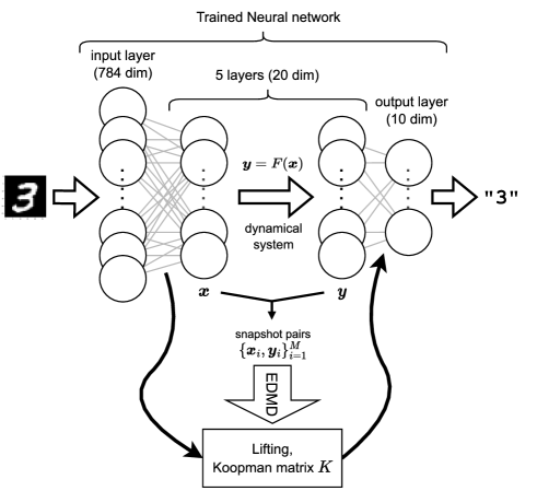
Figure 1: Neural network, dynamical system, and the partial replacement with the Koopman matrix.

3.3 Preliminary investigation of nonlinearity with the TT format

Before considering model compression, we investigate the roles of nonlinearity in the trained neural network, that is, to what extent the neural network partially replaced by the Koopman matrix replicates the original behavior of the intermediate layers.

We consider the following monomial dictionary:

$$\phi:\bm{x}\mapsto\prod_{d=1}^{D}x_{d}^{n_{d}},$$ (11)

where $0\leq n_{d}\leq N_{\mathrm{max}}$ for $d=1,2,\dots,D$. The intermediate layers in the neural network in figure 1 has $20$ nodes. Hence, even when $N_{\mathrm{max}}=2$, the dictionary size is $L=3^{20}=3,486,784,401$. We obviously cannot create the Koopman matrix with this dictionary size. Hence, the TT format is employed. We here give only a brief review of the TT format; see, for example, [22, 23, 24] for the details of the TT format.

The TT format for a tensor $\mathbf{T}\in\mathbb{R}^{n_{1}\times\cdots\times n_{D}}$ is expressed as

$$\mathbf{T}=\sum_{k_{0}=1}^{r_{0}}\cdots\sum_{k_{D}=1}^{r_{D}}\mathbf{T}_{k_{0},:,k_{1}}^{(1)}\otimes\cdots\otimes\mathbf{T}_{k_{D-1},:,k_{D}}^{(D)},$$ (12)

where $r_{0},\dots,r_{D}$ are called TT ranks, and $r_{0}=r_{D}=1$. The tensors of order $3$, $\mathbf{T}^{(d)}\in\mathbb{R}^{r_{d-1}\times n_{d}\times r_{d}}$, are called TT cores. The following formal expression for the TT core would be helpful for understanding. That is, imagine a matrix whose element is a vector as follows:

$$\left[\mathbf{T}^{(d)}\right]=\left[\begin{array}[]{ccc}\mathbf{T}_{1,:,1}^{(d)}&\dots&\mathbf{T}_{1,:,r_{d}}^{(d)}\\ \vdots&\ddots&\vdots\\ \mathbf{T}_{r_{d-1},:,1}^{(d)}&\dots&\mathbf{T}_{r_{d-1},:,r_{d}}^{(d)}\end{array}\right],$$ (16)

where $\mathbf{T}_{i,:,j}^{(d)}$ means the vector.

It is possible to construct the TT format for the dictionary vector $\bm{\Phi}(\bm{x}_{t})\in\mathbb{R}^{n_{1}\times\cdots\times n_{D}}$; in [27], the algorithm with higher-order CUR decomposition was given. We here employ an algorithm based on the singular value decomposition, which is implemented in scikit_tt [28]. In our experiments, the rank for each singular value decomposition is truncated so that the cumulative contribution of the singular values is over 0.999. Note that we must calculate $\bm{\Phi}(X)^{\dagger}$, i.e., not only a data point $\bm{x}_{t}$ but for the data matrix $X$. Hence, adding a core indicating the data number, we compress $\bm{\Phi}(X)\in\mathbb{R}^{n_{1}\times\cdots\times n_{D}\times n_{D+1}}$ in the TT format, where $n_{D+1}\in\{1,2,\dots,M\}$. The TT format of $\bm{\Phi}(Y)$ is calculated in the same way.

It is not enough to calculate $\bm{\Phi}(X)^{\dagger}$ and $\bm{\Phi}(Y)$ since our final aim is to obtain the Koopman matrix $K^{\top}=\bm{\Phi}(Y)\bm{\Phi}(X)^{\dagger}$ and to predict $\bm{y}_{t}=F(\bm{x}_{t})$ from $\bm{x}_{t}$. Although the TT format for the Koopman matrix is obtained in [26], the prediction step needs some techniques even for the TT format to reduce the memory size; we explain them in Appendix A.

Here, we use $M=10,000$ snapshots to construct the Koopman matrix $K$. We perform numerical experiments by changing the maximum degree $N_{\mathrm{max}}$ in the dictionary to $1,2,3$ and $4$. Since the number of variables is $D=20$, the dictionary size for $N_{\mathrm{max}}=4$ is $5^{20}\simeq 9.5\times 10^{13}$ for the naive construction. Hence, the number of elements of Koopman matrix becomes $5^{40}\simeq 9.1\times 10^{27}$, which memory size is about $7.2\times 10^{19}$ GB for double-precision floating-point format. By contrast, in the TT format, the final memory size for the Koopman matrix was about $1.5$ GB.

Figure 2: Prediction errors for $100$ test points. Error bars correspond to the standard deviation for $5$ different experiments. The horizontal axis is the maximum degree for each variable, $N_{\mathrm{max}}$, in the dictionary.

After constructing the Koopman matrix, we take $100$ test data and evaluate the prediction errors. Repeating the whole steps with $5$ different random seeds, the standard deviation for the prediction errors in the sense of the $L_{2}$ norm is evaluated. Figure 2 gives the numerical results, in which the error bar means the standard errors for the $5$ repeated experiments. From figure 2, we see that the setting with $N_{\mathrm{max}}=3$ roughly yields enough predictions. These results suggest that higher-order nonlinearity is not necessary for the neural network for this classification problem. Of course, the dictionary includes higher order functions as monomials; for example, the term $x_{1}^{2}x_{2}^{2}\dots x_{20}^{2}$ is included for the case with $N_{\mathrm{max}}=2$. However, one would expect that restricted nonlinearity could be enough for constructing the neural network for this problem. We will discuss this point below.

From these preliminary numerical experiments with the TT format, we expect the possibility of compression of neural networks with the Koopman operator.

3.4 Practical dictionary for model compression

Although the TT format is a powerful tool for high-dimensional systems, it is still difficult to apply it naively for the learning process such as fine-tuning. In our naive code, a prediction per data takes about $0.7$ seconds for the TT format with $N_{\mathrm{max}}=3$. The TT format tells us that the limited nonlinearity could be enough. Hence, we use the more limited dictionary in the following discussion.

For numerical experiments without the TT format, we consider two cases of dictionary functions for the EDMD algorithm. One is the monomial dictionary $\{\phi:\bm{x}\mapsto\prod_{i=1}^{D}x_{i}^{n_{i}}\mid 0\leq\sum_{i=1}^{D}n_{i}\leq N_{\max}^{\mathrm{total}}\}$, specified with a constant $N_{\mathrm{max}}^{\mathrm{total}}$. Note that $N_{\mathrm{max}}^{\mathrm{total}}$ is different from $N_{\mathrm{max}}$ in the TT format; $N_{\mathrm{max}}^{\mathrm{total}}$ is the maximum of the total degrees of the monomial exponents for each variable. For example, the dictionary here does not have $x_{1}^{2}x_{2}^{2}$ for $N_{\max}^{\mathrm{total}}=3$ since the total degree of this term is $4$.

In addition to the simple monomial dictionary, we use the Gaussian radial basis function (RBF) dictionary (including identity mapping) as the second case. The center point $\bm{c}$ of the Gaussian RBF $\phi(\bm{x})=\exp(-\varepsilon\|\bm{x}-\bm{c}\|^{2})$ is randomly chosen from the input of one of the snapshot pairs. The parameter $\varepsilon$ is set to $0.001$.

Table 2: Accuracy of networks in which the intermediate layers are replaced by the corresponding time evolution process with Koopman matrices.

Dictionary	Number of dictionary functions	Accuracy
Monomials up to 1st order	21	79.71%
Monomials up to 2nd order	231	93.54%
RBF	231	94.69%
Monomials up to 3rd order	1771	95.67%
RBF	1771	96.01%
Original trained neural network		95.62%

Table 3: Prediction errors of the time evolution of the state variables by the Koopman matrices.

Dictionary	Number of dictionary functions	Error
Monomials up to 1st order	21	6.6181
Monomials up to 2nd order	231	3.2294
RBF	231	2.3843
Monomials up to 3rd order	1771	2.0043
RBF	1771	1.3154

After learning neural networks, we extract a data set for which the trained network successfully recognizes the image for the MNIST data. The number of data is $58,052$. Then, we construct the Koopman matrix using these data. After that preparation, we choose $10,000$ data pairs from the MNIST test data set, and snapshot pairs are generated from the intermediate layers. We finally evaluate the performance of the constructed Koopman matrix for this test data set. Table 2 shows the classification accuracy for the test data with the networks substituted with the Koopman matrices for the intermediate layer. From table 2, we see that the classification problem can be solved with moderate accuracy even when the intermediate layer is replaced by time evolution using the Koopman matrix; the accuracy increases as the number of dictionary functions increases.

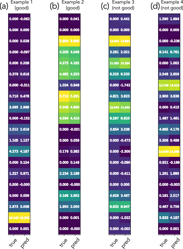
Figure 3: Examples of prediction for the intermediate layers. In each example, the left column shows the state variable after true time evolution, and the right column shows the prediction by the Koopman matrix. (a) and (b) corresponds to cases with successful prediction, and (c) and (d) are not-so-good ones.

Next, we consider the reproducibility of snapshot pairs obtained by inputting test data to the original trained neural network. Table 3 shows the average prediction errors; the prediction accuracy of the internal time evolution improves as the number of dictionary functions is increased, as does the accuracy of the classification. We also see that the simple dictionary construction here yields not so worse prediction errors compared with the TT format.

Note that the prediction at the intermediate layer is not always good when we obtain a correct result in the classification task. Figure 3 shows four examples of prediction of state variables. Although all four cases yield correct answers in the final output of the recognition task, the cases in figures 3(a) and 3(b) show good predictions in the snapshot pair prediction stage; by contrast, several predicted elements differ from the true values in figures 3(c) and (d). Why is such a ‘rough’ prediction enough for the classification problem? The reason is that only the maximum output in the network is taken as the final recognition stage. Hence, even if the prediction of the internal time evolution is not so accurate to some extent, the accuracy of the classification may not be affected.

Figure 4: Discrimination accuracy of the test data (top) and prediction error of the time evolution of the internal state variables (bottom) as the number of dictionary functions is increased.

To confirm this in more detail, we investigate the classification accuracy of the network and the prediction error of the internal time evolution when the number of RBF dictionary functions gradually increased. Figure 4 shows the results; the classification accuracy of the network reached a plateau, while the prediction errors of the internal time evolution did not fully decrease. Therefore, as discussed above, there are cases in which the classification accuracy can be maintained even if there is a certain amount of prediction errors in the time evolution. This fact suggests that model compression could be possible by approximating the internal time evolution of the neural network.

4 Numerical experiments for model compression

In this section, we perform model compression on a neural network by the proposed method. Its performance is compared with that of pruning, one of the existing model compression methods.

4.1 Experimental details

4.1.1 Model compression by the proposed method

Model compression with the proposed method is performed on the same neural network in section 3. We here use the Gaussian RBF (and identity mapping) dictionary, which makes it easier to adjust the number of dictionary functions than the monomial dictionary. Parameters and selection of center points for the Gaussian RBF are the same as in section 3.

It is possible to adjust the degree of the model compression of the proposed method by changing the number of ranks of the low-rank approximation and that of dictionary functions. As denoted in section 3.1, the low-rank approximation is performed by the singular value decomposition:

$$A=KB\simeq U\Sigma V^{\top},$$ (17)

where $U\in\mathbb{R}^{L\times L}$, $\Sigma\in\mathbb{R}^{L\times D}$, and $V\in\mathbb{R}^{D\times D}$. Note that the dimension of variables $D=20$ in the whole experiments. We select only $s$ values from the singular values $\sigma_{1},\ldots,\sigma_{s}>0\ (s\leq\min\{L,D\})$. Hence, a lower number of ranks $s$ means a highly compressed matrix.

If the number of ranks $s$ of the low-rank approximation is too large, the total number of the matrix elements in the three matrices of the singular value decomposition will increase more than that of the original matrix. Therefore, we experiment on the case without the low-rank approximation and the case with a sufficiently small number of ranks. The number of dictionary functions $L$ was tested in each case from $21$ to $120$.

4.1.2 Model compression by existing methods

For comparison, we use the conventional pruning method. Although the neural network is the same as in section 3, it is compressed by the pruning, as follows. Pruning is a method of reducing parameters by selecting unimportant weights and removing them. There are mainly two types of pruning: unstructured pruning and structured pruning. Unstructured pruning only sets some weights to 0, which does not reduce the memory used by the network to perform inference, but it is likely to have high accuracy. By contrast, in structured pruning, weights are removed in units of rows, columns, channels, and so on. Hence, we can reduce the size of the network structure and the memory size required to run the inference while it gives less accuracy than unstructured pruning.

In this experiment, we test both unstructured pruning and structured pruning and compare with the proposed method. There are several criteria for selecting the unnecessary weights. Here, we adopt magnitude-based pruning, in which the weights with the small $L_{1}$ norms are removed.

4.1.3 Comparison of performance after fine tuning

Additional training after the model compression of a network is called fine-tuning. Fine-tuning is useful when a certain amount of computational resources are available for training. Even if a significant number of parameters are reduced by model compression, we can recover the accuracy close to the uncompressed one.

Hence, we compare the performance of the proposed method with the fine-tuned conventional methods. The training procedure is the same as the first training. Only the difference is the number of epochs; the number is 5 in the fine-tuning and 14 in the original training. In the following experiments, we do not consider the center point $\bm{c}$ and the parameter $\varepsilon$ for a Gaussian RBF as training parameters.

4.2 Experimental results

4.2.1 Before fine-tuning

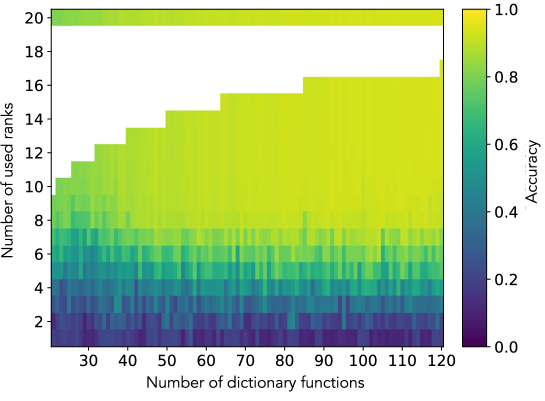
Figure 5: Accuracy of the compressed model by the proposed method for various settings. In the blank region, the number of matrix elements is greater than that of the case without singular value decomposition.

Figure 6: Number of singular values (vertical axis) at the point when the cumulative contribution of the singular values exceeds 99%. The horizontal axis is the number of dictionary functions.

Figure 5 shows the accuracy of test data of the neural network with model compression in each setting: the number of dictionary functions and the number of ranks, which are shown in the vertical and horizontal axes, respectively. Note that we plot the results without singular value decomposition for the uppermost part of figure 5. When the number of ranks is 20, which equals the dimension of the state variable, the singular value decomposition only increases the number of matrix elements and does not change the calculation results. Hence, the results without performing singular value decomposition are shown. The blank space corresponds to the region where the total number of matrix elements in the three matrices of the singular value decomposition are greater than that of the case without singular value decomposition.

From figure 5, we see that the accuracy increases gradually as the number of dictionary functions increases. Note that we achieve roughly the same accuracy in the region where the ranks are greater than 10 regardless of the number of dictionary functions. We plot the number of singular values with which the cumulative contribution of singular values exceeds 99% in figure 6. These results indicate that about 10 singular values are enough to approximate the behavior of the intermediate layer.

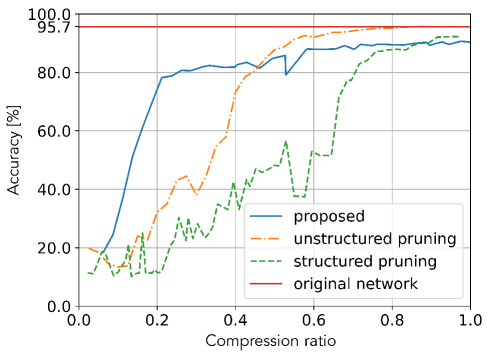
Figure 7: Accuracy for various compressed models against compression ratio which is proportional to the number of parameters in the intermediate layer of the network.

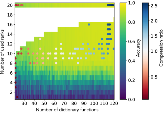
Figure 8: Accuracy on the validation data and the settings adopted for each compression ratio.

Figure 7 shows the accuracy of the test data for various compression ratios. The vertical axis represents the accuracy, and the horizontal axis represents the compression ratio. In this work, we define the compression ratio as the ratio of the number of parameters in the intermediate layer of the network after compression to those of the original network. Hence, the smaller compression ratio means a higher compressed network. Note that the parameters of the network compressed by the proposed method include the elements of the Koopman matrix and the variables needed to represent the center points of Gaussian RBFs used as dictionary functions. The compression ratio is evaluated with the number of the whole parameters.

To plot the accuracy of the proposed method for each compression ratio in figure 7, we determine the number of dictionary functions and ranks in the following procedure. First, the training data is split: 20% as validation data and the rest used to compress the network under various settings. Second, we seek the most accurate setting on the validation data among those with the same compression ratio. Figure 8 shows the accuracy of the proposed method on the validation data with the scatter plots corresponding to the best settings for various compression ratios. The accuracy values on these points in the scatter plots were used to plot figure 7.

When the number of parameters in the network is less than half of those in the original network, the intermediate layer replaced by the Koopman matrix results in higher accuracy than the two conventional compression methods. Indeed, figure 7 shows that the accuracy of the proposed method reaches about 80% in the range of a compression ratio of $0.2$ to $0.4$. This fact means the restricted nonlinearity replaces the intermediate layer of the network well. Actually, Figure 8 supports this fact. There are two types of scatter plots for cases with compression ratios roughly ranging from $0.2$ to $0.4$:

1. The number of dictionary functions is small, while the rank is 20; see the left-upper region in figure 8.

2. The rank is around $10$, while the number of dictionary functions is not so small; see the light green region in figure 8.

Hence, a small number of substantial dictionary functions is enough to mimic the intermediate layer.

Then, we conclude that the proposed compression method with the Koopman matrix works well.

4.2.2 After fine-tuning

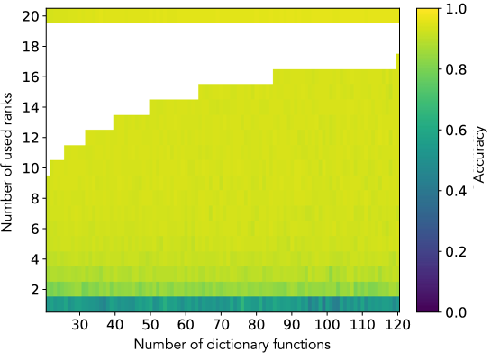
Figure 9: Accuracy of fine-tuned compressed model by the proposed method.

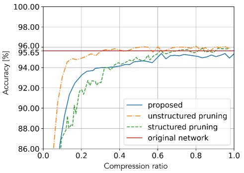
Figure 10: Comparison of accuracy for various compressed models after fine-tuning.

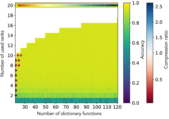
Figure 11: Accuracy on the validation data after fine-tuning and the best settings adopted for each compression ratio.

Next, we show the experimental results for the case of fine-tuning. Figure 9 shows the accuracy of the fine-tuned compressed model by the proposed method. Figure 10 plots the accuracy versus compression ratio for the proposed and the conventional methods. Figure 11 shows the accuracy of the validation data after fine-tuning and the best settings adopted for each compression ratio, as in figure 8.

Compared with figure 5, we see clear improvements in accuracy in figure 9; the fine-tuning works well. Note that figure 10 means that the fine-tuning considerably improves the accuracy of the conventional two methods. The proposed method yields a similar accuracy with the structured pruning for region of the compression ratio smaller than $0.4$. However, the accuracy of the proposed method is lower than those of the two conventional methods, especially for the compression ratio larger than $0.4$. We understand the reason from figure 11. That is, most of the best settings are obtained when the rank is $20$, which means no effects of the singular value decomposition. These results suggest that the structure of the Koopman matrix after singular value decomposition could not be suitable for fine-tuning.

Considering that the proposed method reduces the structure of the network itself and reduces the runtime memory as well as structured pruning, we conclude that the performance of the proposed method is comparable to that of the conventional method when the degree of compression is high.

5 Conclusion

In this study, we proposed a new model compression method for neural networks by applying Koopman operator theory. We performed model compression on a network for recognition tasks of the handwritten numbers. The experimental results showed that the performance of the proposed method is comparable to that of the conventional method when the models are highly compressed. Note that the proposed method removes the activation function in the intermediate layers; only the Koopman matrix acts on the intermediate process. Even in this simple replacement, the network works well.

There is room for further study in the case of other network structures and different compression methods of matrices. In addition to model compression, we expect the Koopman operator to extract useful information from neural networks. Our approach is based on the theory of dynamical systems, and there are many studies on this topic. We must tackle high-dimensional problems that stem from large neural networks. We believe that the Koopman operator theory and the TT format used in this work could help future works that provide insights into the internal mechanisms of black-box neural networks.

Appendix A Construction and usage of Koopman matrix in the TT format

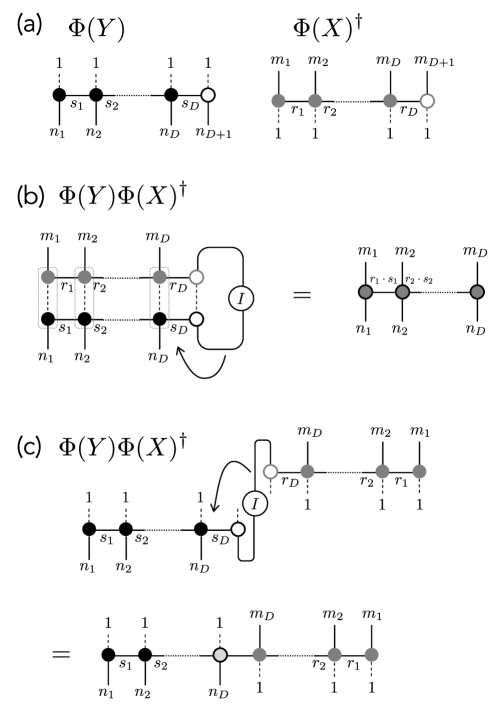
Figure 12: Two ways of the construction of Koopman matrix in the TT format. (a) shows the TT formats for $\bm{\Phi}(Y)$ and $\bm{\Phi}(X)^{\dagger}$. (b) is the naive construction of the Koopman matrix, whose TT cores are constructed by matrices, not vectors. (c) is another construction of the Koopman matrix, in which vectors are elements of the TT cores.

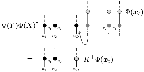
Figure 13: TT format for the prediction. We finally obtain $K^{\top}\bm{\Phi}(\bm{x}_{t})=\bm{\Phi}(Y)\bm{\Phi}(X)^{\dagger}\bm{\Phi}(\bm{x}_{t})$.

In [26], the Koopman matrix is constructed with the TT format; the constructed Koopman matrix is compared to exact solutions. For our purpose, we need to make predictions for the snapshot pairs. We need some simple techniques for this purpose; here we yield them with the diagram notations.

The Koopman matrix is a kind of operator. As denoted in section 3, the TT formats for $\bm{\Phi}(Y)$ and $\bm{\Phi}(X)^{\dagger}$ are constructed from data. Figure 12(a) shows these TT formats. Here, we also depict the dashed line with $1$, which means that a column vector in the TT core is considered as a $N_{\max}\times 1$ matrix, not a vector. Actually, the implementation in scikit_tt [28] obeys this interpretation of the TT cores. Then, a naive construction of the Koopman matrix should be the form in figure 12(b). Note that the ranks are given as the multiplications of ranks of $\bm{\Phi}(Y)$ and $\bm{\Phi}(X)^{\dagger}$. In our numerical experiments with the number of data $M=10,000$, the final ranks become the order of thousands, and it is not tractable even in the TT format.

Hence, we use the different contraction for the two TT formats for $\bm{\Phi}(Y)$ and $\bm{\Phi}(X)^{\dagger}$, as depicted in figure 12(c). Clearly, the elements of TT cores is not usual matrices but vectors. However, we can avoid the multiplicative increase of the ranks, and the prediction is also possible as depicted in figure 13. Numerical results in section 3.3 were obtained with this techniques of the TT format for the Koopman operator.

References

- [1] Liang T, Glossner J, Wang L, Shi S, and Zhang X 2021 Neurocomputing 461 370.
- [2] Gale T, Zaharia M, Young C, and Erich Elsen E 2020 In Proc. Int. Conf. High Performance Computing, Networking, Storage and Analysis p 17
- [3] Tai C, Xiao T, Zhang Y, Wang X, and E W 2016 In Proc. 4th International Conference on Learning Representations (available at: http://arxiv.org/abs/1511.06067)
- [4] Kim Y D, Park E, Yoo S, Choi T, Yang L, and Shin D 2016 In Proc. 4th International Conference on Learning Representations (available at: http://arxiv.org/abs/1511.06530)
- [5] Aggarwal V, Wang W, Eriksson B, Sun Y, and Wang W 2018 In Proc. 2018 IEEE/CVF Conf. Comp. Vision and Pattern Recognition p 9329
- [6] Koopman B O. 1931 Proc. Nat. Acad. Sci. 17 315
- [7] Rowley C, Mezić I, Bagheri P, Schlatter S, and Henningson D 2009 J. Fluid Mech. 641 115
- [8] Williams M O, Kevrekidis I G, and Rowley C W 2015 J. Nonlinear Sci. 25 1307
- [9] Mauroy A and Gonçalves J M 2020 IEEE Tran. Auto. Control 65 2550
- [10] Korda M and Mezić I 2018 Automatica 93 149
- [11] Brunton S L, Budišić M, Kaiser E, and Kutz J N 2022 SIAM Rev. 64 229
- [12] Li Q, Dietrich F, Bollt E M, and Kevrekidis I G 2017 Chaos 27 103111
- [13] Takeishi N, Kawahara Y, and Yairi T 2017 In Proc. 31st Int. Conf. Neural Information Processing Systems p 1130
- [14] Lusch B, Kutz J N, and Brunton S L 2018 Nature Comm. 9 4950
- [15] Azencot O, Erichson N B, Lin V, and Mahoney M 2020 In Proc. 37th Int. Conf. Machine Learning 119 475
- [16] Dogra A S and Redman W 2020 Advances in Neural Information Processing Systems 33 2087
- [17] Redman W T, Fonoberova M, Mohr R, Kevrekidis Y, and Mezić I 2022 In Int. Conf. Learning Representations (available at: https://openreview.net/forum?id=pWBNOgdeURp)
- [18] Konishi T and Kawahara Y 2023 Neural Networks 165 393
- [19] Lu Y, Zhong A, Li Q, and Dong B 2018 In Proc. 35th Int. Conf. Machine Learning 80 3276
- [20] Chen R T Q, Rubanova Y, Bettencourt J, and Duvenaud D K 2018 Advances in Neural Information Processing Systems 31 6571
- [21] Chang B, Chen M, Haber E, and Chi E H 2019 In Proc. Int. Conf. Learning Representations (available at: https://openreview.net/forum?id=ryxepo0cFX)
- [22] Oseledets I V 2009 Doklady Math. 80 495
- [23] Oseledets I V and Tyrtyshnikov E E 2009 SIAM J. Sci. Comput. 31 3744
- [24] Oseledets I V 2011 SIAM J. Sci. Comput. 33 2295
- [25] Klus S, Gelß P, Peitz S, and Schütte C 2018, Nonlinearity 31 3359
- [26] Gelß P, Klus S, Eisert J and Schütte C 2019 J. Comput. Nonlinear Dyn. 14 061006
- [27] Nüske F, Gelß P, Klus S, and Clementi C 2021 Physica D 427 133018
-
[28]
scikit_tt(available at: https://github.com/PGelss/scikit_tt)