Identifying circular orders for blobs in phylogenetic networks

Abstract

Interest in the inference of evolutionary networks relating species or populations has grown with the increasing recognition of the importance of hybridization, gene flow and admixture, and the availability of large-scale genomic data. However, what network features may be validly inferred from various data types under different models remains poorly understood. Previous work has largely focused on level-1 networks, in which reticulation events are well separated, and on a general network’s tree of blobs, the tree obtained by contracting every blob to a node. An open question is the identifiability of the topology of a blob of unknown level. We consider the identifiability of the circular order in which subnetworks attach to a blob, first proving that this order is well-defined for outer-labeled planar blobs. For this class of blobs, we show that the circular order information from 4-taxon subnetworks identifies the full circular order of the blob. Similarly, the circular order from 3-taxon rooted subnetworks identifies the full circular order of a rooted blob. We then show that subnetwork circular information is identifiable from certain data types and evolutionary models. This provides a general positive result for high-level networks, on the identifiability of the ordering in which taxon blocks attach to blobs in outer-labeled planar networks. Finally, we give examples of blobs with different internal structures which cannot be distinguished under many models and data types.

[1] organization=Department of Mathematics and Statistics, University of Alaska - Fairbanks, postcode=99775-6660, state=AK, country=USA [2] organization=Department of Mathematics, California State University, San Bernardino, postcode=92407, state=CA, country=USA [3] organization=Department of Statistics, University of Wisconsin - Madison, postcode=53706, state=WI, country=USA [4] organization=Department of Botany, University of Wisconsin - Madison, postcode=53706, state=WI, country=USA

1 Introduction

The statistical inference of evolutionary relationships between taxa is a substantial challenge for phylogenetic methods when both incomplete lineage sorting and hybridization (or events such as introgression, admixture or gene flow) have occurred. Many basic questions remain about what features of a network it is even possible to infer in a statistically consistent manner, under the Network Multispecies Coalescent (NMSC) as well as simpler stochastic models. The theoretical precursor of this question is that of parameter identifiability: from the distribution of some data type under some generative model, what parameters, or functions of parameters can be determined?

While progress has been made in recent years, much of this has been in the setting of level-1 networks, where the cycles in species networks caused by hybridizations are disjoint [22, 9, 17, 25, 1]. Equivalently, the biconnected components, or blobs, have only 1 reticulation in level-1 networks. See also [8] for some results on the level-2 case.

In this work, we push beyond level-1, to consider the class of outer-labeled planar networks, in which the network can be drawn in the plane with no edge crossings, with the taxa lying on the “outside” of the drawing. While level-1 networks have this property, networks of higher level may also. More specifically, our analysis proceeds by analyzing individual blobs in the network, so our results apply to all blobs that are outer-labeled planar, even if other blobs in the network are not. We show that from certain summary information on the subnetworks induced by subsets of 4 taxa, we can determine a unique circular order of taxon blocks around each such blob, which might be considered its “outer” structure. Combined with recent results on inferring the tree of blobs of a network, this determines information about planar embeddings of the network. Although we do not obtain results on the more detailed “inner” structure of the blobs, we believe this is the first detailed general result on identifiability of network’s blob topologies beyond the level-1 case.

Our starting point for this combinatorial result is the following information. First, we assume the unrooted reduced tree of blobs of the network is known. Recent work has established that this is identifiable from pairwise average distances along the species network [25] for a non-coalescent model and, under the NMSC model with generic numerical parameters, from quartet concordance factors [2]. In the course of our work here, we obtain a similar result on identifiability from logDet distances between genomic sequences, for ultrametric networks.

Second, we assume that for each choice of 4 taxa from distinct blocks “around” the blob we know that the induced 4-taxon network has either a 4-blob with a known circular order of the 4 taxa, or instead has an edge that, when removed, disconnects the 4 taxa into two known groups of 2 taxa.

To connect this identifiability result to data, we consider several data types that have been studied or used for practical network inference. These are average genetic distances [25], quartet concordance factors [22, 9, 4], and genomic logDet distances [3] for ultrametric networks. For each, we give identifiability results for outer-labeled planar networks under several statistical models of gene tree and sequence evolution. Gene tree models range from the simplest “displayed tree” model, to a coalescent model on displayed trees, to the full coalescent model on a network in which lineages behave independently. Sequence evolution models are those commonly adopted in phylogenetics, although some analyses make further assumptions such as constant mutation rates, or restrictions on edge lengths in blobs.

Finally, for several of these data types we construct new examples of networks whose structures are not fully identifiable. These include blobs which may be large (involving more than 4 taxon blocks) and of high level (involving more than one hybridization). While the existence of such examples is a negative result, the examples are an important contribution to understanding the limits of which network topological features may be identifiable, which is vital to advancing practical inference.

2 Phylogenetic networks and blobs

2.1 Networks

We adopt the definitions concerning networks from [6], but introduce terminology informally here.

A rooted topological phylogenetic network $N^{+}$ on a set of taxa $X$ is the basic object of interest. Such a network is a rooted directed acyclic graph (DAG). We require the leaves to be of degree 1. An edge incident to a leaf is called pendent. The edges of $N^{+}$ are partitioned into hybrid edges which share child nodes with at least one other partner hybrid edge, and tree edges which do not share child nodes. Its nodes are either the root, hybrid nodes which are children of hybrid edges, or tree nodes. A network is binary if the root has degree 2 and all other internal nodes have degree 3. The leaves of $N^{+}$ are bijectively labeled by elements of $X$.

A network $N^{+}$ may be given a metric structure by assigning to each edge $e$ a pair of parameters $(\ell(e),\gamma(e))$, where $\ell(e)\geq 0$ is an edge length with $\ell(e)>0$ for tree edges, and $\gamma(e)\in(0,1]$ is a hybridization or inheritance parameter which sums to 1 over all partner edges with a common child node. For any tree edge $e$ this means $\gamma(e)=1$. Although it is sometimes desirable to allow pendent edges to have 0 length, e.g. to include multiple individuals from the same population, or extinct taxa ancestral to extant taxa, for simplicity we rule that out. Nonetheless our results generalize to that situation with straightforward adjustments.

We say a node or edge is ancestral to or above another in $N^{+}$ if there is a, possibly empty, directed path from the first to the second.

The least stable ancestor (LSA) of the taxa on a network $N^{+}$ is the lowest node through which all directed paths from the root to any taxon must pass. Under standard models, most sources of data, as well as the quartet information we assume we can access in Section 6, give no information about the structure of $N^{+}$ above the LSA. We therefore consider the LSA network induced by $N^{+}$, as obtained by deleting all edges and nodes strictly ancestral to the LSA, and rerooting at the LSA. We make the following assumption for the remainder of this work.

Assumption 1.

The network $N^{+}$ has no edges above its LSA, that is, its LSA is its root.

For a network $N^{+}$ on $X$, a network $N^{+}_{1}$ on $X_{1}\subseteq X$ is displayed in $N^{+}$ if it can be embedded in $N^{+}$ with a label-preserving map such that edges of $N^{+}_{1}$ map to edge-disjoint directed paths in $N^{+}$ (see [6] for more details). In particular, a tree $T^{+}$ on $X$ is displayed in $N^{+}$ if it can be obtained by deleting all but one parent edge from each hybrid node in $N^{+}$, along with remaining edges no longer on up-down paths between taxa, and additional edges and nodes so $T^{+}$ satisfies 1. We generally do not suppress degree-2 nodes so each edge in $T^{+}$ maps to a single edge in $N^{+}$.

For a tree $T$ on $\{a,b,c,d\}$, $T$ displays the quartet $ab|cd$ if $T$ has an edge that, when removed, disconnects $T$ and partitions the leaves as $ab|cd$. A network $N^{+}$ displays $ab|cd$ if there exists a tree $T$ displayed in $N^{+}$, that displays $ab|cd$.

The semidirected network $N^{-}$ associated to $N^{+}$ is the unrooted network obtained from the LSA network induced by $N^{+}$ by undirecting all tree edges while retaining directions of hybrid edges, and suppressing the LSA if it is of degree 2. Edges and nodes in $N^{-}$ inherit classifications as hybrid or tree from those of $N^{+}$. When we refer to a semidirected network, we always assume it is obtained from a rooted phylogenetic network in this way. In particular, it is always possible to root a semidirected network, directing all non-hybrid edges away from the root consistently with the already directed hybrid edges.

The results obtained in later sections apply to both rooted and semidirected networks so we refer to a network as $N$ without superscript to reflect this generality, unless stated otherwise with more specific $N^{+}$ or $N^{-}$ notation. However, in proving results that apply to semidirected networks, it is often more efficient to work in the context of rooted networks. One of the key concepts used in our arguments, the funnel of Definition 3, is inherently a rooted notion, and can differ for different rootings of a semidirected network. Others, such as the lowest nodes of blobs of Definition 1, can be defined in semidirected networks (i.e, they are invariant to a choice of root), but are simpler to describe in a rooted setting.

2.2 Blobs

A cut node in a graph is a node whose deletion disconnects the graph. A cut edge in a graph is an edge whose deletion disconnects the graph. It is common to define blobs in networks as maximal connected subgraphs with no cut edges (i.e., as maximal 2-edge-connected subgraphs). For this work we adopt a stricter definition. A blob is a maximal subgraph with no cut nodes, that is, a maximal biconnected subgraph. A trivial blob is a blob with at most one edge, so that cut edges are considered trivial blobs.

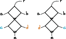
Figure 1: Two planar embeddings of a network. Under the definition of a blob adopted in this work, as a biconnected component, the central structure is composed of two blobs, whose circular orders of articulation nodes are the same in both embeddings. If blobs were defined as 2-edge-connected components, there would be only one blob but the embeddings would give different circular orders.

The differences in these definitions is illustrated in Figure 1. By our definition, using biconnectedness, the left figure shows two blobs of four edges each. Under the 2-edge-connected definition, all eight edges form a single blob. Our interest is in possible orders of taxa around planar embeddings of the graph, and the right figure shows an alternative planar embedding of the same graph. Viewed as two blobs, the orders of taxa around each blob are unchanged, but viewed as a single blob there are two distinct orders. Our results are simpler to state by adopting the biconnected definition. In general, biconnected components are subgraphs of 2-edge-connected components, so we work with a finer decomposition of a network. However, for binary networks the two notions of non-trivial blobs coincide, although trivial blobs differ (cut edges versus cut nodes).

For a binary network $N$, its tree of blobs $T$ is obtained by contracting each non-trivial blob into a single node [13, 25, 2]. Since $N$ is binary, distinct non-trivial blobs do not share any node and correspond to distinct nodes in $T$. The edges of $T$ correspond to cut edges of $N$, so $T$ is roooted if $N$ is rooted, and $T$ is unrooted if $N$ is semidirected. The reduced tree-of-blobs is obtained by suppressing any degree-2 node in $T$, other than its root if $T$ is rooted.

Since a phylogenetic network has no directed cycles, we use the term cycle to refer to a subnetwork which forms a cycle when all edges are undirected. Any cycle either is or lies in a non-trivial blob.

An articulation node of a blob $B$ in $N$ is a node in $B$ that is a leaf or incident to an edge of $N$ that is not in $B$. A blob with $m$ distinct articulation nodes is called an $m$-blob. Assumption 1 implies that if the LSA of $N$ is in a non-trivial blob, then it is not an articulation node of that blob, even though it would have been if $N$ had additional edges above the LSA.

3 Structure of general blobs

In this section, we define less standard terminology, and establish some facts about arbitrary blobs which will be useful in later sections.

A subset of nodes that will play a special role in our arguments is the following.

Definition 1.

A lowest node of a blob is a node in the blob which has no descendent nodes in the blob.

The following result characterizes a non-trivial blob’s lowest nodes, and shows that they are well-defined on a semidirected network because they are independent of the root location.

Lemma 3.1.

Let $B$ be a non-trivial blob in a rooted phylogenetic network. Then the lowest nodes of $B$ are precisely the hybrid articulation nodes of $B$ which have no descendent edges in $B$.

Proof.

Let $v$ be a lowest node of $B$. Since the network’s leaves are the only nodes with no descendent edges, and they are in trivial blobs, $v$ must have one or more descendent edges. Since $v$ is lowest, these descendent edges are not in $B$, and hence $v$ is an articulation node of $B$. If $v$ were not hybrid, then it would have exactly one parental edge, which is in $B$. But then the parent of $v$ would be a cut node of $B$, contradicting its biconnectedness.

Conversely, if $v\in B$ has no descendent edges in $B$, then $v$ is a lowest node of $B$. ∎

As an immediate consequence, if a network is binary then the lowest nodes of a non-trivial blob $\cal B$ are precisely its hybrid articulation nodes: For a binary network, any hybrid articulation node of $\cal B$ has a single descendent edge, which cannot be in $\cal B$.

We also use the notion of LSAs for blobs $B$ of a rooted network $N^{+}$, as the lowest node in $N^{+}$ through which all paths from the root to any node in $B$ must pass. While this LSA need not be in $B$, a priori, the following shows it is.

Lemma 3.2.

The LSA of a blob $B$ in a rooted phylogenetic network lies in $B$.

Proof.

A node $v$ in a blob $B$ is said to be an entry node of $B$ if there exists an edge not in $B$ with child $v$. $B$ has at most one entry node, since if two exist, picking directed paths from the network root through those nodes would allow us to contradict that $B$ is a maximal biconnected subgraph.

If $B$ has no entry nodes then the network’s root is in $B$ and is $B$’s LSA. If $B$ has only one entry node, it is the LSA of the blob. ∎

In a binary network, if a non-trivial blob’s LSA and the network’s root (assumed to be the network’s LSA) are the same, that node is not incident to an edge outside the blob, and so is not an articulation node of the blob. If the LSAs of the blob and the network differ, however, the LSA of the blob is an articulation node. For a binary network, such an LSA must be a tree node.

Definition 2.

A trek cycle (or up-down cycle) in a DAG is a pair $(L,R)$ of directed paths from a node $w$ (the source) to a node $v$ (the sink), with no nodes other than $w$ and $v$ in common.

A trek cycle $(L,R)$ forms a cycle in the usual sense by concatenating the reversal of $L$ with $R$. In a phylogenetic network the sink node in a trek cycle must be hybrid.

The following, Lemma 10 of [6], identifies useful substructures in blobs, to simplify later arguments.

Lemma 3.3.

For a non-trivial blob $B$ in a DAG, every edge or node in $B$ is contained in a trek cycle within $B$. Thus $B$ is a union of (non-disjoint) trek cycles.

Although the proof of the following is trivial, we state it for use in later arguments.

Lemma 3.4.

Every node in a blob $B$ in a rooted phylogenetic network is ancestral to at least one lowest node of $B$.

This lemma implies that every blob has at least one lowest node, and hence every non-trivial blob has at least one hybrid articulation node.

Definition 3.

The funnel of a lowest node $v$ of a blob $B$ is the set of edges and nodes in $B$ that are ancestral to $v$ but not to any other lowest node of $B$.

The term “funnel” was used differently by Xu and Ané [25] for a similar concept on semidirected networks, involving only hybrid edges. The notion used here is for rooted networks, as a funnel may depend on the root position. The funnel of a lowest node may contain both tree and hybrid edges and nodes, and tree or hybrid articulation nodes, as shown in Figure 2. Furthermore, it may contain an edge without containing the parental node of that edge, so the funnel is not typically a subgraph. However, deleting a funnel from a blob does give a subgraph.

Lemma 3.5.

Suppose a blob $B$ has at least two lowest nodes. Then the deletion from $B$ of the funnel of a lowest node gives a non-empty connected graph.

Proof.

Let $v$ be the lowest node whose funnel was removed, and $B^{\prime}$ the resulting graph. The LSA $\rho$ of $B$ is in $B^{\prime}$ since it lies above all lowest nodes of $B$. Let $u\in B$ be any other node in $B^{\prime}$. Then there is a directed path $P$ from $\rho$ to $u$ in $B$. But since $u$ is ancestral to a lowest node other than $v$ and all edges in $P$ are above $u$, they are also ancestral to another lowest node. Thus all edges of $P$ are in $B^{\prime}$. ∎

If a blob has a single lowest node, then by Lemma 3.4 its funnel is the entire blob. Otherwise we can classify the blob’s lowest nodes into two types, illustrated in Figure 2.

Definition 4.

Suppose a blob $B$ has at least two lowest nodes, one of which is $v$. Then $v$ links $B$ if the deletion of the funnel of $v$ from $B$ results in a graph with two or more (possibly trivial) blobs. If a lowest node does not link $B$ (that is, the deletion of its funnel results in a single blob) we say it augments $B$.

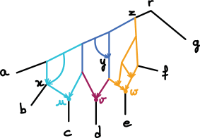
Figure 2: Network with one non-trivial blob $B$ (all colored edges) with three lowest nodes, $u$, $v$ and $w$ (colored dots). Articulation nodes that are not lowest can be tree nodes (e.g. node adjacent to $a$) or hybrid nodes (e.g. $x$, non-binary node). The funnel of each lowest node is shown with matching color. Lowest node $v$ links $B$, since deletion of its funnel from $B$ gives two blobs (with lowest nodes $u$ and $w$) joined by a cut edge. Node $w$ similarly links the blob, since deleting its funnel leaves one blob with lowest nodes $u,v$ and one trivial blob, the blue edge incident to $z$. Lowest node $u$ augments the blob, since deleting its funnel leaves a single blob. This example is planar for clarity, though planarity is not assumed in the definition of linking and augmenting lowest nodes.

Lemma 3.6.

Every blob with 2 or more lowest nodes has at least one lowest node that augments it.

Proof.

Suppose every lowest node of a blob $B$ links it. Deletion of the funnel for any lowest node $v$ leaves a connected graph by Lemma 3.5. Since the lowest nodes are linking, these graphs have one or more cut nodes. Associate to each such lowest node $v$ of $B$ one of the lowest such cut nodes $w_{v}$ resulting from the funnel deletion, and let $w_{v}$ also denote the node in $B$ that induces it. Of the set of associated cut nodes for all lowest nodes, choose a lowest one, $\tilde{w}=w_{\tilde{v}}$, with $\tilde{v}$ a lowest node of $B$ associated to $\tilde{w}$.

When the funnel of $\tilde{v}$ is deleted from $B$, the node $\tilde{w}$ becomes a cut node above one or more blobs. But since $\tilde{w}$ is the lowest such cut node, it can be above only one blob, $B^{\prime}$, to which it is incident. Since $\tilde{w}$ is not in the funnel of $\tilde{v}$, it must lie above some lowest node $u\neq\tilde{v}$ in $B$. Then $u$ must be hybrid, $B^{\prime}$ must be non-trivial and $u$ must be in $B^{\prime}$.

By Lemma 3.3, $\tilde{w}$ is in a trek cycle in $B$. Since $\tilde{w}$ becomes a cut node when the funnel of $\tilde{v}$ is removed, this trek cycle includes some edge in the funnel. But then the sink of the trek cycle must be in the funnel, and hence above $\tilde{v}$. Thus $\tilde{w}$ is above both $\tilde{v}$ and $u$.

Deleting the funnel of $u$ from $B$, then, cannot delete $\tilde{w}$ or any node in the funnel of $\tilde{v}$, and hence only deletes nodes in $B^{\prime}$. Thus deleting the funnel of $u$ from $B$ can only produce cut nodes from nodes below $\tilde{w}$. But such a cut node would be lower than $\tilde{w}$ , which is a contradiction to the choice of $\tilde{w}$ as a lowest node in the set $\{w_{v},\,v\mbox{ lowest in }\cal B\}$.

Thus $B$ has an augmenting lowest node. ∎

In the next section we will use deletion of funnels of lowest nodes in an inductive proof. The following Lemma describes the impact on the number of lowest nodes.

Lemma 3.7.

Let $B$ be a blob with $n\geq 2$ lowest nodes. Then the deletion of a funnel of any lowest node produces a graph with exactly $n-1$ lowest nodes among its blobs.

Proof.

Let $B^{\prime}$ be the subgraph of $B$ obtained by deleting the funnel of a lowest node $v$. The $n-1$ lowest nodes of $B$ other than $v$ are not in $v$’s funnel, hence are in blobs of $B^{\prime}$ and remain lowest nodes.

Suppose there is a lowest node $w$ of $B^{\prime}$ that is not a lowest node of $B$. Then all descendent edges of $w$ in $B$ are in the funnel of $v$, and hence $w$ lies above $v$ and no other lowest node of $B$. Therefore $w$ is in the funnel of $v$, and not in $B^{\prime}$. ∎

4 Circular orders and outer-labeled planar blobs

We are interested in natural orders of taxa around a phylogenetic network embedded in the Euclidean plane, so that as a plane graph, vertices are distinct and edges only meet at their end-points. Generally, networks do not have a unique order in which their taxa are arranged, since at any cut node one can “rotate” one part of the network out of the plane, reversing the order of its taxa, as was illustrated in Figure 1. However, the individual blobs of such a network are associated to a unique order, as we establish in this section. We seek an order of blocks of taxa around a blob, but first define these blocks.

Definition 5.

For a blob $B$ in a network on $X$, the taxon blocks associated with $B$ are the non-empty subsets of $X$ on connected components obtained by deleting all edges in $B$.

The taxon blocks for a blob are in bijective correspondence to the articulation nodes of the blob, according to the articulation node through which any undirected path from the blob to a taxon in the block must pass. This correspondence relies upon 1, so that the blob’s LSA is not considered an articulation node when it coincides with the network LSA.

Definition 6.

A circular order for a finite set $Y$ is an order $(y_{1},y_{2},\dots,y_{k})$ of its elements up to reversal and cyclic permutation. That is, as a circular order, $(y_{1},y_{2},\dots,y_{k-1},y_{k})$ is the same as $(y_{k},y_{k-1},\dots,y_{2},y_{1})$ and as $(y_{2},y_{3},\dots,y_{k},y_{1})$.

Viewing the articulation nodes as “labeled” by their taxon blocks, a circular order of the blocks arises from any mapping of the blob into the plane which places the labels on the “outside”. So that such an order is not completely arbitrary, we require that the mapping be an embedding. To make this precise, recall that a graph embedded in the plane divides it into connected regions called faces. Exactly one of these is an unbounded region, called the unbounded face. To simplify later wording, we adopt the following terminology.

Definition 7.

If a planar graph $G$ is embedded in the plane as $H$, the frontier of $H$ is the set of edges and nodes forming the topological boundary of the unbounded face.

The frontier of an embedded planar graph depends upon the embedding, and not just the abstract graph, as illustrated in Figure 3.

The following is a slight generalization of a definition of [18], allowing general subsets of vertices rather than the leaf set.

Definition 8.

Let $G$ be a planar graph, embedded in the plane as $H$, and $V_{0}$ a subset of the vertices of $G$. Then the embedded $H$ is outer-labeled planar for $V_{0}$ if all elements of $V_{0}$ lie in the frontier of $H$. If $G$ has any outer-labeled planar embedding for $V_{0}$, we say $G$ is outer-labeled planar for $V_{0}$. A phylogenetic network $N$ is outer-labeled planar if $N$ is outer-labeled planar for its leaf set, labeled by $X$. A blob $B$ in a phylogenetic network is outer-labeled planar if $B$ is outer-labeled planar for its set $V_{0}$ of articulation nodes, labeled by taxon blocks.

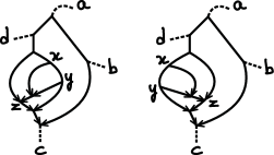
Figure 3: A planar blob $G$ may have several different outer-labeled planar embeddings. Here two such embeddings are shown for the same blob, with $V_{0}$ consisting of articulation nodes adjacent to $\{a,b,c,d\}$. On the left, hybrid node $z$ lies in the frontier but tree nodes $x$ and $y$ do not, while these are reversed on the right. However, the circular order of articulation nodes is the same for both embeddings.

If $N$ is outer-labeled planar, then each of its blobs must be, by restricting the embedding to the blob. Conversely, if all its blobs are outer-labeled planar, then the network must be, as one can construct an appropriate embedding by “gluing” those for each blob at articulation nodes.

An outer-labeled planar blob may have several different outer-labeled planar embeddings, with different sets of edges and nodes in their frontiers, as shown in Figure 3. Nonetheless, the following establishes a fundamental commonality to all such embeddings.

Theorem 4.1.

Let $G$ be an undirected biconnected graph which is outer-labeled planar for a subset $V_{0}$ of its vertices. Then the frontiers of all the planar embeddings of $G$ with $V_{0}$ in the frontier induce the same circular order of $V_{0}$.

Proof.

Let $F$ and $F^{\prime}$ denote the subgraphs of $G$ forming the frontiers of two outer-labeled planar embeddings, $H$ and $H^{\prime}$, of $G$ for $V_{0}$. Since $G$ is biconnected, by Proposition 4.2.6 of [10], $F$ and $F^{\prime}$ are cycles. Thus $F$ and $F^{\prime}$ induce circular orders $\sigma$ and $\sigma^{\prime}$ of $V_{0}$. If $|V_{0}|<4$, $\sigma=\sigma^{\prime}$ is trivial, so we henceforth assume $|V_{0}|\geq 4$.

Let $\sigma=(x_{1},x_{2},...,x_{n})$ and suppose, for the sake of contradiction, $\sigma\neq\sigma^{\prime}$. Without loss of generality, we may assume that $x_{1},x_{2}$ are adjacent in $\sigma$ but not in $\sigma^{\prime}$. Then there are four elements of $V_{0}$ with circular order $(x_{1},x_{2},x_{i},x_{j})$ induced from $\sigma$ and $(x_{1},x_{i},x_{2},x_{j})$ from $\sigma^{\prime}$.

There are two vertex-disjoint paths, $P$ and $Q$ in $F$, such that $P$ passes from $x_{1}$ to $x_{2}$ and no other node in $V_{0}$, and $Q$ passes from $x_{i}$ to $x_{j}$ and possibly other nodes in $V_{0}$ but neither $x_{1}$ nor $x_{2}$. Let $P^{\prime}_{1}$ and $P^{\prime}_{2}$ be the two distinct paths in $F^{\prime}$ going from $x_{i}$ to $x_{j}$, passing through $x_{1}$ and $x_{2}$ respectively, which are disjoint except for their endpoints, $x_{i}$ and $x_{j}$. Note that $P$ connects $P_{1}^{\prime}$ to $P_{2}^{\prime}$ and does not pass through $x_{i}$ or $x_{j}$. Let $\alpha$ be the last node on $P$ that is also on $P^{\prime}_{1}$ and $\beta$ the first node on $P$ after $\alpha$ that is on $P^{\prime}_{2}$ (see Figure 4, path in blue). Then $\alpha,\beta$ must not be in $V_{0}$ and $\alpha\neq\beta$. Let $P_{3}$ be the subpath of $P$ from $\alpha$ to $\beta$.

Consider the following 3 paths from $\alpha$ to $\beta$ that intersect only at their endpoints: the subpaths $Q^{\prime}_{1},Q^{\prime}_{2}$ of the cycle $F^{\prime}$ passing through $x_{i},x_{j}$ respectively, and the subpath $P_{3}$ of $P$ in $F$. Under the $H^{\prime}$ embedding, the path $P_{3}$ lies in the region of the plane bounded by $F^{\prime}=Q^{\prime}_{1}\cup Q^{\prime}_{2}$ (see Figure 4). Thus by Lemma 4.1.2 of [10], every path from $x_{i}$ to $x_{j}$ in $G$ must intersect $P_{3}$, in the planar embedding $H^{\prime}$. In particular, $Q$ must intersect $P_{3}$ in $H^{\prime}$. Since $H^{\prime}$ is planar, $Q$ and $P_{3}$ must intersect at a vertex, which is a contradiction since by definition they are vertex-disjoint. This contradiction yields $\sigma=\sigma^{\prime}$. ∎

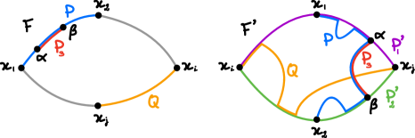
Figure 4: Schematic drawing of the paths used in the proof of Theorem 4.1 to show each outer-labeled biconnected graph $G$ induces a unique circular order on the labeled nodes. Left: frontier $F$ of an embedding $H$ of $G$. Two vertex-disjoint paths of $F$, $P$ from $x_{1}$ to $x_{2}$ (in blue), and $Q$ from $x_{i}$ to $x_{j}$ (in orange) are highlighted. Additionally, a sub-path $P_{3}$ of $P$ is shown in red. Right: frontier $F^{\prime}$ (in purple and green) of an embedding $H^{\prime}$ of $G$. Part of the frontier $F$ (paths $P$ and $Q$ in blue and orange, respectively) from the embedding $H$ is also highlighted. Between the vertices $\alpha,\beta$ are 3 paths that are disjoint except for their endpoints: two in $F^{\prime}$ and one in $F$ ($P_{3}$ in red). But then $Q$ must intersect $P_{3}$ in the plane.

Corollary 4.2.

There is a unique circular order of the articulation nodes of an outer-labeled planar blob of a phylogenetic network, induced from every outer-labeled planar embedding of the blob.

If a network $N$ on an $n$-taxon set $X$ has an $n$-blob, then each taxon block for this blob must be reduced to a single taxon, mapping each articulation node to a single taxon in $X$. Then by 6.7, all outer-labeled planar embeddings of $N$ induce the same circular order of $X$, which leads us to the following definition.

Definition 9.

Let $N$ be an outer-labeled planar network on an $n$-taxon set $X$. If $N$ has an $n$-blob, the circular order of $N$ is defined as the unique circular order of $X$ induced by all outer-labeled planar embeddings of $N$. More generally, $N$ is said to be congruent with a circular order $\sigma$ of $X$ if there exists an outer-labeled planar network $N^{\prime}$ on $X$ displaying $N$ which has an $n$-blob and circular order $\sigma$.

Note this definition differs from that defined in terms of split systems, which is used in the development of splits graphs [23, 18, 16]. Indeed, the network types differ, as ours are explicit and splits graphs are implicit. While we do not use split systems here, the following shows a connection for 4-taxon trees.

Lemma 4.3.

Let $T=ab|cd$ be a resolved 4-taxon tree. Then $T$ is congruent with exactly two circular orders: $\sigma_{c}=(a,b,c,d)$ and $\sigma_{d}=(a,b,d,c)$.

Proof.

Consider the network with a single 4-cycle, where $a$ descends from the hybrid node and, moving around the cycle $b,c,d$ are, in order, attached by edges. This network has circular order $\sigma_{c}$ and displays $T$. Interchanging the taxa $c,d$ gives a network with order $\sigma_{d}$ which also displays $T$.

To show $T$ is not congruent with $\sigma_{b}=(a,c,b,d)$ we reason similarly to the proof of Theorem 4.1. Suppose $T$ were congruent to $\sigma_{b}$, and $N$ is a 4-blob network displaying $T$ with that order. Fix an outer-labeled planar embedding of $N$, with $F$ the frontier of the blob. In the embedded $T$, let $p_{ab}$ be the unique path from $a$ to $b$ (considered undirected), and $p_{cd}$ the unique path from $c$ to $d$. Since the order along $F$ is $\sigma_{b}$, paths from $a$ and $b$ meet $F$ on different segments between the articulation nodes for $c$ and $d$: let $F_{a}$ be the segment for $a$ and $F_{b}$ that for $b$. Then we can find nodes $\alpha\in F_{a}$ and $\beta\in F_{b}$ along $p_{ab}$ and three disjoint paths between $\alpha$ and $\beta$: two segments, $F_{1}$ and $F_{2}$, of $F$ and a subpath, $p_{\alpha\beta}$, of $p_{ab}$ that intersects $F$ only at $\alpha,\beta$. Since $T=ab|cd$, $p_{ab}$ and $p_{cd}$ do not intersect, so $\alpha$ and $\beta$ must be distinct from the articulation nodes for $c$ and $d$. Since $p_{\alpha\beta}$ lies in the region of the plane bounded by $F_{1}$ and $F_{2}$, every path in $N$ between $c$ and $d$ must intersect $p_{\alpha\beta}$ by [10, Lemma 4.1.2], a contradiction since $p_{ab}$ and $p_{cd}$ do not intersect. Therefore $T$ is not congruent with $\sigma_{b}$. ∎

5 Circular orders from quartets

Having established that an outer-labeled planar blob in a phylogenetic network has a unique circular order of its articulation nodes, we turn to the question of whether this circular order can be determined from information on the network’s induced quartet networks. A positive answer will provide a pathway for showing that the circular order can be consistently inferred from certain approaches to empirical data analysis.

The following notion is similar to that of a 4-taxon set that defines an edge in a tree, which is used in the definition of a dense set of quartets for a tree [14].

Definition 10.

For a blob $B$ in a phylogenetic network, a 4-taxon set is $B$-informative if its elements are in distinct taxon blocks associated to $B$. A collection of 4-taxon sets is a full $B$-informative collection if, for each choice of 4 blocks associated to $B$, one of the 4-taxon sets contains a taxon from each block.

Given a $B$-informative 4-taxon set, it is easy to see that modulo 2-blobs the topology of the induced quartet network is dependent only on the blocks of the taxa and not the individual taxa themselves. In particular, whether such an induced network displays a 4-blob or has a cut edge separating the taxa into sets of two taxa depends only on the blocks.

The simplest example of the connection between blob structure and circular order for a 4-taxon network, is captured by the following.

Lemma 5.1.

Let $N$ be a binary network on $\{a,b,c,d\}$.

1. If $N$ has a cut edge separating $a,b$ from $c,d$, it displays only the quartet $ab|cd$. If $N$ is also outer-labeled planar, it is congruent with circular orders $(a,b,c,d)$ and $(a,b,d,c)$.

2. If $N$ has a 4-blob then it displays at least 2 quartets. If the 4-blob of $N$ is also outer-labeled planar with unique circular order $(a,b,c,d)$, then $N$ displays exactly 2 quartets, $ab|cd$ and $ad|bc$.

Proof.

In the first case, the first statement is trivial since any cut edge in $N$ must be in all displayed trees. To show that $N$ is congruent with $\sigma_{c}=(a,b,c,d)$, we build a network ${N}^{\prime}$ displaying $N$, outer-labeled planar, with a 4-blob and order $\sigma_{c}$. Since an edge incident to a leaf can be directed towards the leaf, we can build ${N}^{\prime}$ from $N$ by adding a hybrid edge from the edge incident to $c$ to the edge incident to $a$. The other order is handled similarly.

Now consider the second case, with a 4-blob. By [6, Lemma 1], $N$ must display at least 2 distinct quartets. If $N$ is outer-labeled planar, by Corollary 4.2 it has a unique circular order $(a,b,c,d)$. Then by Lemma 4.3, the displayed quartets can only be $ab|cd$ and $ad|bc$. ∎

Lemma 5.1 is extended to non-binary networks in the Appendix, Lemma A.1, which includes a third case for networks having a central node whose deletion disconnects all 4 taxa. Such networks display the star tree only, and, like the 4-taxon star tree, are congruent with all 3 circular orders. These results imply the following remarkable connection.

Corollary 5.2.

Let $N$ be a 4-taxon outer-labeled planar network. $N$ is congruent with a circular order $\sigma$ if and only if all its displayed trees are congruent with $\sigma$.

We assume that we can access the following information about induced quartet networks. Some possible sources of such information are discussed in the next section.

Definition 11.

For a binary outer-labeled planar blob $B$ in a phylogenetic network and a full $B$-informative collection of 4 taxon sets, the 4-taxon circular order information is the collection of 4-taxon orders specified by the induced outer-labeled planar quartet networks for the 4-taxon sets. More specifically, this information consists of:

1. for a quartet network without a 4-blob, and hence a cut edge inducing a split $xy|zw$ of the taxa, the circular orders are $(x,y,z,w)$ and $(x,y,w,z)$.

2. for a quartet network with a 4-blob, the circular order is the unique order induced from any outer-labeled planar embedding of the quartet network.

Theorem 5.3.

Let $B$ be a binary outer-labeled planar blob in a phylogenetic network. Then 4-taxon circular order information on a full $B$-informative set of 4-taxon sets determines the unique circular order of its articulation nodes induced by all outer-labeled planar embeddings of the blob.

In the proof below, we in fact use only information from 4-taxon sets that induce a 4-blob (item 2 in Definition 11). While order information from quartet networks without 4-blobs is potentially useful for improved data analyses, it is redundant for establishing identifiability of the blob’s circular order.

Also, while our argument establishes identifiability of the circular order, it does not suggest an efficient algorithmic way of obtaining the order. We only show that the exact 4-taxon order information is compatible with no circular order than the one arising from an outer-labeled planar embedding of the full blob.

Proof of Theorem 5.3.

We proceed by induction on the number $n$ of lowest nodes of the blob.

In the base case of $n=1$, there is only one lowest node $v$. If there are fewer than 4 articulation nodes, the result is trivial. Otherwise, for any three articulation nodes $x_{1},x_{2},x_{3}$ other than $v$, the induced quartet network on taxa chosen from the taxon blocks for $v,x_{1},x_{2},x_{3}$ has a 4-blob. This is because by Lemma 3.4 all edges in the blob are ancestral to $v$, so no edges are lost in passing to the induced network. Thus by assumption we know the circular suborder of $\{v,x_{1},x_{2},x_{3}\}$ for every such set. From these it is straightforward to deduce the unique circular order on the full set of articulation nodes.

Now let $n\geq 2$ and assume the result for blobs with $n-1$ lowest nodes. Again the result is trivial unless there are at least 4 articulation nodes, so we consider only that case. By Lemma 3.6 there is at least one lowest node $v$ that augments the blob. Let $B^{\prime}$ be the subgraph of $B$ obtained by deleting the funnel of $v$, so $B^{\prime}$ is a blob on the induced network $N^{\prime}$ on all non-descendents of $v$’s funnel edges. By Lemma 3.7. $B^{\prime}$ has exactly $n-1$ lowest nodes, all inherited from $B$. Thus a unique circular order of the articulation nodes of $B^{\prime}$ is determined by induction.

We now must show the articulation nodes of $B$ on the funnel of $v$ can be uniquely placed to extend the order for $B^{\prime}$. (Note however that we do not know which node is $v$, nor which articulation nodes lie on $B^{\prime}$ or the funnel of $v$; we simply have a full $B$-informative collection of sets of 4 taxa which determines the unique circular order on some subset of the articulation nodes of $B$ which includes all those on the unknown $B^{\prime}$, and we want to show that we have enough information to extend the circular order to the full set of articulation nodes.)

We consider two cases:

If $B^{\prime}$ has only one lowest node, $u$, then taxa from the blocks for $u,v$ and any two other articulation nodes $x,y$ of $B$ induce a quartet network with a 4-blob. This is because every edge in $B$ must be ancestral to $u$ or $v$ by Lemma 3.4, so passing to an induced quartet network on taxa in the blocks for these four articulation nodes retains all edges in the blob, and thus produces no cut nodes from the blob. Since we have circular orders for each such choice of taxa, varying $x,y$ is enough to determine a full circular order for the blob. Note that in this case we did not need to use the already-determined circular order on $B^{\prime}$.

If $B^{\prime}$ has at least 2 lowest nodes, we consider two subcases depending on the location of $v$ in the frontier of the embedded blob. In the first, $v$ is between neighboring lowest nodes $u,w$, with the LSA of the blob $L$ not between $u$ and $v$ or between $v$ and $w$. In the second $L$ is an articulation node, there are no lowest nodes between $v$ and $L$ on one side, and on the other the neighboring lowest nodes are $u$ and then $w$ (see Figure 5).

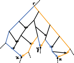
Figure 5: The frontier of an outer-labeled planar embedding of a blob is composed of an alternating succession of down- and up-paths (shown in alternating blue and orange), with one pair for each lowest node. With 3 lowest nodes in this blob $x$, $y$ and $z$ (dots), there are 3 down- and 3 up-paths. Along these paths are all four combinations of tree/hybrid articulation/non-articulation nodes. Node $y$ illustrates subcase 1 in the proof of Theorem 5.3, as a lowest node that augments the blob and is is separated from the blob’s LSA by lowest nodes along the frontier. Node $z$ illustrates subcase 2 as a augmenting lowest node between the LSA of the blob and another lowest node along the frontier.

In the first subcase, with $v$ between $u$ and $w$, the lowest nodes $u,v,w$ and any fourth articulation node $x$ on $B$ lead to an induced quartet network with a 4-blob. To see this, note this quartet network includes the three maximal biconnected sets $B_{u},B_{v},B_{w}$ containing $u,v,w$ but composed only of edges ancestral to $u,v,w$. These also contain the funnels of $u,v,w$. Moreover, since $B_{u},B_{v}$ (respectively $B_{v},B_{w}$) share the edge(s) parental to the node at which the up-paths in the frontier of $B$ from $u,v$ (respectively $v,w$) meet, $B_{u}\cup B_{v}\cup B_{w}$ is biconnected. Thus $u,v,w$ are articulation nodes on a single blob.

Varying the articulation node $x$ among the others on $B^{\prime}$ (if any exist) shows that the location of $v$ in the order from $B^{\prime}$ can be determined. Then varying $x$ among those on the funnel of $v$ shows we can determined which are on the $u$- and $w$-sides of $v$. If there is more than one articulation node, say $x_{1},x_{2}$ on $B$ between $u$ and $v$, then $u,v,x_{1},x_{2}$ induce a quartet network with a 4-blob, since these are all articulation nodes on the blob composed of edges ancestral to $u$ or $v$ (again using that in $B$ there is an edge ancestral to both $u$ and $v$). The order of $u,v,x_{1},x_{2}$ for all such $x_{1},x_{2}$ between $u$ and $v$ is sufficient to order all articulation nodes between $u$ and $v$. Similarly, the articulation nodes between $v$ and $w$ can be ordered from quartets, completing this case.

In the second subcase, where $v$ is between the blob LSA and neighboring lowest node $u$, with $w$ the other lowest node neighboring $u$ we proceed similarly. Considering $v,u,w$ and any fourth articulation node $x$ on $B$ leads to an induced quartet network with a 4-blob, as above. Varying $x$ among articulation nodes on $B^{\prime}$ determines the location of $v$ with respect to all those of $B^{\prime}$ from quartet orders. Then varying $x$ among those articulation nodes on the funnel of $v$ determines whether they lie on the LSA side or the $u$ side of $v$. Then considering induced blobs on $v,u,x_{1},x_{2}$ where the $x_{i}$ are on a common side of the funnel of $v$, is sufficient to obtain the full order. ∎

6 Circular order from genomic data

The previous section’s main result, Theorem 5.3, states that the order of branching of subnetworks around a blob can be identified from quartet information for an outer-labeled planar network. To relate this to identifiability from biological data, we discuss here several frameworks in which the 4-taxon circular order information of Definition 11 is itself identifiable, from various data types and model assumptions.

Definition 12 (gene tree models).

We consider the following models for how gene trees arise from a given rooted phylogenetic network $N^{+}$. To generate gene trees with branch lengths in substitutions per site, each edge $e$ in $N^{+}$ is assigned a length $g(e)\geq 0$ in number of generations (with $g(e)>0$ for tree edges), an effective population size $\eta(e)>0$ and a mutation rate $\mu(e)>0$ per site per generation.

1. Displayed tree (DT) model: gene trees are drawn from the set of trees displayed in $N^{+}$, with displayed tree $T$ having probability equal to the product of inheritance probabilities of all edges in $T$:

   $${\mathrm{I}\!\mathrm{P}}\!\left\{T\right\}=\gamma(T)=\prod_{e\in T}\gamma(e).$$

   Each edge $e$ in $T$ maps to a full edge in $N^{+}$ and is assigned length $\ell(e)=\mu(e)g(e)$.

2. Network multispecies coalescent model with independent inheritance (NMSCind): gene trees evolve according to the coalescent model within each population. At a hybrid node with parental edges $e_{1},\dots,e_{m}$, each lineage is inherited from population $e_{k}$ ($1\leq k\leq m$) with probability $\gamma(e_{k})$, independently of the other lineages [11]. Each gene tree edge $e^{\prime}$ formed in network edge $e$ is assigned length $\ell(e^{\prime})=\mu(e)\,g(e^{\prime})$.

3. Network multispecies coalescent model with common inheritance (NMSCcom): gene trees evolve according to the coalescent model within each population. At a hybrid node with parental edges $e_{1},\dots,e_{m}$, all lineages of a given gene are inherited from the same population $e_{k}$ ($1\leq k\leq m$), chosen with probability $\gamma(e_{k})$, and thus form within trees displayed on the network. [15]. The length of a gene tree edge is assigned as in item 2.

Under the DT model, there is no incomplete lineage sorting: lineages coalesce immediately at the time of speciation. The traditional NMSC model is what we denote NMSCind. A network coalescent model with correlated inheritance, depending on a parameter $\rho\in[0,1]$, was defined in [12], with both NMSCind ($\rho=0$) and NMSCcom ($\rho=1$) as submodels.

These gene tree models are combined with molecular substitution models, to allow for genetic sequence data. Rate variation across lineages can arise from variable sustitution rates $\mu$, and also from variable generation times, captured by a variable number of generations across different paths between the same pair of nodes. To model rate variation across genes, we further consider that each gene has a relative rate $R>0$ drawn independently from some distribution, with mean 1.

More nuanced models could be considered, in which the population size $\eta(e)$ and mutation rate $\mu(e)$ vary continuously over time instead of being considered as constant within an edge (and variable across edges). Such models would require heavier notations, but can be approximated in our framework with the addition of nodes in the network to subdivide each edge into multiple edge segments with different parameters.

Each of the following subsections considers a different type of data from these models, applying the earlier results of this work to show circular orders for blobs are identifiable. Since our focus is on identifiability, and not on inference from data, we consider only expectations associated to a data type. However, for each one, the required information can be consistently estimated from a sample of gene trees or from multilocus molecular sequences, assuming both gene sequence length and number of genes approach infinity. Thus each is potentially useful in practical inference.

6.1 Average distances from genes

The average genetic distance, or expected path length between two taxa on gene trees, is a metric that was studied in [25], and shown to be useful for identifying the tree of blobs of a network. This distance, in units of substitutions per site, is formally defined for a metric species network $N^{+}$ and one of the three gene tree models $M$ above by

$$\mathfrak{D}_{N^{+}}^{M}(x,y)={\mathrm{I}\!\mathrm{E}}\!\left(R\,D_{T}(x,y)\right),$$

where the expectation is taken over random gene trees $T$ (unscaled by gene-specific rates) generated on $N^{+}$ under model $M$, and over gene-specific relative rates $R$. Since $R$ is independent of $T$, with mean 1, this simplifies to

$$\mathfrak{D}_{N^{+}}^{M}(x,y)={\mathrm{I}\!\mathrm{E}}\!\left(D_{T}(x,y)\right).$$ (1)

For any set of 4 taxa $a,b,c,d$ and for a distance $D$ on these taxa, the 4-point distance sums-of-pairs is the vector

$$\mathrm{SP}=\mathrm{SP}_{abcd}(D)=(\mathrm{SP}_{ab|cd},\mathrm{SP}_{ac|bd},\mathrm{SP}_{ad|bc})$$

where

$$\quad\mathrm{SP}_{ab|cd}=\mathrm{SP}_{ab|cd}(D)=D(a,b)+D(c,d).$$

Recall that a distance $D$ is a tree distance if there exists a tree $T$ with edge lengths $\ell(e)$, such that for all taxon pairs $x,y$,

$$D(x,y)=D_{T}(x,y)=\sum_{e\in\mathrm{path}_{T}\;x\leftrightarrow y}\ell(e).$$

Distances on $T$ are exactly those satisfying the 4-point condition [23]: for any quartet $xy|zw$ displayed in $T$,

$$\mathrm{SP}_{xy|zw}<\mathrm{SP}_{xz|yw}=\mathrm{SP}_{xw|yz}.$$

We introduce a notion analogous to that of a (hard)-anomalous network as defined in [6] in the context of quartet concordance factors.

Definition 13.

A network $N^{+}$ is average-distance-anomalous under a model if there are two quartet trees, say $ab|cd$ and $ac|bd$, with the first displayed on $N^{+}$ and the second not, yet for the average genetic distance

$$\mathrm{SP}_{ab|cd}>\mathrm{SP}_{ac|bd}.$$

From the 4-point condition for trees one might naively suppose that the SP corresponding to some displayed quartet tree would produce the smallest SP on the quartet network. An average-distance-anomalous network is one contradicting that supposition.

Under the DT and NMSCcom models, no network is average-distance-anomalous, as follows from the next proposition. However, for the NMSCind model a network may be anomalous. Although we delay giving an example of such a network until the end of this section, this necessitates the use of the following assumption.

Assumption 2.

(NoAnomAD) Under the model NMSCind of gene tree evolution, the metric network is such that none of its induced 4-taxon networks are average-distance-anomalous.

Proposition 6.1.

Under each of the models DT, NMSCcom, and NMSCind+NoAnomAD on a rooted metric binary network $N^{+}$, average genetic distances determine the order information of 11 for each of its outer-labeled planar blobs $B$. Specifically, each induced quartet network for a $B$-informative set displays exactly 1 or 2 tree topologies, and, with taxa $a,b,c,d$:

1. If only $ab|cd$ is displayed, then $SP_{abcd}=(p,q,q)$ with $p<q$ and the quartet network on $a,b,c,d$ has a cut edge separating $a,b$ from $c,d$; and circular orders $(a,b,c,d)$ and $(a,b,d,c)$.

2. If $ab|cd$ and $ac|bd$ are displayed, then $SP_{abcd}=(p,q,r)$, with $p,q<r$ and the quartet network has a 4-blob with circular order $(a,b,d,c)$.

Proof.

Let $a,b,c,d$ be the taxa on $N^{+}$. By Lemma 5.1, we may assume either $N^{+}$ has a 4-blob, with circular order $(a,b,c,d)$, or has a cut edge separating $a,b$ from $c,d$, and hence has orders $(a,b,c,d)$ and $(a,b,d,c)$.

For the DT and NMSCcom model, the average distance on $N^{+}$ can be expressed as a weighted sum over displayed trees, denoted $S^{+}$ here (for “species” tree):

$$\mathfrak{D}_{N^{+}}^{M}(x,y)=\sum_{S^{+}}\gamma(S^{+})\;\mathfrak{D}_{S^{+}}^{M}(x,y).$$ (2)

Under the DT model, $\mathfrak{D}_{S^{+}}^{\mathrm{DT}}=D_{S^{+}}$, and under the NMSCcom model, the distance on each displayed tree is from the MSC on $S^{+}$ as a species tree: $\mathfrak{D}^{\mathrm{NMSCcom}}_{S^{+}}=\mathfrak{D}_{S^{+}}^{\mathrm{MSC}}$.

Recall that all tree edges of $N^{+}$ have positive length. Moreover, when degree-2 nodes are suppressed in a displayed tree $S^{+}$, each resulting edge arises from conjoining several edges, the highest of which must be a tree edge, yielding only positive length edges. In analyzing the above sum, then, we assume all edge lengths of $S^{+}$ are positive.

By Equation 2, it is enough to show claim 1 in the case $N^{+}=S^{+}$ is a tree. For the DT model, this is immediate from the 4-point condition, while for the NMSCind model it results from the NoAnomAD assumption. To show it holds for the MSC observe that species tree $S^{+}$ is, without loss of generality, either asymmetric, $(((a,b),c),d)$, or symmetric, $((a,b),(c,d))$. In both cases let $e$ be the edge above only $a,b$ and in the second case $\tilde{e}$ the edge above $c,d$. Under from the MSC on $S^{+}$, consider the event $E$ that a coalescence occurs on $e$ or $\tilde{e}$ (if $S^{+}$ is symmetric). Conditional on $E$, a random gene tree $T$ must have topology $ab|cd$, so that

$$\mathbb{E}(D_{T}(a,b)+D_{T}(c,d)|E)<\mathbb{E}(D_{T}(a,c)+D_{T}(b,d)|E)=\mathbb{E}(D_{T}(a,d)+D_{T}(b,c)|E).$$

Conditional on the complement $\bar{E}$, the $a,b,c$ lineages reach a common node and become exchangeable under the coalescent model, so

$$\mathbb{E}(D_{T}(a,b)+D_{T}(c,d)|\bar{E})=\mathbb{E}(D_{T}(a,c)+D_{T}(b,d)|\bar{E})=\mathbb{E}(D_{T}(a,d)+D_{T}(b,c)|\bar{E}).$$

Claim 1 then follows.

For 2 , by Lemma 5.1, if $N^{+}$ has a 4-blob it displays exactly 2 quartets, $ab|cd$ and $ac|bd$. Applying claim 1 to each displayed tree, then, we see that $\mathrm{SP}$ is a convex sum of triples of the form $(s_{i},S_{i},S_{i})$ and $(S_{i},s_{i},S_{i})$ where $s_{i}<S_{i}$ for each. Thus the last entry of $\mathrm{SP}$, corresponding to $ad|bc$, is strictly largest, establishing claim 2. ∎

Proposition 6.2.

Let $N^{+}$ be an outer-labeled planar metric rooted binary phylogenetic network. Under the DT, NMSCcom, and NMSCind+NoAnomAD models, the reduced unrooted tree of blobs of $N^{+}$ is identifiable from average genetic distances.

Proof.

For the DT model, we follow arguments from [25] who defined the distance split tree $T^{\prime}$ constructed from $\mathfrak{D}_{N^{+}}^{\mathrm{DT}}$ and the associated sums of distance pairs $\mathrm{SP}=\mathrm{SP}(\mathfrak{D}_{N^{+}}^{\mathrm{DT}})$ across all subsets of $4$ taxa. From their Theorem 8, $T^{\prime}$ is a refinement of $T$, the reduced unrooted tree of blobs of $N^{+}$. Therefore, we simply need to prove that any edge $e$ in $T^{\prime}$ is also in $T$. To prove this, we consider the split $A|B$ induced by $e$ in $T^{\prime}$. Suppose, by contradiction, that $e$ is not an edge in $T$. By Lemma 3.1.7 in [23], $e$ refines a node in $T$. In $N^{+}$, this node corresponds to an $m$-blob with $m\geq 4$, so we can select taxa $\{a_{1},a_{2},b_{1},b_{2}\}$ with $a_{1},a_{2}\in A$ and $b_{1},b_{2}\in B$ such that $N^{+}_{a_{1},a_{2},b_{1},b_{2}}$ has a $4$-blob. By the definition of the distance split tree [25], $A|B$ must satisfy the 4-point condition for $\mathfrak{D}_{N^{+}}^{\mathrm{DT}}$, so we must have that $\mathrm{SP}_{a_{1}a_{2}b_{1}b_{2}}=(s,S,S)$ with $s\leq S$. But since $N^{+}_{a_{1},a_{2},b_{1},b_{2}}$ is outer-labeled planar, $\mathrm{SP}_{a_{1}a_{2}b_{1}b_{2}}$ has a single largest entry by Proposition 6.1: a contradiction. Hence, $T=T^{\prime}$ can be identified from average distances.

Now suppose $M$ is the NMSCcom or NMSCind+NoAnomAD model. Proposition 6.1 implies that $\Sigma(\mathfrak{D}_{N^{+}}^{M})$, the set of quartet splits that satisfy the 4-point condition for metric $\mathfrak{D}_{N^{+}}^{M}$, is the same under $M$ as it is under the DT model. The distance split tree $T^{\prime}$ depends on the input distance $D$ only through $\Sigma(D)$. Therefore under $M$, $T^{\prime}$ will be the same and the rest of the argument for the DT model applies. ∎

This result extends Corollary 11 in [25] to outer-labeled planar networks of level higher than 1, and to the NMSCcom and NMSCind+NoAnomAD models, although with the restriction that the network is binary.

Combining Propositions 6.1, 6.2 and Theorem 5.3 we obtain the following.

Corollary 6.3.

Let $N^{+}$ be an outer-labeled planar metric rooted binary phylogenetic network. Then the reduced unrooted tree of blobs and the circular order for each blob on $N^{+}$ are identifiable from its average pairwise distances, under the DT, NMSCcom and NMSCind+NoAnomAD models.

Proof.

The reduced unrooted tree of blobs of $N^{+}$ is identifiable from average distances by Proposition 6.2, so we may focus on each blob individually by passing to the induced network on a subset of taxa. For every set of 4 taxa, we can determine the quartet order information of Definition 11 from average distances by Proposition 6.1. Finally, applying Theorem 5.3 completes the proof. ∎

The claims of Proposition 6.1 and the results built on it do not hold for the NMSCind model without the NoAnomAD assumption, as the following proposition shows.

Proposition 6.4.

Under the NMSCind model on an outer-labeled planar binary phylogenetic network on 4 taxa, the two smallest entries of $\mathrm{SP}$ need not indicate the circular order for a 4-blob.

Proof.

Consider the network $N$ in Figure 6 (left), considered as rooted along edge $e_{6}$, although our choice of parameters will make $\mathrm{SP}=\mathrm{SP}(\mathfrak{D}_{N}^{\mathrm{NMSCind}})$ independent of the root location. Assume for simplicity population sizes $\eta(e)=1$ and mutation rates $\mu(e)=1$ for all edges $e$, so edge lengths $g(e)=\ell(e)$ represent both coalescent units and substitutions per site. Also assume $g(e_{a})=g(e_{b})+g(e_{1})$. We will show that for sufficiently small $m$,

$$\mathrm{SP}_{ab|cd}>\mathrm{SP}_{ac|bd}>\mathrm{SP}_{ad|bc},$$

which is incompatible with the circular order $(a,b,c,d)$ in the sense that it violates the NoAnomAD Assumption 2.

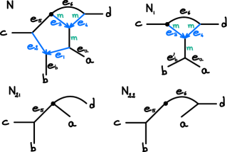
Figure 6: Example network $N$ (left) on which the claims of Proposition 6.1 do not hold under the NMSCind model, when the edge length $m$ is sufficiently small. $N_{1}$, $N_{21}$ and $N_{22}$ are displayed in $N$. The root (not shown) is on edge $e_{6}$.

For a random gene tree $T$ from the NMSCind on $N$, let $E_{1}$ denote the event that the $b$ lineage chooses $e_{1}$; $E_{21}$ the event that $b$ chooses $e_{2}$ and $a$ chooses $e_{3}$; and $E_{22}$ the event that $b$ chooses $e_{2}$ and $a$ chooses $e_{4}$. We first show that for sufficiently small $m$, we have

$${\mathrm{I}\!\mathrm{E}}\!\left(\mathrm{SP}_{ab|cd}(D_{T})\mid E_{1}\right)>{\mathrm{I}\!\mathrm{E}}\!\left(\mathrm{SP}_{ac|bd}(D_{T})\mid E_{1}\right)={\mathrm{I}\!\mathrm{E}}\!\left(\mathrm{SP}_{ad|bc}(D_{T})\mid E_{1}\right).$$ (3)

Note that the distribution of $\mathrm{SP}(D_{T})$ from $N$ conditional on $E_{1}$ is the same as the distribution of $\mathrm{SP}(D_{T})$ from the network $N_{1}$ displayed in $N$, in Figure 6. The equality in (3) follows from $N_{1}$ being symmetric with respect to $a,b$ and $g(e_{a})=g(e^{\prime}_{b})$.

To show the first inequality in (3), we consider the event $A$ that no lineages coalesce in the three edges of length $m$, and consider the expectation of $\mathrm{SP}(D_{T})$ from $N_{1}$ conditional on $A$. When $a,b$ are inherited from the same hybrid edge, $\{a,b,c\}$ or $\{a,b,d\}$ become exchangeable. By symmetry, the conditional expectation of $\mathrm{SP}(D_{T})$ then has equal entries. When $a$ and $b$ are inherited from different hybrid edges, there are several cases. When no coalescence happens on edge $e_{6}$, then $\{a,b,c,d\}$ are exchangeable above the root and by symmetry, the conditional expectation of $\mathrm{SP}(D_{T})$ has equal entries. When there is a coalescence along $e_{6}$, then $\mathrm{SP}_{ab|cd}(D_{T})=\mathrm{SP}_{ac|bd}(D_{T})$ if $a$ is inherited from $e_{4}$ and $b$ from $e_{3}$, whereas $\mathrm{SP}_{ab|cd}(D_{T})>\mathrm{SP}_{ac|bd}(D_{T})$ if $a$ is inherited from $e_{3}$ and $b$ from $e_{4}$. Since all cases above have nonzero probability, we have

$${\mathrm{I}\!\mathrm{E}}\!\left(\mathrm{SP}_{ab|cd}(D_{T})\mid E_{1}\cap A\right)>{\mathrm{I}\!\mathrm{E}}\!\left(\mathrm{SP}_{ac|bd}(D_{T})\mid E_{1}\cap A\right).$$

On the event $E_{1}\cap\bar{A}$, $T$ has topology $ab|cd$. In this case $|\mathrm{SP}_{ab|cd}(D_{T})-\mathrm{SP}_{ac|bd}(D_{T})|$ is twice the length of the internal edge of $T$, and ${\mathrm{I}\!\mathrm{E}}\!\left(|\mathrm{SP}_{ab|cd}(D_{T})-\mathrm{SP}_{ac|bd}(D_{T})|\mid E_{1}\cap\bar{A}\right)<4m+2t_{0}$, where $t_{0}=1$ is the expected time for two lineages to coalesce. Hence as $m\to 0$,

$${\mathrm{I}\!\mathrm{P}}\!\left\{\bar{A}\mid E_{1}\right\}{\mathrm{I}\!\mathrm{E}}\!\left(\left\lvert\mathrm{SP}_{ab|cd}(D_{T})-\mathrm{SP}_{ac|bd}(D_{T})\right\rvert\mid E_{1}\cap\bar{A}\right)\to 0.$$

Combining the cases for $A$ and $\bar{A}$, we have ${\mathrm{I}\!\mathrm{E}}\!\left(\mathrm{SP}_{ab|cd}(D_{T})\mid E_{1}\right)>{\mathrm{I}\!\mathrm{E}}\!\left(\mathrm{SP}_{ac|bd}(D_{T})\mid E_{1}\right)$ when $m$ is sufficiently small, establishing (3).

Next we show that for $j=1,2$, we have

$${\mathrm{I}\!\mathrm{E}}\!\left(\mathrm{SP}_{ab|cd}(D_{T})\mid E_{2j}\right)={\mathrm{I}\!\mathrm{E}}\!\left(\mathrm{SP}_{ac|bd}(D_{T})\mid E_{2j}\right)>{\mathrm{I}\!\mathrm{E}}\!\left(\mathrm{SP}_{ad|bc}(D_{T})\mid E_{2j}\right).$$ (4)

Conditional on $E_{21}$, the network becomes $N_{21}$ of Figure 6, and $T$ has topology $ad|bc$ if $b$ and $c$ coalesce on $e_{5}$, in which case $\mathrm{SP}_{ab|cd}(D_{T})=\mathrm{SP}_{ac|bd}(D_{T})>\mathrm{SP}_{ad|bc}(D_{T})$. Otherwise, $\{a,b,c\}$ are exchangeable above $e_{5}$ and the conditional expectation of $\mathrm{SP}$ has equal entries. This establishes (4) for $j=1$. For $j=2$, conditional on $E_{22}$, the same argument applies using network $N_{22}$ of Figure 6 with gene tree topology $ad|bc$ if some coalescence occurs along $e_{5}$ or $e_{6}$, or with exchangeability of $\{a,b,c,d\}$ above the root otherwise.

Combining (3) and (4), we have $\mathrm{SP}_{ab|cd}>\mathrm{SP}_{ac|bd}>\mathrm{SP}_{ad|bc}$ as desired. ∎

6.2 Quartet concordance factors

Quartet concordance factors (CFs) underlie a number of identifiability results and inference methods for level-1 networks [22, 9, 4, 1], and for the tree of blobs of general networks [2].

Under any gene tree model, quartet CFs are the probabilities, for each set of 4 taxa, of the possible gene quartet trees relating them. Since for the three models $M$ we consider (assuming a binary network in the case of DT) only resolved quartet trees have positive probability, 3-entry vectors suffice for these:

$$\mathrm{CF}_{abcd}=(\mathrm{CF}_{ab|cd},\mathrm{CF}_{ac|bd},\mathrm{CF}_{ad|bc})=(\mathbb{P}_{M}({ab|cd}),\mathbb{P}_{M}({ac|bd}),\mathbb{P}_{M}({ad|bc})).$$

These CFs can be obtained by marginalizing the distribution of rooted metric gene trees over edge lengths, root locations, and all but 4 taxa. The model of sequence evolution on the gene trees is thus irrelevant as long as gene tree topologies are identifiable. Although CFs can be consistently estimated from a sample of gene trees, in practice such a sample is never available, so they are estimated from inferred gene trees or directly from multilocus sequence data.

Following [6], we say a 4-taxon network $N^{+}$ is (hard-)anomalous when there are two quartet trees, say $ab|cd$ and $ac|bd$, with the first displayed on $N^{+}$ and the second not, yet

$$\mathrm{CF}_{ab|cd}<\mathrm{CF}_{ac|bd}.$$

More informally, a network is anomalous if the displayed tree(s) are not the most probable gene trees.

Under the DT model on a 4-taxon network, only the trees displayed on the network have positive probability, so no anomaly can occur. Under the NMSCcom model, all binary gene trees have positive probability but, by Proposition 12 of [6], there are again no anomalies.

Anomalies can occur under the NMSCind model, although only one embedded network substructure (a $3_{2}$-cycle) is currently known to lead to them. However, even with such a substructure, an anomaly does not occur for all parameter values on the network. See Proposition 1 of [2] for an extreme example of an anomalous outer-labeled planar network displaying a single tree topology, and [6] for deeper investigations and simulations on the frequency of anomalies.

To identify circular orders of an outer-labeled planar network under NMSCind from CFs, we use the following:

Assumption 3.

(NoAnomQ) Under the model NMSCind of gene tree evolution, the metric network is such that none of its induced 4-taxon networks are anomalous.

We first show that under our three models, assuming no anomalous 4-networks, CFs determine the quartet order information of 11.

Proposition 6.5.

Under each of the models DT, NMSCcom, and NMSCind+NoAnomQ on a rooted metric binary network, quartet CFs determine the order information of 11 for each of its outer-labeled planar blobs $B$. Specifically, each induced quartet network for a $B$-informative set displays exactly 1 or 2 tree topologies, and, with taxa $a,b,c,d$:

1. If only $ab|cd$ is displayed, then $\mathrm{CF}_{abcd}=(p,q,q)$ with $p>q$ and the quartet network on $a,b,c,d$ has a cut edge separating $a,b$ from $c,d$; and circular orders $(a,b,c,d)$ and $(a,b,d,c)$.

2. If $ab|cd$ and $ac|bd$ are displayed, then $\mathrm{CF}_{abcd}=(p,q,r)$, with $p,q>r$ and the quartet network has a 4-blob with circular order $(a,b,d,c)$.

Proof.

From Lemma 5.1, an induced quartet network displays either 1 or 2 tree topologies, depending on whether it lacks or has a 4-blob. If it lacks a 4-blob, it has a cut edge separating the taxa into groups of two, which must be $a,b$ and $c,d$ if $ab|cd$ is displayed.

If a quartet network displays only the tree topology $ab|cd$, then under the DT model, $\mathrm{CF}_{abcd}=(1,0,0)$, since for each displayed tree the CF is $(1,0,0)$. Likewise, under NMSCcom, $\mathrm{CF}_{abcd}=(p,q,q)$ with $p>q$, since for each displayed tree the CF has this form [5]. For NMSCind, Theorem 1 of [2] implies $\mathrm{CF}_{abcd}=(p,q,q)$, and $p>q$ follows from the assumption NoAnomQ.

If a quartet network displays 2 tree topologies, $ab|cd$ and $ac|bd$, then $\mathrm{CF}_{abcd}=(p,q,r)$ with $p,q>r$ is shown for the DT and NMSCcom models by similarly considering the displayed trees individually. For the NMSCind model, this follows from the NoAnomQ assumption. ∎

Corollary 6.6.

Let $N^{+}$ be a rooted metric binary phylogenetic network. Then under the models DT, NMSCcom, and NMSCind+NoAnomQ models the reduced unrooted tree of blobs and the circular order for each outer-labeled planar blob on $N^{+}$ are identifiable from quartet CFs.

Proof.

Under NMSCind, the reduced unrooted tree of blobs of $N^{+}$ is identifiable from CFs by Proposition 4 of [2], for generic parameters. One can check that with the NoAnomQ assumption, the generic condition can be dropped, since it is used only in the determination of 4-taxon sets whose subnetwork has a 4-blob, which can instead be determined by Theorem 6.5.

Similarly, for DT and NMSCcom, Theorem 6.5 allows the arguments of [2] to apply, to prove the identifiability of the tree of blobs from CFs.

Theorems 6.5 and 5.3 then show each outer-labeled planar blob’s circular order is identifiable. ∎

6.3 LogDet distances from genomic sequences

In [7, 3], logDet distances computed from genomic sequences were shown to identify species trees and level-1 network topologies under an independent coalescent model, provided certain technical assumptions hold. This information differs from the average distances considered in Section 6.1, since the logDet distance is computed from concatenated multigene sequences, as opposed to sequences for each gene individually. Here we study using LogDet distances to identify circular orders of blobs in outer labeled planar networks.

Recall that a rooted metric network is said to be ultrametric if all paths from the root to a leaf have the same length. An ultrametric network is therefore time-consistent, in the sense that for every node $u$, all the paths from the root to $u$ have the same length.

In this subsection we consider only rooted networks that are ultrametric when edge lengths are measured in generations. We also assume a mutation rate that is constant across all edges, so ultrametricity in substitution units holds as well. (For simplicity, we do not investigate generalization to time-dependent mutation rates, or to varying substitution processes across genes, as in [7, 3].)

The requirement that a network be ultrametric is tied to the use of rooted triples, rather than quartets, for identifiability. In particular, triples of logDet distances from each displayed rooted triple network play a similar role to the CF triples for displayed quartets. We thus require results and definitions paralleling those of earlier sections, with rooted triple networks replacing quartet networks. Since many of the necessary arguments are straightforward adaptations of those for quartets, we omit many details and only highlight key differences.

We strengthen the definition of an outer-labeled planar blob in a rooted network by considering the extended articulation nodes $\widetilde{V}_{0}$ as the usual articulation nodes together with the blob’s LSA. A blob is extended outer-labeled planar if it is outer-labeled planar with respect to $\widetilde{V}_{0}$. In this subsection we use the term $m$-blob to refer to a blob with $m$ extended articulation nodes.

If a blob does not contain the network root then the blob’s LSA must be an articulation node, so ‘extended outer-labeled planar’ is synonymous with ‘outer-labeled planar’. These terms have different meanings only for blobs containing the network root, since the extended definition requires a planar embedding with the root in the frontier, while the standard definition does not.

Applying Theorem 4.1 to $\widetilde{V}_{0}$ immediately yields the following.

Corollary 6.7.

There is a unique circular order of the extended articulation nodes of an extended outer-labeled planar blob of a rooted phylogenetic network, induced from every extended outer-labeled planar embedding of the blob.

Definition 14.

For a blob $B$ in a rooted phylogenetic network, a 3-taxon set is $B$-informative if its elements are in distinct taxon blocks associated to $B$, excluding the block associated to the blob’s LSA. A collection of 3-taxon sets is a full $B$-informative collection if, for each choice of 3 blocks of $B$ not associated to its LSA, one of the 3-taxon sets contains a taxon from each block.

If $B$ is an extended outer-labeled planar blob, then the 3-taxon network induced by a $B$-informative set of 3 taxa need not have the same LSA as $B$. Nonetheless, since there can only be a chain of 2-blobs between the LSA of the 3 taxa and the LSA of $B$, whichever LSA we refer to has no impact on the notion of circular order information in the following.

Definition 15.

For an extended outer-labeled planar blob $B$ with LSA $L=L_{B}$ in a binary rooted phylogenetic network and a full $B$-informative collection of 3 taxon sets, the 3-taxon circular order information is the collection of circular orders of $x,y,z,L$ specified by the induced rooted triple networks for the 3-taxon sets $\{x,y,z\}$. More specifically, this information consists of all circular orders of $x,y,z,L$ that are compatible with all unrooted displayed trees in the rooted 3-taxon network:

1. for a rooted triple network without a 4-blob, and hence a cut edge inducing a split $xy|zL$ of the taxa and LSA, the circular orders are $(x,y,z,L)$ and $(x,y,L,z)$.

2. for a rooted triple network with a 4-blob, the circular order is the unique order induced from any extended outer-labeled planar embedding of the rooted triple network.

The following is an analog for rooted triples of Theorem 5.3. Unfortunately, it cannot be immediately deduced from that quartet result, since even extending the rooted network with an additional outgroup taxon, there are fewer collections of 3 ingroup taxa than there are collections of 4 taxa.

Theorem 6.8.

Let $B$ be an extended outer-labeled planar blob in a rooted binary phylogenetic network. Then 3-taxon circular order information on a full $B$-informative set of 3-taxon sets determines the unique circular order of its extended articulation nodes induced by all outer-labeled planar embeddings of the blob.

Proof.

Our argument parallels that for Theorem 5.3, so we only provide a sketch.

Proceeding by induction on the number of lowest nodes of $B$, if $v$ is the only lowest node, then for every choice of articulation nodes $x,y$ we have a unique circular order for $v,x,y,L$ which must be congruent with the unique circular order of the full set $\widetilde{V}_{0}$ of the extended articulation nodes. It is straightforward to see the orders for all choices of $x,y$ determine that for $\widetilde{V}_{0}$.

Assuming the result for any blob with $n-1$ lowest nodes, suppose that $B$ has $n$, and pick an augmenting lowest node $v$. With $B^{\prime}$ obtained from $B$ by deleting $v$ and its funnel, the circular order for the extended articulation nodes of $B^{\prime}$, which has $n-1$ lowest nodes, is determined by induction. Note that $L$ must be in $B^{\prime}$ since $v$ is augmenting, hence $L$ is included in this order.

If $B^{\prime}$ has a single lowest node $u$, then since all edges of $B$ are ancestral to $u$ or $v$, the rooted network induced by $u,v,x$ has a 4-blob for any other articulation node $x$ of $B$. Letting $x$ vary over articulation nodes of $B^{\prime}$ determines a unique placement of $v$ within the circular order for $B^{\prime}$. Then, letting $x$ vary over articulation nodes of $B$ on the funnel of $v$ determines the position of each one relative to $v$ and to articulation nodes of $B^{\prime}$ (including $L$). What remains to be determined is the position of these articulation nodes on the funnel relative to one another. But by restricting to the blob containing $v$ in the induced network on those taxa which are descended from the funnel of $v$, which has only one lowest node, a unique circular order for all articulation nodes on the funnel of $v$ can also be determined.

If $B^{\prime}$ has more than one lowest node, using rooted triple order information we first determine where $v$ should be placed between other lowest nodes and the blob LSA $L$, and then argue as in the last case to obtain the full circular order. ∎

Recall the definition of the logDet distance between two (finite) aligned sequences of $k$ bases from taxa $a,b$ [24]. Let $F_{ab}$ be the $k\times k$ matrix of relative site-pattern frequencies, whose $ij$ entry gives the proportion of sites in the sequences exhibiting base $i$ for $a$ and base $j$ for $b$. Let $f_{a}$ denote the vector of row sums of $F_{ab}$, and $f_{b}$ the vector of column sums, so that these marginalizations give the proportions of various bases in the sequences of $a$ and $b$. With $g_{a}$ and $g_{b}$ the products of the entries of $f_{a},f_{b}$, respectively, the logDet distance is

$$d_{ab}=-\frac{1}{k}\left(\ln|\det(F_{ab})|-\frac{1}{2}\ln(g_{a}g_{b})\right).$$

Instead letting $F_{ab}$ be the matrix of expected genomic pattern frequencies from a model $M$ on a rooted network $N^{+}$, this formula yields a logDet distance determined by the model’s distribution of genomic sequence data. It is from these distances that we seek to identify circular orders for blobs. With $d^{M}_{xy}$ the logDet distance computed from expected genomic pattern frequencies for taxa $x,y$ under model $M$, let

$$D_{abc}=D^{M}_{abc}=(d^{M}_{ab},d^{M}_{ac},d^{M}_{bc})$$

be the triple of pairwise distances between three taxa $a,b,c$.

The following is an extension of results for a level-1 ultrametric network in [3], which can be proved similarly to Theorem 1 of [2].

Proposition 6.9.

Consider a 3-taxon ultrametric rooted binary network with LSA $L$. For the DT, NMSCcom, and NMSCind models with constant mutation rate and generic numerical parameters, if the network has a 4-blob then the three entries of $D_{abc}$ are distinct, while if there is an internal cut edge separating $a,b$ from $c,L$ then $d_{ac}=d_{bc}$.

Proof.

If the network on $a,b,c$ has a 4-blob, a modification of the topological argument in the proof of Theorem 1 of [2] shows it displays a level-1 network with a 4-blob. Choosing hybridization parameters in such a way that lineages are constrained to stay in this displayed network, Theorem 1 of [3] shows that for NMSCind the three entries of $D_{abc}$ are distinct for generic parameters on the displayed network. Since these entries are analytic functions of the parameters for the full network, for generic parameters on the full network they must also be distinct. For the DT and NMSCcom model, a similar argument applies, though showing the analog of Theorem 1 of [3] holds for them requires a detailed application of the algebraic Lemma 4 of [7] to pattern frequency matrices.

If there is an internal cut edge separating $a,b$ from $c$ on the network, then under any of these models for each possible gene tree there is an equiprobable gene tree obtained by interchanging the $a,b$ labels, by ultrametricity. This implies the expected pattern frequency arrays for $a,c$ and for $b,c$ are the same, so $d_{ac}=d_{bc}.$ ∎

It is also straightforward to follow the arguments of [2], replacing its use of the combinatorial quartet distance capturing topological information on quartets separating pairs of taxa by the rooted triple distance of [21], to obtain the following.

Proposition 6.10.

The reduced rooted tree of blobs of a rooted binary network can be determined from the reduced rooted trees of blobs for each of its induced rooted 3-taxon networks.

The notion of an unrooted 4-taxon anomalous network for quartet CFs has a parallel for logDet distances.

Definition 16.

An ultrametric rooted triple network $N^{+}$ is logDet-anomalous for a model $M$ if there are two rooted triple trees, say $ab|c$ and $ac|b$, with the first displayed on $N^{+}$ and the second not, yet

$$d_{ab}^{M}>d_{ac}^{M}.$$

This notion captures the naive idea that a taxon pair appearing as a cherry on a displayed tree should appear to have more closely related sequences than if they are not a cherry on any displayed tree. This idea is used by [19] to define a “species-definition anomaly” zone, in which $a$ and $b$ are two individuals from the same species and $c$ is an individual from a different species.

From [7], an ultrametric tree $((a,b),c)$ is never logDet-anomalous for the MSC model since $d_{ab}<d_{ac}=d_{bc}$. However, as shown in [3], there are level-1 rooted triple networks with tree of blobs $((a,b),c)$ yet $d_{ab}>d_{ac}=d_{bc}$, although known examples require extreme parameters. However, the question of what network structures can lead to logDet anomalies and how common they might be has not been investigated in depth.

To identify circular orders of extended outer-labeled planar blobs in a binary network from logDet distances under the NMSCind model, we will use the following:

Assumption 4.

(NoAnomLD) Under the NMSCind model, the metric network is such that none of its induced 3-taxon rooted networks are LogDet-anomalous.

Proposition 6.11.

Under each of the models DT, NMSCcom, and NMSCind+NoAnomLD with constant mutation rate on a binary rooted ultrametric network with generic numerical parameters, logDet distances determine the order information of Definition 15 for each of its extended outer-labeled planar blobs $B$. Specifically, each induced rooted triple network for a $B$-informative set displays exactly 1 or 2 tree topologies. For taxa $a,b,c$ and blob LSA $L$:

1. If only $ab|c$ is displayed, then $D_{abc}=(p,q,q)$ with $p<q$ and the rooted triple network on $a,b,c$ has an internal cut edge separating $a,b$ from $c$; and circular orders $(a,b,c,L)$ and $(b,a,c,L)$.

2. If $ab|c$ and $ac|b$ are displayed, then $D_{abc}=(p,q,r)$, with $p,q<r$ and the quartet network has a 4-blob with circular order $(a,b,L,c)$.

Proof.

Attaching a new outgroup taxon at the root and applying Lemma 5.1 shows an induced rooted triple network displays either 1 or 2 tree topologies, depending on whether it lacks or has a 4-blob. Moreover, the network must have an internal cut edge $e$ separating $a,b$ from $c$ if only $ab|c$ is displayed.

If a rooted triple network displays only the tree topology $ab|c$, then for all three models 6.9 shows $D_{abc}=(p,q,q)$. For the DT and NMSCcom model one can show $p<q$ using the algebraic Lemma 4 of [7] with an analysis of pattern frequency arrays on each displayed tree, similar to Theorem 8 of that work. For NMSCind, that $p<q$ follows from the assumption NoAnomLD.

If a rooted triple network displays 2 tree topologies, $ab|c$ and $ac|b$, then $D_{abc}=(p,q,r)$ by 6.9. That $p,q<r$ is shown for the DT and NMSCcom models by considering the displayed trees individually and using Lemma 4 of [7]. For the NMSCind model, that $p,q<r$ follows from the NoAnomLD assumption. ∎

Corollary 6.12.

Let $N^{+}$ be a rooted metric binary ultrametric phylogenetic network, with generic parameters. Then under the models DT, NMSCcom, and NMSCind+NoAnomLD models, the reduced rooted tree of blobs and the circular order for each extended outer-labeled planar blob on $N^{+}$ are identifiable from logDet distances.

Proof.

The tree of blobs for each triple of taxa is identifiable by 6.9, and hence for the full network by 6.10. 6.11 and Theorem 6.8 give the identifiability of circular orders for extended outer-labeled planar blobs. ∎

7 Identifiability limits beyond the circular order

We now argue that from the data types and models considered in the previous section the circular order for outer labeled planar blobs may be close to the strongest topological information that one can identify. We do this by exhibiting outer-labeled planar networks with distinct topologies that have the same pairwise average genetic distances, quartet CFs, or logDet distances. We similarly show that distinguishing between outer-labeled planar networks and non outer-labeled planar networks is not always possible via these data types.

Some such non-identifiability results have been found previously. Even level-1 4-taxon network topologies are not always distinguishable from one-another [22, 9, 25]. In any network, a 2-blob may be replaced with a single tree edge without affecting quartet CFs nor average distances [6, 25]. Also 3-blobs may be shrunk into a single 3-taxon subtree without affecting average distances [25], and in some level-1 cases be shrunk or have their hybrid node moved without affecting CFs [1].

Our new examples of indistinguishable networks have larger blobs, including ones of high level. While some of these are outer-labeled planar and thus have the same identifiable circular order, others are not. The fact that they are nonetheless associated with a unique circular order suggests that it may be possible to meaningfully generalize the notion of circular order beyond the class of outer-labeled planar networks.

7.1 Limits of identifiability from average distances

We present here a class of 5-taxon networks that are indistinguishable from a network with a single reticulation, based on average distances under the DT model and NMSCcom models. This includes the networks in Figure 9, but also others such as in Figure 7.

Proposition 7.1.

Let $M$ be the DT or NMSCcom model. Let $N$ be a metric binary network on $\{a,b,c,d,h\}$ such that:

1. $N$ contains a 5-blob.

2. The subnetwork $N_{\{a,b,c,d\}}$ contains a cut edge that induces the split $ad|bc$.

3. The degree-2 nodes in $N_{\{a,b,c,d\}}$ at which paths to $h$ last leave $N$ all lie on an up-down path from $a$ to $b$, and all are incident to two cut edges in $N_{\{a,b,c,d\}}$.

If the edges incident to $a$ and $b$ in $N$ are sufficiently long, then the average distances on $N$ also fit a 5-sunlet $N_{1}$ as shown in Figure 7 left: $\mathfrak{D}_{N}^{M}=\mathfrak{D}_{N_{1}}^{M}$.

Figure 7: $N$ (left) is an example network satisfying the conditions of 7.1. It is indistinguishable from the level-1 network $N_{1}$ (right) using average distances under the DT or NMSCcom model provided the pendent edges to $a$ and $b$ are sufficiently long. Orange edges of $N$ are absent from $N_{abcd}$, which is shown in black. $N_{1}$ is a $5$-sunlet, that is, has 5 taxa and a single 5-cycle. Edge lengths, in black, are in substitutions per site ($\mu(e)g(e)$ in Def. 12). Hybrid edges and their $\gamma$s are shown in blue.

Our proof proceeds by establishing two claims: First, the trees displayed on $N$ have 2 or 3 distinct unrooted topologies, shown in Figure 8. Second, if a network $N$ displays these topologies, then its average distances fit a 5-sunlet. For this second step, we establish several lemmas.

Figure 8: Topologies of trees displayed on $N$ under the conditions in 7.1. The left and middle topologies must be displayed. The right topology may or may not be displayed.

Lemma 7.2.

Let $N_{1}$ be the 5-sunlet with parameters as shown in Figure 7 (right), $\mathfrak{D}=\mathfrak{D}_{N_{1}}^{M}$ and $\mathrm{SP}=\mathrm{SP}(\mathfrak{D})$, where $M$ is the DT model or the NMSCcom model with an expected number of substitutions per coalescent unit $s=\mu(e)\eta(e)$ constant across edges $e$ in $N_{1}$. Then

$$2t_{0} =\mathrm{SP}_{ac|bd}-\mathrm{SP}_{ad|bc} 2t_{a} =(\mathrm{SP}_{ab|hd}-\mathrm{SP}_{ah|bd})/\gamma_{b}$$ (5)

$$\gamma_{b} =(\mathrm{SP}_{bd|ch}-\mathrm{SP}_{bc|dh})/(2t_{0}) 2t_{b} =(\mathrm{SP}_{ba|hc}-\mathrm{SP}_{bh|ac})/\gamma_{a}$$

and for $j=a,b,c,d,h$, $\mu_{j}=\hat{\mu}_{j}$ under the DT model or $\mu_{j}=\hat{\mu}_{j}-s$ under the NMSCcom model, where

$$2\hat{\mu}_{c} =\mathfrak{D}(c,b)+\mathfrak{D}(c,d)-\mathfrak{D}(b,d) 2\hat{\mu}_{h} =\mathfrak{D}(a,h)+\mathfrak{D}(b,h)-\mathfrak{D}(a,b)$$ (6)

$$2\hat{\mu}_{d} =\mathfrak{D}(d,a)+\mathfrak{D}(d,c)-\mathfrak{D}(a,c) 2\hat{\mu}_{j} =\mathfrak{D}(j,c)+\mathfrak{D}(j,d)-\mathfrak{D}(c,d)-2t_{j}\mbox{ {for} }j\in\{a,b\}\,.$$

Furthermore, given a metric $D$ on $\{a,b,c,d,h\}$, there exists a 5-sunlet $N_{1}$ as in Figure 7 (right), such that $D=\mathfrak{D}_{N_{1}}^{M}$, if and only if the following holds, denoting $\mathrm{SP}=\mathrm{SP}(D)$:

1. $D$ satisfies the triangle inequality strictly.

2. $D$ satisfies the strict 4-point condition $\mathrm{SP}_{ad|bc}<\mathrm{SP}_{ac|bd}=\mathrm{SP}_{ab|cd}$.

3. On each 4-taxon subset, $D$ is compatible with the circular order $(a,d,c,b,h)$:

   $$\begin{split}\mathrm{SP}_{bd|ch}>\max\{\mathrm{SP}_{bc|dh},\mathrm{SP}_{bh|cd}\},&\quad\mathrm{SP}_{ac|dh}>\max\{\mathrm{SP}_{ad|ch},\mathrm{SP}_{ah|cd}\}\\ \mathrm{SP}_{ab|dh}>\max\{\mathrm{SP}_{ad|bh},\mathrm{SP}_{ah|bd}\},&\quad\mathrm{SP}_{ab|ch}>\max\{\mathrm{SP}_{ac|bh},\mathrm{SP}_{ah|bc}\}\end{split}$$

4. $\hat{\mu}_{a}>0$ and $\hat{\mu}_{b}>0$ where $\hat{\mu}_{a}$ and $\hat{\mu}_{b}$ are calculated from $D$ using (5) and (6).

Note that in each equation of (5) and (6), the right-hand-side involves only distances and terms given by preceding equations. Therefore they allow for all parameter values to be found from pairwise distances.

Proof.

By expressing the distances $\mathfrak{D}=\mathfrak{D}_{N_{1}}^{\mathrm{DT}}$ in terms of parameters $t_{i},\mu_{j},\gamma_{b}$ where $i=0,a,b$ and $j=a,b,c,d,h$, (5) and (6) with $\hat{\mu}_{j}=\mu_{j}$ can be verified by calculation. For $\gamma_{b}$, an intermediate but equivalent expression is $2\gamma_{b}-1=(\mathfrak{D}(c,h)-\mathfrak{D}(d,h)-\mu_{c}+\mu_{d})/t_{0}$.

Under the NMSCcom model, $\mathfrak{D}=\sum_{T}\gamma(T)\;\mathfrak{D}_{T}^{\mathrm{MSC}}$ is a weighted sum over displayed trees. On a tree $T$, assuming a constant mutation rate per coalescent unit $s=\mu\eta$, we get $\mathfrak{D}_{T}^{\mathrm{MSC}}(x,y)=\mathfrak{D}_{T}^{\mathrm{DT}}(x,y)+2s$, where the extra $2s$ is the average number of substitutions after 2 lineages reach a common population (going back in time) as it takes an average of 1 coalescent unit for two lineages to coalesce. Then $\mathfrak{D}_{N_{1}}^{\mathrm{NMSCcom}}=\mathfrak{D}_{N_{1}}^{\mathrm{DT}}+2s$ and $\mathrm{SP}^{\mathrm{NMSCcom}}=\mathrm{SP}^{\mathrm{DT}}+4s$. Therefore (5) for DT implies (5) for NMSCcom. Also, (6) with $\hat{\mu}_{j}=\mu_{j}$ for the DT model implies (6) for the NMSCcom model with $\hat{\mu}_{j}=\mu_{j}+s$: pendent edge lengths are overestimated by the average number of substitutions between speciation and coalescent times.

For the second part, $\mathfrak{D}$ satisfies (a) because pendent edges, being tree edges, are assumed of positive length. $\mathfrak{D}$ satisfies (b-c) by 6.1 and (d) by the first part. Conversely, let $D$ be a metric satisfying (a-d). Then we apply (5) to obtain “fitted” parameters $\hat{t}_{i}$ ($i=0,a,b$) and $\hat{\gamma}=\hat{\gamma}_{b}$, and (6) to obtain $\hat{\mu}_{j}$ ($j=a,b,c,d,h$). We now show that these parameters are valid, that is: $\hat{t}_{i}>0$, $0<\hat{\gamma}<1$ and $\hat{\mu}_{j}>0$.

We have $\hat{\mu}_{a},\hat{\mu}_{b}>0$ by (d). By (a), $\hat{\mu}_{h},\hat{\mu}_{c},\hat{\mu}_{d}>0$. From (5) we get $\hat{t}_{0}>0$ by (b) and $\hat{\gamma}>0$ by (c). Similarly, $\hat{\gamma}_{a}=1-\hat{\gamma}>0$ and consequently $0<\hat{\gamma}<1$. Finally, $t_{a},t_{b}>0$ by (c). $N_{1}$ can then be assigned these fitted parameters, and by the first part, $\mathfrak{D}_{N_{1}}^{\mathrm{DT}}=D$. Under the NMSCcom model, let $s=\min_{j=a,b,c,d,h}\{\hat{\mu}_{j}/2\}>0$. To edge $e$ in $N_{1}$ we assign $\mu(e)=1$ mutation per generation, population size $\eta(e)=1/s$, and length $g(e)$ generations such that the expected number of substitutions $\mu(e)g(e)$ equals $t_{i}$ ($i=0,a,b$) for internal edges or $\hat{\mu}_{j}-s>0$ ($j=a,b,c,d,h$) for pendent edges. Then by the first part, $\mathfrak{D}_{N_{1}}^{\mathrm{NMSCcom}}=D$. ∎

Lemma 7.3.

Let $M$ be the DT or NMSCcom model. Let $N$ be a binary network on $\{a,b,c,d,h\}$. Assume that every tree displayed in $N$, after suppressing degree-2 nodes, has one of the topologies shown in Figure 8, with the left and middle topologies both displayed. If the pendent edges to $a,b$ in $N$ are sufficiently long, then $\mathfrak{D}_{N}^{M}=\mathfrak{D}_{N_{1}}^{M}$ for a 5-sunlet $N_{1}$.

Proof.

We will show that $D=\mathfrak{D}_{N}^{M}$ satisfies (a-d) of Lemma 7.2. $D$ is a convex combination of $\mathfrak{D}_{T}^{M}$ for trees $T$ displayed in $N$. For each displayed tree $T$, $\mathfrak{D}_{T}^{M}$ satisfies (a-b) so $D$ does too. Each expression in (c) is equivalent to two inequalities, such as $\mathrm{SP}_{bd|ch}>\mathrm{SP}_{bc|dh}$ and $\mathrm{SP}_{bd|ch}>\mathrm{SP}_{bh|cd}$. Non-strict versions of both inequalities hold for all displayed trees by 6.1, with the strict inequality holding for either the left or the middle tree topology. Averaging over displayed trees shows the inequalities hold strictly for $D$.

For the final condition (d), we note that when the length of the pendent edge to $a$ (resp. $b$) is increased by some amount, $\hat{\mu}_{a}$ (resp. $\hat{\mu}_{b}$) increases by the same amount, and all other fitted parameters are unchanged. Hence, for sufficiently long pendent edges to $a$ and $b$, (d) is satisfied. The conclusion then follows from Lemma 7.2. ∎

To prove that the conditions of 7.1 imply the assumptions of Lemma 7.3, a few more definitions will be useful.

Definition 17.

Let $N$ be a network on $X$, and $x\in X$. We write $N_{\setminus x}$ for the induced subnetwork on ${X\setminus\{x\}}$. An attachment node of $x$ in $N$ is a node $u$ in $N_{\setminus x}$ that is, in $N$, incident to an edge $e\notin E(N_{\setminus x})$. The edge $e$ is called an attachment edge.

Lemma 7.4.

Let $N$ be a binary network on 5 taxa. If all its unrooted displayed trees share the same non-trivial split, then $N$ has a cut edge corresponding to that split.

Proof.

If $N$ has no $4$- or $5$-blob, the result is trivial, since all trees displayed in $N$ have the same unrooted topology as $N$’s tree of blobs, whose edges arise from $N$’s cut edges.

Suppose then that $N$ has a $4$-blob. Let $S=a_{1}a_{2}|a_{3}a_{4}a_{5}$ be a split in all trees displayed on $N$. Since $N$ has a $4$-blob, it has an internal cut edge. If this cut edge corresponds to $S$, we are done. Otherwise, this cut edge is compatible with $S$ because it is present in the displayed trees. Without loss of generality, assume that this cut edge corresponds to $a_{1}a_{2}a_{3}|a_{4}a_{5}$, in which case all trees displayed in $N$ have the same unrooted topology (after removing degree-2 nodes) and $N^{\prime}=N_{\setminus a_{5}}$ has a 4-blob. But by Lemma 5.1 $N^{\prime}$ cannot have a 4-blob since all its unrooted displayed trees share the same split.

Now suppose $N$ has a $5$-blob, and let $v$ be a lowest hybrid node in the blob. Since $N$ is on $5$ taxa, $v$ has exactly one descendent taxon, say $a_{1}$. Assume the split on all displayed trees is $S=a_{1}a_{2}|a_{3}a_{4}a_{5}$ or $S=a_{1}a_{2}a_{3}|a_{4}a_{5}$. In the former case we prune $x=a_{5}$ from $N$ and in the latter case we prune $x=a_{3}$, to consider $N^{\prime}=N_{\setminus x}$. Then $N^{\prime}$ has a $4$-blob yet all its displayed trees have split $a_{1}a_{2}|a_{3}a_{4}$, which contradicts Lemma 5.1. ∎

Proof of 7.1.

Let $N$ be a network satisfying the conditions of 7.1. By Lemma 7.3, we just need to show that its unrooted displayed trees, after suppressing degree-2 nodes, have one of the topologies in Figure 8, and that the first two topologies are displayed in $N$. Let $T$ be a tree displayed in $N$. Then $T_{\setminus h}$ is a tree displayed in $N_{\setminus h}$. It must contain cut edges from $N_{\setminus h}$, so by assumption 2 it contains an edge of positive length corresponding to the split $ab|cd$.

Let $v$ be the attachment node of $h$ in $T$. We claim that $v$ is an attachment node of $h$ in $N$ as well. Let $h=v_{0},v_{1},\cdots,v_{k}=v$ be the path from $h$ to $v$ in $T$, and let $v_{j}$ be the first node along this path to be in $N_{\setminus h}$. Then $(v_{j},v_{j-1})$ (or $(v_{j-1},v_{j})$) is not in $N_{\setminus h}$ and $v_{j}$ is an attachment node of $h$ in $N$. By assumption 3 and since $N$ is binary, $v_{j}$ is incident to 2 cut edges in $N_{\setminus h}$ and to the attachment edge $(v_{j},v_{j-1})$. All 3 edges are then in $T$, because $T_{\setminus h}$ must contain all cut edges in $N_{\setminus h}$. Therefore $v_{j}$ has degree 3 in $T$, $j=k$, and $v$ is an attachment node of $h$ in $N$. Since $v$ is a cut node in $N_{\setminus h}$, and by assumption 3, $v$ must be on every up-down path between $a$ and $b$ in $N_{\setminus h}$. In particular, $v$ is also on the path between $a$ and $b$ in $T_{\setminus h}$. This ensures that $T$ has one of the topologies in Figure 8 (after suppressing degree-2 nodes).

It remains to show that $N$ displays the left and middle topologies of Figure 8. By assumption 3, only these three trees could be displayed on $N$. By assumption 1, $N$ has a $5$-blob, so Lemma 7.4, implies the trees displayed on $N$ cannot all share a non-trivial split. This rules out only one tree being displayed, only the left and right trees (which share $hbc|da$) being displayed, and only the middle and right trees (which share $bc|dah$) being displayed. Thus either the left and middle trees, or all three trees, are displayed on $N$. Applying Lemma 7.3 completes the proof. ∎

7.2 Limits of identifiability from quartet concordance factors

In this section, we present a family of 5-taxon networks with 5-blobs, some outer-labeled planar and some not, which are indistinguishable from a network with a single reticulation using quartet CFs under the DT, NMSCcom, and NMSCind models. This family, illustrated in Figure 9, is a subset of the class considered in 7.1.

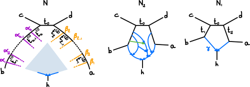
Figure 9: Example networks that are not distinguishable from quartet CFs. $N$ (left) shows the general structure of a binary network on $\{a,b,c,d,h\}$ with $N_{\{a,b,c,d\}}$ the tree $ab|cd$ with extra degree-2 nodes on the pendent edges to $a,b$. At these nodes all paths to $h$ connect. $N_{1}$ (right, outer-labeled planar level-1) and $N_{2}$ (middle) have this structure. $N_{2}$ is not outer-labeled planar, but would be without the green edge. These networks display the same two tree topologies.

Proposition 7.5.

Let $M$ be the DT, NMSCcom, or NMSCind model. Let $N$ be a metric binary network on $\{a,b,c,d,h\}$ such that:

1. The subnetwork $T=N_{\{a,b,c,d\}}$ is a tree with a cut edge that induces the split $ad|bc$.

2. The degree-2 nodes in $T$ at which paths to $h$ last leave $N$ all lie on the pendent edges to $a$ or to $b$ in the reduced tree.

As labelled in Figure 9 (left), let $\alpha_{i}$ and $\beta_{j}$ be the probabilities that a lineage from $h$ traces its ancestry back to specific degree-2 nodes in $T$, and let $t_{i}^{(1)}$ and $t_{j}^{(2)}$ be the lengths of edges between these nodes. Let $N_{1}$ be the 5-sunlet with topology and parameters as depicted in Figure 9 (right). If $t_{1}$, $t_{2}$, and $\gamma$ are such that $\gamma=\sum_{i=1}^{k}\alpha_{i}$,

$$\gamma e^{-t_{1}}=\sum_{i=1}^{k}\alpha_{i}e^{-\sum_{j=i}^{k}t^{(1)}_{j}},\;\mbox{ and }\quad(1-\gamma)e^{-t_{2}}=\sum_{i=1}^{\ell}\beta_{i}e^{-\sum_{j=i}^{\ell}t^{(2)}_{j}}$$ (7)

then $N$ and $N_{1}$ have identical quartet CFs under $M$.

Proof.

Since $1-\gamma=\sum_{i=1}^{\ell}\beta_{i}$, solving for $t_{1}$ and $t_{2}$ necessarily gives $t_{1}>0$ and $t_{2}>0$. Because of the structure of $N$, with at most one lineage passing through any hybrid node, both the NMSCcom and NSCMind models yield the same formulas. Let $\boldsymbol{\delta}_{j}$ denote the standard basis vectors for $\mathbb{R}^{3}$, so, for example, $\boldsymbol{\delta}_{1}=(1,0,0)$. With $\mathbf{1}=(1,1,1)$ and $y_{i}=e^{-t_{i}}$, we obtain equal quartet CFs for $N$ and $N_{1}$ given by:

$$\mathrm{CF}_{bcda} = y_{0}\mathbf{1}/3+(1-y_{0})\boldsymbol{\delta}_{1}$$

$$\mathrm{CF}_{hcda} = (\gamma y_{0}+(1-\gamma)y_{2})\mathbf{1}/3+\gamma(1-y_{0})\boldsymbol{\delta}_{1}+(1-\gamma)(1-y_{2})\boldsymbol{\delta}_{3}$$

$$\mathrm{CF}_{hbda} = (\gamma y_{0}y_{1}+(1-\gamma)y_{2})\mathbf{1}/3+\gamma(1-y_{0}y_{1})\boldsymbol{\delta}_{1}+(1-\gamma)(1-y_{2})\boldsymbol{\delta}_{3}$$

$$\mathrm{CF}_{hbca} = (\gamma y_{1}+(1-\gamma)y_{0}y_{2})\mathbf{1}/3+\gamma(1-y_{1})\boldsymbol{\delta}_{1}+(1-\gamma)(1-y_{0}y_{2})\boldsymbol{\delta}_{3}$$

$$\mathrm{CF}_{hbcd} = (\gamma y_{1}+(1-\gamma)y_{0})\mathbf{1}/3+\gamma(1-y_{1})\boldsymbol{\delta}_{1}+(1-\gamma)(1-y_{0})\boldsymbol{\delta}_{3}\;.$$

Finally, the formulas for CFs under the DT model on the two networks are obtained by letting all edge lengths go to infinity ∎

Note that this construction can be extended to networks obtained by attaching additional pendent subnetworks along the edge of length $t_{0}$ in both $N$ and $N^{\prime}$. One can solve for edge lengths $t_{1}$ and $t_{2}$ in (7) simultaneously for all 4-taxon sets. This yields examples with blobs of arbitrary size.

7.3 Limits of identifiability from LogDet distances

In this section, we present a family of 4-taxon rooted ultrametric networks with rooted 5-blobs, which may or may not be outer-labeled planar, of arbitrary level, which are indistinguishable from 4-taxon rooted networks with a single 5-cycle using logDet distances under the DT, NMSCcom, and NMSCind models with constant mutation rate.

Consider a binary rooted ultrametric network $N^{+}$ on $\{a,b,c,h\}$, such that the subnetwork $N^{+}_{\{a,b,c\}}$ is the rooted tree $a|bc$ with one binary node introduced on each of the pendent edges to $a,b$. At these binary nodes all paths to $h$ leave $N^{+}_{\{a,b,c\}}$, though the subgraph of edges ancestral only to $h$ is otherwise unrestricted. Figure 10 illustrates the general structure ($N^{+}$, left) and gives examples ($N^{+}_{1}$ and $N^{+}_{2}$). Let $\alpha$ and $\beta=1-\alpha$ be the probabilities that a lineage from $h$ traces its ancestry back to the nodes indicated in the figure, determined by the hybrid parameters for edges ancestral only to $h$.

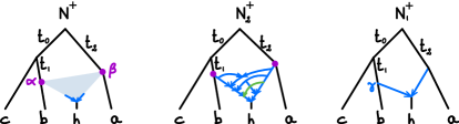
Figure 10: Example rooted networks that are not distinguishable from pairwise logDet distances. $N^{+}$ (left) shows the general structure of an ultrametric binary network on $\{a,b,c,h\}$ such that $N^{+}_{\{a,b,c\}}$ is the rooted tree $ab|c$, incident to the funnel of $h$ only once on its pendent edges to $a$ and to $b$. $N^{+}_{1}$ (right, outer-labeled planar utrametric level-1) and $N^{+}_{2}$ (middle) have this structure. $N^{+}_{2}$ is not outer-labeled planar, but would be if the green edge were removed. These networks have the same two rooted displayed tree topologies.

For such a network $N^{+}$, consider the rooted ultrametric level-1 network $N^{+}_{1}$ in Figure 10 (right) where $\gamma=\alpha$. Since no coalescent event can occur in the funnel of $h$ on $N^{+}$ or $N^{+}_{1}$, these networks yield the same metric gene tree distribution and therefore same pairwise logDet distances under the DT, NMSCcom, and NMSCind models with constant mutation rate. Analogously to the example given for the limits of identifiability under CFs, these examples generalize to networks with larger blobs.

In fact under the standard models we consider, the networks of this section are nonidentifiable from any sequence data if only one individual is sampled per taxon. Indeed, from such sequences, we can at best identify metric gene trees, but these do not distinguish the networks [20]. While data from multiple samples from the hybrid taxon $h$ may give additional information, it remains unclear what structure within the blob may then be identified (but see [26] for an example of two non-outer-labeled planar rooted networks with identical displayed trees, distinguishable using 2 samples from the hybrid taxon).

Appendix A Extension to non-binary networks

We now prove an extension of Lemma 5.1. For binary networks, there are only 2 cases in Lemma 5.1: a network has either a cut edge separating $ab$ from $cd$ up to relabeling of leaves (Case 1) or has a 4-blob (Case 2). When relaxing the binary assumption, Case 1 extends to networks with a blob that admits $ab$ and/or $cd$ as a taxon block. Case 2 remains unchanged, but the network may also display the unresolved star tree. All other networks (Case 3) display the star tree only.

Lemma A.1.

Let $N$ be a network on $\{a,b,c,d\}$. Then one of the following holds:

1. $N$ has a 2- or 3-blob with at least one 2-taxon block, say $ab$, and displays the quartet $ab|cd$ and no other resolved quartet. If $N$ is also outer-labeled planar, it is congruent with circular orders $(a,b,c,d)$ and $(a,b,d,c)$.

2. $N$ has a 4-blob, and displays at least 2 resolved quartets. If the 4-blob of $N$ is also outer-labeled planar, with unique circular order $(a,b,c,d)$, then $N$ displays exactly 2 resolved quartets, $ab|cd$ and $ad|bc$.

3. $N$ has a central node whose deletion leaves the taxa in 4 distinct connected components, and displays only the unresolved star quartet.

Simple examples show that $N$ may or may not also display the unresolved star quartet if it has no 2-blob with a 2-taxon group, regardless of whether it has a 3- or 4-blob.

In the proof below, we call a network’s blob pendent to taxon $x$ if it is a 2-blob with taxon blocks $x$ versus all the other taxa. The pendent blob chain to taxon $x$ is the subnetwork consisting of all nodes and edges in blobs pendent to $x$.

Proof.

We first prove that the blob conditions of Cases 1, 2 and 3 are exhaustive. On 4 taxa any 3-blob must have a taxon block of size 2, so if the conditions of Case 1 and 2 are not met, then $N$ does not have any 3-blob, 4-blob, or 2-blob with a taxon block of size 2. Then we claim that $N$ has a central node $z$.

To see this, consider the block-cut tree $G$ of $N$, with node set comprised of $N$’s blobs and cut nodes, and edges joining blobs and cut nodes adjacent in $N$. $G$ is a tree [10, Lemma 3.1.4]. Pendent cut edges in $N$ form the leaves of $G$. An $m$-blob in $N$ corresponds to a degree-$m$ vertex in $G$. In the absence of degree-3 blobs in $N$, a degree-3 vertex in $G$ corresponds to a cut node in $N$ incident to three 2-blobs, one of which must have a taxon block of size 2. Therefore $G$ has no degree-3 vertex, and has a degree-4 vertex corresponding to a central cut node $z$ in $N$. Then $N$ consists of 4 pendent blob chains adjacent to $z$, one to each taxon; and all displayed trees are stars with $z$ as a central node. If $N$ is outer-labeled planar, that is, if its pendent chains are planar, then $N$ is easily seen to be congruent with all 3 circular orders.

In Case 1, assume that $N$ has a blob $B$ with $ab$ as one taxon block. Within a tree $T$ displayed in $N$, the edge(s) retained from $B$ must then map to edge(s) in $T$, one of which must be a cut edge separating $ab$ from the other 2 taxa, as claimed. To show that such an outer-labeled planar $N$ is congruent with the orders $(a,b,c,d)$ and $(a,b,d,c)$, we build outer-labeled planar networks displaying $N$, each with a 4-blob and these orders. Since a pendent edge can be directed towards the leaf, we build these from $N$ by adding a hybrid edge from either of the edges incident to $c$ or $d$ to the edge incident to $a$, after rotating part of the planar network about the blob’s articulation node for $ab$ if necessary.

For Case 2, consider $N$ with a 4-blob $B$. Let $v$ be a lowest hybrid node in $B$. We may assume that removing any parent edge of $v$ (and then edges no longer on up-down paths between taxa) gives a subnetwork without a 4-blob. Otherwise, we remove such edges iteratively until we cannot do so while retaining a 4-blob, and observe that any quartet displayed in the modified network is also displayed in $N$. Let $d$ be the taxon below $v$; $e_{1}=(v_{1},v),\ldots,e_{k}=(v_{k},v)$ the parent edges of $v$; and $N_{j}$ the network obtained from $N$ by removing $e_{j}$ and nodes and edges no longer an up-down paths between taxa, so as to prune unlabeled leaves. We will prove that at least two of $N_{1},\ldots,N_{k}$ fall under Case 1 for distinct quartets. For the sake of contradiction, assume that for all $j$, $N_{j}$ falls under Case 1 for quartet $ab|cd$ (and so has a blob with taxon group $ab$ or $cd$) or under Case 3 (and has a central node whose deletion separates all taxa).

Consider the subnetwork $\widetilde{N}$ induced by $a,b,c$. Then $\widetilde{N}$ is a subgraph of $N_{j}$ for all $j$. If $\widetilde{N}$ has a central node whose deletion separates all 3 taxa $a,b,c$, call this node $z$. Otherwise, $\widetilde{N}$ must have a 3-blob (corresponding to the degree-3 node in $\widetilde{N}$’s block-cut tree), and let $z$ be its articulation node leading to $c$. In both cases, $z$ belongs to the pendent blob chain to $c$ in $\widetilde{N}$, and separates this blob chain from the subnetwork of $\widetilde{N}$ (and of $N$) induced by $a,b$.

Since a blob $\widetilde{B}$ of $\widetilde{N}$ is biconnected, any blob $B$ of $N_{j}$ either contains $\widetilde{B}$, or shares no edge with $\widetilde{B}$. If $N_{j}$ has a blob $B$ with taxon block $ab$, then $B$ may only contain blobs from $\widetilde{N}$ that are pendent to $c$, therefore $N_{j}$ is formed from $\widetilde{N}$ by attaching a subgraph to the pendent blob chain to $c$. If $N_{j}$ has no blob with taxon block $ab$ but a blob $B$ with taxon block $cd$, then $B$ is on $\widetilde{N}$, and $N_{j}$ is formed from $\widetilde{N}$ by attaching a pendent blob chain to $d$ at $z$.

Thus in either case, $N_{j}$ results from attaching a subgraph to $\widetilde{N}$ only along the pendent blob chain to $c$. Therefore $z$ disconnects the subnetwork induced by $a,b$ from the subnetwork induced by $c,d$ in the full network $N$, and $N$ cannot have a 4-blob — a contradiction.

The first claim of Case 2 follows easily, having established Case 1 and that at least two of $N_{1},\ldots,N_{k}$ fall under Case 1 for distinct quartets. If $N$ is outer-labeled planar, by Corollary 4.2 it has a unique circular order, say $(a,b,c,d)$. Then by Lemma 4.3, the displayed quartets can only be $ab|cd$ and $ad|bc$. ∎

References

- ABGLR [24] Elizabeth S. Allman, Hector Baños, Marina Garrote-Lopez, and John A. Rhodes. Identifiability of level-1 species networks from gene tree quartets. arXiv, 2024.
- ABMR [23] Elizabeth S. Allman, Hector Baños, Jonathan D. Mitchell, and John A. Rhodes. The tree of blobs of a species network: Identifiability under the coalescent. Journal of Mathematical Biology, 86(1):10, 2023.
- ABnR [22] Elizabeth S. Allman, Hector Baños, and John A. Rhodes. Identifiability of species network topologies from genomic sequences using the logDet distance. Journal of Mathematical Biology, 84:35, 2022.
- ABR [19] E.S. Allman, H. Baños, and J.A. Rhodes. NANUQ: A method for inferring species networks from gene trees under the coalescent model. Algorithms Mol. Biol., 14(24):1–25, 2019.
- ADR [11] E.S. Allman, J.H. Degnan, and J.A. Rhodes. Identifying the rooted species tree from the distribution of unrooted gene trees under the coalescent. Journal of Mathematical Biology, 62(6):833–862, 2011.
- AFA+ [23] Cécile Ané, John Fogg, Elizabeth S. Allman, Hector Baños, and John A. Rhodes. Anomalous networks under the multispecies coalescent: theory and prevalence. bioRxiv, 2023.
- ALR [19] E.S. Allman, C. Long, and J.A. Rhodes. Species tree inference from genomic sequences using the log-det distance. SIAM J. Appl. Algebra Geometry, 3:107–127, 2019.
- Ard [21] Muhammad Ardiyansyah. Distinguishing level-2 phylogenetic networks using phylogenetic invariants. arXiv:2104.12479, 2021.
- Bn [19] H. Baños. Identifying species network features from gene tree quartets. Bulletin of Mathematical Biology, 81:494–534, 2019.
- Die [17] R. Diestel. Graph Theory, volume 173 of Graduate Texts in Mathematics. Springer Verlag, 5th edition, 2017.
- DYN [12] J. Degnan, Y. Yu, and L. Nakhleh. The probability of a gene tree topology within a phylogenetic network with applications to hybridization detection. PLoS Genet, 8(4):271–282, 2012.
- FAA [23] John Fogg, Elizabeth S Allman, and Cécile Ané. PhyloCoalSimulations: A simulator for network multispecies coalescent models, including a new extension for the inheritance of gene flow. Systematic Biology, in press, 2023.
- GBBS [07] D. Gusfield, V. Bansal, V. Bafna, and Y.S. Song. A decomposition theory for phylogenetic networks and incompatible characters. Journal of Computational Biology, 14(10):1247–1272, 2007.
- GBP [12] Philippe Gambette, Vincent Berry, and Christophe Paul. Quartets and unrooted phylogenetic networks. Journal of Bioinformatics and Computational Biology, 10(4):1250004, 2012.
- GGK [11] David Gerard, H. Lisle Gibbs, and Laura Kubatko. Estimating hybridization in the presence of coalescence using phylogenetic intraspecific sampling. BMC Evolutionary Biology, 11(1), 2011.
- GHS [17] P. Gambette, K.T. Huber, and G.E. Scholz. Uprooted phylogenetic networks. Bulletin of Mathematical Biology, 79(9):2022–2048, 2017.
- GvIJ+ [21] E. Gross, L. van Iersel, R. Janssen, M. Jones, C. Long, and Y. Murakami. Distinguishing level-1 phylogenetic networks on the basis of data generated by Markov processes. Journal of Mathematical Biology, 83:32, 2021.
- HRS [10] Daniel H. Huson, Regula Rupp, and Celine Scornavacca. Phylogenetic Networks. Cambridge University Press, Cambridge, 2010.
- JY [21] Xiyun Jiao and Ziheng Yang. Defining species when there is gene flow. Systematic Biology, 70(1):108–119, 2021.
- PS [15] Fabio Pardi and Celine Scornavacca. Reconstructible phylogenetic networks: Do not distinguish the indistinguishable. PLOS Computational Biology, 11(4):e1004135, 2015.
- Rho [20] J.A. Rhodes. Topological metrizations of trees, and new quartet methods of tree inference. IEEE/ACM Trans. Comput. Biol. Bioinform., 17(6):2107–2118, 2020.
- SLA [16] C. Solís-Lemus and C. Ané. Inferring Phylogenetic Networks with Maximum Pseudolikelihood under Incomplete Lineage Sorting. PLoS Genetics, 12(3):e1005896, 2016.
- SS [05] C. Semple and M. Steel. Phylogenetics. Oxford University Press, 2005.
- Ste [94] M.A. Steel. Recovering a tree from the leaf colourations it generates under a Markov model. Applied Mathematics Letters, 7(2):19–24, 1994.
- XA [23] Jingcheng Xu and Cécile Ané. Identifiability of local and global features of phylogenetic networks from average distances. Journal of Mathematical Biology, 86(1):12, 2023.
- ZD [17] Sha Zhu and James H. Degnan. Displayed trees do not determine distinguishability under the network multispecies coalescent. Systematic Biology, 66(2):283–298, 2017.