On properties of the sets of positively curved Riemannian metrics on generalized Wallach spaces
N. A. Abiev
N. A. Abiev
Institute of Mathematics NAS KR, Bishkek, prospect Chui, 265a, 720071, Kyrgyz Republic
abievn@mail.ru
Abstract.
Sets related to positively curved invariant Riemannian metrics on generalized Wallach spaces
are considered.
The problem arises in studying of the evolution of such metrics under the normalized Ricci flow equation.
For Riemannian metrics of the Wallach spaces
, and
which admit positive sectional curvature and belong to a given
invariant surface of the normalized Ricci flow
we established that they form a set bounded by three connected and pairwise disjoint
regular space curves such that
each of them approaches two others asymptotically at infinity.
Analogously, we proved that for all generalized Wallach spaces
the set of Riemannian metrics
which belong to and admit positive Ricci curvature
is bounded by three curves each consisting of two connected components
as regular curves. Intersections and asymptotical behaviors of these
components were studied as well.
Key words and phrases: Wallach space, generalized Wallach space,
Riemannian metric, normalized Ricci flow, sectional curvature, Ricci curvature, invariant set.
The paper is devoted to the study of structural properties of two important sets
responsible for positivity of the sectional and the Ricci curvatures
of invariant Riemannian metrics on the Wallach spaces and generalized Wallach spaces.
The Wallach spaces
(1)
are well-known and admit invariant Riemannian metrics of positive sectional curvature (see [24] for details).
As for generalized Wallach space, firstly, recall its definition and basic properties
(see [18, 20]).
Let be a homogeneous almost effective compact space with a (compact) semisimple connected Lie group and its closed subgroup . Denote by and the corresponding Lie algebras of and .
Then is a corresponding Lie bracket
of whereas is
the Killing form of . Note that
is a bi-invariant inner product on .
In this way invariant Riemannian metrics on can be identified with -invariant inner products on the
orthogonal complement of in with respect to .
Compact homogeneous spaces whose isotropy representation admits a decomposition into a direct sum
of three
-invariant irreducible modules
, and
satisfying
for each
were called three-locally-symmetric spaces according to [17]
or generalized Wallach spaces in the terminology of [20].
The main characteristic of these spaces is that every generalized Wallach space can be described by a triple of real parameters , ,
where and is some important positive constant
(see [17, 18] for details).
It should be also noted that not every triple corresponds to some generalized Wallach spaces.
An interesting fact is the fact that the Wallach spaces (1)
are partial cases of generalized Wallach spaces
with , and respectively (see [8]).
As noted above for a fixed bi-invariant inner product
on the Lie algebra of the Lie group ,
any -invariant Riemannian metric on can be determined by an -invariant inner product
(2)
where are positive real numbers
(a detailed exposition can be found in [17, 18, 19, 20] and references therein).
In [18] the explicit expressions
and
were derived
for the Ricci tensor and
the scalar curvature of the metric (2)
on generalized Wallach spaces,
where
(3)
are the principal Ricci curvatures,
.
Knowing and
allowed us to initiate in [6]
the study of the normalized Ricci flow equation
(4)
introduced by R. Hamilton in [16]
on generalized Wallach spaces.
Since then studies related to this topic
were continued in [1, 3, 7, 22]
concerning
classifications of singular (equilibria) points of (4)
being Einstein metrics
and their bifurcations.
The authors of [2, 10, 11] studied an interesting and quite complicated
surface of bifurcations
of (4)
defined by a symmetric polynomial equation in three variables of degree .
In the sequel authors of [4, 8] considered
the evolution of positively curved Riemannian metrics under the influence
of (5) on an interesting
class of generalized Wallach spaces with coincided parameters
generalizing some results of [14, 15].
In this case (4) can be reduced to the following system
of three autonomous ordinary differential equations (see [8]):
(5)
with .
A relevant information on homogeneous spaces admitting positive sectional or (and) positive Ricci curvatures can be found in
[9, 12, 13, 24, 25, 26, 27] and references therein.
In [8] it was proved that (4) deforms
all generic metrics with positive sectional curvature into metrics with mixed sectional curvature on each Wallach space in (1)
(Theorem 1 in [8]) and all generic metrics with positive Ricci curvature will be deformed into metrics with mixed Ricci curvature for and (see Theorem 2 in [8]), where given a metric is said to be generic if for .
According to Theorems 3 and 4 in [8] and Theorem 3 in [4]
positiveness of the Ricci curvature will be preserved
for all metrics at
and for a special kind of metrics
satisfying at
(the equalities correspond to Kähler metrics),
whereas all positively curved metrics will be deformed into metrics with mixed Ricci curvature
if .
In [4, 8] we used the description
(6)
of the set of Riemannian metrics with positive sectional curvature on the Wallach spaces (1) given in [23]
and the description
(7)
of the set of Riemannian metrics of positive Ricci curvature
on generalized Wallach spaces in the case
given in [18].
According to [23] the system of inequalities describes the set
of Riemannian metrics of positive sectional curvature on the Wallach spaces (1)
and, analogously, solutions of the system of inequalities
represents the set of all Riemannian metrics of positive Ricci curvature
on every generalized Wallach spaces with as follows from (3).
In [4, 8] we relied on Maple evaluations and our visual observations concerning
structural properties of surfaces and curves obtained from (6) and (7),
but justifications of those properties were not included into the text of the papers.
Filling these gaps we initiated in [5].
The present paper continues that idea.
For denote by and the surfaces
in
defined by the equations and
respectively and introduce space curves ,
and sets , .
The main result of this paper is contained in the following two theorems.
Theorem 1.
The following assertions hold
for all indices with :
(1)
For each Wallach space in (1) the set
of invariant Riemannian metrics (2) which belong to the invariant set of the system (5) and
admit positive sectional curvature
is bounded by the pairwise disjoint regular space curves
, and in such that each is connected and
can be parameterized as the following
where
and ;
(2)
Every invariant curve of the system (5)
given by the equations , , ,
intersects the only border curve at the unique
point with coordinates ,
approaching at infinity the other two curves and
as close as we like, where .
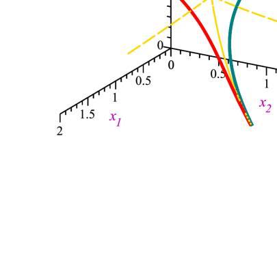
The results of Theorem 1
are illustrated in the left panel of Figure 1,
where the curves , and are depicted respectively
in red, teal and blue colors,
the invariant curves are all yellow colored.
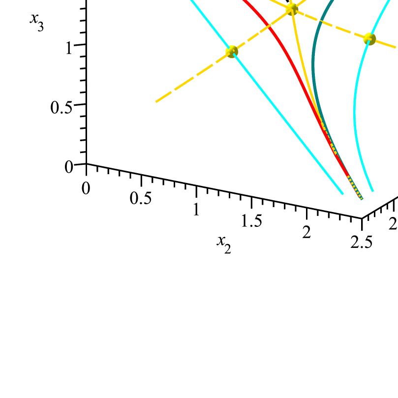
Figure 1. The left panel: the curves ; The right panel: the curves , and singular points corresponding to .
Theorem 2.
The following assertions hold
for all indices with :
(1)
For every generalized Wallach space with
the set
of invariant Riemannian metrics (2) which belong to the invariant set of the system (5) and
admit positive Ricci curvature
is bounded by the space curves
, and in such that
each consists of two regular connected components and
parameterized by equations
(8)
and
(9)
respectively, where
and .
(2)
Every pair of the curves and admits a unique common point with coordinates
,
which belong to the components and ;
In addition, every invariant curve of the system (5)
meets the components and of and exactly at the point
approaching their another components and
at infinity as close as we like.
(3)
For every
all singular (equilibria) points
of the system (5)
belong to the set .
(4)
Kähler metrics of generalized Wallach spaces with form in separatrices of saddles of (5) which can be defined by parametric equations
(10)
where and .
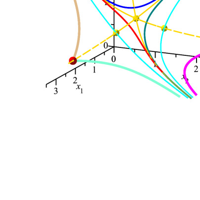
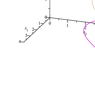
The results of Theorem 2
are illustrated in the right panel of Figure 1
for the case ,
where the curves , and are depicted respectively
in magenta, aquamarine and burlywood colors,
the curves , and are depicted by cyan colored curves
and yellow colored points correspond to singular points of (5).
It should be noted that we will consider only Riemannian metrics
satisfying the unit volume condition (see [6, 8]),
and denote by the surface defined by equation with
.
In general, surfaces , where ,
play the significant role for study (5)
on generalized Wallach spaces.
It is known that any set determined by the
equation
is invariant under (5), moreover is its first integral.
Surfaces will also be unstable (or stable) manifolds of (5) and contain leading directions of motions of its trajectories (see [5]).
Since the right hand sides of (5)
are all homogeneous, namely
for any ,
we can pass to a new differential system of the same form as the original one, but
with .
Actually this is reachable by replacings and .
Therefore without loss of generality
we assume that the invariant surface is given by .
1. Auxiliary results
Observe that the expressions for and in (6) and (7) are symmetric under the permutations .
Therefore it suffices to consider representatives only at fixed ,
where .
For each Wallach space in (1)
the set of Riemannian metrics (2) with positive sectional curvature is bounded by the pairwise disjoint conic surfaces
, and .
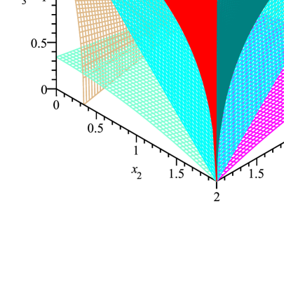
The cones , and are depicted
in the left panel of Figure 2 in red, teal and blue colors respectively.
Actually Lemma 1 was proved in [5].
Here we bring the sketch of its proof for convenience of the readers.
The equation defines two connected components
and
of the cone .
Since the first of them gives for all
then is equivalent to
meaning that is bounded by the plane and the positive part
of the cone . By symmetry we have the same
for and .
Consider the pair . The equations and
defining the surfaces and
can admit only the following two family of common solutions ,
and , . But we need in positive solutions only.
Hence for all positive .
By symmetry the same assertions hold for the pairs and .
Figure 2. The left panel: the cones ,
and the planes for ;
The right panel: crossing and by .
Lemma 2.
For every generalized Wallach space with the set
is bounded by the conic surfaces
, and .
Each pair and has intersections along two different straight lines , and , , where .
The cones , and are depicted
in the left panel of Figure 2 in magenta, aquamarine and burlywood colors respectively.
Proof of Lemma 2.
Consider the surface .
Since is symmetric with respect to and
it can be considered as a quadratic polynomial in
without loss of generality.
Then
if and
if or ,
where
(11)
Depending on the sign of
the inequality admits the positive solution
if and any can satisfy if .
This means that besides the planes , and the set
is bounded by two disjoint connected components
and of the surface
defined by the same equation
but on different domains
and
respectively.
Due to symmetry the same properties hold for
the surfaces and as well.
Thus .
By the same reason of symmetry it suffices to analyze only.
Assume that some triple satisfies both of
and .
Then and imply
and .
In what follows that the system of equations and
can admit only the following two different families of one-parametric solutions , and
(12)
with parameters .
2. Proofs of the main results
Proof of Theorem 1.The curves are pairwise disjoint and
bound the set because so are
the corresponding cones
and
according to Lemma 1.
Parameterizations of the curves , and .
Due to symmetry fix any unordered triple .
Putting in
we obtain the following polynomial equation of degree in two variables and :
After then substituting , into the obtained equation and solving it with respect to we can get a parametric
representation of the curve given in (1).
It is expected its two different roots
, , ,
but the second of these roots taken with the minus sign gives only negative values
of and .
Denote .
Note also that and
.
This yields
,
and , .
Connectedness of the curves , and .
Note that .
Hence assigning we define on a continuous function
Therefore in the standard topology of the set (curve)
must be connected as a continuous image of the connected set
under a function
with continuous coordinate components such that
, and .
Smoothness of the curves , and
can be proved using (1).
But we prefer another way. Due to symmetry it suffices
to prove smoothness of the curve .
Since and are smooth (regular) surfaces
it remains to show that their intersection is transversal, in other words
their gradient vectors
and
are linearly independent
along , where
for .
Due to symmetry fix any and suppose by contrary that for some real .
This means that the equalities
hold for .
Then for and we obtain
equalities
equivalent to which is impossible
for .
Actually we proved the more strong fact that the normal vectors
and are linearly independent
not only along , but everywhere where the surfaces
and are defined excepting points
with non positive or coincided components.
Due to symmetry it suffices to take the invariant curve of (4)
defined as , , .
Consider the curve .
The question is will cross the curve or not.
It suffices to answer this question for and the surface
because existing of a point in such that
implies and hence .
Thus substituting , into the equation of
we obtain the equation
which admits the single root providing the unique common point , of with .
Consider now any curve such that .
Then we obtain an incompatible system
of equations , and because of
.
Moreover, asymptotically tends to as according to
.
The same result holds for by symmetry in the equation of .
Theorem 1 is proved.
Proof of Theorem 2.
Clearly directly follows
from proved in
Lemma 2.
Intersecting both of the connected components
and of the cone
the surface forms components and
of the curve such that and
.
Smoothness of the components of , and .
Consider the curve .
We claim that the
gradient vectors
and
of the surfaces and are linearly independent
for all positive such that ,
where
for .
Indeed supposing , where is a nonzero real number,
we obtain immediately an unreachable equality .
In what follows that each component and
of the curve is a smooth curve as a transversal intersection of two smooth surfaces.
Connectedness of the components of .
The variable can be eliminated from the system of equations and
to obtain the equation
of the projection of the curve
onto the coordinate plane .
By the same way as in Theorem 1
substituting , into the last equation
and solving it with respect to we obtain a parametric
equation
of the curve ,
where
The function is
well defined, continuous and positive valued for or ,
where and are given in (11), .
It follows then the components and of are
respectively continuous images of the connected sets
and under a vector-function with
coordinates , and .
Therefore and are connected too.
Note that the components and
are symmetric under the permutation .
Therefore we can parameterize them on the same interval
but using different formulas
(8) and (9) respectively.
For simplicity we choose the interval .
Intersections of , and .
Consider the pair and .
By Lemma 2 the surfaces and meet each other along
the straight line , (see (12)).
This line intersects the surface
at a unique point . Indeed substituting
, into we get the unique value
.
This yields coordinates of .
Note that (the point in the right panel of Figure 2)
is also the only intersection point of the curves and
(their components and ).
Now a value of at which belongs to
can be found from the parametric representation
of .
The condition implies an equation
which has the single root for all .
Therefore the curve passes through at only.
It should be noted that the curves and leave extra pieces after crossing each other.
In principle, we can preserve them, but
it is advisable to remove them for greater clarity of pictures.
Analyzing the values of limits
and
we conclude that the tail corresponds to values .
Therefore the original interval of parametrization can be reduced
to the interval shown in the text of Theorem 2.
By symmetry the analysis of the pairs and
(points in teal and red color in the right panel of Figure 1)
will be the same using permutations of the indices .
For example, the equations
, and
define another connected component of the curve (which intersects )
on the same interval . Then coordinates
of the point
(in fact )
can be obtained at the same boundary value (the point in the right panel of Figure 2).
Analogously at we get the part of .
Without loss of generality consider the invariant curve .
As noted in Theorem 1
it suffices to consider the surfaces
instead of the corresponding curves .
The curve crosses both of the curves and
(the components and )
exactly at their common point
because substituting , into and
yields the equations
which admit a single root corresponding to .
Therefore .
At the same time
approximates both of and (their components and ) at infinity.
Indeed
For the curve we have
under the same substitutions.
Therefore never cross , moreover, .
As it follows from [6, 17]
the system of algebraic equations
has the following four families of one-parametric solutions
for every :
(13)
where
(14)
At these families merge to the unique family .
Substituting and into
the expressions (7) for and we obtain
because .
Obviously,
at .
Therefore the straight lines (13) lye in the set
for all . They cross the invariant surface
at the points (see also [5])
being the singular points of the system (5) on , where
(at the unique singular point is obtained
according to (14)).
Thus we conclude that for every
and .
According to [4, 6, 7]
the curves , and are
separatrices of the unique saddle point (of the linear zero type)
of the system (5) if .
For
the points are all hyperbolic type saddles
and is a stable (respectively unstable) hyperbolic node
if (respectively ).
Additionally, each invariant curve is one of two
separatrices of the saddle (see [5]).
At we have an opportunity
to find analytically the second separatrice of each
different from , where .
Indeed it is easy to see that coordinates of
satisfy the system of equations
(15)
where
represents Kähler metrics
on a given generalized Wallach space with ,
(see also [8]).
Therefore each saddle
belongs to a curve obtained as an intersection of the invariant surface with the plane
(the curves are depicted in the right panel of Figure 1 in cyan color for all indices ).
Repeating similar procedures as in the case of the curves and
we can obtain parametric equations (10)
of the curves .
Clearly, for .
We claim that each of is also an invariant curve of the differential system (5).
To show it consider the case only due to symmetry.
Substitute the parametric representation
, , of the curve
into and in (5), where
, .
Then
The value providing gives a stationary trajectory,
namely it is the singular point itself.
Thus assume .
The identities
imply that
is a trajectory of (5)
for and .
Moreover, passes through the singular point as noted above.
This means that is a separatrice of .
Invariancy of the curves and respectively
passing through and
can be proved by the same way.
Theorem 2 is proved.
Remark 1.
As it was noted in the proof of Theorem 2
the equations (8) define for
the same curve as (9) for .
In the case the tail removing procedure leads
to the equation
equivalent to .
Its first root corresponds to the point
and the second root gives the point .
Obviously for all .
Therefore, in principle, both components of each curve can be parameterized
by one formula, say (8), but using the different intervals and .
Remark 2.
We proved that all singular points
and
of the normalized Ricci flow on generalized Wallach spaces with
belong to the set
of metrics with positive Ricci curvature.
Unfortunately a similar assertion does not hold for the
set . Lemma 3 in [5] shows that there exists a critical value such that
only if and the
boundary cases () hold if .
The only generalized Wallach spaces which admit metrics with
positive sectional curvature are the Wallach spaces (1) which satisfy the condition .
Remark 3.
The case is original,
where Kähler metrics provide separatrices of saddles as it illustrated
in Figure 1.
For it is a difficult problem to find
similar separatrices analytically.
Knowing all separatrices allows to
predict the dynamics of the Ricci flow in more detail.
To demonstrate the main idea consider
an arbitrarily chosen singular point in the case , say
(the Kähler-Einstein metric) and observe that the curve defined by the equations and coincides with the unstable manifold
of as it was shown in [5].
The stable manifold of
is .
It is clear now that controlling by and trajectories of (5) never can leave the domain bounded by the curves (15).
This explains the fact proved in Theorem 4 in [8]
that Riemannian metrics (2)
on generalized Wallach spaces with (on the Wallach space in particularly)
preserve the positivity of their Ricci curvature for ().
In Figure 3 the separatrices and some trajectories
of (5) are depicted for illustrations.
Figure 3. The separatrices (in cyan color), (in yellow color) and trajectories of (5) (in black color).
3. Additional remarks
i) The well known fact that the positivity of the Ricci curvature
follows from the positivity of the sectional curvature
can be justified and illustrated via inclusion , where
is depicted in Figure 2 as a set bounded by three cones in red, teal and blue colors,
respectively is bounded by six conic surfaces in magenta, aquamarine and burlywood colors.
To establish for all
it suffices to show the inclusion .
We will follow this opportunity since trying to establish directly
leads to pairs of inequalities of the kind and
whose analysis is much more complicated than to deal with the system consisting of
one equation
and one inequality :
(16)
By symmetry fix any
and consider the component of the boundary of .
Every point of the cone belongs to some its generator line
, , , (see also [5]),
where
, .
Indeed generators satisfy the equation in (16)
and the inequality in (16)
takes the form
with
and
.
Obviously for all and .
Since has roots and
the inequality holds as well at .
Thus is equivalent to
, where
admits two different negative roots
and
for every .
It follows then (hence ) at independently on .
This means that for any point of
which is equivalent to .
Since was chosen arbitrarily we obtain
and hence with the obvious
consequence .
ii) There are useful asymptotical representations for practical aims.
For instance, at the expressions
are valid for coordinates of points of the curve defined
as a variety of solutions of the system
(17)
For tending to the curve
has a similar asymptotic
in accordance with the fact that and
approach the same invariant curve at infinity.
iii) Often it is easier to deal with a planar analysis of the dynamics of the normalized Ricci flow.
Choose the coordinate plane without loss of generality. Then the projection of the set of Riemannian metrics with positive sectional curvature
onto the plane
can be bounded by the following plane curves and defined implicitly
For example the equation of can be obtained eliminating in the system (17).
Analogously, boundary curves of the projection of the set of Ricci positive metrics onto the plane have equations
Projections of the Kähler metrics
, and will be defined by
, and respectively.
We recommend to compare the pictures demonstrated in this paper with planar pictures depicted in the right panels of Figures 3, 6 and 7 obtained in [8] in the coordinate plane .
The author is grateful to Prof. Yu. G. Nikonorov for helpful discussions.
References
[1]Abiev N.A. On classification of degenerate singular points of Ricci flows.
Bull. Karaganda Univ.-Math.
(2015), V. 79, No. 3, P. 3–11.
[2]Abiev N.A. On topological structure of some sets related to
the normalized Ricci flow on generalized Wallach spaces.
Vladikavkaz. Math. J. (2015), V. 17, No. 3, P. 5–13.
[3]Abiev N.A. Two-parametric bifurcations of singular points of
the normalized Ricci flow on generalized Wallach spaces.
AIP Conference Proceedings. (2015), V. 1676, 020053, P. 1–6.
[4]Abiev N. A.
On the evolution of invariant Riemannian metrics on one class
of generalized Wallach spaces under the influence of the normalized Ricci flow.
Matem. tr. (2017), V. 20, No. 1. P. 3–20 (Russian); English translation in: Siberian Adv. Math. (2017), V. 27, No. 4, P. 227–238.
[5]Abiev N. A.
On the dynamics of a three-dimensional differential system related to the normalized Ricci flow on generalized Wallach spaces, https://arxiv.org/abs/2312.09706 (Preprint).
[6]Abiev N. A., Arvanitoyeorgos A., Nikonorov Yu. G., Siasos P.
The dynamics of the Ricci flow on generalized Wallach spaces.
Diff. Geom. Appl. (2014), V. 35, Supplement, P. 26–43.
[7]Abiev N. A., Arvanitoyeorgos A., Nikonorov Yu. G., Siasos P.
The Ricci flow on some generalized Wallach spaces. In: V. Rovenski, P. Walczak (eds.).
Geometry and its Applications. Springer Proceedings in Mathematics & Statistics, V. 72,
Switzerland: Springer, 2014, VIII+243 p., P. 3–37.
[8]Abiev N. A., Nikonorov Yu. G.
The evolution of positively curved invariant Riemannian metrics on the Wallach spaces under the Ricci flow. Ann. Glob. Anal. Geom. (2016), V. 50, No. 1. P. 65–84.
[9]Aloff S., Wallach N.
An infinite family of 7–manifolds admitting positively curved Riemannian structures. (1975),
Bull. Amer. Math. Soc., 81, 93–97.
[10]Batkhin A. B., Bruno A. D. Investigation of a real
algebraic surface. Program. Comput. Software (2015),
V. 41, No. 2. P. 74–83.
[11]Batkhin A. B. A real variety with boundary
and its global parameterization. Program. Comput. Software (2017),
V. 43, No. 2. P. 75–83.
[12]Bérard Bergery L.
Les variétés riemanniennes homogènes simplement connexes de dimension impaire
à courbure strictement positive. J. Math. Pures Appl. (1976), V. 55, P. 47–68.
[13]Berger M. Les variétés riemanniennes homogènes normales simplement connexes à courbure strictment positive.
Ann. Scuola Norm. Sup. Pisa (1961), V. 15, P. 191–240.
[14]Böhm C., Wilking B.
Nonnegatively curved manifolds with finite fundamental groups admit metrics with positive Ricci curvature. GAFA Geom. Func. Anal. (2007), V. 17, P. 665–681.
[15]Cheung Man-Wai, Wallach N. R.
Ricci flow and curvature on the variety of flags on the two dimensional projective space over the complexes, quaternions and octonions. Proc. Amer. Math. Soc. (2015), V. 143, No. 1, P. 369–378.
[16]Hamilton R. S. Three-manifolds with positive Ricci curvature.
J. Diff. Geom. (1982), V. 17, P. 255–306.
[17]Lomshakov A. M., Nikonorov Yu. G., Firsov E. V. Invariant
Einstein metrics on three-locally-symmetric spaces. Matem. tr. (2003), V. 6, No. 2.P. 80–101 (Russian); English translation in: Siberian Adv. Math. (2004), V. 14, No. 3, P. 43–62.
[18]Nikonorov Yu. G. On a class of homogeneous compact
Einstein manifolds. Sibirsk. Mat. Zh. (2000), V. 41, No. 1, P. 200–205 (Russian);
English translation in: Siberian Math. J. (2000), V. 41, No. 1, P. 168–172.
[19]Nikonorov Yu. G. Classification of generalized Wallach spaces.
Geom. Dedicata (2016), V. 181, No 1. P. 193–212; correction: Geom. Dedicata (2021), V. 214,
No 1. P. 849–851.
[20]Nikonorov Yu. G., Rodionov E. D., Slavskii V. V.
Geometry of homogeneous Riemannian manifolds. Journal of Mathematical Sciences (New York) (2007), V. 146, No. 7, P. 6313–6390.
[21]Rodionov E. D.
Einstein metrics on even-dimensional homogeneous spaces admitting a homogeneous Riemannian metric of positive sectional curvature, Sibirsk. Mat. Zh. (1991), V. 32, No. 3, P.126–131 (Russian); English translation in: Siberian Math. J. (1991), V. 32, No. 3, P. 455–459.
[22]Statha M.
Ricci flow on certain homogeneous spaces,
Ann. Global Anal. Geom. (2022), V. 62, No. 1, P.93–127.
[23]Valiev F. M.
Precise estimates for the sectional curvature of homogeneous Riemannian metrics on Wallach spaces.
Sib. Mat. Zh. (1979), V. 20, P. 248–262 (Russian);
English translation in: Siberian Math. J. (1979), V. 20, P. 176–187.
[24]Wallach N. Compact homogeneous Riemannian manifolds with
strictly positive curvature. Annals of Mathematics, Second Series. (1972), V. 96, No.2, P. 277–295.
[25]Wilking B.
The normal homogeneous space has positive sectional curvature.
Proc. Am. Math. Soc. (1999), V. 127, No. 4, P. 1191–1194.
[26]Wilking B., Ziller W.
Revisiting homogeneous spaces with positive curvature.
Journal Reine Angewandte Math. (2018), V. 738, P. 313–328.
[27]Xu M., Wolf J. A. and a positive curvature problem.
Differ. Geom. Appl. (2015), V. 42, P. 115–124.