A Fast Algorithm to Simulate Nonlinear Resistive Networks

Abstract

In the quest for energy-efficient artificial intelligence systems, resistor networks are attracting interest as an alternative to conventional GPU-based neural networks. These networks leverage the physics of electrical circuits for inference and can be optimized with local training techniques such as equilibrium propagation. Despite their potential advantage in terms of power consumption, the challenge of efficiently simulating these resistor networks has been a significant bottleneck to assess their scalability, with current methods either being limited to linear networks or relying on realistic, yet slow circuit simulators like SPICE. Assuming ideal circuit elements, we introduce a novel approach for the simulation of nonlinear resistive networks, which we frame as a quadratic programming problem with linear inequality constraints, and which we solve using a fast, exact coordinate descent algorithm. Our simulation methodology significantly outperforms existing SPICE-based simulations, enabling the training of networks up to 325 times larger at speeds 150 times faster, resulting in a 50,000-fold improvement in the ratio of network size to epoch duration. Our approach, adaptable to other electrical components, can foster more rapid progress in the simulations of nonlinear electrical networks.

1 Introduction

In order to reduce the energy consumption of artificial intelligence (AI), neuromorphic platforms based on analog physics and algorithms for such platforms are being explored as alternatives to GPU-based neural networks (Marković et al., 2020; Dillavou et al., 2022; Wright et al., 2022; Lopez-Pastor & Marquardt, 2023; Stern & Murugan, 2023; Scellier, 2021). In particular, nonlinear resistive networks have recently sparked some interest (Kendall et al., 2020; Dillavou et al., 2022, 2023; Wycoff et al., 2022; Anisetti et al., 2022; Stern et al., 2022, 2023; Kiraz et al., 2022; Watfa et al., 2023; Oh et al., 2023). Central to these networks are variable resistors (e.g. memristors) which act as trainable weights, coupled with diodes that introduce nonlinearities, as well as voltage and current sources for input signals. The conductances of these variable resistors can be adjusted, allowing the network to be trained to achieve specific computational tasks. Notably, like traditional neural networks, nonlinear resistive networks have two essential computational properties: they are universal function approximators (Scellier & Mishra, 2023) and they can be trained by gradient descent (Kendall et al., 2020; Anisetti et al., 2022). Unlike GPU-based neural networks, however, they leverage the laws of electrical circuits - such as Kirchhoff’s laws and Ohm’s law - to perform inference and gradient computation. Furthermore, the learning rules governing conductance changes are local. These features make nonlinear resistive networks good candidates as power-efficient self-learning hardware, with recent experiments on memristive networks suggesting a potential staggering 10,000x gain in energy efficiency compared to neural networks trained on GPUs (Yi et al., 2023). Small-scale self-learning variable resistor networks have been built and succesfully trained on datasets such as Iris (Dillavou et al., 2022, 2023), validating the soundness of the approach.

Simulations of larger nonlinear resistive networks on tasks such as MNIST (Kendall et al., 2020) and Fashion-MNIST (Watfa et al., 2023) further underscore their potential. These works and others (Kiraz et al., 2022; Oh et al., 2023) performed the simulations using the general-purpose SPICE circuit simulator (Keiter, 2014; Vogt et al., 2020). However, these efforts have been hampered by the slowness of SPICE, which is not specifically conceived to perform efficient simulations of resistive networks used for machine learning applications. To illustrate, Kendall et al. (2020) employed SPICE to simulate the training on MNIST of a one-hidden-layer network comprising 100 hidden nodes, a process which took one week for only ten epochs of training. Due to a scarcity of methods and algorithms for nonlinear resistive network simulations, another line of works resort to linear networks (Stern et al., 2022, 2023; Wycoff et al., 2022). However, nonlinearities are a fundamental ingredient of modern machine learning applications. In order to better understand nonlinear resistive networks, guide their hardware design, and further demonstrate their scalability to more complex tasks, the ability to efficiently simulate them has thus become crucial.

We introduce a novel methodology tailored for the simulations of nonlinear resistive networks. Our algorithm, applicable to networks with arbitrary topologies, is an instance of an exact coordinate descent algorithm for convex quadratic programming (QP) problems with linear constraints (Wright, 2015). When applied to the ‘deep resistive network’ architecture (Kendall et al., 2020), our algorithm is an instance of an ‘exact block coordinate descent’ algorithm, whose run-time on GPUs is orders of magnitude faster than SPICE. The contributions of the present manuscript are the following:

• We show that, in a nonlinear resistive network, under an assumption of ideality of the circuit elements (resistors, diodes, voltage sources and current sources), the steady state configuration of node electrical potentials is the solution of a convex minimization problem: specifically, a convex quadratic programming (QP) problem with linear constraints (Theorem 1).

• Using the QP formulation, we derive an algorithm to compute the steady state of an ideal nonlinear resistive network (Theorem 2). Our algorithm, which is an instance of an ‘exact coordinate descent’ algorithm, is applicable to networks with arbitrary topologies.

• For a specific class of nonlinear resistive networks called ‘deep resistive networks’ (DRNs), we derive a specialized, fast, algorithm to compute the steady state (Section 3). It exploits the bipartite structure of the DRN to perform exact block coordinate descent, where half of the coordinates (node electrical potentials) are updated in parallel at each step of the minimization process. Each step of our algorithm involves solely tensor multiplications, divisions, and clipping, making it amenable to fast executions on parallel computers such as GPUs.

• We perform simulations of ideal DRNs trained on the MNIST dataset (Section 4). Compared to the SPICE-based simulations of Kendall et al. (2020), our DRNs have up to 325 times more parameters (variable resistors) and the training time per epoch is 150 shorter, resulting in a 50000x larger network size to epoch duration ratio. We also train DRNs of two and three hidden layers for the first time.

We emphasize that our methodology to simulate nonlinear resistive networks relies on an assumption of ideality of the circuit elements — an abstraction that might appear overly simplistic. Although the real-world deviations from ideality are acknowledged, the great acceleration in simulation times that our methodology offers opens the door to large-scale simulations of nonlinear resistive networks, which we believe may also be informative about the behaviour of real (non-ideal) networks.

2 Nonlinear resistive networks

We are concerned with electrical circuits composed of voltage sources, current sources, linear resistors and diodes. We call such circuits nonlinear resistive networks.

2.1 Model and assumptions

Following Scellier & Mishra (2023), we assume that the four circuit elements are ideal - their behaviour is determined by the following current-voltage ($i$-$v$) characteristics (Figure 1):

• A voltage source satisfies $v=v_{0}$ for some constant voltage value $v_{0}$, regardless of the current $i$.

• A current source satisfies $i=i_{0}$ for some constant current value $i_{0}$, regardless of the voltage $v$.

• A linear resistor follows Ohm’s law, $i=gv$, where $g$ is the conductance ($g=1/r$ where $r$ is the resistance).

• A diode satisfies $i=0$ for $v<0$, and $v=0$ for $i>0$.

In particular, an ideal diode is in either of two states: the off-state where it behaves like an open switch, allowing no current to flow through it regardless of the voltage drop across it, or the on-state where it behaves like a closed switch, allowing current to flow through it without any voltage drop across it.

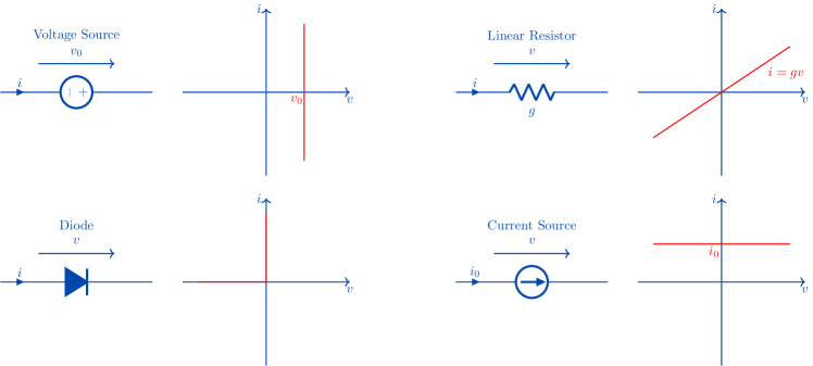
Figure 1: Ideal circuit elements and their current-voltage (i-v) characteristics. A linear resistor is characterized by Ohm’s law: $i=gv$, where $g$ is the conductance of the resistor ($g=1/r$ where $r$ is the resistance). An ideal diode is characterized by $i=0$ for $v\leq 0$ (”off-state”) and $v=0$ for $i>0$ (”on-state”). An ideal voltage source is characterized by $v=v_{0}$ for some constant voltage $v_{0}$ independent of the current $i$. An ideal current source is characterized by $i=i_{0}$ for some constant current $i_{0}$ independent of the voltage $v$.

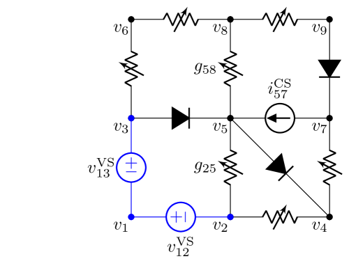
Figure 2: A nonlinear resistive network. By assumption, the voltage sources form a tree (in blue), so if we set e.g. $v_{1}=0$, we can immediately compute $v_{2}=-v_{12}^{\rm VS}$ and $v_{3}=v_{13}^{\rm VS}$. Next, we compute the steady state of the network by performing exact coordinate descent (Theorem 2) on the set of internal node electrical potentials (in black). As an example, one step of exact coordinate descent on node $k=5$ proceeds as follows. First we look at the resistors and current sources connected to node $k=5$ and we calculate $p_{5}=(g_{25}v_{2}+g_{58}v_{8}+i_{57}^{\rm CS})/(g_{25}+g_{58})$. Then we look at the diodes connected to node $k=5$ and we calculate $v_{5}=\max(v_{3},\min(p_{5},v_{4}))$. This is the value of $v_{5}$ that achieves the minimum of $E(v_{5})$ given other variables (node electrical potentials) fixed. We repeat the process with other nodes until convergence.

A nonlinear resistive network can be represented as a graph in which each branch contains a unique element - see Figure 2. We denote $\mathcal{B}=\mathcal{B}_{\rm VS}\cup\mathcal{B}_{\rm CS}\cup\mathcal{B}_{\rm R}\cup\mathcal{B}_{\rm D}$ the set of all branches, where $\mathcal{B}_{\rm VS}$ (resp. $\mathcal{B}_{\rm CS}$, $\mathcal{B}_{\rm R}$, $\mathcal{B}_{\rm D}$) is the subset of branches containing a voltage source (resp. current source, resistor, diode). For every $(j,k)\in\mathcal{B}_{\rm VS}$, we denote $v_{jk}^{\rm VS}$ the voltage across the voltage source between nodes $j$ and $k$. For every $(j,k)\in\mathcal{B}_{\rm CS}$, we denote $i_{jk}^{\rm CS}$ the current through the current source between nodes $j$ and $k$. Finally, for every $(j,k)\in\mathcal{B}_{\rm R}$, we denote $g_{jk}$ the conductance of the resistor between nodes $j$ and $k$.

We call ‘steady state’ a configuration of branch voltages and branch currents that verifies all of the above branch equations, as well as Kirchhoff’s current law (KCL) at every node, and Kirchhoff’s voltage law (KVL) in every loop. Under the above assumption of ideality, the steady state of a nonlinear resistive network is characterized by the following result – see Appendix A for a proof.

Theorem 1 (Convex QP formulation).

Consider a nonlinear resistive network with $N$ nodes, and denote $v=(v_{1},v_{2},\ldots,v_{N})$ the node electrical potentials. Under the above assumption of ideality, the steady state configuration of node electrical potentials, denoted $v_{\star}$, satisfies

$$v_{\star}=\underset{v\in\mathcal{S}}{\arg\min}\;E(v),$$ (1)

where $E:\mathbb{R}^{N}\to\mathbb{R}$ is the function defined by

$$E(v_{1},\ldots,v_{N}) :=\frac{1}{2}\sum_{(j,k)\in\mathcal{B}_{\rm R}}g_{jk}\left(v_{j}-v_{k}\right)^{2}$$ (2)

$$+\sum_{(j,k)\in\mathcal{B}_{\rm CS}}i_{jk}^{\rm CS}\left(v_{j}-v_{k}\right),$$ (3)

and $\mathcal{S}$ is the set:

$$\mathcal{S}:=\{ (v_{1},v_{2},\ldots,v_{N})\in\mathbb{R}^{N},$$ (4)

$$v_{j}\leq v_{k}\quad\forall(j,k)\in\mathcal{B}_{\rm D},$$ (5)

$$v_{j}=v_{k}+v_{jk}^{\rm VS}\quad\forall(j,k)\in\mathcal{B}_{\rm VS}\}.$$ (6)

A few comments are in order. First, we call $\mathcal{S}$ the set of feasible configurations of node electrical potentials (or the feasible set for short), and $E$ is the energy function of the network (or the objective function). Importantly, a configuration $v\in\mathcal{S}$ does not necessarily verify all the laws of electrical circuit theory - in other words, a feasible configuration is not necessarily the physically realized configuration. Similarly, the energy function $E$ is defined for every feasible configuration of node electrical potentials $v\in\mathcal{S}$, even those that do not comply with all the laws of electrical circuit theory. Theorem 1 states that among all feasible configurations, the one that is physically realized (the steady state) is the configuration that achieves the minimum of $E$.

Second, the feasible set $\mathcal{S}$ is defined by linear equality and inequality constraints. The constraint $v_{j}\geq v_{k}$ for every $(j,k)\in\mathcal{B}_{\rm D}$ states that the voltage $v_{j}-v_{k}$ across the diode is non-negative ($v_{j}>v_{k}$ if the diode is in off-state, and $v_{j}=v_{k}$ if the diode is in on-state), and the constraint $v_{j}=v_{k}+v_{jk}^{\rm VS}$ for every $(j,k)\in\mathcal{B}_{\rm VS}$ states that the voltage $v_{j}-v_{k}$ across the voltage source is $v_{jk}^{\rm VS}$. The diodes and voltage sources thus constrain the set of feasible configurations. We note that some conditions on the network topology and branch characteristics must be met to ensure that the feasible set $\mathcal{S}$ is non-empty: for instance, if the network contains a loop of voltage sources whose voltage drops do not add up to zero, then KVL is violated and the feasible set is empty.

Third, the energy function $E$ is half the total power dissipated in the resistors of the network, plus the total power dissipated in the current sources, with $g_{jk}\left(v_{j}-v_{k}\right)^{2}$ representing the power dissipated in the resistor of branch $(j,k)\in\mathcal{B}_{\rm R}$, and $i_{jk}^{\rm CS}\left(v_{j}-v_{k}\right)$ being the power dissipated in the current source of branch $(j,k)\in\mathcal{B}_{\rm CS}$. Our Theorem 1 generalizes Onsager’s well-known principle of minimum dissipated power which states that, in a linear resistor network (with voltage sources and linear resistors, but without diodes and current sources), among all feasible configurations of node electrical potentials, the one that is physically realized is the one that minimizes the power dissipated in the resistors (Onsager, 1931) – see also Baez & Fong (2018).

Finally, as a sum of convex functions, the energy $E(v)$ is a convex function of the node electrical potentials $v$. Specifically, the energy function $E(v)$ is a quadratic form in $v$, the Hessian of $E$ being positive definite. The feasible set $\mathcal{S}$, defined by linear constraints, is also convex. Therefore, Theorem 1 states that the steady state configuration of node electrical potentials is the solution of a convex optimization problem, specifically, a convex quadratic programming (QP) problem with linear constraints.

Next we turn to our algorithm for simulating (ideal) nonlinear resistive networks.

2.2 An algorithm to simulate nonlinear resistive networks

Equiped with the QP formulation (Theorem 1), we introduce a numerical method to compute the steady state $v_{\star}$ of an ideal nonlinear resistive network (1). Starting from some configuration $v^{(0)}\in\mathcal{S}$, our algorithm consists in minimizing the energy function $E(v)$ with respect to $v\in\mathcal{S}$ by building a sequence of configurations $v^{(1)},v^{(2)},\ldots,v^{(t)},\ldots$ in the feasible set $\mathcal{S}$ such that $E(v^{(t+1)})\leq E(v^{(t)})$ for every $t\geq 0$. Specifically, we use an ‘exact coordinate descent’ algorithm. The main ingredient of our algorithm is the result below.

For simplicity and clarity, we will assume here that the voltage sources form a connected component – a tree of the network – although our algorithm can be adapted to the more general case where the voltage sources form a forest (i.e a disjoint union of multiple trees).

Theorem 2 (Exact coordinate descent).

Let $v=(v_{1},\ldots,v_{N})\in\mathcal{S}$. Let $k$ be an internal node of the network, i.e. a node that does not belong to the connected component of voltage sources. Define

$$p_{k}:=\frac{\sum_{j\in\mathcal{B}_{\rm R}}g_{kj}v_{j}+\sum_{j\in\mathcal{B}_{\rm CS}}i_{jk}^{\rm CS}}{\sum_{j\in\mathcal{B}_{\rm R}}g_{kj}}$$ (7)

and

$$v_{k}^{\rm min}:=\max_{j:(j,k)\in\mathcal{B}_{\rm D}}v_{j},\qquad v_{k}^{\rm max}:=\min_{j:(k,j)\in\mathcal{B}_{\rm D}}v_{j},$$ (8)

$$v_{k}^{\prime}:=\min\left(\max\left(v_{k}^{\rm min},p_{k}\right),v_{k}^{\rm max}\right),$$ (9)

$$v^{\prime}:=(v_{1},\ldots,v_{k-1},v_{k}^{\prime},v_{k+1},\ldots,v_{N}).$$ (10)

Then, among all configurations $v^{\prime\prime}\in\mathcal{S}$ of the form $v^{\prime\prime}=(v_{1},\ldots,v_{k-1},v_{k}^{\prime\prime},v_{k+1},\ldots,v_{N})$, the configuration $v^{\prime}$ is the one with lowest energy, i.e.

$$v_{k}^{\prime}=\underset{v_{k}^{\prime\prime}\in\mathcal{S}}{\arg\min}\;E(v_{1},\ldots,v_{k-1},v_{k}^{\prime\prime},v_{k+1},\ldots,v_{N}).$$ (11)

In particular $v^{\prime}\in\mathcal{S}$ and $E(v^{\prime})\leq E(v)$.

We prove Theorem 2 in Appendix A. We provide an intuitive explanation of the result. Let $k$ such that $1\leq k\leq N$. The energy function $E$ of (2) is a quadratic function of $v_{k}$ given the state of other node electrical potentials fixed ($v_{1},\ldots,v_{k-1},v_{k+1},\ldots,v_{N}$). In other words, $E$ is of the form $E=a_{k}v_{k}^{2}+b_{k}v_{k}+c_{k}$ for some real-valued coefficients $a_{k}$, $b_{k}$ and $c_{k}$ that do not depend on $v_{k}$. Specifically, the values of $a_{k}$ and $b_{k}$ are $a_{k}:=\frac{1}{2}\sum_{j\in\mathcal{B}_{\rm R}}g_{jk}$ and $b_{k}:=-\sum_{j\in\mathcal{B}_{\rm R}}g_{kj}v_{j}-\sum_{j\in\mathcal{B}_{\rm CS}}i_{jk}^{\rm CS}$. Furthermore, the range of feasible values for $v_{k}$, constrained by the diodes, is of the form $[v_{k}^{\rm min},v_{k}^{\rm max}]$ where $v_{k}^{\rm min}$ and $v_{k}^{\rm max}$ are given by (8). Since the coefficient $a_{k}$ is positive (as a sum of conductances), the energy $E(v_{k})$ is bounded below and its minimum in $\mathbb{R}$ is obtained at the point $p_{k}:=-b_{k}/2a_{k}$. Similarly, it is easily seen that the minimum of $E(v_{k})$ in the interval $[v_{k}^{\rm min},v_{k}^{\rm max}]$ is obtained by clipping $p_{k}$ between $v_{k}^{\rm min}$ and $v_{k}^{\rm max}$. These boundaries reflect the constraints imposed by the diodes connected to node $k$, introducing nonlinearities.

Using Theorem 2, we can then minimize the energy function $E$ via an ‘exact coordinate descent’ strategy. Assuming that the feasible set $\mathcal{S}$ is not empty, we start from some feasible configuration $v\in\mathcal{S}$. Then, at each step, we pick some internal node $k$, and we compute the value $v_{k}^{\prime}$ that minimizes $E$ given the values of other variables fixed, using Theorem 2. We obtain a new feasible configuration $v^{\prime}\in\mathcal{S}$. Then we pick another variable and we repeat the process. At each step of the process, the energy $E$ cannot increase.

3 Deep resistive networks

We now turn to the deep resistive network (DRN) model, a layered nonlinear resistive network architecture introduced in Kendall et al. (2020). We consider here more specifically the DRN variant of Scellier & Mishra (2023). DRNs, which take inspiration from the architecture of layered neural networks, present advantages for hardware design as they are potentially amenable for implementation using crossbar arrays of memristors (Xia & Yang, 2019). In this section, we show that ideal DRNs also present advantages in terms of simulation speed, when our algorithm is executed on multi-processor computers such as GPUs.

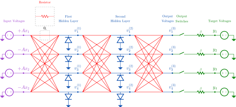
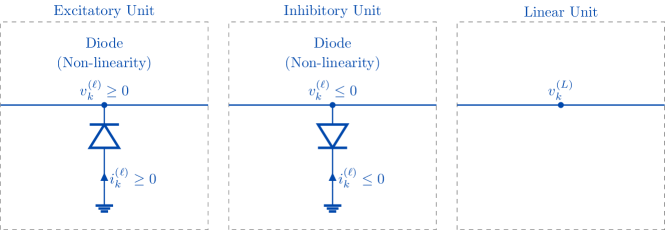
Figure 3: Top. A deep resistive network (DRN) with $L=3$ layers. Input voltage sources are set to input values: $v_{1}^{(0)}=Ax_{1}$, $v_{2}^{(0)}=-Ax_{1}$, $v_{3}^{(0)}=Ax_{2}$ and $v_{4}^{(0)}=-Ax_{2}$, where $A$ is the input amplification factor. At inference, output switches are open. Equilibrium propagation learning requires nudging the output node voltages ($v_{1}^{(3)}$, $v_{2}^{(3)}$ $v_{3}^{(3)}$ and $v_{4}^{(3)}$) towards the target voltages ($y_{1}$, $y_{2}$, $y_{3}$ and $y_{4}$), which is achieved by closing the output switches. In the DRN architecture, the update rule for a given unit prescribed by exact coordinate descent depends only on the states of the units of the previous layer and the next layer. We can thus update the even layers ($\ell=2$) simulatneously, and then update all the odd layers ($\ell=1$ and $\ell=3$) simultaneously. This is called exact block coordinate descent. Bottom. To form a nonlinear unit, we place a diode between the unit’s node and ground. Depending on the orientation of the diode, the units come in two flavours: excitatory units and inhibitory units.

3.1 Deep resistive network architecture

The DRN architecture is defined as follows. First of all, we choose a reference node called ‘ground’. A set of nodes connected to ground by voltage sources form the ‘input layer’. These voltage sources can be set to input values, playing the role of input variables. Another set of nodes form the ‘output layer’ whose electrical potentials play the role of model outputs.

Energy function.

In a DRN, the circuit elements (voltage sources, resistors, diodes and current sources) are assembled into a layered network, mimicking the architecture of a deep neural network (Figure 3). For each $\ell$ such that $0\leq\ell\leq L$, we denote $N_{\ell}$ the number of nodes in layer $\ell$, where $L$ is the number of layers in the DRN. Each node in the network is also called a ‘unit’ by analogy with a neural network. We denote $v_{k}^{(\ell)}$ the electrical potential of the $k$-th node of layer $\ell$, which we may think of as the unit’s activation. Pairs of nodes from two consecutive layers are interconnected by variable resistors - the ‘trainable weights’. Denoting $g_{jk}^{(\ell)}$ the conductance of the variable resistor between the $j$-th node of layer $\ell-1$ and the $k$-th node of layer $\ell$, the energy function (2) of a DRN takes the form

$$E(v)=\frac{1}{2}\sum_{\ell=1}^{L}\sum_{j=1}^{N_{\ell-1}}\sum_{k=1}^{N_{\ell}}g_{jk}^{(\ell)}\left(v_{j}^{(\ell-1)}-v_{k}^{(\ell)}\right)^{2}.$$ (12)

Feasible set.

The voltage sources and resistors being linear elements, the network built thus far is linear. To make it nonlinear, we use diodes. For each unit, we place a diode between the unit’s node and ground, which can be oriented in either of the two directions. If the diode points from ground to the unit’s node, the unit’s electrical potential is non-negative: we call it an ‘excitatory unit’. Conversely, if the diode points from the unit’s node to ground, the unit’s electrical potential is non-positive: we call it an ‘inhibitory unit’. For each internal (‘hidden’) layer $\ell$ of the DRN ($1\leq\ell\leq L-1$), we orient the diodes so that the units of even indices are excitatory and the units of odd indices are inhibitory. Finally, the units of the output layer ($\ell=L$) are linear, i.e. they do not possess diodes. The feasible set (4) corresponding to this DRN architecture is

$$\mathcal{S}=\{v\in\mathbb{R}^{\sum_{\ell=1}^{L}N_{\ell}}\mid v_{k}^{(\ell)}\geq 0\text{ if k is even},$$ (13)

$$v_{k}^{(\ell)}\leq 0\text{ if k is odd},1\leq\ell\leq L-1,1\leq k\leq N_{\ell}\}.$$ (14)

Input voltage sources.

One constraint with resistive networks in general, and deep resistive networks in particular, is the non-negativity of the weights - a conductance is non-negative. By using both excitatory units and inhibitory units in the hidden layers, we have partially overcome this constraint. To further enhance the representational capacity of the DRN, we also double the number of units in the input layer – i.e. we choose $N_{0}=2\dim(x)$ where $\dim(x)$ is the dimension of input $x$ – and we set the input voltage sources such that $v_{2k}^{(0)}=-v_{2k-1}^{(0)}$ for each $1\leq k\leq N_{0}$. Another constraint with DRNs is the decay in amplitude of the layers’ voltage values, as the depth of the network increases. We overcome this constraint by amplifying the input voltages by a factor $A\gg 1$, so that $v_{2k-1}^{0}=+Ax_{k}$ and $v_{2k}^{0}=-Ax_{k}$ for every $k$, where $x_{k}$ is the $k$-th input value ($1\leq k\leq N_{0}$).

Output switches.

Finally, additional circuitry is needed for equilibrium propagation (EP) learning. Each output node is linked to ground via a switch in series with a resistor and a voltage source. The voltage sources are used to set the desired output values, playing the role of targets. The resistors all share a common conductance value $\beta>0$. During inference, the switches are open, whereas in the training phase of EP, the switches are closed to drive the state of output units towards the desired output values – see Appendix B for a brief presentation of EP (Scellier & Bengio, 2017).

3.2 A fast algorithm to simulate deep resistive networks

In a DRN, the update rules (Theorem 2) for the units take the following form. For every $(\ell,k)$ such that $1\leq\ell\leq L-1$ and $1\leq k\leq N_{\ell}$, the update rule for $v_{k}^{(\ell)}$ is

$$p_{k}^{(\ell)}:=\frac{\sum_{j=1}^{N_{\ell-1}}g_{jk}^{(\ell)}v_{j}^{(\ell-1)}+\sum_{j=1}^{N_{\ell+1}}g_{kj}^{(\ell+1)}v_{j}^{(\ell+1)}}{\sum_{j=1}^{N_{\ell-1}}g_{jk}^{(\ell)}+\sum_{j=1}^{N_{\ell+1}}g_{kj}^{(\ell+1)}}$$ (15)

$$v_{k}^{(\ell)}\leftarrow\left\{\begin{array}[]{l}\displaystyle\max\left(0,p_{k}^{(\ell)}\right)\qquad\text{if k is even (excitatory unit)},\\ \displaystyle\min\left(0,p_{k}^{(\ell)}\right)\qquad\text{if k is odd (inhibitory unit)}.\end{array}\right.$$ (18)

Assuming that the output switches are closed, the update rule for the output unit $v_{k}^{(L)}$ is

$$v_{k}^{(L)}\leftarrow\frac{\sum_{j=1}^{N_{\ell-1}}g_{jk}^{(L)}v_{j}^{(L-1)}+\beta y_{k}}{\sum_{j=1}^{N_{\ell-1}}g_{jk}^{(L)}+\beta}.$$ (19)

If the output switches are open, Equation (19) still holds by setting $\beta=0$.

We now derive a specialized, fast algorithm to compute the steady state of a DRN. Since the update rule for $v_{k}^{(\ell)}$ depends only on the state of the units in layers $\ell-1$ and $\ell+1$, and since this is true for all the units in layer $\ell$, we may update all these units simultaneously rather than sequentially. Pushing this idea further, we can partition the layers of the network in two groups: the group of layers of even index (even $\ell$) and the group of layers of odd index (odd $\ell$). Since the update rules for the odd layers depend only on the state of even layers, and vice versa, we can compute the steady state of a DRN by updating alternatively the layers of odd indices (given the state of the layers of even indices fixed) and the layers of even indices (given the state of the layers of odd indices fixed). We obtain an ‘exact block coordinate descent’ algorithm to simulate DRNs. The property of DRNs that make it possible is the bipartite structure of their graph, where the layers of even indices constitute one set, and the layers of odd indices constitute the other set.

Importantly, equations (15) and  (19) can be written in matrix-vector form. Each step of our exact block coordinate descent algorithm (updating half of the layers) thus consists in performing $\sim L$ matrix-vector multiplications, $\sim L/2$ divisions and $\sim L/2$ clipping operations. This makes it an algorithm ideally suited to run on parallel computing platforms such as GPUs.

We note that it is possible to further speed up the simulations of DRNs by computing the row-wise sums of the weight matrices (used at the denominator of the update rules) only once for each inference (steady state computation), instead of computing it at each iteration of the algorithm.

4 Simulations

We use our exact block coordinate descent algorithm to train deep resistive networks (DRNs) with equilibrium propagation (EP) (Scellier & Bengio, 2017) on the MNIST classification task. We train DRNs of one, two and three hidden layers, denoted DRN-1H, DRN-2H and DRN-3H, respectively. We also train a DRN with a single hidden layer of 32784 units, denoted DRN-XL, which is 325x larger than the model in Kendall et al. (2020). EP is presented in Appendix B and a full description of the DRN models and the hyperparameters used for training are provided in Appendix C. We also benchmark EP-trained DRNs against backpropagation-trained (BP-trained) DRNs. We used a single A100 GPU to run these simulations.

Table 1: We trained four deep resistive network (DRN) architectures (XL, 1H, 2H and 3H) on MNIST. The size of the network, as measured per the number of weights (in millions), is written in brackets. Alg refers to the training algorithm: equilibrium propagation (EP) or backpropagation (BP). Our exact block coordinate descent method was used to compute the DRN steady states required for EP and BP training. Test refers to the test error rates (in %). For each experiment, we performed five runs and we reported the mean values and std values. We also reported the number of epochs of training and the wall-clock time (WCT). A full description of the models with the hyperparameters used for training are reported in Table 2 of Appendix C. We also report the results of the SPICE-based simulations of Kendall et al. (2020) as a baseline, denoted XS.

DRN	Alg	Test (%)	Epochs	WCT
XS (0.16M)	EP	3.43	10	1 week
XL (51.7M)	EP	1.40 $\pm$ 0.03	50	5:20
	BP	1.40 $\pm$ 0.02	50	3:58
1h (1.6M)	EP	1.57 $\pm$ 0.07	50	2:50
	BP	1.54 $\pm$ 0.04	50	2:48
2h (2.7M)	EP	1.48 $\pm$ 0.05	50	5:15
	BP	1.45 $\pm$ 0.08	50	5:07
3h (3.7M)	EP	1.66 $\pm$ 0.09	50	7:41
	BP	1.50 $\pm$ 0.07	50	8:01

Table 1 shows the results. The largest network that we train (the DRN-XL model) has 325 times as many parameters as the DRN architecture used in Kendall et al. (2020) (51.7M vs 0.16M). We train it for 5 times as many epochs (50 vs 10) and the total duration of training is 30 times shorter (5 hours 20 min vs 1 week). Thus, our network-size-to-epoch-duration ratio is 50000x larger. The performance obtained with the DRN-XL model is also significantly better (1.40% vs 3.43% test error rate).

5 Discussion

As nonlinear resistive networks have recently attracted interest as physical (analog) self-learning machines, efficiently simulating these networks has become critical to advance research in this direction. Previous works either used general purpose circuit simulators such as SPICE – which are are extremely slow as they were not specifically conceived for the simulations of nonlinear resistive networks – or resorted to linear networks, which are easier to simulate but lack a crucial feature of machine learning: nonlinearity. In this work, we have introduced a methodology specifically tailored for the simulations of nonlinear resistive networks. We have shown that the problem of determining the steady state of a nonlinear resistive network can be formulated as a convex quadratic programming (QP) problem, where the objective function is the power dissipated in the resistors, and the feasible set of node electrical potentials reflects the inequality constraints imposed by the diodes. Using this formulation, we have introduced an efficient algorithm to simulate nonlinear resistive networks with arbitrary network topologies, based on ‘exact coordinate descent’ (Wright, 2015). In the case of layered networks - deep resistive networks (DRNs) - we took advantage of the bipartite structure of the network to derive an exact block coordinate descent algorithm where half of the coordinates (node electrical potentials) are updated at each step. Each step of our algorithm involves solely matrix-vector multiplications, divisions and clipping, making it ideal to run on parallel processors such as GPUs. Compared to the SPICE-based simulations of Kendall et al. (2020), the largest networks that we trained are 325 times larger, and simulating them (on a single A100 GPU) was 150 times faster. Training larger networks for more epochs also helped us achieve significantly better results on the MNIST dataset (1.40% vs 3.43% test error).

Although we have primarily focused on layered architectures (DRNs), our algorithm applies to arbitrary network topologies, including unstructured (disordered) networks (Stern et al., 2022, 2023; Wycoff et al., 2022). In such networks, parallelization is also possible, although it is less straightforward to implement. More generally, our characterization of the steady state as the solution of a quadratic programming (QP) problem with linear constraints offers other options to simulate nonlinear resistive networks. Indeed, QP problems can be solved with various algorithms, such as primal-dual interior point methods (IPM) and sequential quadratic programming (SQP) methods. Many optimization libraries and software packages provide specialized QP solvers. Besides, while in our simulations we have used equilibrium propagation (EP) for training, our exact coordinate descent algorithm for nonlinear resistive networks can be used in conjunction with other learning algorithms such as frequency propagation (Anisetti et al., 2022) and agnostic EP (Scellier et al., 2022). It can also be used in conjunction with e.g. the method proposed by Stern et al. (2023) to mitigate power dissipation.

While our methodology to simulate nonlinear resistive networks is fairly general, it is also important to acknowledge the limitations of our approach. Our methodology is anchored in an assumption of ideality of the circuit elements (resistors, diodes, voltage sources and current sources). Real-world diodes, however, deviate significantly from the ideal model studied here: they have a forward voltage drop, reverse leakage current, non-zero resistance when forward-biased, and a breakdown voltage when reverse-biased. Despite these assumptions, which may seem overly simplistic, we believe that our algorithm can be usefully applied to prototype and explore a wide range of network topologies.

We note that nonlinear resistive networks and DRNs are also closely related to continuous Hopfield networks (Hopfield, 1984) and deep (layered) Hopfield networks (DHNs) (Scellier & Bengio, 2017), respectively. In particular, our exact coordinate descent algorithm for resistive networks is similar in spirit to the asynchronous update scheme for Hopfield networks, and our exact block coordinate descent algorithm for DRNs is also similar to the asynchronous energy minimization scheme for DHNs (Scellier et al., 2023) and to block-Gibbs sampling in deep Boltzmann machines (Salakhutdinov & Hinton, 2009). Importantly, unlike Hopfield networks and Boltzmann machines whose energy functions are typically non-convex, the energy function (power dissipation) of a nonlinear resistive network is convex. In practice we find that our DRN simulations require much fewer steps to converge than in DHNs. The connection between resistive networks and Hopfield networks is especially interesting as recent works have shown that DHNs yield promising results on image classification tasks such as CIFAR-10 (Laborieux et al., 2021), CIFAR-100 (Scellier et al., 2023) and ImageNet 32x32 (Laborieux & Zenke, 2022).

Looking forward, we contend that our simulation methodology can foster more rapid progress in nonlinear resistive network research. It offers the perspective to perform large scale simulations of (ideal) deep resistive networks (DRNs), to enable further assessment of the scalability of such physical (analog) self-learning machines, and perhaps guide their hardware design too.

Appendix A Proofs

In this appendix, we prove Theorem 1 and Theorem 2.

First we recall our assumptions about the behaviour of individual devices. We consider four types of elements - linear resistors, diodes, voltage sources and current sources - with the following current-voltage (i-v) characteristics:

• A linear resistor follows Ohm’s law, i.e. $i=gv$ where $g$ is the conductance of the resistor ($g=1/r$ where $r$ is the resistance).

• A diode satisfies $i=0$ for $v\leq 0$, and $v=0$ for $i>0$.

• A voltage source satisfies $v=v_{0}$ for some constant $v_{0}$, regardless of $i$.

• A current source satisfies $i=i_{0}$ for some constant $i_{0}$, regardless of $v$.

A.1 Proof of Theorem 1

We denote $v^{\rm VS}$ the set of voltages across voltage sources, and $i^{\rm CS}$ the set of currents across current sources. For clarity and ease of reading, we repeat Theorem 1.

See 1

Proof of Theorem 1.

Suppose that there exists a configuration of branch voltages and branch currents that satisfies all the current-voltage constraints in every branch, as well as Kirchhoff’s current law (KCL) and Kirchhoff’s voltage law (KVL). We call this configuration ‘steady state’ and we denote $v_{\star}=(v_{1},\ldots,v_{N})$ the corresponding configuration of node electrical potentials, where $N$ is the number of nodes in the network. For every branch $(j,k)\in\mathcal{B}_{\rm R}$ (resp. $\mathcal{B}_{\rm D}$, $\mathcal{B}_{\rm VS}$), we denote $i_{jk}^{\rm R}$ (resp. $i_{jk}^{\rm D}$, $i_{jk}^{\rm VS}$) the current through it. The resistor’s equation (Ohm’s law) imposes that

$$\forall(j,k)\in\mathcal{B}_{\rm R},\qquad i_{jk}^{\rm R}=g_{jk}(v_{j}-v_{k}).$$ (20)

Let us define the functions $G_{jk}$ (for $(j,k)\in\mathcal{B}_{\rm D}$) and $H_{jk}$ (for $(j,k)\in\mathcal{B}_{\rm VS}$) as

$$\forall(j,k)\in\mathcal{B}_{\rm D},\quad G_{jk}(v):=v_{j}-v_{k}\qquad\text{and}\qquad\forall(j,k)\in\mathcal{B}_{\rm VS},\quad H_{jk}(v):=v_{j}-v_{k}-v_{jk}^{\rm VS}.$$ (21)

The diode equations impose that

$$\forall(j,k)\in\mathcal{B}_{\rm D},\qquad G_{jk}(v)\leq 0,\qquad i_{jk}^{\rm D}\geq 0,\qquad i_{jk}^{\rm D}\cdot G_{jk}(v)=0.$$ (22)

The voltage source equality constraints impose that

$$\forall(j,k)\in\mathcal{B}_{\rm VS},\qquad H_{jk}(v)=0.$$ (23)

Next, let $k$ such that $1\leq k\leq N$, and consider all the branches connected to node $k$. There are four kinds of such branches: resistors, current sources, diodes and voltage sources. KCL applied to node $k$ reads

$$\sum_{j:(j,k)\in\mathcal{B}_{\rm R}}i_{jk}^{\rm R}+\sum_{j:(j,k)\in\mathcal{B}_{\rm CS}}i_{jk}^{\rm CS}+\sum_{j:(j,k)\in\mathcal{B}_{\rm D}}i_{jk}^{\rm D}+\sum_{j:(j,k)\in\mathcal{B}_{\rm VS}}i_{jk}^{\rm VS}=0.$$ (24)

Let us introduce the following function $L$, which is a function of the node electrical potentials ($v$), the currents through the diodes ($i^{\rm D}$), and the currents through the voltage sources ($i^{\rm VS}$),

$$L(v,i^{\rm D},i^{\rm VS}):=E(v)+\sum_{(j,k)\in\mathcal{B}_{\rm D}}i_{jk}^{\rm D}G_{jk}(v)+\sum_{(j,k)\in\mathcal{B}_{\rm VS}}i_{jk}^{\rm VS}H_{jk}(v).$$ (25)

Using the expressions of the energy function (2) and the functions $G_{jk}$ and $H_{jk}$ of (21), KCL (24) rewrites in terms of $L$ as

$$\nabla_{v}L(v,i_{jk}^{\rm D},i_{jk}^{\rm VS})=0.$$ (26)

Equations (22), (23) and (26) fully characterize the steady state of the nonlinear resistive network. These equations constitute the set of Karush-Kuhn-Tucker (KKT) conditions associated to the constrained optimization problem (1). $L$ is the Lagrangian, and the currents $i^{\rm D}$ and $i^{\rm VS}$ are the Lagrange multipliers associated to the inequality and equality constraints, respectively. Equations (22) and (23) constitute the primal feasibility condition ($v$ must belong to the feasible state $\mathcal{S}$), dual feasibility condition (the Lagrange multipliers associated with the inequality constraints must be non-negative), and the complementary slackness for inequality constraints (either the constraint is ‘binding’ or the associated Lagrange multiplier is zero). Finally, (26) is the stationarity condition of the Lagrangian.

From the above analysis, it follows that the steady state of the network (if it exists) satisfies the KKT conditions associated to the constrained optimization problem (1). Conversely, a configuration of node voltages and branch currents (diode branches and voltage source branches) that satisfies the KKT conditions is a steady state.

To conclude, we note that, as a sum of convex (quadratic) functions, the energy function $E$ is convex (quadratic). Therefore the KKT conditions are equivalent to global optimality. This implies that a steady state exists if and only if the feasible set is non-empty, in which case the corresponding configuration of node voltages is a global minimum of the convex optimization problem. ∎

A.2 Proof of Theorem 2

The optimization problem is a quadratic programming (QP) problem with linear constraints. We solve it using exact coordinate descent.

See 2

Proof of Theorem 2.

The energy as a function of $v_{k}$ is of the form

$$E(v_{k}) =\frac{1}{2}\sum_{j:(j,k)\in\mathcal{B}_{\rm R}}g_{jk}\left(v_{j}-v_{k}\right)^{2}+\sum_{j:(j,k)\in\mathcal{B}_{\rm CS}}i_{jk}^{\rm CS}(v_{j}-v_{k})$$ (27)

$$=\underbrace{\left(\frac{1}{2}\sum_{j:(j,k)\in\mathcal{B}_{\rm R}}g_{jk}\right)}_{=:a_{k}}v_{k}^{2}-\underbrace{\left(\sum_{j:(j,k)\in\mathcal{B}_{\rm R}}g_{kj}v_{j}+\sum_{j:(j,k)\in\mathcal{B}_{\rm CS}}i_{jk}^{\rm CS}\right)}_{=:b_{k}}v_{k}+\text{constant}$$ (28)

The minimum of $E(v_{k})$ with respect to $v_{k}$ in $\mathbb{R}$ is achieved at the point

$$p_{k}:=-\frac{b_{k}}{2a_{k}}=\frac{\sum_{j:(j,k)\in\mathcal{B}_{\rm R}}g_{kj}v_{j}+\sum_{j:(j,k)\in\mathcal{B}_{\rm CS}}i_{jk}^{\rm CS}}{\sum_{j:(j,k)\in\mathcal{B}_{\rm R}}g_{jk}}.$$ (29)

Besides, the range of feasible values for $v_{k}$ (in the feasible set $\mathcal{S}$) is $(v_{k}^{\rm min},v_{k}^{\rm max})$, where

$$v_{k}^{\rm min}:=\max_{j:(j,k)\in\mathcal{B}_{\rm D}}v_{j},\qquad v_{k}^{\rm max}:=\min_{j:(k,j)\in\mathcal{B}_{\rm D}}v_{j}.$$ (30)

The value $v_{k}^{\prime}\in(v_{k}^{\rm min},v_{k}^{\rm max})$ that minimizes the energy function $E$ (given other variables fixed) is

$$v_{k}^{\prime}:=\min\left(\max\left(v_{k}^{\rm min},p_{k}\right),v_{k}^{\rm max}\right).$$ (31)

∎

Appendix B Equilibrium propagation

In this appendix, we briefly present the equilibrium propagation (EP) algorithm (Scellier & Bengio, 2017). While in this work we have used EP to train DRNs (section 4), EP is applicable to any nonlinear resistive network.

In general, a nonlinear resistive network can be utilized for computation, whereby

• a set of voltage sources serve as ‘input variables’ whose voltages play the role of input values,

• a set of branches function as ‘output variables’ whose voltages are used as the model’s prediction.

Computing with such a nonlinear resistive network proceeds as follows: 1) set the input voltage sources to input values, 2) let the electrical network reach steady state, i.e. a minimum of the energy function (2), and 3) read the output voltages across the output branches. The input-output function computed by this electrical network can be seen as parameterized by the conductances of the (variable) resistors. The problem of training the network then consists in modifying the conductance values of the variable resistors (the ‘weights’) so that the network computes a desired input-output function. Several learning algorithms for resistive networks have been proposed (Kendall et al., 2020; Dillavou et al., 2022; Anisetti et al., 2022) based on EP. Here, we present EP.

First and foremost, EP learning necessitates augmenting the network. For each pair of output nodes, a new branch is introduced between the two nodes (in parallel to any existing branch), containing a voltage source, a resistor, and a switch in series (see Figure  4). All resistors have a common conductance value, $\beta>0$. Switches can either be open (we call it the ‘free state’) or closed (the ‘perturbed state’). When the output switches are open, the new output branches do not influence the network’s state. However, closing the output switches perturbs the network’s state: mathematically, the network’s energy function ($E$) gets augmented by a term equivalent to the power dissipated in the output resistors, $\frac{1}{2}\sum_{(j,k)\in\mathcal{B}_{\rm O}}\beta\left(v_{jk}-y_{jk}\right)^{2}$, with $\mathcal{B}_{O}$ denoting the set of output branches, and $y_{jk}$ signifying the voltage drop across the voltage source of output branch $(j,k)$.

For an input-output pair from training data, EP operates in three steps. In the first step, input voltage sources are set to the input values ($x$) and the output switches are open, so the network reaches the ‘free’ state

$$v_{\star}^{0}:=\underset{v\in\mathcal{S}}{\arg\min}\;E(v).$$ (32)

In the second step, output voltage sources are set to the desired output values ($y$) and the output switches are closed, so the network reaches a new ‘perturbed’ state

$$v_{\star}^{\beta}:=\underset{v\in\mathcal{S}}{\arg\min}\;\left[E(v)+\beta C(v)\right],$$ (33)

where

$$C(v):=\frac{1}{2}\sum_{(j,k)\in\mathcal{B}_{\rm O}}\left(v_{jk}-y_{jk}\right)^{2}.$$ (34)

The quantity $E+\beta C$ in (34) represents the effective energy function (power dissipation) of the augmented circuit. Importantly, the function $C$ appearing in this augmented energy is the squared error between the model prediction and the desired output, which can be seen as the cost function that the network must minimize from a learning perspective. Finally, in the third step, for every branch $(j,k)$ containing a resistor, the EP learning rule for the conductance $g_{jk}$ reads

$$\Delta g_{jk}:=\frac{\eta}{2\beta}\left[\left(v_{jk}^{0}\right)^{2}-\left(v_{jk}^{\beta}\right)^{2}\right],$$ (35)

where $\eta>0$ is the learning rate. The main result of the EP algorithm is that the learning rule (35) approximates one step of gradient descent on the cost function $C$ (Scellier & Bengio, 2017). More specifically, the EP learning rule (35) performs one step of gradient descent on a surrogate function $\mathcal{L}_{\beta}$ that approximates the true cost function $C$ (Scellier et al., 2023), i.e.

$$\Delta g_{jk}=-\eta\frac{\partial\mathcal{L}_{\beta}}{\partial g_{jk}}\qquad\text{where}\qquad\mathcal{L}_{\beta}=C(v_{\star}^{0})+O(\beta)\text{ when }\beta\to 0.$$ (36)

The surrogate function can be expressed as

$$\mathcal{L}_{\beta}:=\frac{F(\beta)-F(0)}{\beta},\qquad\text{where}\qquad F(\beta):=\min_{v}\left[E(v)+\beta C(v)\right].$$ (37)

The version of the EP algorithm described above, which uses the two states $v_{\star}^{0}$ and $v_{\star}^{\beta}$ ($\beta>0$), does not work very well in practice because the surrogate function $\mathcal{L}_{\beta}$ of the learning rule (35) is a lower bound of the true cost function $C$ (Scellier et al., 2023). The centered variant of EP (Laborieux et al., 2021), which combines a negatively-perturbed state $v_{\star}^{-\beta}$ with a positively-perturbed one $v_{\star}^{+\beta}$, proves much more effective in practice, performing gradient descent on a surrogate function $\mathcal{L}_{-\beta;\beta}$ that approximates the cost function at the second order in $\beta$, i.e. $\mathcal{L}_{-\beta;\beta}=C(v_{\star}^{0})+O(\beta^{2})$.

The method described above to augment the circuit – which uses a switch, a resistor and a voltage source in series in every output branch – does not allow for negative perturbations ($\beta<0$) since a conductance is always non-negative. To achieve negative perturbations, we need a different layout. We may use current sources whose current values are set to $i_{jk}=-\beta(v_{jk}-y_{jk})$, where $\beta\in\mathbb{R}$ (Figure  4). During inference (at test time), current sources are set to zero, behaving like open switches.

Remark. In the DRN architecture, input voltage sources link input nodes to ground, and output branches link output nodes to ground.

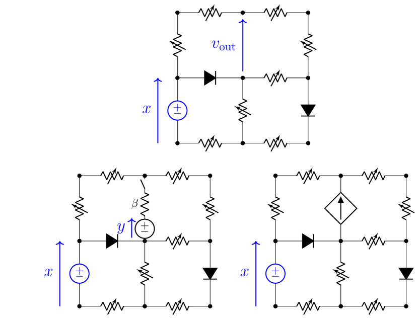
Figure 4: Training a nonlinear resistive network with equilibrium propagation (EP). Top. Given an input voltage $x$, the network computes the output voltage $v_{\rm out}$. Bottom. Two methods to implement ‘nudging’ for EP learning. In the first implementation (left), the output branch contains a voltage source set to the desired output $y$, in series with a resistor of conductance $\beta$ and a switch. Closing the switch results in injecting a current $\beta(y-v_{\rm out})$ in the branch, proportional to the prediction error. The drawback of this method is that the nudging factor $\beta$ is necessarily positive (a conductance is positive). In the second implementation (right), the output branch contains a current source set to $\beta(y-v_{\rm out})$. This implementation allows us to choose a negative nudging factor $\beta$.

Appendix C Simulation details

We provide the implementation details to reproduce the results of our simulations of DRNs trained by equilibrium propagation (EP) and backpropagation (BP). The code to reproduce the results is available at https://github.com/rain-neuromorphics/energy-based-learning

MNIST dataset.

The MNIST dataset of handwritten digits (LeCun et al., 1998) is composed of 60,000 training examples and 10,000 test examples. Each example $x$ in the dataset is a $28\times 28$ gray-scaled image and comes with a label $y\in\left\{0,1,\ldots,9\right\}$ indicating the digit that the image represents.

Network architectures.

We train four deep resistive network (DRN) models termed DRN-1H, DRN-2H, DRN-3H and DRN-XL. Each DRN has 1568 input units ($2\times 28\times 28$) and 10 output units corresponding to the ten classes of the MNIST dataset. The DRN-kH model has k hidden layers of 1024 units each ($k\in\{1,2,3\}$). The DRN-XL model has one hidden layer of 32768 units. Table 2 contains the architectural details of the four DRN models, as well as the hyperparameters used to obtain the results presented in Table 1.

Initialization of the conductances (‘weights’).

Given two consecutive layers of size $N_{\ell}$ and $N_{\ell+1}$, we initialize the matrix of conductances between these two layers according to a modified ‘Kaiming uniform’ initialization scheme:

$$g_{ij}^{(\ell+1)}\sim\max(0,w),\qquad w\sim\mathcal{U}(-c,+c),\qquad c=\sqrt{\frac{1}{N_{\ell}}}.$$ (38)

Input amplification factor.

We recall that, in a DRN, not only the number of input nodes (input voltage sources) is doubled, but input signals are amplified by a fixed gain factor $A>0$. For each DRN model (DRN-1H, DRN-2H, DRN-3H and DRN-XL), the choice of $A$ is reported in Table 2. We notice that the values of $A$ are relatively large, e.g. $A=4000$ for the DRN-3H model. We note that, instead of amplifying input signals of a DRN by a large amplification factor $A\gg 1$, another option is to use so-called bidirectional amplifiers at every layer (Kendall et al., 2020) – see appendix D for explanations.

Energy minimization.

To compute the steady state of the network, we use our exact block coordinate descent algorithm for DRNs (Section 3.2). At every iteration, we update the layers one by one from the input layer to the output layer. Relaxing every layer once (from input to output) constitutes one ‘iteration’. We repeat as many iterations as is necessary until convergence to the steady state. In Table 2, we denote $T$ the number of iterations performed at inference (free phase), and we denote $K$ the number of iterations performed in the second (training) phase.

Training procedure.

We train our networks with equilibrium propagation (EP, Appendix B) and backpropagation (BP). At each training step, we proceed as follows. First we pick a mini-batch of samples in the training set, $x$, and their corresponding labels, $y$. Then we perform $T$ iterations of the block coordinate descent algorithm without nudging ($\beta=0$). This phase allows us in particular to compute the training loss and training error rate for the current mini-batch, to monitor training. We also store the steady state (free state) $v_{\star}$. Next, we set the nudging parameter to $\beta$ and we perform a new block-coordinate descent of $K$ iterations, to compute the positively-perturbed state $v_{\star}^{\beta}$. Then, we reset the state of the network to the free state $v_{\star}$, we set the nudging parameter to the $-\beta$, and we perform the a new block-coordinate descent of $K$ iterations to compute the negatively-perturbed state $v_{\star}^{-\beta}$. Finally, we update all the conductances simultaneously, in proportion to the EP learning rule.

Optimizer and scheduler.

We use standard mini-batch gradient descent (SGD) with batch size 4. No momentum or weight decay is used. We use a scheduler with a decay of $0.99$ for the learning rates at each epoch of training.

Computational resources.

The code for the simulations uses PyTorch 1.13.1 and TorchVision 0.14.1. (Paszke et al., 2017). The simulations were carried on a single Nvidia A100 GPU.

Table 2: Hyper-parameters used for initializing and training the four DRN models (DRN-XL, DRN-1H, DRN-2H and DRN-3H) and reproducing the results of Table 1. LR means ‘learning rate’.

	DRN-XL	DRN-1H	DRN-2H	DRN-3H
Input amplification factor ($A$)	800	480	2000	4000
Nudging ($\beta$)	1.0	1.0	1.0	2.0
Num. iterations at inference ($T$)	4	4	5	6
Num. iterations during training ($K$)	4	4	5	6
Layer 0 (input) size ($N_{0}$)	2-28-28	2-28-28	2-28-28	2-28-28
Layer 1 size ($N_{1}$)	32768	1024	1024	1024
Layer 2 size ($N_{2}$)	10	10	1024	1024
Layer 3 size ($N_{3}$)			10	1024
Layer 4 size ($N_{4}$)				10
lr weight 1 & bias 1 ($\eta_{1}$)	0.006	0.006	0.002	0.005
lr weight 2 & bias 2 ($\eta_{2}$)	0.006	0.006	0.006	0.02
lr weight 3 & bias 3 ($\eta_{3}$)			0.018	0.08
lr weight 4 & bias 4 ($\eta_{4}$)				0.005
lr decay	0.99	0.99	0.99	0.99
Mini-batch size	4	4	4	4
Number of epochs	50	50	50	50

Appendix D Bidirectional amplifiers

One constraint of deep resistive networks (DRNs) is the decay in amplitude across the layers of the network, as the depth increases, and therefore the need to amplify the input voltages by a large gain $A\gg 1$ to compensate for this decay. Instead of amplifying input voltages by a large factor $A$, another avenue proposed in Kendall et al. (2020) is to equip each ‘unit’ (or node) with a bidirectional amplifier.

A bidirectional amplifier is a three-terminal element, with bottom ($B$), left ($L$) and right ($R$) terminals. The bottom terminal is linked to ground. The current and voltage states $(v_{L},i_{L})$ and $(v_{R},i_{R})$ of the left and right terminals satisfy the relationship $v_{R}=a\,v_{L}$ and $i_{R}=a\,i_{L}$, for some positive constant $a$ - the gain of the bidirectional amplifier. See Figure 5. A bidirectional amplifier amplifies the voltages in the forward direction by a factor $a>1$ and amplifies the currents in the backward direction by a factor $1/a$. In practice, a bidirectional amplifier can be formed by assembling a VCVS and a CCCS.

Now that each unit is equipped with a bidirectional amplifier, we define the unit’s state as the voltage after amplification (see Figure 5). All the units of a given layer $\ell$ are equipped with the same gain $a^{(\ell)}$. In the context of DRNs equipped with bidirectional amplifiers, Theorem 1 can be restated as follows. For every $\ell$ we define

$$c^{(\ell)}:=1\times a^{(1)}\times a^{(2)}\times\ldots\times a^{(\ell)}.$$ (39)

The energy function $E$ of (12) becomes

$$E(v)=\frac{1}{2}\sum_{\ell=1}^{L}\sum_{j=1}^{N_{\ell-1}}\sum_{k=1}^{N_{\ell}}g_{jk}^{(\ell)}\left(\frac{v_{j}^{(\ell-1)}}{c^{(\ell-1)}}-\frac{v_{k}^{(\ell)}}{c^{(\ell)}}\right)^{2},$$ (40)

and the feasible set $\mathcal{S}$ of (13) is unchanged

$$\mathcal{S}=\{v\in\mathbb{R}^{\sum_{\ell=1}^{L}N_{\ell}}\mid v_{k}^{(\ell)}\geq 0\text{ if k is even},v_{k}^{(\ell)}\leq 0\text{ if k is odd},1\leq\ell\leq L-1,1\leq k\leq N_{\ell}\}.$$ (41)

Finally, for every $(\ell,k)$ such that $1\leq\ell\leq L-1$ and $1\leq k\leq N_{\ell}$, the update rule of (15) for $v_{k}^{(\ell)}$ becomes

$$v_{k}^{(\ell)}\leftarrow\left\{\begin{array}[]{l}\displaystyle\max\left(0,p_{k}^{(\ell)}\right)\qquad\text{if k is even},\\ \displaystyle\min\left(0,p_{k}^{(\ell)}\right)\qquad\text{if k is odd},\end{array}\right.\qquad\text{where}\qquad p_{k}^{(\ell)}:=\frac{\sum_{j=1}^{N_{\ell-1}}g_{jk}^{(\ell)}a^{(\ell)}v_{j}^{(\ell-1)}+\sum_{j=1}^{N_{\ell+1}}g_{kj}^{(\ell+1)}\frac{v_{j}^{(\ell+1)}}{a^{(\ell+1)}}}{\sum_{j=1}^{N_{\ell-1}}g_{jk}^{(\ell)}+\sum_{j=1}^{N_{\ell+1}}g_{kj}^{(\ell+1)}},$$ (42)

and the update rule of (19) for the output layer is

$$v_{k}^{(L)}\leftarrow\frac{\sum_{j=1}^{N_{\ell-1}}g_{jk}^{(L)}a^{(L)}v_{j}^{(L-1)}+\beta y_{k}}{\sum_{j=1}^{N_{\ell-1}}g_{jk}^{(L)}+\beta}.$$ (43)

The learning rule for the conductances of a DRN with bidirectional amplifiers also needs to be slightly modified. Consider the conductance between unit $j$ of layer $\ell-1$ and unit $k$ of layer $\ell$. We denote for simplicity

$$g_{jk}:=g_{jk}^{(\ell)},\qquad\widetilde{v}_{j}:=\frac{v_{j}^{(\ell-1)}}{c^{(\ell-1)}},\qquad\widetilde{v}_{k}:=\frac{v_{k}^{(\ell)}}{c^{(\ell)}}.$$ (44)

Then the learning rule reads

$$\Delta g_{jk}=\frac{\eta}{2\beta}\left[\left(\widetilde{v}_{j}^{0}-\widetilde{v}_{k}^{0}\right)^{2}-\left(\widetilde{v}_{j}^{\beta}-\widetilde{v}_{j}^{\beta}\right)^{2}\right],$$ (45)

where $\widetilde{v}^{0}$ and $\widetilde{v}^{\beta}$ denote the free state and nudged state values, respectively. We note that removing the bidirectional amplifiers from the circuit would amount to choose $a^{(\ell)}=1$ as a gain for every $\ell$. In this case, we recover the formulae of Section 3 and Appendix B.

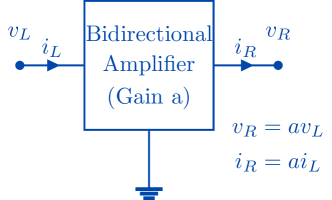
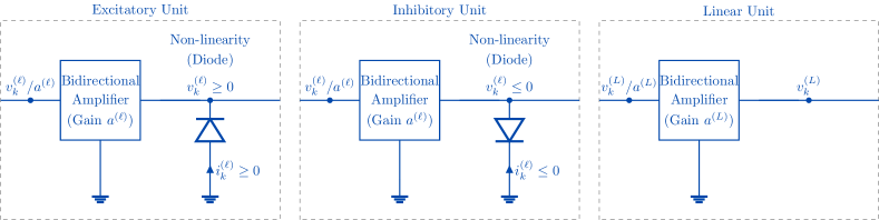
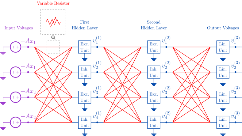
Figure 5: Top. Bidirectional amplifier with gain a. The right terminal voltage ($v_{R}$) is related to the left terminal voltage ($v_{L}$) by the relationship $v_{R}=av_{L}$, where $a$ is a gain factor. The left terminal current ($i_{L}$) is related to the right terminal current ($i_{R}$) by the relationship $i_{L}=\frac{1}{a}i_{R}$. Middle. A unit is composed of a bidirectional amplifier, possibly followed by a diode between the unit’s node and ground. Depending on the orientation of the diode, units come in two flavours: excitatory units and inhibitory units. Bottom. A deep resistive network with bidirectional amplifiers.

References

- Anisetti et al. (2022) Anisetti, V. R., Kandala, A., Scellier, B., and Schwarz, J. Frequency propagation: Multi-mechanism learning in nonlinear physical networks. arXiv preprint arXiv:2208.08862, 2022.
- Baez & Fong (2018) Baez, J. C. and Fong, B. A compositional framework for passive linear networks. Theory and Applications of Categories, 33(38):1158–1222, 2018.
- Dillavou et al. (2022) Dillavou, S., Stern, M., Liu, A. J., and Durian, D. J. Demonstration of decentralized physics-driven learning. Physical Review Applied, 18(1):014040, 2022.
- Dillavou et al. (2023) Dillavou, S., Beyer, B., Stern, M., Miskin, M. Z., Liu, A. J., and Durian, D. J. Circuits that train themselves: decentralized, physics-driven learning. In AI and Optical Data Sciences IV, volume 12438, pp. 115–117. SPIE, 2023.
- Hopfield (1984) Hopfield, J. J. Neurons with graded response have collective computational properties like those of two-state neurons. Proceedings of the national academy of sciences, 81(10):3088–3092, 1984.
- Keiter (2014) Keiter, E. Xyce: An open source spice engine, Mar 2014. URL https://nanohub.org/resources/20605.
- Kendall et al. (2020) Kendall, J., Pantone, R., Manickavasagam, K., Bengio, Y., and Scellier, B. Training end-to-end analog neural networks with equilibrium propagation. arXiv preprint arXiv:2006.01981, 2020.
- Kiraz et al. (2022) Kiraz, F. Z., Pham, D.-K. G., and Desgreys, P. Impacts of feedback current value and learning rate on equilibrium propagation performance. In 2022 20th IEEE Interregional NEWCAS Conference (NEWCAS), pp. 519–523. IEEE, 2022.
- Laborieux & Zenke (2022) Laborieux, A. and Zenke, F. Holomorphic equilibrium propagation computes exact gradients through finite size oscillations. Advances in Neural Information Processing Systems, 35:12950–12963, 2022.
- Laborieux et al. (2021) Laborieux, A., Ernoult, M., Scellier, B., Bengio, Y., Grollier, J., and Querlioz, D. Scaling equilibrium propagation to deep convnets by drastically reducing its gradient estimator bias. Frontiers in neuroscience, 15:129, 2021.
- LeCun et al. (1998) LeCun, Y., Bottou, L., Bengio, Y., and Haffner, P. Gradient-based learning applied to document recognition. Proceedings of the IEEE, 86(11):2278–2324, 1998.
- Lopez-Pastor & Marquardt (2023) Lopez-Pastor, V. and Marquardt, F. Self-learning machines based on hamiltonian echo backpropagation. Physical Review X, 13(3):031020, 2023.
- Marković et al. (2020) Marković, D., Mizrahi, A., Querlioz, D., and Grollier, J. Physics for neuromorphic computing. Nature Reviews Physics, 2(9):499–510, 2020.
- Millar (1951) Millar, W. Cxvi. some general theorems for non-linear systems possessing resistance. The London, Edinburgh, and Dublin Philosophical Magazine and Journal of Science, 42(333):1150–1160, 1951.
- Oh et al. (2023) Oh, S., An, J., Cho, S., Yoon, R., and Min, K.-S. Memristor crossbar circuits implementing equilibrium propagation for on-device learning. Micromachines, 14(7):1367, 2023.
- Onsager (1931) Onsager, L. Reciprocal relations in irreversible processes. ii. Physical review, 38(12):2265, 1931.
- Paszke et al. (2017) Paszke, A., Gross, S., Chintala, S., Chanan, G., Yang, E., DeVito, Z., Lin, Z., Desmaison, A., Antiga, L., and Lerer, A. Automatic differentiation in pytorch. 2017.
- Salakhutdinov & Hinton (2009) Salakhutdinov, R. and Hinton, G. Deep boltzmann machines. In Artificial intelligence and statistics, pp. 448–455. PMLR, 2009.
- Scellier (2021) Scellier, B. A deep learning theory for neural networks grounded in physics. PhD thesis, Université de Montréal, 2021.
- Scellier & Bengio (2017) Scellier, B. and Bengio, Y. Equilibrium propagation: Bridging the gap between energy-based models and backpropagation. Frontiers in computational neuroscience, 11:24, 2017.
- Scellier & Mishra (2023) Scellier, B. and Mishra, S. A universal approximation theorem for nonlinear resistive networks. arXiv preprint arXiv:2312.15063, 2023.
- Scellier et al. (2022) Scellier, B., Mishra, S., Bengio, Y., and Ollivier, Y. Agnostic physics-driven deep learning. arXiv preprint arXiv:2205.15021, 2022.
- Scellier et al. (2023) Scellier, B., Ernoult, M., Kendall, J., and Kumar, S. Energy-based learning algorithms for analog computing: a comparative study. In Thirty-seventh Conference on Neural Information Processing Systems, 2023.
- Stern & Murugan (2023) Stern, M. and Murugan, A. Learning without neurons in physical systems. Annual Review of Condensed Matter Physics, 14:417–441, 2023.
- Stern et al. (2022) Stern, M., Dillavou, S., Miskin, M. Z., Durian, D. J., and Liu, A. J. Physical learning beyond the quasistatic limit. Physical Review Research, 4(2):L022037, 2022.
- Stern et al. (2023) Stern, M., Dillavou, S., Jayaraman, D., Durian, D. J., and Liu, A. J. Physical learning of power-efficient solutions. arXiv preprint arXiv:2310.10437, 2023.
- Vogt et al. (2020) Vogt, H., Hendrix, M., and Nenzi, P. Ngspice (version 31), 2020. URL http://ngspice.sourceforge.net/docs/ngspice-manual.pdf.
- Watfa et al. (2023) Watfa, M., Garcia-Ortiz, A., and Sassatelli, G. Energy-based analog neural network framework. Frontiers in Computational Neuroscience, 17:1114651, 2023.
- Wright et al. (2022) Wright, L. G., Onodera, T., Stein, M. M., Wang, T., Schachter, D. T., Hu, Z., and McMahon, P. L. Deep physical neural networks trained with backpropagation. Nature, 601(7894):549–555, 2022.
- Wright (2015) Wright, S. J. Coordinate descent algorithms. Mathematical programming, 151(1):3–34, 2015.
- Wycoff et al. (2022) Wycoff, J. F., Dillavou, S., Stern, M., Liu, A. J., and Durian, D. J. Desynchronous learning in a physics-driven learning network. The Journal of Chemical Physics, 156(14), 2022.
- Xia & Yang (2019) Xia, Q. and Yang, J. J. Memristive crossbar arrays for brain-inspired computing. Nature materials, 18(4):309–323, 2019.
- Yi et al. (2023) Yi, S.-i., Kendall, J. D., Williams, R. S., and Kumar, S. Activity-difference training of deep neural networks using memristor crossbars. Nature Electronics, 6(1):45–51, 2023.