École Polytechnique, France and University of Warsaw, Poland CNRS, LaBRI, Université of Bordeaux, France and University of Warsaw, Poland CNRS, LaBRI, Université of Bordeaux, France \CopyrightG. Shabadi, N. Fijalkow, and T. Matricon {CCSXML} <ccs2012> <concept> <concept_id>10003752.10003790.10002990</concept_id> <concept_desc>Theory of computation Logic and verification</concept_desc> <concept_significance>500</concept_significance> </concept> <concept> <concept_id>10003752.10003790.10003806</concept_id> <concept_desc>Theory of computation Programming logic</concept_desc> <concept_significance>300</concept_significance> </concept> <concept> <concept_id>10010147.10010257.10010258.10010261</concept_id> <concept_desc>Computing methodologies Reinforcement learning</concept_desc> <concept_significance>500</concept_significance> </concept> </ccs2012> \ccsdesc[500]Theory of computation Logic and verification \ccsdesc[300]Theory of computation Programming logic \ccsdesc[500]Computing methodologies Reinforcement learning \EventEditorsJohn Q. Open and Joan R. Access \EventNoEds2 \EventLongTitle42nd Conference on Very Important Topics (CVIT 2016) \EventShortTitleCVIT 2016 \EventAcronymCVIT \EventYear2016 \EventDateDecember 24–27, 2016 \EventLocationLittle Whinging, United Kingdom \EventLogo \SeriesVolume42 \ArticleNo23
Theoretical foundations for programmatic reinforcement learning
Abstract
The field of Reinforcement Learning (RL) is concerned with algorithms for learning optimal policies in unknown stochastic environments. Programmatic RL studies representations of policies as programs, meaning involving higher order constructs such as control loops. Despite attracting a lot of attention at the intersection of the machine learning and formal methods communities, very little is known on the theoretical front about programmatic RL: what are good classes of programmatic policies? How large are optimal programmatic policies? How can we learn them? The goal of this paper is to give first answers to these questions, initiating a theoretical study of programmatic RL.
keywords:
Reinforcement learning, Markov decision processes, Program synthesiscategory:
\relatedversion1 Introduction
Reinforcement learning (RL) is a very popular and successful field of machine learning where the agent learns a policy in an unknown environment through numerical rewards, modelled as a Markov decision process (MDP). In the tabular setting, the environment is given explicitly, which implies that typically policies are also represented explicitly, meaning as functions mapping each state to an action (or distribution of actions). Such representation becomes quickly intractable when the environment is large and makes it hard to compose policies or reason about them. In the general setting the typical assumption is that the environment can be simulated as a black-box. Deep reinforcement learning algorithms which learn policies in the form of large neural networks have been scaled to achieve expert-level performance in complex board and video games [18, 23]. However, they suffer from the same drawbacks as neural networks which means that the learned policies are vulnerable to adversarial attacks [17] and do not generalize to novel scenarios [19]. Moreover, big neural networks are very hard to interpret and their verification is computationally infeasible.
To alleviate these pitfalls, a growing body of work has emerged which aims to learn policies in the form of programs [22, 4, 21, 24, 10, 12, 20, 16, 2, 13], under the name “programmatic reinforcement learning”. Programmatic policies can provide concise representations of policies which would be easier to read, interpret, and verify. Furthermore, their short size compared to neural networks would mean that they can also generalize well to out-of-training situations while also smoothing out erratic behaviors. The goal of the line of work we initiate here is to lay the theoretical foundations for programmatic reinforcement learning.
All the works cited above use very simple programming languages, combining finite state machines, decision trees, and Partial Integral Derivate (PID) controllers (originating from control theory). We believe – and show evidence in this work – that more expressive programming languages can help describing policies succinctly and naturally. The fundamental question we ask is:
Given a class of environments, how to define a class of programmatic policies such that for each environment in , there exists an optimal111Different notions of optimality can be considered here. programmatic policy .
We call such statements “expressivity results”. The design of is a compromise, since the class should be rich enough to express optimal policies, but simple enough to meet the objectives stated above: readable, interpretable, verifiable, generalizable, as well as learnable. There are actually many instances of expressivity results originating from different fields:
- •
- •
-
•
In automatic control, PID controllers [3] form a very classical and versatile class of programmatic controllers widely used in practice for continuous systems.
-
•
In machine learning, the fact that neural networks are universal approximators implies that neural networks can be used as (approximate) policies for general reinforcement learning tasks.
Once existence is understood, one can wonder about sizes: how large are optimal programmatic policies? We refer to results placing upper and lower bounds on sizes of optimal programmatic policies as “succinctness results”.
To define classes of environments we use a simple but versatile programming language: (an idealised version of) PRISM, which is at the heart of the most successful probabilistic model checkers (PRISM [11] and STORM [9]). The technical contribution of this work is to prove expressivity and succinctness results for a subclass of the PRISM language, consisting of two dimensional deterministic grids. We construct a very simple and elegant class of programmatic policies in the form of sequences of subgoals, inspired by Shannon’s early experiments on mechanical mice. Our main result is obtained through geometrical insights into the corresponding class of environments. To the best of our knowledge, this is the first example of a non-trivial programming language, employing at its heart control loops, which can express small optimal policies on a large class of environments.
2 A framework for programmatic reinforcement learning
For simplicity, the environments we consider are discrete-time MDPs. The definitions we give here and the questions we ask can be naturally extended to more complicated environments, using for instance rewards functions or continuous time.
Definition 2.1 (MDP).
A markov decision process (MDP) is a tuple where is a set of states, is a finite set of actions, is the transition function mapping a state and an action to a probability distribution over the state space, and is the initial state.
We refer to [15] for the classical definitions (probabilistic space, policies, optimal policies). An MDP can be regarded as an environment in which an agent observes the current state of the game and picks an action to take following which the game updates the state using the transition function. Before presenting the PRISM syntax, let us consider the following example.
Example 2.2.
The following codeblock defines an MDP in PRISM syntax222We deviate from PRISM syntax in cosmetic ways. PRISM supports specifying a wider range of stochastic models, for instance reward models for MDPs..
The MDP specified here contains two state variables x,y which take integer values ranging from to . The initial state is (0,0). The MDP contains two regions which are specified by the predicates: x < 10 && x + y >= 2 and x < 10 && 3*x - y <= 20. In the states where the first predicate is satisfied, two actions up and down are enabled. If in one of these states and the up action is picked by the agent, with probability the next state is obtained by incrementing the -coordinate by 1 and with probability both and are incremented.
We define now the idealised PRISM syntax. The state space is described by tuples of discrete variables. Each variable is specified by
where are integers and . The rest of the program consists in a set of commands of the form
where is an action, are states, is a predicate on states, is the update function computing the next state, and . The interpretation is as follows: from any state satisfying , the action is available, and its effect is a random event: with probability we move to state . In this idealised definition predicates and update functions are not restricted in any way (they should be at the very least computable). We call environment programs the class of environments defined by such programs, and happily identify programs and the environments they define.
The point of PRISM programs is that the use of predicates and update functions enable partitioning the state space into regions which have similar transitions, leading to very concise representations of large MDPs. For instance, the MDP given in the example above has states, but is given by lines of code.
Finally, we consider a specification, such as reaching a target state almost surely; we then say that a policy is optimal if it satisfies the specification. We can now formulate the problem we study in this work in a very precise manner:
Given a subclass of PRISM programs , define a class of programmatic policies such that for each MDP definable by , there exists an optimal policy given by some program .
3 Two dimensional deterministic gridworlds with linear predicates
PRISM programs as we defined them above can have extremely complex behaviours; for instance, it is very easy to write a PRISM program illustrating Collatz conjecture:
It is conjectured that for any initial state , for large enough, the unique path eventually reaches , but the proof of this conjecture has eluded mathematicians for decades. Therefore, we will now focus our attention on a simple subclass of PRISM programs, which will be rich enough to include complicated behaviours, yet tamed enough to admit non-trivial expressivity and succinctness results. The restrictions are:
-
•
There are state variables in , where is a parameter.
-
•
There are actions, which represent the cardinal directions of , and DOWN corresponding to the updates , and respectively.
-
•
The predicates are all conjunctions of linear predicates, meaning .
We call LINGRID this class of environment programs. The linear predicates partition the grid into convex polygonal regions, which we refer to later as the regions, see Figure 1. Note that an instance of LINGRID with parameter as exactly many states. The number of regions may be much smaller, it is linear in the size of the environment program. The goal of this work will be to show that we can represent policies whose size depend only on the number of regions, and not on the parameter .
Let us make a cosmetic yet important assumption: we work in a continuous relaxation of the environment, where from a state the agent can choose any convex combination of the available actions, leading to an edge of the current region. The discrete and continuous semantics are equivalent when choosing a small enough granularity for discretization: the continuous relaxation is very reasonable and it enables geometric reasoning.
We consider reachability objectives, where the goal is to reach a target region. Since the environments are deterministic, this means finding a path from the initial state to the target. In other words, an optimal policy is a path to the target region. Thus, we will be using path and policy interchangeably moving forward.
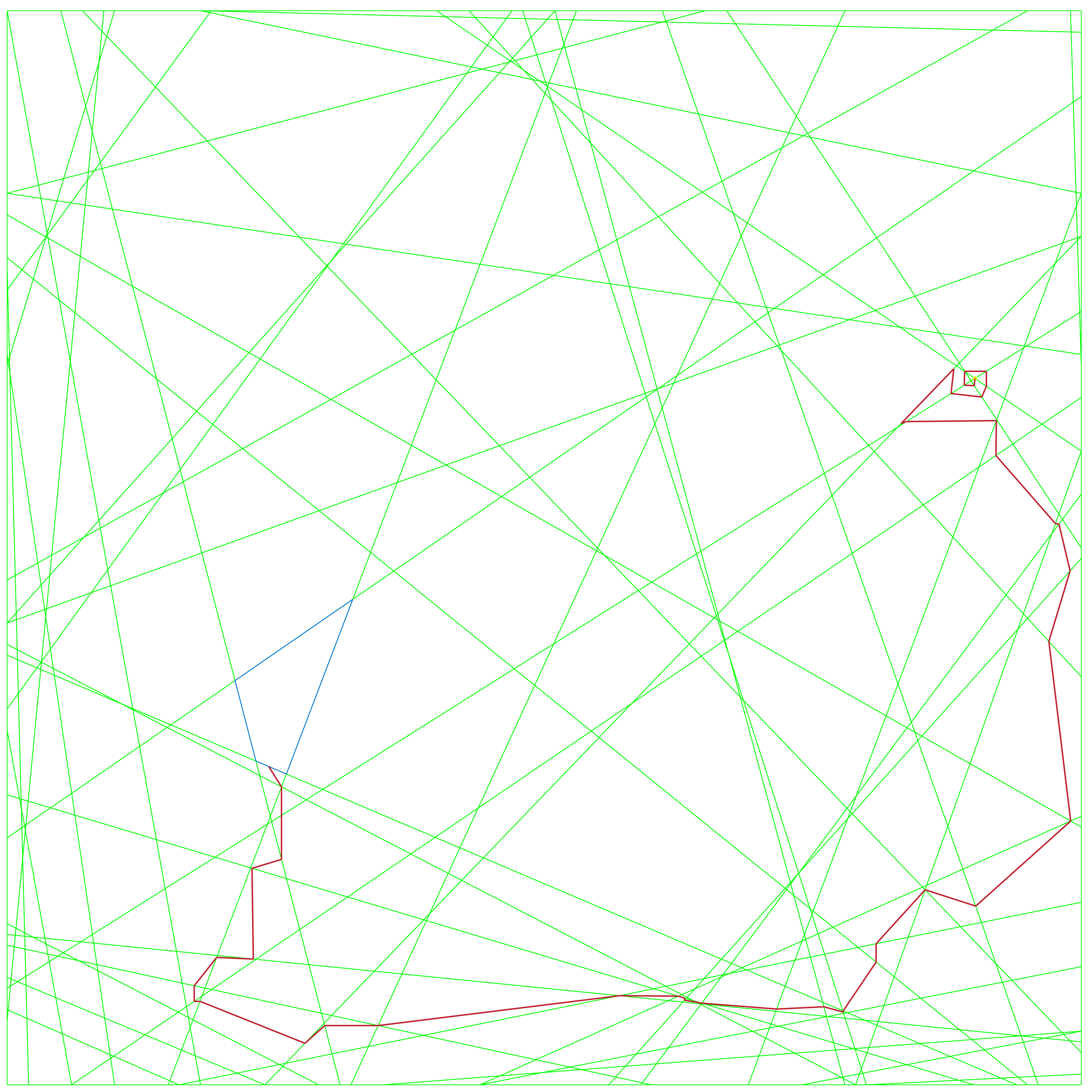
Example 3.1 (Spiral).
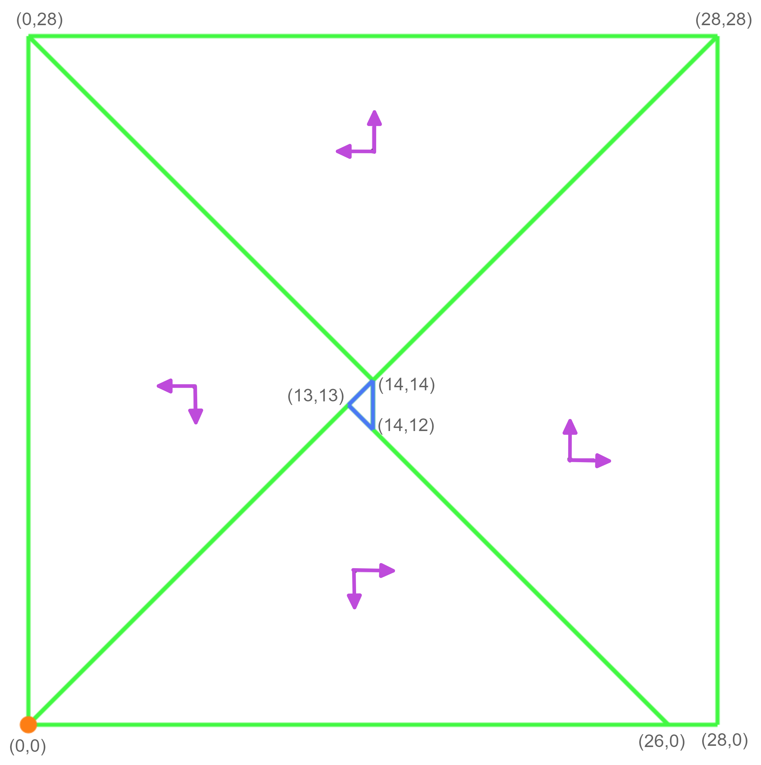
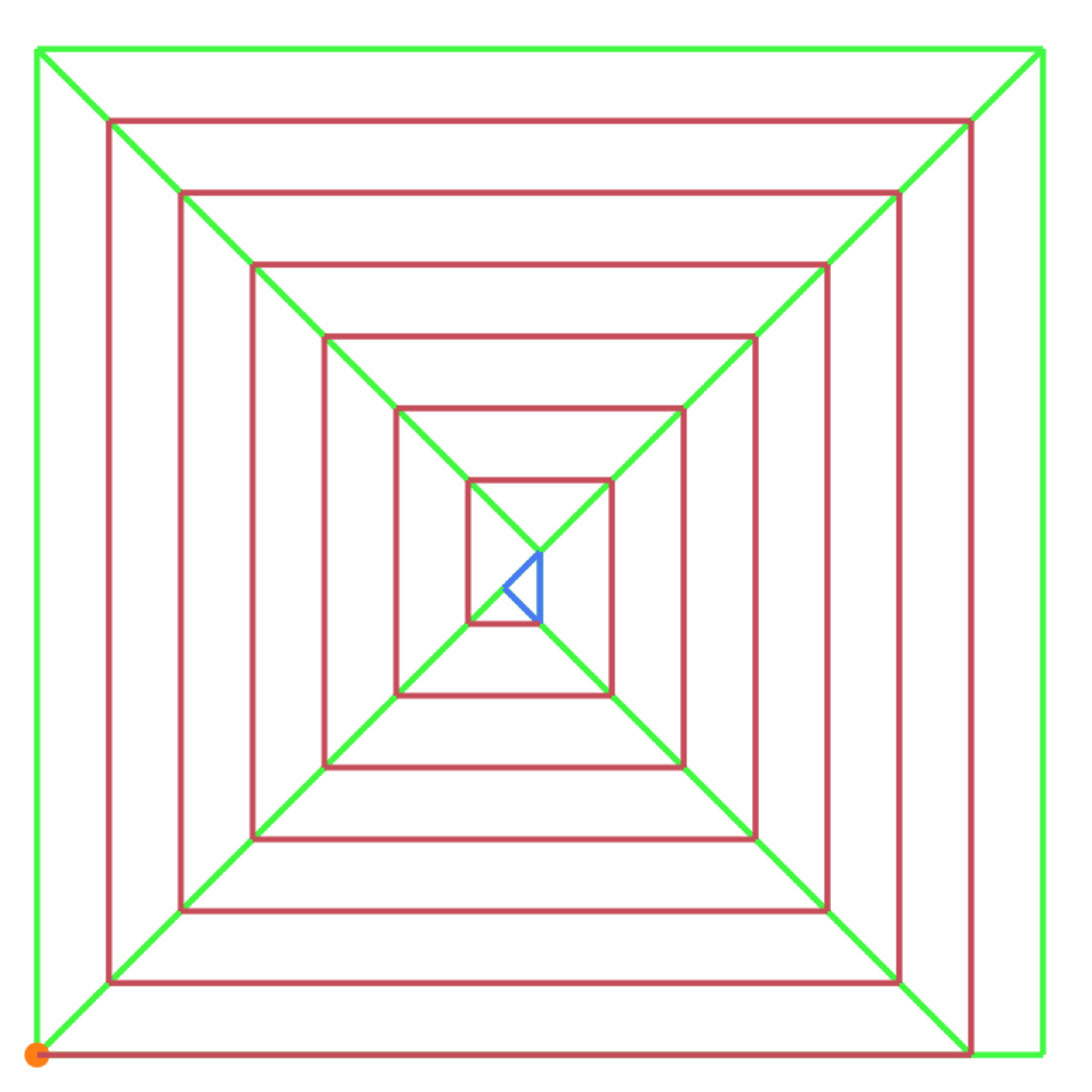
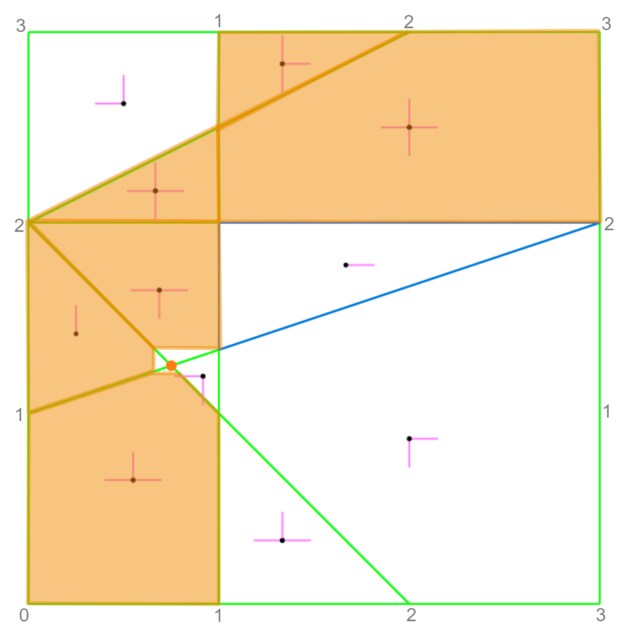
In Figure 1(a) we have an example of an instance of LINGRID. The state space is a grid and there are regions with the allowed actions in the regions indicated by arrows within the region. The initial state (in orange) is and the target region is the triangular region in the middle. Figure 1(b) visualizes the path from the initial state to the target region, looping around it. The length of the path is proportional to the state space; extrapolating, it is in an grid. But the path is very regular, which indicates that we should be able to have a compact representation: by the end of this paper, we will construct a programmatic representation whose size depends on the number of regions but is independent of .
To reason with gridworlds we need precise terminology and notations. States are pairs . For any , we define the segment to be the set of points connecting and . We let Regions denote the set of regions, which are closed convex polygons, and denote the set of actions available in region . We say that there exists a move between and if they belong to the same region and is in the convex hull of seen as unitary vectors , and . By extension, there exists a path from to if there exists a sequence of consecutive moves starting in and ending in . For a region , we use to refer to the set of edges of . Note that edges are segments, but when introducing an edge we implicitely mean the edge of some region. Since each edge is shared by at most two regions, we can define to be the region adjacent to which both share the edge on their boundaries. However, since some edges lie on the boundaries of the grid , might not exist.
4 The tree of the winning region
The first direction we explore while searching for concise representations of policies is region based policies where the policy picks a single action per region. For example, with the spiral gridworld from Example 3.1, it is sufficient to pick one action per region to navigate the agent from the initial state to the target region. However, this is not the case in general, as shown in the following example.
Example 4.1 (Double pass triangle).
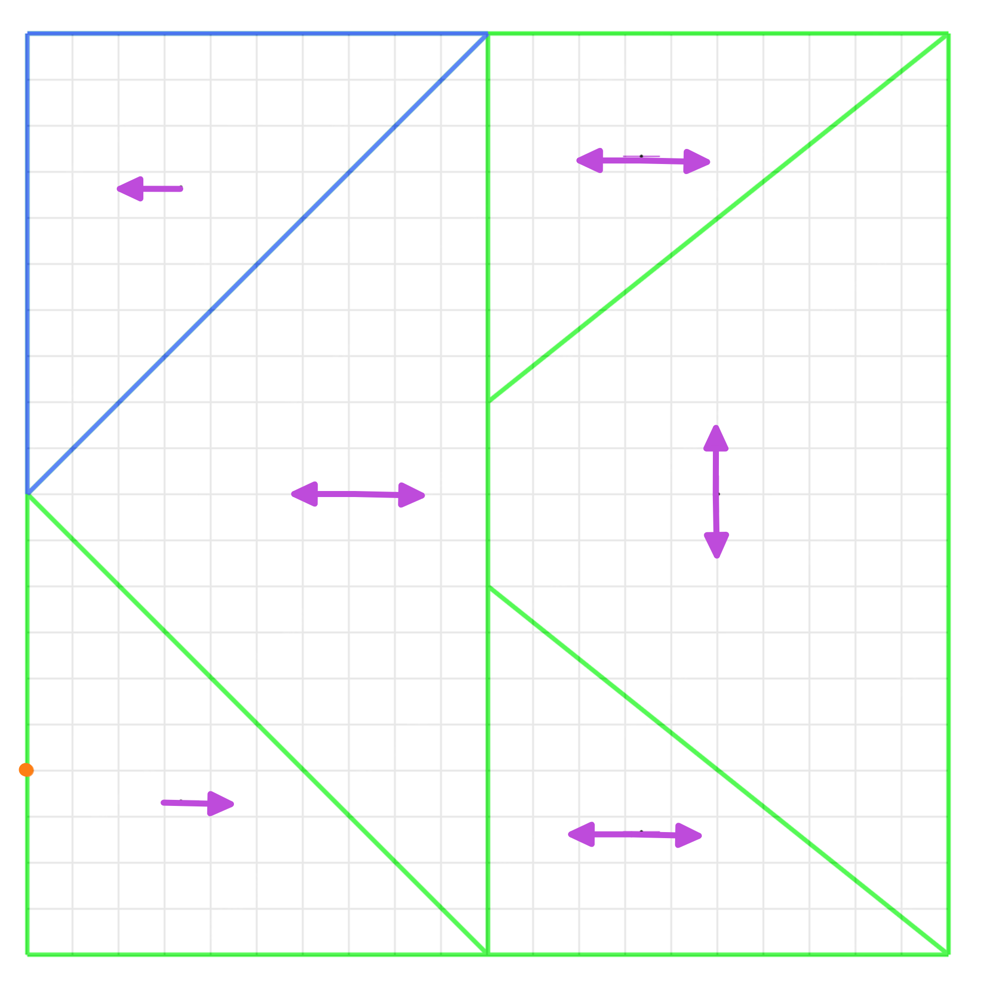
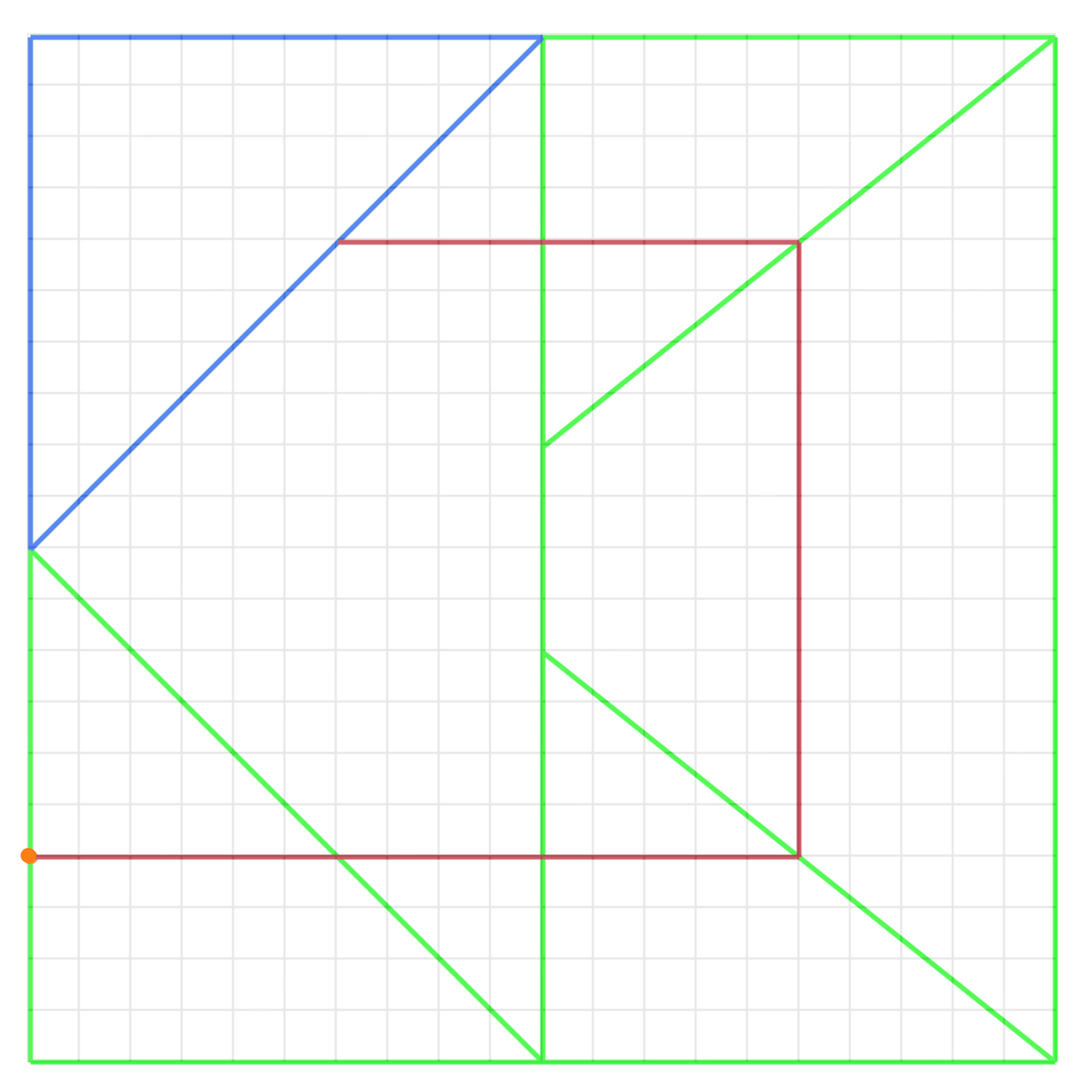
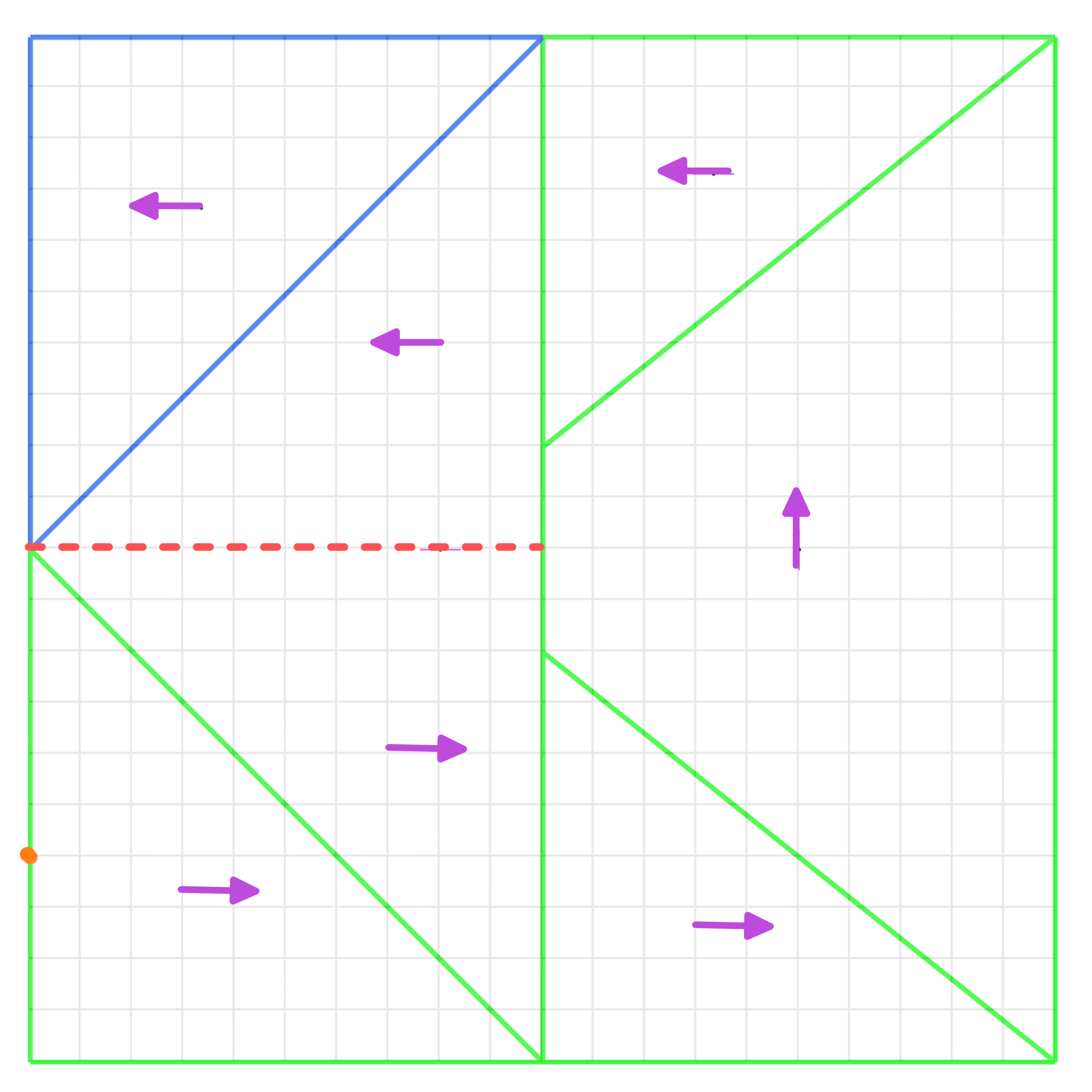
In Figure 2(a), we have an example of an instance of LINGRID. Figure 2(b) visualizes the path from the initial state to the target region. The important remark here is that the triangular region in the middle is crossed twice, with different actions: first time right, second time left. It is very tempting to refine this region as shown in Figure 2(c) to obtain a region-based policy: this is what we will be doing next!
As a tool for reasoning on paths we construct an algorithm computing the set of winning states, meaning for which there exists a path to the target region. At a high-level, the algorithm is a generic backward breadth-first search algorithm: starting from the target region, it builds and expands a tree where the nodes represent states that can reach the target. Taking advantage of the convexity assumption (that we can play any convex combination of available actions), we show that we only need to reason with segments included in edges of the regions.
The backward algorithm builds a tree as follows. The root is a special node, whose children are all the edges of the target region . Nodes are pairs consisting of a segment and a region such that . To expand a node , we identify the region sharing with , if it exists. We then consider the set of states of for which there exists a move to a state in : it is the convex combination of segments included in the edges of . For each such segment , we remove from it all segments already appearing in a node of the tree, and if the segment it yields is non-empty, then we add a node as a child of the node .
Example 4.2.
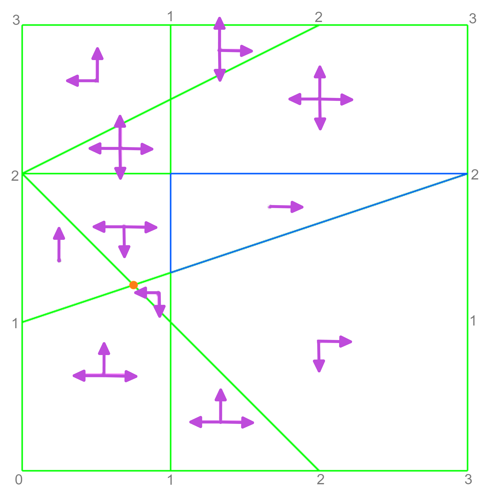
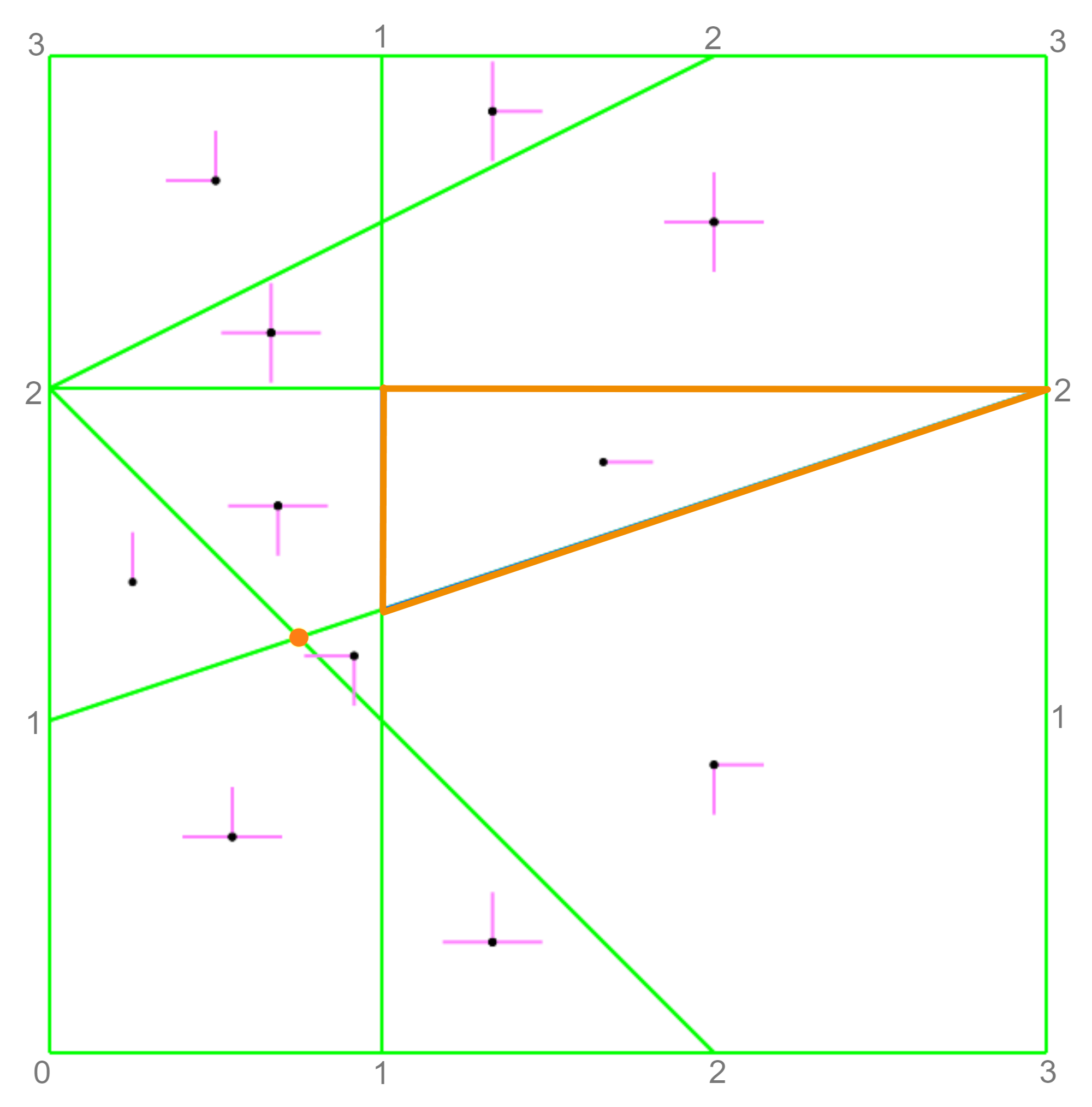
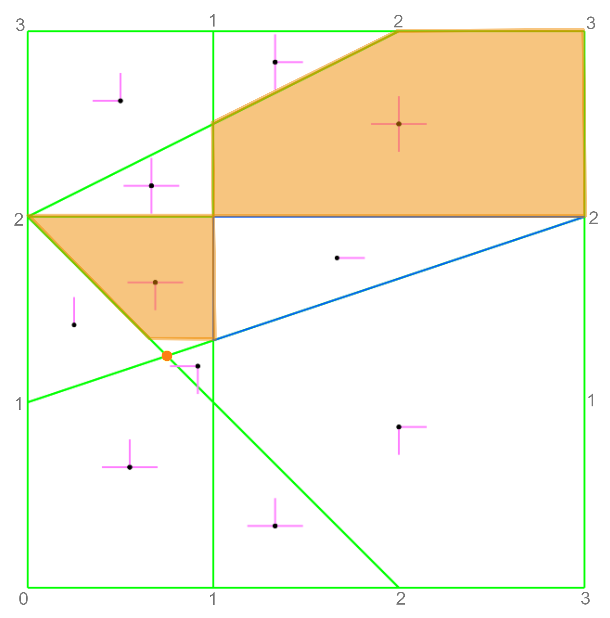
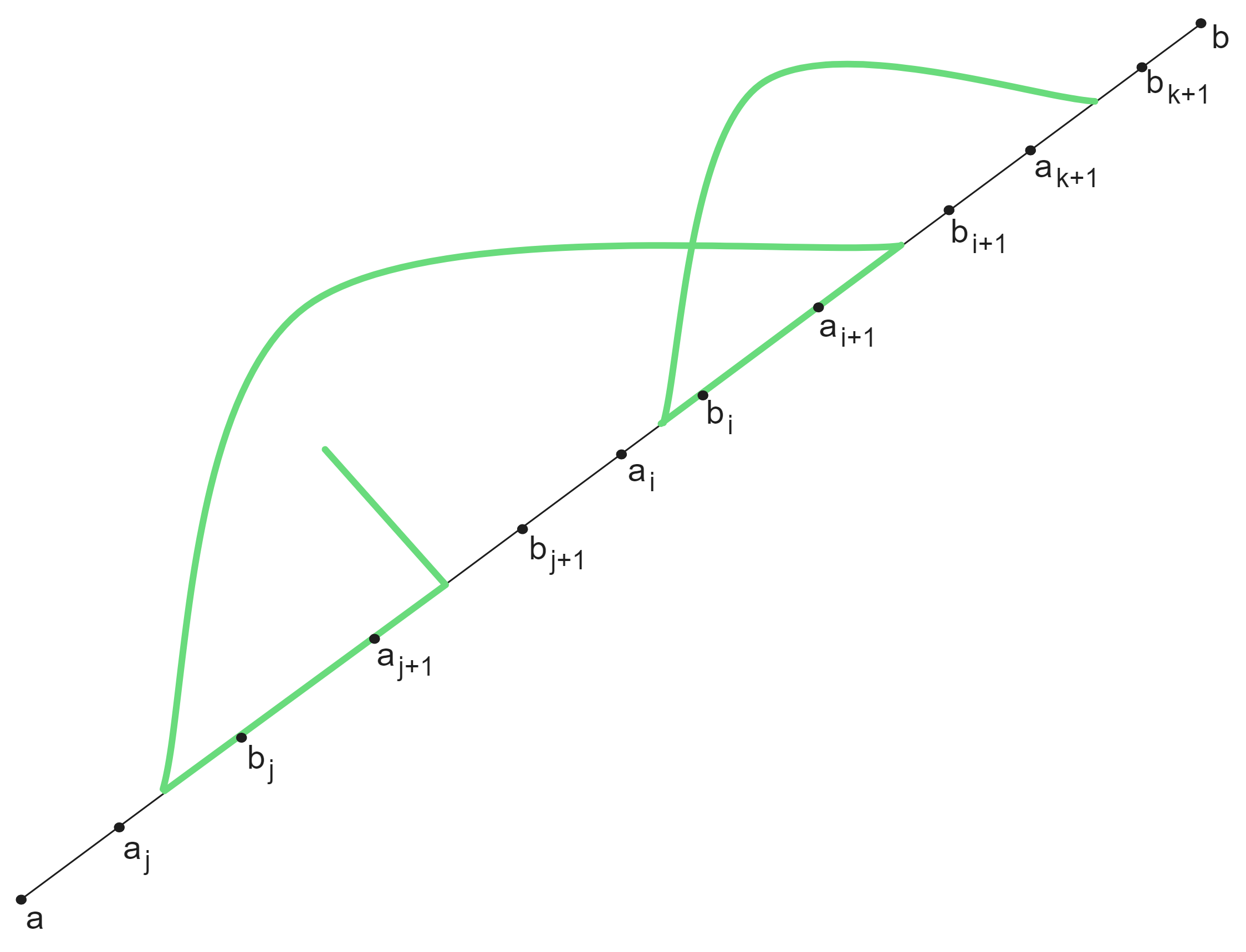
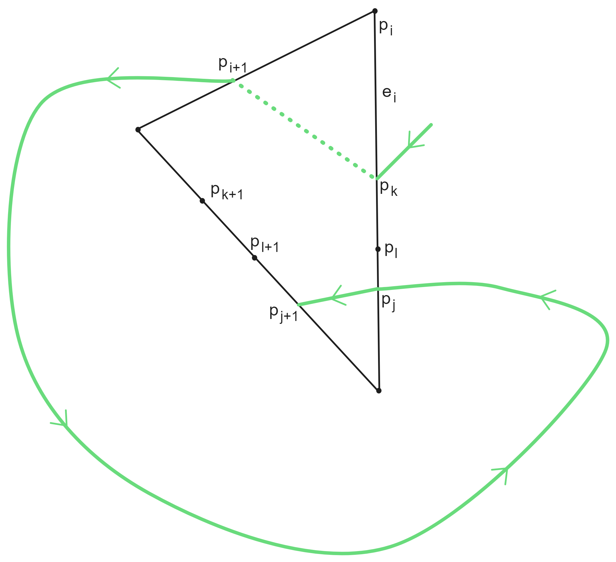
In Figure 3, we can visualize how the backward algorithm works. The tree itself can be seen in Figure 4. We represent 3 subtrees, each corresponding to an edge of the target region. Starting from these 3 edges, we add segments of edges of adjacent regions as nodes to the trees in a breadth-first manner. There exists a path from each state in a node to a state in its parent node.
By construction, from each state in a segment of a node of the tree we can construct a path to the target region. Conversely, every state on an edge for which there exists a path to the target region belongs to some node of the tree. Since there might be more than one state in its parent segment that is reachable, the tree represents a family of paths to the target region. Importantly, these paths never visit the same point twice: they are non self-intersecting. This is due to how we have constructed the tree, filtering out parts of segments which we have already visited.
We are far from done: at this point, the paths we obtained do not have a compact programmatic representation. In particular, their lengths can only be bounded as a function , parameter determining the size of the environment. A lot more geometrical insights into the gridworld environments will be necessary to succinctly represent policies.
5 The class of policy programs
5.1 Inspiration
In 1950, Claude Shannon built, as a small project at home, one of the first instances of machine learning that the world had witnessed: a mechanical mouse capable of learning to solve a configurable maze in which the maze walls could be positioned as desired333https://www.technologyreview.com/2018/12/19/138508/mighty-mouse/. To do this, he repurposed telephone relay circuits and placed them underneath the maze board to navigate the mouse towards the exit. In a first pass, the mouse would systematically explore the whole maze looking for the exit and learn the path, so that in its subsequent attempts, it could swiftly reach the target. The magic was hidden in the relay circuits which would remember the path and were able to tell the mouse to turn left or right based on whether a switch was on or off. The first attempt is reminiscent of reinforcement learning with a trial and error approach to learn a policy to solve the game. However, our focus in this work will be on the subsequent attempts where we observe a programmatic abstraction to obtain a concise representation of the policy: instead of specifying the direction to follow at each point of the maze, the relay switches only indicated the points at which to change direction.


5.2 Programmatic policies
Before defining the programming language, let us dive into an example.
Example 5.1.
The following code block contains a programmatic policy for the spiral example given in Example 3.1.
This program ensures to reach the segment , which is an edge of the target region. To do this, it specifies moves starting from four segments: , , , and . Figure 1(a) can help visualize these segments: this is the four diagonals. From we have two target segments: if we can reach , then we do (indeed this is part of the target region so we are done), otherwise we aim at . Importantly, when aiming at we want to go as close as possible to as specified by the preference. Here this means choosing only action RIGHT, and not DOWN. In the other three segments there is a single target segment.
In general, a policy program is a sequence of Do Until loops:
This is interpreted as: run the local program until reaching the edge , which we call the local goal. A local program is a set of instructions of the form
where are segments and vertices, with an extremal point of . It is interpreted as: from any state in the segment , let be the least index such that there is a move from to ; move to the reachable state of closest to . We also allow the possibility of simply specifying a direction to follow in instead of a target and a preference.
6 Properties of the tree of the winning region
In this section we will prove properties of paths in gridworlds environment. These are preliminary steps before constructing an algorithm deriving programmatic policies from paths. A branch of the tree of the winning region is a sequence of segments
The branch induces a sequence of pairs of regions and edges . For each : (i) the moves between and are contained in , (ii) , (iii) , (iv) , and (v) .
Lemma 6.1.
There exist at most two indices such that and .
Proof 6.2.
Arguing by contradiction, suppose there exist 3 indices such that and and . Let us denote the common edge by the segment and without loss of generality, assume for each of the segments , , , , , and , the first vertex of the segment is closer to and the second vertex is closer to . This orientation makes the following arguments easier.
In the rest of the proof, we base our arguments on the algorithm used to construct the tree of the winning region. First, let us place ourselves in the situation when the leaf associated to the segment was being extended. is a segment from which there exists a path to . As we filter out parts of edges which have already been explored, either or . So assume . Then, in fact we have a path from each point in to . This is due to the fact that there exists such that is included in the cone of actions allowed in . As for each , is along the same direction as , it is also in the cone of allowed actions. Thus, the whole segment has been explored until now.
The next time we visit this edge, we have that . Similar to before, since has been explored or . Suppose we are in the former case. So has been explored and thus . Now, one can see in Figure 6 that any path represented by the segments, which visits is necessarily self intersecting. Note that here we assumed and , but each of the three other cases can be verified similarly that they all give us self intersecting paths.
Lemma 6.3.
Assume there exist indices such that , and contains at least two orthogonal directions. Then,
-
1.
if the sequence of segments forms an inner loop at , then all the edges of regions inside the loop are not visited by the subsequence .
-
2.
if the sequence of segments forms an outer loop at , then all the edges of regions outside the loop are not visited by the subsequence .
-
3.
if is the least index such that and , we can construct from and such that and each point in is reachable from a point in .
Proof 6.4.
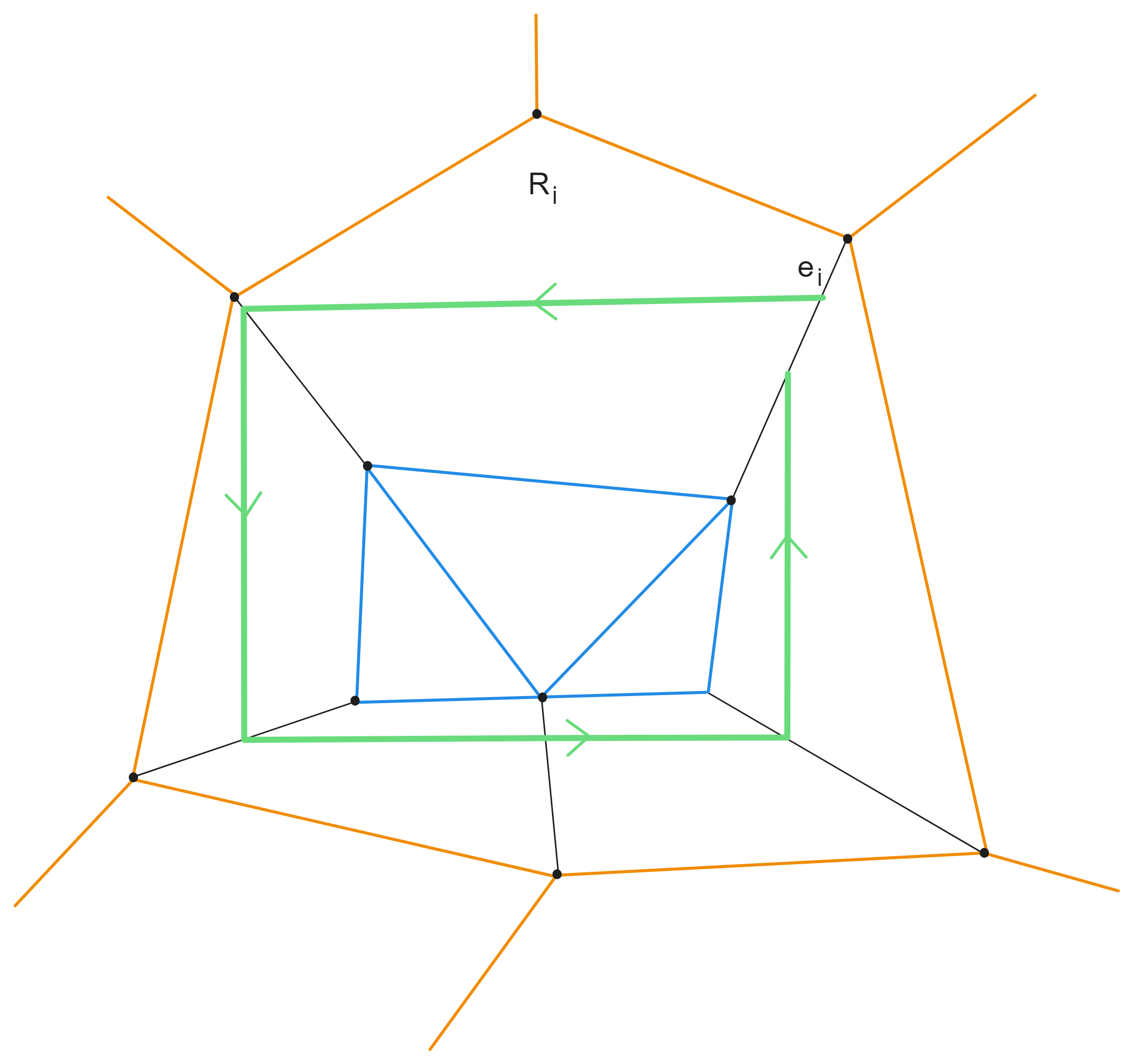
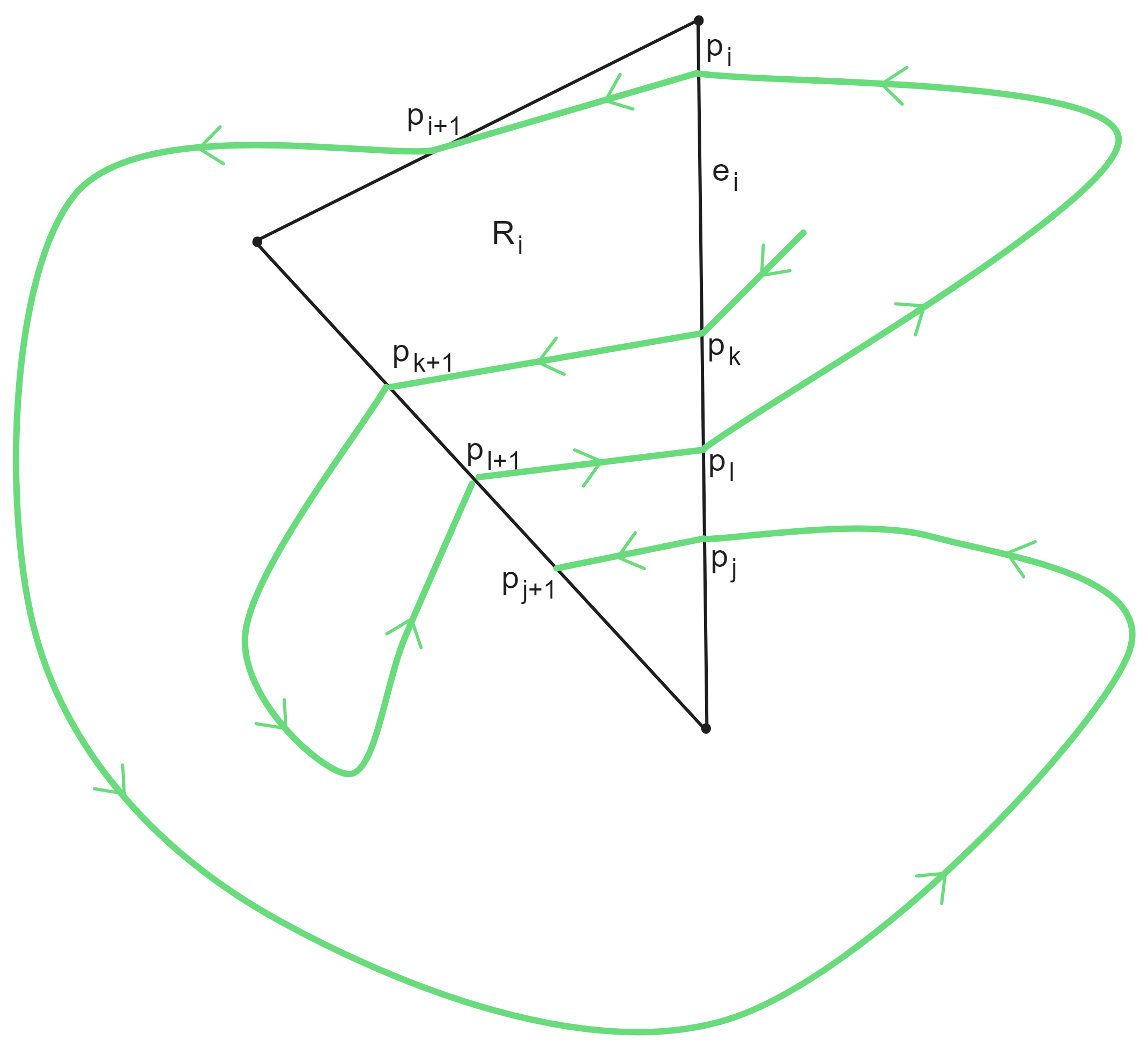
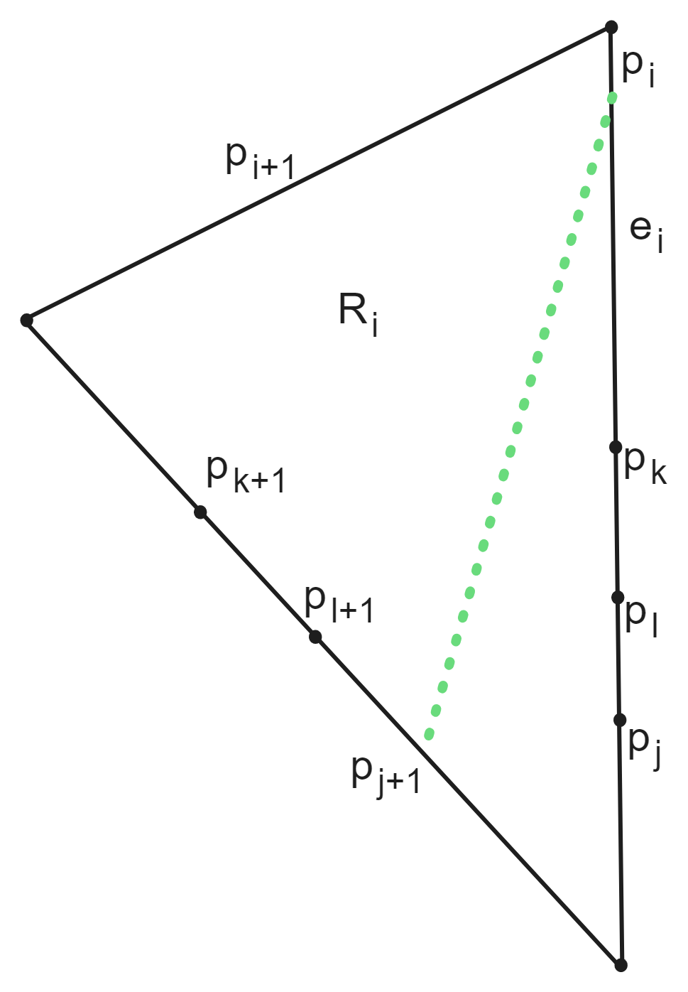
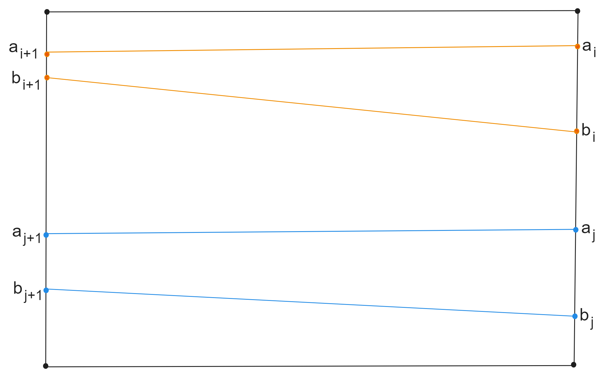
Let us begin by understanding what we mean by a loop and edges being inside and outside loops. Looking at Figure 7(a), the path (in green) starting at forms a loop at this edge. As soon as this loop is completed, the edges of regions not involved in the loop are partitioned into disjoint two sets: the edges inside the loop (in blue) and those outside (in orange). It is important that else the loop of edges would not be formed.
We will now prove item 1, the proof of item 2 follows a similar pattern. To this end, we again proceed by contradiction and assume that we have a sequence of segments which visits an inner edge before forming a loop at . Let . There exists a path going from to . Now take a look at Figure 7(b) in which we can see a loop being formed by the path from to . If this sequence of segments visits an inner edge before forming the loop, it has to pass through the space in the edge between and because if not, we would have a self intersecting path. Thus, there exist indices such that which are the indices where the sequence enters and exits the edge while visiting an inner edge. Let and consider a path visiting which can also be seen in Figure 7(b).
Since , without loss of generality, we assume that as seen in the figure. Using the assumption that we have at least two orthogonal directions allowed in , we have two cases: or . In the first case, would be reachable from and (see Figure 7(c)) and so this segment would have been explored while the node was being extended which means that cannot exist in the space between and . Similarly in the second case, if , would be reachable from and (see Figure 7(d)) and therefore for the same reasons, cannot exist above . This concludes the proof of item 1.
Moving on to proving item 3, let us denote by for . Same as before, let us assume without loss of generality that and . This can be visualized through Figure 8. As at least two orthogonal directions are allowed in , let us again split into two cases with the first one being . Firstly, is below as seen in the figure because if not, (which would also have to be above to avoid self intersecting paths) would be reachable from so it would have already been explored at index and cannot exist there at index . By assumption, as is the least such index satisfying the property, using arguments similar to the previous part of the proof, we have that there is no index such that . This means that when the tree node associated to the segment was being extended, was unexplored. Also, we have that , otherwise would be reachable from . Thus necessarily, , i.e., lies on the same -coordinate as . As a result, we can determine simply by intersecting the line with the region . Lastly, , i.e., lies below and therefore we can set (which can be computed) and to be other point on the edge of on the same -coordinate as . We remark that there is a path from each point in to : just go left! Symmetric arguments can be used to deal with the case in which .
7 Constructing policy programs
What remains to be done is derive from a path a programmatic policy; one could say “compress” a path. This is the purpose of Algorithm 1. Lemma 6.3 provides the main idea for the construction of the policy synthesis procedure. As we have shown, whenever a loop is formed by the path, a new edge is discovered as soon as the loop is exited due to the non self-intersecting property. This motivates us to consider programmatic policies with a sequence of Do Until blocks corresponding to the sequence of edges in the order in which they are discovered by a path.
The algorithm works as follows: it takes in a sequence of segments from a tree of the winning region and the corresponding sequence of edges . It goes through both these sequences and each time a new edge is encountered, it begins a new Do Until block. At each iteration of the loop, if it sees that a segment of the next edge is already a target, i.e., if it visits the same pair of consecutive edges twice, it merges the two segments. This merging procedure ensures that when we encounter a loop in our path, segments belonging to the same edge are merged thus resulting in a compact representation of the sequence of segments. When we merge, we also set the preference depending on which side the next segment is with respect to the previous segment on the same edge. Intuitively, this allows to distinguish between inner and outer loops where the preference would force the policy to navigate towards a certain extreme of a segment thereby allowing the agent to progress closer towards the target region. The regions in which the allowed actions are a subset of or are handled differently by the algorithm. Since diagonal directions are not allowed in such regions, it suffices to specify the direction in which to navigate.
We now shift our attention to proving the correctness of Algorithm 1, which means proving an expressivity result, given by Theorem 7.1 and a succinctness result in the form of an upper bound on the size of the synthesized programmatic policies, in Theorem 7.3.
Theorem 7.1.
Given the shortest sequence of segments in the tree of the winning region going from the initial state to the target region, Algorithm 1 synthesizes a programmatic policy that can navigate an agent through these segments.
Proof 7.2.
We will show that the synthesized policy navigates an agent through the sequence of segments in the same order. Arguing by induction, it suffices to show that if the agent is currently at a point for some , the policy would guide the agent towards a point . When the agent is at , the execution of the program would be in a certain Do Until block. Firstly, we argue that the edge that contains contains at least one target in its From instruction in the current block. This is true by construction because the synthesis algorithm processes each segment sequentially and as a result each edge that appears in the sequence would have an associated From instruction. Note that the only case when this would be untrue is when the goal of the Do Until block is reached in which case the program execution would switch to the next block.
Next, within a From instruction, there may be several target segments separated by Else statements. Again, by construction, at least one of them is reachable from . Furthermore, the first reachable target segment contains because if not, this target segment (which would appear at index greater than ) would be reachable from . Consequently, we would have a shorter sequence of segments leading to a contradiction.
Lastly, it remains to prove that the policy would indeed navigate to a point in . Here, we need to distinguish two cases. In the first case, suppose that the target segment in the From instruction was formed without any merging of segments. Then necessarily the target segment coincides with or it is a region in which the allowed actions are a subset of or . Both the scenarios are easily handled. The interesting case is when the target segment was formed by the merging of segments. It means that the edge was visited twice and we have a loop at . This is where the Preference plays a role in navigating the agent in the correct direction. Note that at least two orthogonal actions allowed in . As we noted in the proof of Lemma 6.3, when we enter a loop in such a region, the segment has the same or coordinates as depending on the actions allowed. This means that there is a point with the same or coordinate as in the target segment. By taking another look at Figure 8, we can further see that coincides with the point reachable in the target segment that is extremal with respect to the Preference. Here, the synthesized merged segment would be with Preference: . If the agent is at a point in , and the allowed actions are UP and LEFT, the policy would navigate the agent towards a point in with the same -coordinate (i.e., go LEFT) because that would be the point that is extremal with respect to the specified Preference.
Theorem 7.3.
Given the shortest sequence of segments in a tree of the winning region going from the initial state to the target region, Algorithm 1 synthesizes a programmatic policy of length at most .
Proof 7.4.
Firstly, we remark that as we have at most edges in the gridworld, we have at most blocks Do Until representing the subgoals. Suppose that the sequence of segments visits unique edges and let denote the sequence of these edges in the order that they are first visited. Each of these correspond to a Do Until block in the policy.
Let us now analyse the size of each Do Until block which corresponds to a programmatic representation of a part of the sequence of segments going from to for a certain . Let denote this sequence of segments which forms a part of the sequence . Note that and are segments within the edges and respectively. Also, keep in mind the sequence of pairs of regions and edges traversed by the sequence which will be useful in the rest of the proof.
Observe that each unique edge in is associated with a From instruction within the Do Until block. As a first step, let us treat the indices such that . By Lemma 6.1, this happens at most twice with so this contributes at most two targets, and thereby two lines to the From instruction of . On the other hand, suppose . As a first subcase, suppose or . From Algorithm 1 it is clear that such regions would add at most two targets (directions) to the From instruction. Next assume at least two orthogonal directions are allowed in . If at most once with , then it contributes only one target to the From instruction. However, if there is another index such that and , by Lemma 6.3, it means that we have an inner or an outer loop. From this case, we would again have at most two targets: either and so the target segments would be merged (and the loop continues) or is a new edge never visited before (and the loop is exited). In other words, a loop contributes at most two target segments to each edge and there is at most one loop in a Do Until block.
In total, we have at most six targets associated with each edge in the Do Until block. Since only edges are explored by the -th block, each block has at most instructions. Thus, we obtain the following bound on the total length of the policy
| (1) |
In Theorem 7.3, we made the assumption that each segment in the sequence can be stored in constant space. This would imply that we can store rationals of arbitrary precision representing the endpoints of the segments in constant space. Obviously, this is not a valid assumption in practice and in the case where all the edges of the regions are described by rationals, we prove the following upper bound on the space required to store the segments.
Lemma 7.5.
Suppose there exists such that each of the endpoints of each of the edges of the regions are of the form for some , then each segment of a path of the tree of the winning region can be stored in space at most when both and can be written in the same form.
Proof 7.6.
Let
be an edge of a region in Regions for some .
Associated to this edge, we can write the two following equations for the line on which it lies on:
| (2) | ||||
| (3) |
Note that when or , one of the two equations does not exist. Observing that , we have that is divisible by and . So we can write
| (4) | ||||
| (5) |
where
| (6) |
| (7) |
and similarly for and . In particular, these numerators satisfy the following bounds
| (8) |
| (9) |
With this, we are now able to write the equation for the line containing each of the edges as shown in 4. These two forms of the equation are relevant to us because each time we are extending a node of a segment in a tree of the winning region, we are computing by intersecting an edge with the half-planes reachable by the allowed actions in which amounts to finding the intersection points of the line containing with a certain horizontal or vertical line. So we can substitute the value of the or coordinate in 4 to obtain the endpoints of . Notice that filtering out explored parts of edges only uses precomputed intersection points.
For example, if while extending the segment , to compute , we have to intersect with the line where . Substituting this into 4, gives us
| (10) |
with . Now suppose while extending the segment to , we have to intersect with the line where . Then, in the same way,
| (11) |
for some .
Continuing this argument inductively, we get that the endpoints of the first segment can be written with coordinates of the form
where . Furthermore, since
| (12) |
So, in order to store which potentially requires more space to store than any of the other segments, we need to store a few integers in which requires
| (13) |
bytes.
8 Implementation and evaluation
We release a small Python package including modules for generating instances of LINGRID as well as implementation of the algorithms for the construction of the tree of the winning region and synthesis of policies:
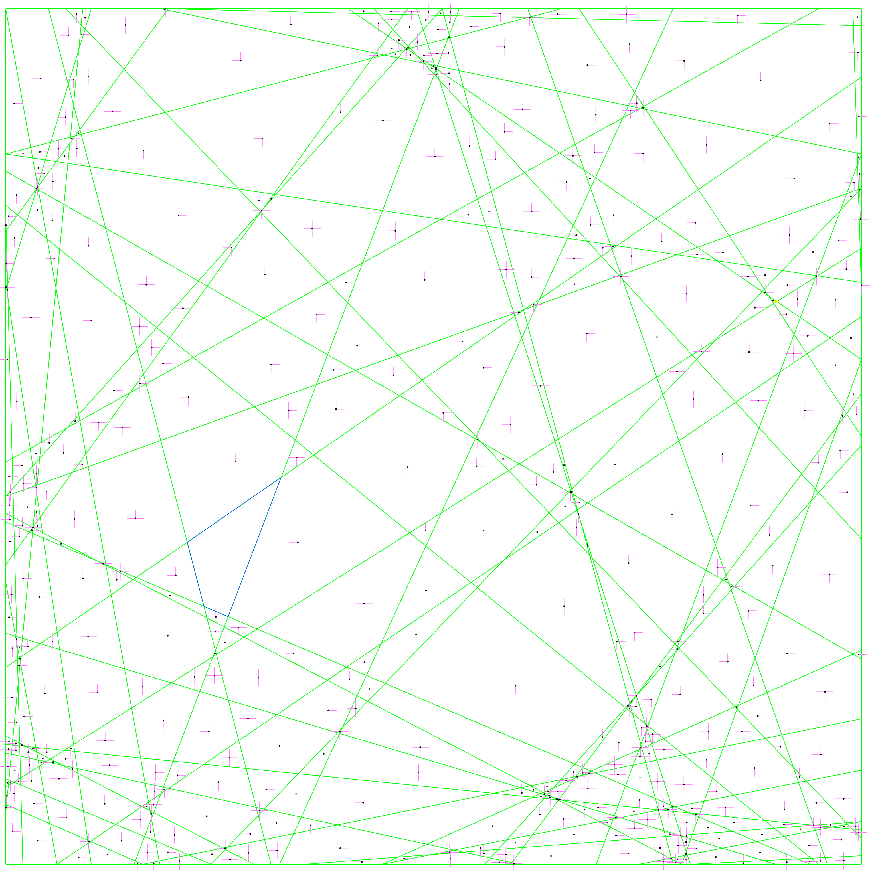
The linpreds module contains classes to generate random gridworlds with linear predicates. This is done by choosing at random linear predicates on a grid where the endpoints of the linear predicates are in . We then assign random actions to each of the regions that are created by the intersections of these linear predicates. It also includes functions to generate a PRISM program from the gridworld.
The polygons module contains the infrastructure to translate the linear predicates generated into a data structure which makes the backward winning region construction efficient. We use the half-edge data structure (popular in computational geometry) by looking at the gridworld as a planar tiling of the grid with polygons. The backward_reachability module constructs the tree of the winning region. The game.continuous module implements a reinforcement learning-like game environment which can simulate a policy for instances of LINGRID. Lastly, policy.subgoals implements Algorithm 1 and can synthesize programmatic policies from a path of segments.
The benchmarks folder contains a set of 17 benchmarks including the spiral and double-pass triangle examples. The others were generated by our code and go up to instances with 50 linear predicates and 600+ regions. The synthesized policies can be seen and the policy path visualized in images in the respective folders of the benchmarks. The benchmark data can be found in Table 1. We measure size in bytes to take into account the size of numerical coefficients involved. We observe that the size of the policy is polynomial (almost linear) in the size of the gridworld. Note that the size of the gridworld is the space required to store all the edges of all the regions of the gridworld.
| Benchmark | Gridworld size | Policy size | Regions |
|---|---|---|---|
| spiral | 10833 | 20847 | 14 |
| size3preds5loopy | 8786 | 15744 | 11 |
| size50preds10-1 | 30669 | 57926 | 32 |
| size50preds20-1 | 105252 | 126263 | 113 |
| size100preds20-1 | 119253 | 136257 | 126 |
| size100preds20-2 | 108256 | 130591 | 115 |
| size100preds30-1 | 228676 | 256031 | 233 |
| size100preds30-2 | 220557 | 248063 | 230 |
| size100preds30-3 | 221308 | 244846 | 227 |
| size100preds30-4 | 266882 | 303592 | 271 |
| size100preds50-1 | 612940 | 655357 | 616 |
| size100preds50-2 | 668670 | 706836 | 668 |
| size100preds50-3 | 635978 | 663439 | 628 |
| size100preds50-4 | 538503 | 576528 | 542 |
| size100preds50-5 | 603314 | 641681 | 616 |
9 Conclusions and future work
This work is a first step towards theoretical foundations of programmatic reinforcement learning, and more specifically the question of designing programming languages for policies. The take away message is that for a large class of environments we were able to construct programmatic policies using in a non-trivial way control loops. We proved expressiveness results, meaning existence of optimal programmatic policies, as well as succinctness results, proving that there exist optimal programmatic policies whose size are independent from the number of states (and only on the number of regions). We hope that this paper will open a fruitful line of research on the theoretical front. We outline here promising directions.
A burning question is studying the trade-offs between sizes of programmatic policies and their performances. In this paper, we focused on winning policies, meaning paths to the target region. For the case of deterministic gridworlds, the length of the path is a natural measure of performance: are there small programmatic policies ensuring optimal or near optimal number of steps? More generally, performance should be measured as the expected total reward they ensure.
The motivations of this work is to construct programmatic policies because they are readable, interpretable, and verifiable. Hence alongside with expressivity and succinctness results, we should also investigate how we can reason with programmatic policies, and in particular verify them. Developing verification algorithms for programmatic policies is a natural next step for this work. Another desirable property is generalizability: programmatic policies are expected to generalize better, as it was argued in the original papers [4, 10, 20]. Further theoretical and empirical studies will help us understand this argument better.
Last but not least, once we understand which classes of programmatic policies are expressive and succinct, remains the main question: how do we learn programmatic policies? Many approaches have been developed for decision trees, PIDs, and related classes. Learning more structured programmatic policies involving control loops is a very exciting challenge for the future, which has been tackled very recently [14, 1, 5]!
References
- [1] David S. Aleixo and Levi H. S. Lelis. Show me the way! Bilevel search for synthesizing programmatic strategies. In Conference on Artificial Intelligence, AAAI, pages 4991–4998. AAAI Press, 2023. URL: https://doi.org/10.1609/aaai.v37i4.25626, doi:10.1609/AAAI.V37I4.25626.
- [2] Roman Andriushchenko, Milan Ceska, Sebastian Junges, and Joost-Pieter Katoen. Inductive synthesis of finite-state controllers for POMDPs. In Proceedings of the Conference on Uncertainty in Artificial Intelligence, UAI, volume 180 of Proceedings of Machine Learning Research, pages 85–95. PMLR, 2022. URL: https://proceedings.mlr.press/v180/andriushchenko22a.html.
- [3] Karl Johan Åström and Tore Hägglund. PID Controllers: Theory, Design, and Tuning. ISA - The Instrumentation, Systems and Automation Society, 1995.
- [4] Osbert Bastani, Yewen Pu, and Armando Solar-Lezama. Verifiable reinforcement learning via policy extraction. In Annual Conference on Neural Information Processing Systems, NeurIPS, pages 2499–2509, 2018. URL: https://proceedings.neurips.cc/paper/2018/hash/e6d8545daa42d5ced125a4bf747b3688-Abstract.html.
- [5] Kevin Batz, Tom Jannik Biskup, Joost-Pieter Katoen, and Tobias Winkler. Programmatic strategy synthesis: Resolving nondeterminism in probabilistic programs. Proceedings of the ACM on Programming Languages, 8(POPL):2792–2820, January 2024. URL: http://dx.doi.org/10.1145/3632935, doi:10.1145/3632935.
- [6] Ahmed Bouajjani, Javier Esparza, and Oded Maler. Reachability analysis of pushdown automata: Application to model-checking. In International Conference on Concurrency Theory, CONCUR, volume 1243 of Lecture Notes in Computer Science, pages 135–150. Springer, 1997. doi:10.1007/3-540-63141-0\_10.
- [7] Arnaud Carayol and Olivier Serre. Pushdown games. In Nathanaël Fijalkow, editor, Games on Graphs. Arxiv, 2023.
- [8] Nathanaël Fijalkow, Nathalie Bertrand, Patricia Bouyer-Decitre, Romain Brenguier, Arnaud Carayol, John Fearnley, Hugo Gimbert, Florian Horn, Rasmus Ibsen-Jensen, Nicolas Markey, Benjamin Monmege, Petr Novotný, Mickael Randour, Ocan Sankur, Sylvain Schmitz, Olivier Serre, and Mateusz Skomra. Games on Graphs. Online, 2023.
- [9] Christian Hensel, Sebastian Junges, Joost-Pieter Katoen, Tim Quatmann, and Matthias Volk. The probabilistic model checker Storm. International Journal on Software Tools for Technology Transfer, 24(4):589–610, 2022. URL: https://doi.org/10.1007/s10009-021-00633-z, doi:10.1007/S10009-021-00633-Z.
- [10] Jeevana Priya Inala, Osbert Bastani, Zenna Tavares, and Armando Solar-Lezama. Synthesizing programmatic policies that inductively generalize. In International Conference on Learning Representations, ICLR. OpenReview.net, 2020. URL: https://openreview.net/forum?id=S1l8oANFDH.
- [11] Marta Z. Kwiatkowska, Gethin Norman, and David Parker. PRISM 4.0: Verification of probabilistic real-time systems. In International Conference on Computer Aided Verification, CAV, volume 6806 of Lecture Notes in Computer Science, pages 585–591. Springer, 2011. doi:10.1007/978-3-642-22110-1\_47.
- [12] Mikel Landajuela, Brenden K. Petersen, Sookyung Kim, Cláudio P. Santiago, Ruben Glatt, T. Nathan Mundhenk, Jacob F. Pettit, and Daniel M. Faissol. Discovering symbolic policies with deep reinforcement learning. In International Conference on Machine Learning, ICML, volume 139 of Proceedings of Machine Learning Research, pages 5979–5989. PMLR, 2021. URL: http://proceedings.mlr.press/v139/landajuela21a.html.
- [13] Jacky Liang, Wenlong Huang, Fei Xia, Peng Xu, Karol Hausman, Brian Ichter, Pete Florence, and Andy Zeng. Code as policies: Language model programs for embodied control. In IEEE International Conference on Robotics and Automation, ICRA, pages 9493–9500. IEEE, 2023. doi:10.1109/ICRA48891.2023.10160591.
- [14] Rubens O. Moraes, David S. Aleixo, Lucas N. Ferreira, and Levi H. S. Lelis. Choosing well your opponents: How to guide the synthesis of programmatic strategies. In International Joint Conference on Artificial Intelligence, IJCAI, pages 4847–4854. ijcai.org, 2023. URL: https://doi.org/10.24963/ijcai.2023/539, doi:10.24963/IJCAI.2023/539.
- [15] Petr Novotny. Markov decision processes. In Nathanaël Fijalkow, editor, Games on Graphs. Arxiv, 2023.
- [16] Wenjie Qiu and He Zhu. Programmatic reinforcement learning without oracles. In International Conference on Learning Representations, ICLR. OpenReview.net, 2022. URL: https://openreview.net/forum?id=6Tk2noBdvxt.
- [17] Xinghua Qu, Zhu Sun, Yew-Soon Ong, Abhishek Gupta, and Pengfei Wei. Minimalistic attacks: How little it takes to fool deep reinforcement learning policies. IEEE Transactions on Cognitive and Developmental Systems, 13(4):806–817, 2021. doi:10.1109/TCDS.2020.2974509.
- [18] David Silver, Thomas Hubert, Julian Schrittwieser, Ioannis Antonoglou, Matthew Lai, Arthur Guez, Marc Lanctot, Laurent Sifre, Dharshan Kumaran, Thore Graepel, Timothy Lillicrap, Karen Simonyan, and Demis Hassabis. A general reinforcement learning algorithm that masters chess, shogi, and go through self-play. Science, 362(6419):1140–1144, 2018. URL: https://www.science.org/doi/abs/10.1126/science.aar6404, arXiv:https://www.science.org/doi/pdf/10.1126/science.aar6404, doi:10.1126/science.aar6404.
- [19] Niko Sünderhauf, Oliver Brock, Walter J. Scheirer, Raia Hadsell, Dieter Fox, Jürgen Leitner, Ben Upcroft, Pieter Abbeel, Wolfram Burgard, Michael Milford, and Peter Corke. The limits and potentials of deep learning for robotics. International Journal on Robotics Research, 37(4-5):405–420, 2018. doi:10.1177/0278364918770733.
- [20] Dweep Trivedi, Jesse Zhang, Shao-Hua Sun, and Joseph J. Lim. Learning to synthesize programs as interpretable and generalizable policies. In Annual Conference on Neural Information Processing Systems, NeurIPS, pages 25146–25163, 2021. URL: https://proceedings.neurips.cc/paper/2021/hash/d37124c4c79f357cb02c655671a432fa-Abstract.html.
- [21] Abhinav Verma, Hoang Minh Le, Yisong Yue, and Swarat Chaudhuri. Imitation-projected programmatic reinforcement learning. In Annual Conference on Neural Information Processing Systems, NeurIPS, pages 15726–15737, 2019. URL: https://proceedings.neurips.cc/paper/2019/hash/5a44a53b7d26bb1e54c05222f186dcfb-Abstract.html.
- [22] Abhinav Verma, Vijayaraghavan Murali, Rishabh Singh, Pushmeet Kohli, and Swarat Chaudhuri. Programmatically interpretable reinforcement learning. In International Conference on Machine Learning, ICML, volume 80 of Proceedings of Machine Learning Research, pages 5052–5061. PMLR, 2018. URL: http://proceedings.mlr.press/v80/verma18a.html.
- [23] Oriol Vinyals, Igor Babuschkin, Wojciech M. Czarnecki, Michaël Mathieu, Andrew Dudzik, Junyoung Chung, David H. Choi, Richard Powell, Timo Ewalds, Petko Georgiev, Junhyuk Oh, Dan Horgan, Manuel Kroiss, Ivo Danihelka, Aja Huang, Laurent Sifre, Trevor Cai, John P. Agapiou, Max Jaderberg, Alexander Sasha Vezhnevets, Rémi Leblond, Tobias Pohlen, Valentin Dalibard, David Budden, Yury Sulsky, James Molloy, Tom Le Paine, Çaglar Gülçehre, Ziyu Wang, Tobias Pfaff, Yuhuai Wu, Roman Ring, Dani Yogatama, Dario Wünsch, Katrina McKinney, Oliver Smith, Tom Schaul, Timothy P. Lillicrap, Koray Kavukcuoglu, Demis Hassabis, Chris Apps, and David Silver. Grandmaster level in starcraft II using multi-agent reinforcement learning. Nature, 575(7782):350–354, 2019. URL: https://doi.org/10.1038/s41586-019-1724-z, doi:10.1038/S41586-019-1724-Z.
- [24] He Zhu, Zikang Xiong, Stephen Magill, and Suresh Jagannathan. An inductive synthesis framework for verifiable reinforcement learning. In ACM SIGPLAN Conference on Programming Language Design and Implementation, PLDI, pages 686–701. ACM, 2019. doi:10.1145/3314221.3314638.