Nonlinear harmonic spectra in bilayer van der Waals antiferromagnets CrX₃

Abstract

Bilayer antiferromagnets CrX₃ (X $=$ Cl, Br, and I) are promising materials for spintronics and optoelectronics that are rooted in their peculiar electronic structures. However, their bands are often hybridized from the interlayer antiferromagnetic ordering, which are difficult to disentangle by traditional methods. In this work, we theoretically show that nonlinear harmonic spectra can differentiate subtle differences in their electronic states. In contrast to prior nonlinear optical studies which often use one or two photon energies, we systematically study the wavelength-dependent nonlinear harmonic spectra realized by hundreds of individual dynamical simulations under changed photon energies. Through turning on and off some excitation channels, we can pinpoint every dipole-allowed transition that largely contributes to the second and third harmonics. With the help of momentum matrix elements, highly entangled resonance peaks at a higher energy above the band edge can be assigned to specific transitions between the valence bands and three separate regions of conduction bands. Our findings demonstrate a feasible means to detect very complex electronic structures in an important family of two-dimensional antiferromagnets.

I I. Introduction

Among two-dimensional van der Waals (vdW) magnetic materials discovered so far, bilayers CrX₃ (X = Cl, Br, and I) stand out as a key group of materials for spintronics and optoelectronics. They exhibit remarkable electronic and optical properties CrCl-data ; CrBr-data ; CrI-data1 ; CrI-data2 ; CrI-data3 that are unparalleled by other materials. The interlayer magnetic coupling between adjacent ferromagnetic monolayers of CrX₃ can be manipulated by applying external fields electric2 ; electric3 ; pressure1 ; pressure2 ; pressure3 or adjusting the stacking patterns stacking1 ; stacking2 . Different interlayer magnetic couplings in bilayers CrX₃ are vital to tunnel magnetoresistance. More notably, bilayers CrX₃ provide an excellent platform for studying light-matter interactions such as magneto-optic Kerr effect MOKE , magnetic circular dichroism RMCD , polarized photoluminescence PL , and second harmonic generation (SHG) shg1 ; shg2 . Further progress is not possible without a detailed understanding of their electronic states. Nonlinear optical techniques such as SHG, third or high harmonic generation (HHG) solid2 ; solid3 ; C60 ; reconstruct1 ; reconstruct2 ; reconstruct3 and deliver attosecond laser pulses ferray1988 , are a method of choice. Based on the three-step model proposed by Vampa et al. three-step , the valence and conduction bands during excitation are selected by the wavelength of a laser pulse. They have shown that the interband contribution is more pronounced with a shorter wavelength three-step . In ZnO, the high harmonic spectra up to the 25th order are generated by the driving laser with wavelengths of 3250 nm, where the maximum cutoff is determined by the maximum energy difference between the valence and conduction bands experiment-cutoff . Decreasing wavelength to 800 nm, Osika et al. predict that the cutoff moves to the lower harmonics theory-cutoff . This wavelength dependence is confirmed in a model system inter-intra . In monolayer MoS₂, Liu et al. report that the even- and odd-harmonics are extended to the 13th order under the wavelength of 4133 nm. It is found that the even-order harmonic intensity is much smaller than that of the odd harmonic, implying the different excited origins of these two kinds of harmonics solid3 . This conclusion is also theoretically confirmed from the decreased wavelength MoS2 . All the above studies reveal that the underlying physics of nonlinear optical response depends on the wavelength of the applied laser pulses. In fact, both experimental and theoretical studies have already pointed out that the wavelength dependence of harmonics is a key characteristics of solids, which is different from the cases in atoms and small molecules. In experiments, Sun et al. extracted SHG susceptibilities $|\chi^{(2)}_{xxx}|$ and $|\chi^{(2)}_{xyy}|$ of bilayer CrI₃ by scanning 17 excitation wavelengths in the range from 800 nm to 1040 nm shg1 . At relatively low photon energies, the intensities of the resonance peaks are weak, but as the photon energy gradually increases, their intensities are strong. However, due to a small number of photon energies used, some important resonance peaks may be missed, which is crucial for analyzing the electronic state of the material. This motivates us to carry out a systematic study.

In this work, we demonstrate that nonlinear harmonics in a group of bilayers CrX₃ can pinpoint electronic states, state by state, by scanning the photon energy between 0.3$-$1.4 eV in steps of 0.01 or 0.02 eV, rather than one or two photon energies often employed. The first peaks of the 2nd harmonic spectra, resulting from the real electronic transitions between the valence and conduction bands, are the onset of the optical band gaps for each CrX₃. As the band gap gradually decreases with halogens down the periodic table, the peaks red shift. Above the first peak, complex peaks are attributed to the resonance transitions. We verify the reliability of the 2nd harmonic spectra by the continuous wave (cw) SHG. For CrCl₃, the 2nd harmonic peaks, consisting of three eigenpeaks I, II, and III, are associated with the conduction bands between 1.6$-$2.0 eV, called region 1 or $R_{1}$. These three eigenpeaks are dominated by the transitions between the valence bands and the conduction bands in $R_{1}$. The eigenpeaks result from the dipole-allowed transitions, where the incident photon energy matches the energy difference between the valence and conduction bands, and the corresponding momentum matrix elements are also large. The same is true for the other two materials CrBr₃ and CrI₃. In the 3rd harmonic spectra, fifteen transition channels are identified from the same strategy. Our study demonstrates the potential power of nonlinear harmonic spectra by mapping out the electronic states through a systematic scan of many incident photon energies, which complements the experimental studies shg1 .

The rest of the paper is arranged as follows. In Sec. II, we show our theoretical methods. Then, the results and discussions are given in Sec. III. Section IV focuses on the third harmonic and the underlying physical picture. Finally, we conclude our work in Sec. V.

II II. Theoretical Methods

We employ the first-principles method combined with the Liouville equation to simulate the dynamical nonlinear optical response. The electronic structures for bilayers CrX₃ are calculated in the framework of density functional theory (DFT), which is implemented in WIEN2k method1 ; method2 ; method3 . We employ the generalized gradient approximation (GGA) for exchange-correlation potential in the form of Perdew-Burke-Ernzerhof (PBE) PBE . We self-consistently solve the Kohn-Sham equation KS1 ; KS2 ; KS3 as,

$$\left[-\frac{\hbar^{2}}{2m_{e}}\nabla^{2}+V_{\rm eff}({\bf r})\right]\psi_{n{\bf k}}({\bf r})=E_{n{\bf k}}\psi_{n{\bf k}}({\bf r}),$$ (1)

where $\psi_{n\bf{k}}(\bf{r})$ is the Bloch wave function of band index $n$ at crystal momentum $\bf{k}$, and $E_{n\bf{k}}$ denotes the corresponding eigenvalue. The first and second terms of the Hamiltonian are the kinetic energy and the Kohn-Sham effective potential, respectively. In our calculations, the plane wave expansion is determined by a cutoff parameter $R_{mt}K_{max}$ = 7.0. Dense $k$-sample points with $32\times 32\times 1$ are used to ensure the convergence of the total energy. All calculations are performed under the spin-orbit coupling (SOC), which are realized through the second variational method. The experimental lattice constants of 5.94, 6.30, and 6.87 Å are used for CrCl₃, CrBr₃, and CrI₃, respectively CrBr-data ; lattice1 ; lattice3 . The AB-stacking order is taken for bilayers CrX₃. The unit cell contains four Cr atoms and twelve X atoms. The interlayer distances for CrCl₃, CrBr₃, and CrI₃ are 5.76, 6.05, and 6.82 Å, respectively stacking2 . To mimic the two-dimensional geometry, a vacuum layer of height 16 Å is inserted between the bilayers along the $z$ direction.

To obtain HHG, we first construct the density matrix of the ground state as $\rho_{0}=|\psi_{n{\bf k}}({\bf r})\rangle\langle\psi_{n{\bf k}}({\bf r})|$. Then, the dynamic density matrix can be obtained by numerically solving the time-dependent Liouville equation LV1 ; LV2 ; LV3

$$i\hbar\langle m{\bf k}|\partial\rho/\partial t|n{\bf k}\rangle=\langle m{\bf k}|[{\cal H},\rho]|n{\bf k}\rangle,$$ (2)

where $\rho$ is the time-dependent density matrix, and a generic Hamiltonian is expressed as ${\cal H}={\cal H}_{0}+{\cal H}_{I}$. ${\cal H}_{0}$ is the system Hamiltonian. ${\cal H}_{I}$ is the interaction Hamiltonian between the laser field and the system: ${\cal H}_{I}=\frac{e}{m_{e}}\hat{{\bf P}}\cdot{\bf A}(t)$, where $\hat{{\bf P}}$ is the momentum operator, and ${\bf A}(t)$ represents the vector potential of the laser field. The detailed vector potential used in this work is ${\bf A}(t)=A_{0}e^{-t^{2}/\tau^{2}}[$cos$(\omega t){\bf\hat{n}}]$ with ${\bf\hat{n}}$ being the unit vector of laser pulse polarization. The vector potential amplitude is taken as $A_{0}$ = 0.03 Vfs/Å and the duration $\tau$ is set to 60 fs. The incident photon energies $\hbar\omega$ range from 0.3 to 1.4 eV at steps of 0.01 or 0.02 eV. After obtaining the time-dependent density matrix $\rho$, we can calculate the expectation value of momentum operator mumentum through ${\bf P}(t)=\Sigma_{{\bf k}}{\rm Tr}[\rho_{{\bf k}}(t)\hat{{\bf P}}_{{\bf k}}]$ with $\hat{{\bf P}}_{{\bf k}}=-i\hbar\nabla$. Finally, we get the harmonic spectra by Fourier transforming ${\bf P}(t)$ into the frequency domain by ${\bf P}(\omega)=\int_{-\infty}^{\infty}{\bf P}(t)e^{i\omega t}{\cal W}(t)dt$ with $\omega$ being the harmonic frequency and ${\cal W}(t)$ the window function.

III III. Results and discussions

III.1 A. Static properties and cw SHG

The crystal structure of bilayers CrX₃ is displayed in the bottom panel of Fig. 1(a). Bilayers CrX₃ have S₆ point group. There are six symmetry operations that can be generated by the inversion symmetry $\cal{I}$ and the threefold rotational symmetry $C_{3}$ with the trigonal axis as the $z$ axis. It should be noted that $\cal{I}$ is broken from the interlayer antiferromagnetic (AFM) ordering with the magnetization of the monolayer along the $z$ axis, denoted as AFM-$z$. Under AFM-$z$, the combined symmetry $\cal{IT}$ is preserved with $\cal{T}$ being the time reversal symmetry. The band structure of CrCl₃ is given in Fig. 1(b). All those bands are doubly degenerate, which is protected by $\mathcal{IT}$ Kramers . The valence bands near the Fermi level are mainly from the Cr-$d$ orbitals. Below them, the bands mainly come from the Cl-$p$ orbitals. Above the Fermi level, the conduction bands mainly come from the Cr-$d$ orbitals, which are grouped into three separate regions $R_{1}$$-$$R_{3}$.

The nonlinear optical response has the potential to reveal the physical properties of a material from the light-matter interaction. The resonant enhancement is crucial to detect the band structure of a material, and has the most important contribution to the susceptibilities P1 ; P2 ; P3 . Based on the three-level model as schematically shown in the inset of Fig. 1(c), the second order susceptibility of cw SHG can be obtained as

$$\chi_{ijk}^{(2)}= \frac{Ne^{3}}{2\epsilon_{0}\hbar^{2}}\sum_{lmn}\rho_{ll}^{(0)}\bigg{[}\frac{r_{ln}^{i}r_{nm}^{j}r_{ml}^{k}}{(\omega_{nl}-2\omega-i\eta)(\omega_{ml}-\omega-i\eta)}+\frac{r_{ln}^{k}r_{nm}^{i}r_{ml}^{j}}{(\omega_{mn}-2\omega-i\eta)(\omega_{nl}+\omega+i\eta)}$$ (3)

$$+ \frac{r_{ln}^{j}r_{nm}^{i}r_{ml}^{k}}{(\omega_{nm}+2\omega+i\eta)(\omega_{ml}-\omega-i\eta)}+\frac{r_{ln}^{k}r_{nm}^{j}r_{ml}^{i}}{(\omega_{ml}+2\omega+i\eta)(\omega_{nl}+\omega+i\eta)}\bigg{]}+(j\leftrightarrow k),$$

where subscripts $i$, $j$, and $k$ of $\chi_{ijk}^{(2)}$ denote the Cartesian indices, $N$ is the atomic density, $\rho_{ll}^{(0)}$ is the initial population for the state $|l\rangle$, $\omega_{nl}=\omega_{n}-\omega_{l}$ with $\hbar\omega_{n}$ being the energy of band $n$, $\hbar\omega$ is the photon energy, $r_{ln}$ is the matrix element of the position operator between electronic states $|l\rangle$ and $|n\rangle$, and $\eta$ is the damping parameter damping1 ; damping2 . The notation ($j\leftrightarrow k$) means an exchange of the two Cartesian directions. The first term in Eq. (1) can be visualized by the double-sided Feynman diagram, as shown in the inset of Fig. 1(c). The resonant enhancement can be understood from its denominator, where two terms $(\omega_{nl}-2\omega-i\eta)$ and $(\omega_{ml}-\omega-i\eta)$ are involved. When $2\hbar\omega=\hbar\omega_{nl}$ or $\hbar\omega=\hbar\omega_{ml}$, the cw SHG susceptibility has two typical peaks: one at $\hbar\omega_{ml}$ for the transition $|m\rangle$ $\rightarrow$ $|l\rangle$ and the other at half of $\hbar\omega_{nl}$ for the transition $|n\rangle$ $\rightarrow$ $|l\rangle$. Our peaks in cw SHG originate from these resonant contributions. However, for the degenerate bands, $\hbar\omega_{nl}$ and 2$\hbar\omega_{ml}$ are usually small. This will lead to a divergence when the photon energy $\hbar\omega$ approaches zero MSHG . We are aware that the low-frequency divergence in the nonlinear optical response depends on the gauges used. Although the velocity gauge can handle the low-frequency divergence, it is problematic to truncate the summation of multiple bands exciton1 ; gauge1 . On the other hand, the length gauge takes the $k$ derivative instead of position operator to account for the local effect of wavefunctions, but to numerically compute it is challenging gauge2 . Thus, our dynamical nonlinear response approach is a better way to overcome limitation, as discussed below.

III.2 B. Dynamical response

In the perturbation theory, the first-order density matrix $\rho^{(1)}$ is computed as

$$i\hbar\dot{\rho}^{(1)}=[H_{0},\rho^{(1)}]+[H_{I},\rho^{(0)}],$$ (4)

where $H_{0}$ is the unperturbed Hamiltonian and $H_{I}$ is the interaction between the laser field and the system. The second-order density matrix is given by

$$i\hbar\dot{\rho}^{(2)}=[H_{0},\rho^{(2)}]+[H_{I},\rho^{(1)}].$$ (5)

In the interaction picture, $\rho^{(2)}$ is

$$\rho^{(2)}(t)=\frac{1}{(i\hbar)^{2}}\int_{-\infty}^{t}dt_{1}\int_{-\infty}^{t_{1}}dt_{2}\big{[}H_{I}(t_{1}),[H_{I}(t_{2}),\rho_{0}]\big{]}.$$ (6)

Because the system response is in the expectation value of the momentum operator through the trace Tr$(\rho\hat{\textbf{P}})$, the second-order response depends on $\textbf{P}_{ij}$. Although we numerically solve the Liouville equation exactly, this dependence is useful for our purpose as illustrated in Fig. 1(a), where the nonlinear response is linked to the product of multiple momentum transition matrix elements. In addition, the nonlinear optical response based on the time-dependent density matrix has no limitation of the energy difference between electronic states. This leads to a relatively accurate result near the zero photon frequency. If the excitonic effects is considered, additional resonant peaks would appear in the low frequency range exciton2 ; exciton3 , which is beyond the scope of our current work. A normal practice in HHG is to choose one or two photon energies and then to Fourier transform the expectation value of momentum operator ${\bf P}(t)=\Sigma_{{\bf k}}{\rm Tr}[\rho_{{\bf k}}(t)\hat{{\bf P}}_{{\bf k}}]$ with $\hat{{\bf P}}_{{\bf k}}=-i\hbar\nabla$ to get the spectrum as ${\bf P}(\omega)=\int_{-\infty}^{\infty}{\bf P}(t)e^{i\omega t}dt$. But this has a deficiency. Because of the energy-time uncertainty relation in the Fourier transform, one cannot resolve harmonic peaks energetically down to 0.2 eV, except that one uses an extremely long pulse. Higher harmonics need many more parameters, and even within the perturbation theory their formulas become overly convoluted. This requires a different strategy.

III.3 C. Physics of even harmonics

Nonmagnetic bilayers CrX₃ remain centrosymmetric as their monolayers. If we consider the magnetic structures of Cr atoms, the inversion symmetry is broken from the interlayer antiferromagnetic order as the top layer with spin-up magnetic orders are changed to the bottom layer with same spin-up magnetic orders under the spatial inversion operator ($\vec{r}$$\rightarrow$$-\vec{r}$) and vice versa, as shown in the bottom panel of Fig. 1(a). Meanwhile, the time reversal symmetry is also broken from this antiferromagnetic order. According to the electric-dipole approximation, the even harmonics are allowed and also time nonreciprocal, usually denoted as c-type shg1 . Our calculated HH spectra did include both the odd and even harmonics and confirm this symmetry analysis, as shown in Fig. S1(c) of the Supplemental Material (SM) SM . When the interlayer magnetic order is changed to be ferromagnetic, the spatial inversion symmetry is recovered as the top layer with spin-up magnetic orders is identical to the bottom layer under $\vec{r}$$\rightarrow$$-\vec{r}$. As a result, the even harmonics disappear, as shown in Fig. S1(d) SM . Thus, these unique magnetic structures in bilayers CrX₃ can be used to study the magnetization-mediated nonlinear harmonic spectra.

III.4 D. Photon energy scan

We scan the incident photon energies $\hbar\omega$ between 0.3 and 1.4 eV in step of 0.02 eV to obtain nonlinear harmonic spectra. Figure 1(c) shows the 2nd harmonic spectra of bilayer CrCl₃. When $\hbar\omega$ is below 0.9 eV, the 2nd harmonic signals are negligible. We understand the reason behind. 2$\hbar\omega$ corresponds to the energy 1.8 eV, about 0.1 eV above the band gap of CrCl₃, so only virtual transitions occur, which explains the negligible harmonic signal. When the photon energy is above 0.9 eV, the real electron transitions touch the bands. Thus, the first peak in this 2nd harmonic spectra can be regarded as an indicator of the band gap of a material. This is also the case for CrBr₃ and CrI₃, as displayed in Figs. 1(d) and 1(e).

As the photon energy increases, additional six peaks 2$-$7 appear for CrCl₃, as shown in Fig. 1(c). Four of them, peaks 2$-$4, and 6 are comparable to the first peak. Peaks 5 and 7 have smaller amplitudes and peaks at 1.21 and 1.33 eV, respectively. It should be noted that most of these characteristic peaks also appear in cw SHG, as discussed in SM SM (see also Refs. X1 ; X2 ; X3 ; vasp1 ; vasp2 therein). For CrBr₃, the 1st peak appears at $\hbar\omega=0.79$ eV, as shown in Fig. 1(d), thus $2\hbar\omega=1.58$ eV is only 0.16 eV above the band gap of 1.42 eV for CrBr₃. Seven peaks 2$-$8 appear after peak 1. For CrI₃, more peaks appear, but have much stronger amplitudes, as shown in Fig. 1(e).

III.5 E. Understanding the complex spectra

The peaks in Figs. 1(c)$-$1(e) are very complex, but they offer an opportunity to demonstrate the power of harmonic generation. In the following, we use an even finer step of 0.01 eV to scan the photon energy from 0.3 to 1.4 eV. This requires 110 separate runs. We focus on the 2nd harmonic spectra at $\Gamma$. Figure 2(a) shows that the harmonic amplitude is small until the photon energy reaches 0.95 eV, where peaks I$-$III, called eigenpeak, appear. Peak I has a small blueshift compared with the result in Fig. 1(c), because the conduction band minimum and the valence band maximum of CrCl₃ are not at $\Gamma$. Peak II appears at 1.13 eV, and its amplitude is large, indicating an enhanced transition at this energy difference of 2.26 eV. Peak III at 1.34 eV is very small. The difference among these eigenpeak amplitudes implies the different transitions between the valence and conduction bands. As seen above, we divide the conduction bands of CrCl₃ into three regions $R_{1}$$-$$R_{3}$, so we can determine their separate effects on the harmonic amplitude. We first exclude $R_{1}$ and find that peaks I and II disappear, and peak III decreases (the red line of Fig. 2(b)). This means that peaks I$-$III are significantly affected by the transitions between the valence bands and conduction bands in $R_{1}$. Excluding only $R_{2}$ hardly changes anything (the black line of Fig. 2(b)). When only $R_{3}$ is excluded, these three peaks are also intact. Therefore, eigenpeaks I$-$III in the 2nd harmonic spectra are mainly contributed by the transitions between the valence bands and conduction bands in $R_{1}$.

All the above discussions tell us that these eigenpeaks require resonant transitions, where the incident photon energy must match the transition energy. However, this is not the entire story. Another criterion for these eigenpeaks is large momentum matrix elements between transition bands. We calculate the momentum matrix elements for those bands that are indexed in 1$-$68 for bilayer CrCl₃, as shown in Fig. 2(c). There are seven major regions with large momentum matrix elements, which are labeled as A, B, C, D, E, F, and G, respectively. We use lower case letters $a$, $b$, $c$, $d$, $e$, $f$, and $g$ for each transition in these regions, respectively. Region A contains two main transitions $a_{1}$ and $a_{2}$, as shown in Fig. 2(d). $a_{1}$ is the transition from the valence bands 35 and 36 to the conduction bands 41 and 42 in $R_{1}$, where both the valence and conduction bands are doubly degenerate. In Table I, we label it as 35,36$\rightarrow$41,42. The transition energy of $a_{1}$ is about 2.02 eV, which matches the harmonic energy of peak I in Fig. 2(a). The photon energy of peak I is about 0.95 eV. Thus, $2\hbar\omega$ gives 1.90 eV and is nearly equal to the transition energy of $a_{1}$. This means that peak I comes from the transition $a_{1}$. The transition energy of $a_{2}$ is 2.16 eV, which is close to the 2nd harmonic energy of 2.26 eV for peak II. Therefore, peak II comes from $a_{2}$. There is only one transition $b$ in region B, and its transition energy is 2.66 eV. It matches the 2nd harmonic energy of 2.68 eV for peak III, so peak III is dominated by $b$. The $|\textbf{P}|$ for $a_{1}$, $a_{2}$, and $b$ are 0.03 a.u. (see Table I). This shows that one can attribute each eigenpeak down to a specific transition, where the nonzero momentum matrix elements are essential.

IV IV. Going beyond the second order and establishing a physical picture

The above finding is also true for the 3rd harmonic spectra. From the above discussion, a physical picture is emerging. The harmonic response ${\cal R}$ is related to the momentum matrix products P2

$${\cal R}^{(n)}(t)\propto\underbrace{\textbf{P}_{ij}\textbf{P}_{jk}\dots\textbf{P}_{lf}}_{n}e^{i(E_{f}-E_{i}-n\hbar\omega)t/\hbar}\cdots,$$ (7)

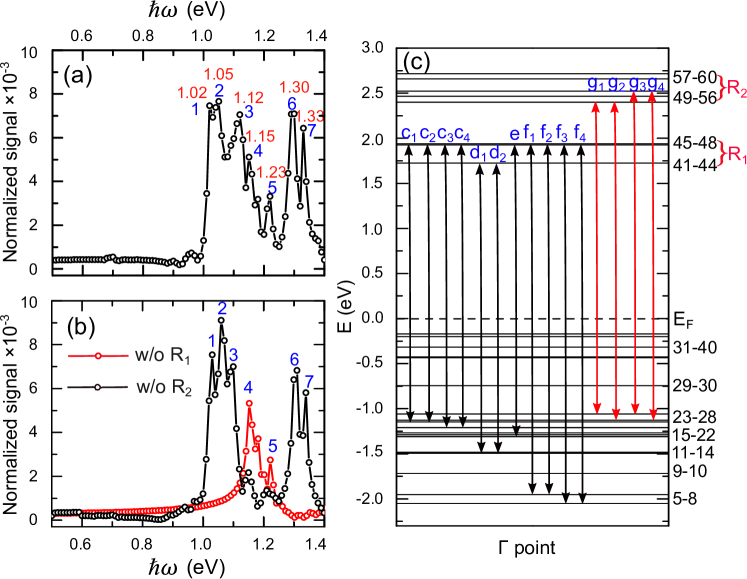
Figure 3: (a) The 3rd harmonic spectra as a function of photon energy $\hbar\omega$ at $\Gamma$. The blue and red numbers near each peak represent the peak indices and the photon energies, respectively. (b) The 3rd harmonic spectra as a function of photon energy excluding $R_{1}$ (red line) and $R_{2}$ (black line) in the conduction bands. (c) The energy diagram at $\Gamma$ for bilayer CrCl₃, where the arrows denote transitions with large P, and the letters on the arrow label different transitions.

where $n$ is the order of interaction and the time-dependent exponent highlights the most important term only. Obviously Eq. (5) is overly simplified P2 , but it captures the essential physics of the very complex processes during laser excitation as already seen in Eq. (4). This response function replaces the susceptibility $\chi^{(n)}$ in the cw limit. The finding is also true for the 3rd harmonic spectra. Figure 3(a) shows the 3rd harmonic spectra at $\Gamma$ for CrCl₃, where the photon energy is scanned from 0.5 to 1.4 eV in step of 0.01 eV. The first peak is at 1.02 eV, followed by six additional peaks 2$-$7. Peaks 1$-$3, 6, and 7 have comparable amplitudes, while peaks 4 and 5 are relatively small. Figure 3(b) presents two sets of data: one excludes $R_{1}$ and the other excludes $R_{2}$. When only $R_{1}$ is excluded (the red line), the original peaks 1, 2, and 3 disappear. Peaks 6 and 7 are largely reduced, while peaks 4 and 5 are almost unchanged. This indicates that peaks 1$-$3, 6, and 7 are dominated by the transitions between the valence bands and conduction bands in $R_{1}$. When we only exclude $R_{2}$ (the black line), peaks 1$-$3, 6, and 7 remain almost unchanged, but peaks 4 and 5 are sharply reduced. This means that those transitions are closely related to peaks 4 and 5. When we only exclude $R_{3}$, seven peaks are unchanged, indicating that these peaks are dominated by $R_{1}$ and $R_{2}$.

Recall Fig. 2(c), where we have five regions C$-$G with large momentum matrix elements $|\textbf{P}|$ between the valence bands and conduction bands in $R_{1}$ and $R_{2}$. Figure 3(c) shows the energy diagram and five regions from C to G, each of which has multiple transitions. Region C contains four transitions: $c_{1}$, $c_{2}$, $c_{3}$, and $c_{4}$, as shown in Fig. 3(c) and Table I. The transition energy of $c_{1}$ is about 3.07 eV, which matches the 3rd harmonic energy of 3.06 eV for peak 1 in Fig. 3(a). This shows that peak 1 mainly comes from the transition $c_{1}$. The transition energy of $c_{2}$ is only 0.01 eV larger than that of $c_{1}$, so it also contributes to peak 1. Comparing with $c_{1}$ and $c_{2}$, $c_{3}$ and $c_{4}$ have slightly larger transition energies of 3.14 and 3.15 eV, which generate peak 2 with $3\hbar\omega=3.15$ eV. The absolute value of $|\textbf{P}|$ for $c_{1}$ and $c_{2}$ is about 0.18 and 0.15 a.u. (see Table I). The other two transitions $c_{3}$ and $c_{4}$ have almost equal $|\textbf{P}|$ with the values of 0.13 and 0.15 a.u., respectively, which explains their comparable amplitudes of peaks 1 and 2, as shown in Fig. 3(a). Region D contains two transitions $d_{1}$ and $d_{2}$, as shown in Fig. 3(c). The corresponding transition energies are 3.20 eV and 3.21 eV, which contribute to peak 2. The transitions $d_{1}$ and $d_{2}$ have a smaller $|\textbf{P}|$ of 0.11 a.u.. Region E has only one transition $e$, and the corresponding transition energy is 3.26 eV. It matches the harmonic energy of peak 3, where $3\hbar\omega=3.36$ eV. The $|\textbf{P}|$ of this transition is 0.09 a.u., which is smaller than those of peaks 1 and 2. This leads to the amplitude of peak 3 smaller than those of peaks 1 and 2. For region F, there are four transitions $f_{1}$$-$$f_{4}$ with the transition energies of 3.88, 3.89, 3.98, and 3.99 eV, respectively. These transition energies are close to the harmonic energies of peaks 6 and 7 with $3\hbar\omega=3.90$ and 3.99 eV, indicating that these two peaks are mainly from the transitions $f_{1}$$-$$f_{4}$ (see Fig. 3(c)). The corresponding $|\textbf{P}|$ are 0.11, 0.11, 0.12, and 0.11 a.u., respectively. It is found that the $|\textbf{P}|$ of peaks 6 and 7 is almost equal, so the amplitudes of these two peaks are also close, as shown in Fig. 3(a).

As shown in Fig. 2(c), we can see that only one region G related to $R_{2}$ has large momentum matrix elements. It mainly contains four transitions $g_{1}$, $g_{2}$, $g_{3}$, and $g_{4}$, as shown in Fig. 3(c) and Table I. Their transition energies are 3.46, 3.53, 3.56, and 3.65 eV, respectively. The first three transition energies almost match the harmonic energy of peak 4 with $3\hbar\omega=3.45$ eV. This indicates that these three transitions contribute to peak 4. This is the reason why peak 4 is so broad. However, only one transition $g_{4}$ contributes to peak 5 with $3\hbar\omega=3.69$ eV, giving rise to a narrow peak in comparison with peak 4. In addition, the momentum matrix elements $|\textbf{P}|$ of $g_{1}$$-$$g_{3}$ are 0.23, 0.20, and 0.13 a.u., respectively. By contrast, $g_{4}$ has a slightly smaller $|\textbf{P}|$ of 0.11 a.u.. As a result, the amplitude of peak 5 is smaller than that of peak 4.

It is found that the amplitudes of eigenpeaks for the 3rd harmonic spectra are larger than those for the 2nd harmonic spectra. The appearance of the strong eigenpeaks needs large $|\textbf{P}|$. In fact, $|\textbf{P}|$ in regions C$-$G did have much larger values than those in regions A and B, as shown in Fig. 2(c). The underlying physics comes from the fact that $|\textbf{P}|$ contributing to the 2nd harmonic spectra are related to the valence bands 29$-$40 and the conduction bands in $R_{1}$, which are mainly dominated by the same Cr-$d$ orbitals, as shown in Fig. 1(b). However, $|\textbf{P}|$ for the 3rd harmonic spectra involves a larger energy difference. The corresponding valence bands are much lower, which are mainly from the Cl-$p$ orbitals and are denoted as the bands 1$-$28 in Fig. 1(b). Compared to $|\textbf{P}|$ related to the 2nd harmonic spectra, $|\textbf{P}|$ for the 3rd harmonic spectra would be much larger as the transitions belong to different orbitals. Our calculated momentum matrix elements confirm this conclusion (see Table I for more details).

V V. Conclusions

We have demonstrated that the nonlinear harmonic spectra in a group of bilayers CrX₃ can pinpoint specific transitions between valence and conduction bands. We scan over 100 photon energies from 0.3$-$1.4 eV in fine steps. We map out the momentum transition matrix elements and calculate the corresponding contributions to the harmonic spectra. By including and excluding some transitions, we can directly correlate each peak in both the 2nd and 3rd harmonic spectra to a specific transition, which has not been possible previously because often time only one or two photon energies are used. The first resonance peak in the 2nd harmonic spectra serves as the onset of the band gap of a material. Complex peaks can now be attributed to the intrinsic electronic properties. All the results are further confirmed by the 3rd harmonic spectra. Our findings unleash the power of nonlinear harmonic spectra to study the vdW antiferromagnets, and are likely to motivate future experimental studies beyond CrI₃ shg1 .

Table 1: Transitions in regions A$-$G in Fig. 2(c), with large momentum matrix elements $|\textbf{P}|$. The corresponding transition energies match the harmonic energies of the eigenpeaks, where I$-$III denote the peaks in the 2nd harmonic spectra and 1$-$7 denote those eigenpeaks in the 3rd harmonic spectra. $\Delta$$E$ and $\hbar\omega$ represent the transition and photon energies, respectively, in units of eV. The momentum matrix elements are in units of atomic unit (a.u.).

Region		Transition		$|\textbf{P}|$		$\Delta$$E$		Peak		$\hbar\omega$ (2$\hbar\omega$/3$\hbar\omega$)
A		35,36$\rightarrow$41,42		0.03		2.02 ($a_{1}$)		I		0.95 (1.90)
		31,32$\rightarrow$43,44		0.03		2.16 ($a_{2}$)		II		1.13 (2.26)
B		29,30$\rightarrow$47,48		0.03		2.66 ($b$)		III		1.34 (2.68)
C		23,24$\rightarrow$45,46		0.18		3.07 ($c_{1}$)		1		1.02 (3.06)
		23,24$\rightarrow$47,48		0.15		3.08 ($c_{2}$)		1
		21,22$\rightarrow$45,46		0.13		3.14 ($c_{3}$)		2		1.05 (3.15)
		21,22$\rightarrow$47,48		0.15		3.15 ($c_{4}$)		2
D		11,12$\rightarrow$41,42		0.11		3.20 ($d_{1}$)		2		1.05 (3.15)
		13,14$\rightarrow$43,44		0.11		3.21 ($d_{2}$)		2
E		15,16$\rightarrow$48,47		0.09		3.26 ($e$)		3		1.12 (3.36)
F		7,8$\rightarrow$45,46		0.11		3.88 ($f_{1}$)		6		1.30 (3.90)
		7,8$\rightarrow$47,48		0.11		3.89 ($f_{2}$)		6
		5,6$\rightarrow$45,46		0.12		3.98 ($f_{3}$)		7		1.33 (3.99)
		5,6$\rightarrow$47,48		0.11		3.99 ($f_{4}$)		7
G		27,28$\rightarrow$51,52		0.23		3.46 ($g_{1}$)		4		1.15 (3.45)
		25,26$\rightarrow$49,50		0.20		3.53 ($g_{2}$)		4
		27,28$\rightarrow$55,56		0.13		3.56 ($g_{3}$)		4
		25,26$\rightarrow$55,56		0.11		3.65 ($g_{4}$)		5		1.23 (3.69)

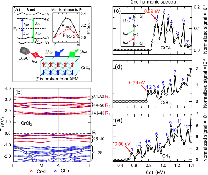
Figure 1: (a) A schematic diagram of nonlinear optical responses in bilayer CrX₃, which are related to the band structure and the momentum matrix elements P. $|\textbf{P}|$_40,42 between the bands 40 and 42 is larger than $|\textbf{P}|$_30,42 along $\Gamma$$-$$M$ in bilayer CrCl₃. (b) Orbital-resolved band structure for bilayer CrCl₃, where the red and blue circles represent the Cr-$d$ and Cl-$p$ orbitals, respectively. The band indices 1$-$68 are marked on the right side of this figure. The conduction bands are divided into three individual regions $R_{1}$$-$$R_{3}$. (c) The 2nd harmonic spectra as a function of photon energy for bilayer CrCl₃. The blue numbers near the peaks represent the peak indices and the red number is the photon energy of the first peak. The inset shows the conventional double-sided Feynman diagram corresponding to the first term in Eq. (1). The Feynman diagram has two lines of propagation, one for the $|l\rangle$ side of $\rho^{(0)}_{ll}$ and the other for the $\langle l|$ side. The red, green, and blue arrows correspond to the input photon energies $\hbar\omega$ and $\hbar\omega$ and the output photon energies $2\hbar\omega$, respectively. The energy conservation relation $\hbar\omega$ + $\hbar\omega$ = $2\hbar\omega$ is satisfied. (d) and (e) The 2nd harmonic spectra as a function of photon energy for bilayers CrBr₃ and CrI₃, respectively.

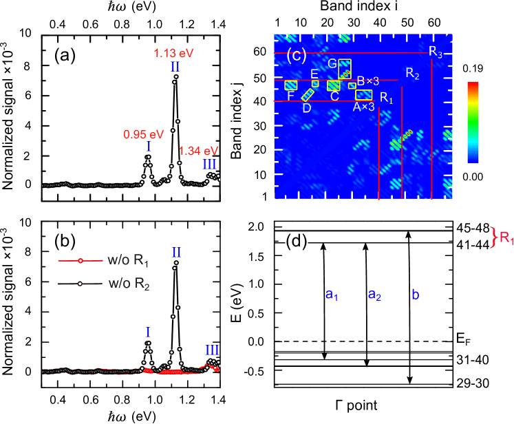
Figure 2: (a) The 2nd harmonic spectra as a function of photon energy at $\Gamma$ for bilayer CrCl₃. The blue and red numbers near each peak represent the peak indices and the corresponding photon energies, respectively. (b) The 2nd harmonic spectra as a function of photon energy excluding $R_{1}$ (red line) and $R_{2}$ (black line) in the conduction bands. (c) The absolute value of the momentum matrix elements $|\textbf{P}|$ for bands 1$-$68 in bilayer CrCl₃. (d) The energy diagram at $\Gamma$ for bilayer CrCl₃, where the arrows denote transitions with large P, and the letters on the arrow label the different transitions.

References

- (1) Z. Wang, M. Gibertini, D. Dumcenco, T. Taniguchi, K. Watanabe, E. Giannini, and A. F. Morpurgo, Nat. Nanotechnol. 14, 1116 (2019).
- (2) W. J. Chen, Z. Y. Sun, Z. J. Wang, L. H. Gu, X. D. Xu, S. W. Wu, and C. L. Gao, Science 366, 983 (2019).
- (3) T. C. Song, X. H. Cai, M. W. Tu, X. O. Zhang, B. Huang, N. P. Wilson, K. L. Seyler, L. Zhu, T. Taniguchi, K. Watanabe, M. A. McGuire, D. H. Cobden, D. Xiao, W. Yao, and X. D. Xu, Science 360, 1214 (2018).
- (4) D. R. Klein, D. MacNeill, J. L. Lado, D. Soriano, E. Navarro-Moratalla, K. Watanabe, T. Taniguchi, S. Manni, P. Canfield, J. Fernández-Rossier, and P. Jarillo-Herrero, Science 360, 1218 (2018).
- (5) Z. Wang, I. Gutiérrez-Lezama, N. Ubrig, M. Kroner, M. Gibertini, T. Taniguchi, K. Watanabe, A. Imamoǧlu, E. Giannini, and A. F. Morpurgo, Nat. Commun. 9, 2516 (2018).
- (6) B. Huang, G. Clark, D. R. Klein, D. MacNeill, E. NavarroMoratalla, K. L. Seyler, N. Wilson, M. A. McGuire, D. H. Cobden, D. Xiao, W. Yao, P. Jarillo-Herrero, and X. Xu, Nat. Nanotechnol. 13, 544 (2018).
- (7) S. Jiang, J. Shan, and K. F. Mak, Nat. Mater. 17, 406 (2018).
- (8) T. Li, S. Jiang, N. Sivadas, Z. Wang, Y. Xu, D. Weber, J. E. Goldberger, K. Watanabe, T. Taniguchi, C. J. Fennie, K. Fai Mak, and J. Shan, Nat. Mater. 18, 1303 (2019).
- (9) T. Song, Z. Fei, M. Yankowitz, Z. Lin, Q. Jiang, K. Hwangbo, Q. Zhang, B. Sun, T. Taniguchi, K. Watanabe, M. A. McGuire, D. Graf, T. Cao, J. H. Chu, D. H. Cobden, C. R. Dean, D. Xiao, and X. Xu, Nat. Mater. 18, 1298 (2019).
- (10) S. Mondal, M. Kannan, M. Das, L. Govindaraj, R. Singha, B. Satpati, S. Arumugam, and P. Mandal, Phys. Rev. B 99, 180407(R) (2019).
- (11) N. Sivadas, S. Okamoto, X. Xu, C. J. Fennie, and D. Xiao, Nano Lett. 18, 7658 (2018).
- (12) P. H. Jiang, C. Wang, D. C. Chen, Z. C. Zhong, Z. Yuan, Z. Y. Lu, and W. Ji, Phys. Rev. B 99, 144401 (2019).
- (13) B. Huang, G. Clark, E. Navarro-Moratalla, D. R. Klein, R. Cheng, K. L. Seyler, D. Zhong, E. Schmidgall, M. A. McGuire, D. H. Cobden, W. Yao, D. Xiao, P. Jarillo-Herrero, and X. D. Xu, Nature (London) 546, 270 (2017).
- (14) S. W. Jiang, L. Z. Li, Z. F. Wang, J. Shan, and K. F. Mak, Nat. Electron. 2, 159 (2019).
- (15) K. L. Seyler, D. Zhong, D. R. Klein, S. Y. Gao, X. O. Zhang, B. Huang, E. Navarro-Moratalla, L. Yang, D. H. Cobden, M. A. McGuire, W. Yao, D. Xiao, P. Jarillo-Herrero, and X. D. Xu, Nat. Phys. 14, 277 (2018).
- (16) Z. Y. Sun, Y. F. Yi, T. C. Song, G. Clark, B. Huang, Y. W. Shan, S. Wu, D. Huang, C. L. Gao, Z. H. Chen, M. McGuire, T. Cao, D. Xiao, W. T. Liu, W. Yao, X. D. Xu, and S. W. Wu, Nature 572, 497 (2019).
- (17) W. S. Song, R. X. Fei, L. H. Zhu, and L. Yang, Phys. Rev. B 102, 045411 (2020).
- (18) G. Ndabashimiye, S. Ghimire, M. Wu, D. A. Browne, K. J. Schafer, M. B. Gaarde, and D. A. Reis, Nature (London) 534, 520 (2016).
- (19) H. Z. Liu, Y. L. Li, Y. S. You, S. Ghimire, T. F. Heinz, and D. A. Reis, Nat. Phys. 13, 262 (2017).
- (20) G. P. Zhang, Phys. Rev. Lett. 95, 047401 (2005).
- (21) G. P. Zhang, M. S. Si, M. Murakami, Y. H. Bai, and T. F. George, Nat. Commun. 9, 3031 (2018).
- (22) G. P. Zhang and Y. H. Bai, Phys. Rev. B 101, 081412 (2020).
- (23) G. P. Zhang and Y. H. Bai, Phys. Rev. B 103, L100407 (2021).
- (24) M. Ferray, A. L’Huillier, X. F. Li, L. A. Lompre, G. Mainfray, and C. Manus, J. Phys. B: At. Mol. Opt. Phys. 21, L31 (1988).
- (25) G. Vampa, C. R. McDonald, G. Orlando, D. D. Klug, P. B. Corkum, and T. Brabec, Phys. Rev. Lett. 113, 073901 (2014).
- (26) S. Ghimire, A. D. DiChiara, E. Sistrunk, P. Agostini, L. F. DiMauro, and D. A. Reis, Nat. Phys. 7, 138 (2011).
- (27) E. N. Osika, A. Chacón, L. Ortmann, N. Suárez, J. A. Pérez-Hernández, B. Szafran, M. F. Ciappina, F. Sols, A. S. Landsman, and M. Lewenstein, Phys. Rev. X 7, 021017 (2017).
- (28) X. Liu, X. Zhu, X. Zhang, D. Wang, P. Lan, and P. Lu, Opt. Express 25, 29216 (2017).
- (29) M. X. Guan, C. Lian, S. Q. Hu, H. Liu, S. J. Zhang, J. Zhang, and S. Meng, Phys. Rev. B 99, 184306 (2019).
- (30) L. Jia, Z. Y. Zhang, D. Z. Yang, Y. Q. Liu, M. S. Si, G. P. Zhang, and Y. S. Liu, Phys. Rev. B 101, 144304 (2020).
- (31) L. Jia, Z. Y. Zhang, D. Z. Yang, M. S. Si, and G. P. Zhang, Phys. Rev. B 102, 174314 (2020).
- (32) L. Jia, Y. K. Song, J. L. Yao, M. S. Si, and G. P. Zhang, Phys. Rev. B 105, 214309 (2022).
- (33) J. P. Perdew, K. Burke, and M. Ernzerhof, Phys. Rev. Lett. 77, 3865 (1996).
- (34) P. Hohenberg and W. Kohn, Phys. Rev. 136, B864 (1964).
- (35) G. P. Zhang, Y. H. Bai, and T. F. George, Phys. Rev. B 80, 214415 (2009).
- (36) P. Blaha, K. Schwarz, F. Tran, R. Laskowski, G. K. H. Madsen, and L. D. Marks, J. Chem. Phys. 152, 074101 (2020).
- (37) B. Morosin and A. Narath, J. Chem. Phys. 40, 1958 (1964).
- (38) M. A. McGuire, H. Dixit, V. R. Cooper, B. C. Sales, Chem. Mater. 27, 612 (2015).
- (39) G. P. Zhang, W. Hübner, G. Lefkidis, Y. H. Bai, and T. F. George, Nat. Phys. 5, 499 (2009).
- (40) K. Blum, Density Matrix, Theory and Applications (PlenumPress, New York, 1981).
- (41) W. Schafer and M. Wegner, Semiconductor Optics and Transport Phenomena (Springer-Verlag, Berlin, 2002).
- (42) M. Murakami and G. P Zhang, Phys. Rev. A. 95, 053419 (2017).
- (43) M. J. Klein, Am. J. Phys. 20, 65 (1952).
- (44) Y. R. Shen, The Principles of Nonlinear Optics (Wiley, New York, 1984).
- (45) P. N. Butcher and D. Cotter, The Elements of Nonlinear Optics (Cambridge University Press, Cambridge, 1990).
- (46) R. W. Boyd, Nonlinear Optics (Elsevier Science, Amsterdam, 2003).
- (47) W. S. Song, G. Y. Guo, S. Huang, L. Yang, and L. Yang, Phys. Rev. Appl. 13, 014052 (2020).
- (48) Y. Q. Liu, M. S. Si, and G. P. Zhang, Phys. Rev. A 108, 033514 (2023).
- (49) V. K. Gudelli and G.-Y. Guo, Chin. J. Phys. 68, 896 (2020).
- (50) D. E. Aspnes, Phys. Rev. B 6, 4648 (1972).
- (51) Q. Ma, A. G. Grushin, and K. S. Burch, Nat. Mater. 20, 1601 (2021).
- (52) G. B. Ventura, D. J. Passos, and J. M. B. Lopes dos Santos, Phys. Rev. B 96, 035431 (2017).
- (53) R. Leitsmann, W. G. Schmidt, P. H. Hahn, and F. Bechstedt, Phys. Rev. B 71, 195209 (2005).
- (54) S. Acharya, D. Pashov, A. N. Rudenko, M. Rösner, M. v. Schilfgaarde, and M. I. Katsnelson, npj 2D Mater. Appl. 6, 33 (2022).
- (55) See Supplemental Material for more details on the theoretical methods, the electronic structures and HHG for bilayers CrX3. We also demonstrate the results of cw SHG and the 3rd harmonic spectra for CrX3. In addition, the underlying physics of eigenpeaks for the nonlinear harmonic spectra of CrBr3 and CrI3 is discussed. The Supplemental Material also contains Refs. X1 ; X2 ; X3 ; vasp1 ; vasp2 .
- (56) J. E. Sipe and E. Ghahramani, Phys. Rev. B 48, 11705 (1993).
- (57) C. Aversa and J. E. Sipe, Phys. Rev. B 52, 14636 (1995).
- (58) J. L. P. Hughes and J. E. Sipe, Phys. Rev. B 53, 10751 (1996).
- (59) G. Kresse and J. Furthmüller, Phys. Rev. B 54, 11169 (1996).
- (60) G. Kresse and D. Joubert, Phys. Rev. B 59, 1758 (1999).