Informative and non-informative decomposition of turbulent flow fields

Abstract

Not all the information in a turbulent field is relevant for understanding particular regions or variables in the flow. Here, we present a method for decomposing a source field into its informative $\bm{\Phi}_{I}(\bm{x},t)$ and residual $\bm{\Phi}_{R}(\bm{x},t)$ components relative to another target field. The method is referred to as informative and non-informative decomposition (IND). All the necessary information for physical understanding, reduced-order modelling, and control of the target variable is contained in $\bm{\Phi}_{I}(\bm{x},t)$, whereas $\bm{\Phi}_{R}(\bm{x},t)$ offers no substantial utility in these contexts. The decomposition is formulated as an optimisation problem that seeks to maximise the time-lagged mutual information of the source variable with the target variable while minimising the mutual information of its residual component. The method is applied to extract the informative and residual components of the velocity field in a turbulent channel flow, using the wall-shear stress as the target variable. We demonstrate the utility of IND in three scenarios: (i) physical insight of the effect of the velocity fluctuations on the wall-shear stress, (ii) prediction of the wall-shear stress using velocities far from the wall, and (iii) development of control strategies for drag reduction in opposition control. In case (i), IND reveals that the informative velocity related to wall-shear stress consists of wall-attached high- and low-velocity streaks, collocated with regions of vertical motions and weak spanwise velocity. This informative structure is embedded within a larger-scale streak-roll structure of residual velocity, which bears no information about the wall-shear stress. In case (ii), the best-performing model for predicting wall shear stress is a convolutional neural network that uses the informative component of the velocity as input, while the residual velocity component provides no predictive capabilities. Finally, in case (iii), we demonstrate that opposition control based on the informative wall-normal velocity yields improvements in drag reduction compared to the control based on the total or residual velocity.

1 Introduction

Since the early days of turbulence research, there have been multiple attempts to decompose the flow into different components to facilitate its physical understanding, control its behaviour and devise reduced-order models. One of the earliest examples is the Reynolds decomposition (Reynolds,, 1895), which divides the velocity field into its mean and fluctuating components. More sophisticated approaches rapidly emerged aiming at extracting the coherent structure of the flow through correlations and structure identification (Robinson,, 1991; Panton,, 2001; Adrian,, 2007; Smits et al.,, 2011; McKeon,, 2017; Jiménez,, 2018). This interest is justified by the hope that insights into the dynamics can be gained by analysing a subset of the whole flow, while the remaining incoherent flow is inconsequential. In this work, we introduce a method to decompose turbulent flow fields into informative and non-informative components, referred to as IND, such that the informative component contains all the useful information for physical understanding, modelling, and control with respect to a given quantity of interest.

The quest to divide turbulent flows in terms of coherent and incoherent motions has a long history, tracing back to the work of Theodorsen, (1952), and has been a subject of active research since the pioneering experimental visualisations of Kline et al., (1967) and the identification of large-scale coherent regions in mixing layers by Brown and Roshko, (1974). Despite this rich history, the field still lacks consensus about the definition of a coherent structure due to the variety of interpretations proposed by different researchers. One of the initial approaches to distinguish turbulent regions was the turbulent/nonturbulent discriminator circuits introduced by Corrsin and Kistler, (1954). Since then, single- and two-point correlations have become conventional tools for identifying coherent regions within the flow (e.g., Sillero et al.,, 2014). The development of more sophisticated correlation techniques, such as the linear stochastic estimation (Adrian and Moin,, 1988) and the characteristic-eddy approach (Moin and Moser,, 1989), has further improved our understanding of the coherent structure of turbulence. An alternative set of methods focuses on decomposing the flow into localised regions where certain quantities of interest are particularly intense. The first attempts, dating back to the 1970s, include the variable-interval time average method (Blackwelder and Kaplan,, 1976) for obtaining temporal structures of bursting events and its modified version, the variable-interval space average method (Kim,, 1985), for characterising spatial rather than temporal structures. With the advent of larger databases and computational resources, more refined techniques have emerged to extract three-dimensional, spatially localised flow structures. These include investigations into regions of rotating fluid (e.g., vortices Moisy and Jiménez,, 2004; Del Álamo et al.,, 2006), motions carrying most of the kinetic energy (e.g., regions of high and low velocity streaks by Hwang and Sung,, 2018; Bae and Lee,, 2021), and those responsible for most of the momentum transfer in wall turbulence (e.g., quadrant events and uniform momentum zones by Meinhart and Adrian,, 1995; Adrian et al.,, 2000; Lozano-Durán et al.,, 2012; Lozano-Durán and Jiménez,, 2014; Wallace,, 2016; de Silva et al.,, 2016).

The methods described above offer a local-in-space characterisation of coherent structures, in contrast to the global-in-space modal decompositions of turbulent flows (Taira et al.,, 2017, 2020). One of the first established global-in-space methods is the proper orthogonal decomposition (POD) (Lumley,, 1967), wherein the flow is decomposed into a series of eigenmodes that optimally reconstruct the energy of the field. This method has evolved in different directions, such as space-only POD (Sirovich,, 1987), spectral POD (Towne et al.,, 2018), and conditional POD (Schmidt and Schmid,, 2019), to name a few. Another popular approach is dynamic mode decomposition (DMD) (Schmid,, 2010; Schmid et al.,, 2011), along with decompositions based on the spectral analysis of the Koopman operator (Rowley et al.,, 2009; Mezić,, 2013). Similar to POD, various modifications of DMD have been developed, e.g., the extended DMD (Williams et al.,, 2015), the multi-resolution DMD (Kutz et al.,, 2016), and the high-order DMD (Le Clainche and Vega,, 2017) [see (Schmid,, 2022) for a review]. Another noteworthy modal decomposition approach is empirical mode decomposition, first proposed by Huang et al., (1998) and recently used in the field of fluid mechanics (e.g., Cheng et al.,, 2019). While the methods above are purely data-driven, other modal decompositions, such as resolvent analysis and input-output analysis, are grounded in the linearised Navier-Stokes equations (Trefethen et al.,, 1993; Jovanović and Bamieh,, 2005; McKeon and Sharma,, 2010). It has been shown that POD, DMD, and resolvent analysis are equivalent under certain conditions (Towne et al.,, 2018). Recently, machine learning has opened new opportunities for nonlinear modal decompositions of turbulent flows (Brunton et al.,, 2020).

The flow decomposition approaches presented above, either local or global in space, have greatly contributed to advancing our knowledge about the coherent structure of turbulence. Nonetheless, there are still open questions, especially regarding the dynamics of turbulence, that cannot be easily answered by current methodologies. Part of these limitations stem from the linearity of most methods, yet turbulence is a nonlinear system. A more salient issue perhaps lies in the fact that current methods tend to focus on decomposing source variables without accounting for other target variables of interest. In general, it is expected that different target variables would require different decomposition approaches of the source variable. For example, we might be interested in a decomposition of the velocity that is useful for understanding the wall-shear stress. Hence, the viewpoint adopted here aims at answering the question: What part of the flow is relevant to understanding the dynamics of another variable? In this context, coherent structures are defined as those containing the useful information needed to understand the evolution of a target variable.

The concept of information alluded above refers to the Shannon information (Shannon,, 1948; Cover and Thomas,, 2006), i.e., the average unpredictability in a random variable. The systematic use of information-theoretic tools for causality, modelling, and control in fluid mechanics has been recently discussed by Lozano-Durán and Arranz, (2022). Betchov, (1964) was one of the first authors to propose an information-theoretic metric to quantify the complexity of turbulence. Some works have leveraged Shannon information to analyse different aspects of two-dimensional turbulence and energy cascade models (Cerbus and Goldburg,, 2013; Materassi et al.,, 2014; Granero-Belinchon,, 2018; Shavit and Falkovich,, 2020; Lee,, 2021; Tanogami and Araki,, 2024). Information theory has also been used for causal inference in turbulent flows (Liang and Lozano-Durán,, 2016; Lozano-Durán et al.,, 2019; Wang et al.,, 2021; Lozano-Durán and Arranz,, 2022; Martínez-Sánchez et al.,, 2023), and reduced-order modelling (Lozano-Durán et al.,, 2019). The reader is referred to Lozano-Durán and Arranz, (2022) for a more detailed account of the applications of information-theoretic tools in fluid mechanics.

This work is organised as follows: The formulation of the flow decomposition into informative and non-informative components is introduced in Section 2. Section 3 demonstrates the application of the method to the decomposition of the velocity field, using wall-shear stress in a turbulent channel flow as the target variable. This decomposition is leveraged for physical understanding, prediction of the wall-shear stress using velocities away from the wall via convolutional neural networks, and drag reduction through opposition control. Finally, conclusions are presented in Section 4.

2 Methodology

2.1 IND of the source variable

Let us denote the source variable by $\bm{\Phi}(\bm{x},t)$ with $\bm{x}\in\Omega_{\bm{\Phi}}$ and the target variable by $\bm{\Psi}(\bm{x},t)$ with $\bm{x}\in\Omega_{\bm{\Psi}}$ where $\bm{x}$ and $t$ represent the spatial and time coordinates, respectively. For example, in the case of a turbulent channel flow, the source variable could be the velocity fluctuations defined over the entire domain, $\bm{\Phi}(\bm{x},t)=\bm{u}(\bm{x},t)$, and the target variable could be the shear stress vector at every point over one of the walls, $\bm{\Psi}(\bm{x},t)=\bm{\tau}_{w}(\bm{x},t)$, as shown in figure 1. We seek to decompose $\bm{\Phi}(\bm{x},t)$ into two contributions: an informative contribution to the target variable in the future, $\bm{\Psi}_{+}=\bm{\Psi}(\bm{x},t+\Delta T)$ with $\Delta T\geq 0$, and a residual term that conveys no information about $\bm{\Psi}_{+}$ (i.e., the non-informative component):

$$\bm{\Phi}(\bm{x},t)=\bm{\Phi}_{I}(\bm{x},t)+\bm{\Phi}_{R}(\bm{x},t),$$ (1)

where $\bm{\Phi}_{I}$ and $\bm{\Phi}_{R}$ are the informative and residual contributions, respectively. The decomposition is referred to as Informative/Non-informative Decomposition or IND.

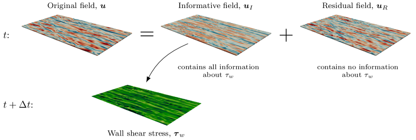
Figure 1: Schematic of IND applied to wall-bounded turbulent flow. The source variable is the velocity fluctuations in the fluid volume $\bm{x}\in\Omega_{\bm{u}}$ at $t$, and the target variable is the wall shear stress vector at the wall at $t+\Delta$. For the sake of visualisation, only the streamwise component of the velocity fluctuations and the wall shear stress is displayed. The velocity fluctuations at time $t$ are decomposed into their informative and residual components to the wall shear stress in the future, $t+\Delta t$.

To find a decomposition of the form shown in Eq. (1), we need to introduce a definition of information. We rely on the concept of Shannon information (Shannon,, 1948), which quantifies the average information in the variable $\bm{\Psi}_{+}$ as

$$H(\bm{\Psi}_{+})=-\sum_{\bm{S}\in\mathcal{S}}p_{\bm{\Psi}_{+}}(\bm{\Psi}_{+}=\bm{S})\log p_{\bm{\Psi}_{+}}(\bm{\Psi}_{+}=\bm{S})\geq 0,$$ (2)

where $H(\bm{\Psi}_{+})$ is referred to as the Shannon entropy or information of $\bm{\Psi}_{+}$, $p_{\bm{\Psi}_{+}}(\bm{\Psi}_{+}=\bm{S})$ denotes the probability of $\bm{\Psi}_{+}$ being in the state $\bm{S}$, and $\mathcal{S}$ represents the set of all possible states of $\bm{\Psi}_{+}$. The remaining information in $\bm{\Psi}_{+}$, after discounting for the information in $\bm{\Phi}$, is measured by the conditional Shannon information:

$$H(\bm{\Psi}_{+}|\bm{\Phi})=-\sum_{\bm{S}\in\mathcal{S}}\sum_{\bm{R}\in\mathcal{R}}p_{\bm{\Psi}_{+},\bm{\Phi}}(\bm{S},\bm{R})\log\frac{p_{\bm{\Psi}_{+},\bm{\Phi}}(\bm{S},\bm{R})}{p_{\bm{\Phi}}(\bm{R})}\geq 0,$$ (3)

where $p_{\bm{\Psi}_{+},\bm{\Phi}}$ is the joint probability distribution of $\bm{\Psi}_{+}$ and $\bm{\Phi}$, $\bm{R}$ is a particular state of $\bm{\Phi}$, and $\mathcal{R}$ is the set of all possible states of $\bm{\Phi}$. The difference between Eq. (2) and Eq. (3) quantifies the amount of shared information between the variables

$$I(\bm{\Psi}_{+};\bm{\Phi})=H(\bm{\Psi}_{+})-H(\bm{\Psi}_{+}|\bm{\Phi}),$$ (4)

and is referred to as the mutual information between $\bm{\Psi}_{+}$ and $\bm{\Phi}$. The condition $H(\bm{\Psi}_{+})\geq H(\bm{\Psi}_{+}|\bm{\Phi})$ –known as information can’t hurt (Cover and Thomas,, 2006)– guarantees that the $I(\bm{\Psi}_{+};\bm{\Phi})$ is always non-negative. The mutual information is equal to 0 only when the variables are independent, i.e., $p_{\bm{\Psi}_{+},\bm{\Phi}}(\bm{S},\bm{R})=p_{\bm{\Psi}_{+}}(\bm{S})p_{\bm{\Phi}}(\bm{R})$ for all possible states $\bm{S}\in\mathcal{S}$ and $\bm{R}\in\mathcal{R}$.

We are now in a position to define the conditions that $\bm{\Phi}_{I}$ and $\bm{\Phi}_{R}$ must satisfy. First, for the residual term, $\bm{\Phi}_{R}$, not to have any information about $\bm{\Psi}_{+}$, we need

$$I(\bm{\Psi}_{+};\bm{\Phi}_{R})=0.$$ (5)

Secondly, the informative contribution should maximise $I(\bm{\Psi}_{+};\bm{\Phi}_{I})$ from Eq. (4), which is achieved when

$$H(\bm{\Psi}_{+}|\bm{\Phi}_{I})=0.$$ (6)

The condition $H(\bm{\Psi}_{+}|\bm{\Phi}_{I})=0$ is mathematically equivalent to expressing $\bm{\Psi}_{+}$ as a function of $\bm{\Phi}_{I}$, namely, $\bm{\Psi}_{+}=\bm{\mathcal{F}}(\bm{\Phi}_{I})$. Since the Shannon information is based on the joint probability distribution of the variables, rather than their specific values, there are infinitely many functions that satisfy Eqs. (5) and (6). To identify a unique solution, we impose the condition that the informative contribution $\bm{\Phi}_{I}$ must reconstruct as much of the energy of the source variable $\bm{\Phi}$ as possible. With that, the final optimisation problem for IND is posed as

$$\arg\min_{\bm{\Phi}_{I}}\quad\|\bm{\Phi}-\bm{\Phi}_{I}\|^{2}\quad\mathrm{s.t.}\quad H(\bm{\Psi}_{+}|\bm{\Phi}_{I})=0,\quad I(\bm{\Phi}_{R};\bm{\Phi}_{I})=0,$$ (7)

where we have replaced $I(\bm{\Phi}_{R};\bm{\Psi}_{+})=0$ by the more restrictive condition $I(\bm{\Phi}_{R};\bm{\Phi}_{I})=0$ (Cover and Thomas,, 2006) to satisfy the property:

$$\|\bm{\Phi}\|^{2}=\|\bm{\Phi}_{I}\|^{2}+\|\bm{\Phi}_{R}\|^{2}.$$ (8)

If $\bm{\Phi}$ contains no information about $\bm{\Psi}_{+}$, then $\|\bm{\Phi}_{I}\|^{2}/\|\bm{\Phi}\|^{2}\simeq 0$ and $\|\bm{\Phi}_{R}\|^{2}/\|\bm{\Phi}\|^{2}\simeq 1$. Conversely, if $\bm{\Phi}$ exclusively contains all the information necessary to understand $\bm{\Psi}_{+}$, then $\|\bm{\Phi}_{I}\|^{2}/\|\bm{\Phi}\|^{2}=1$. Note that, in general, $\bm{\Phi}_{I}$, $\bm{\Phi}_{R}$ and $\bm{\mathcal{F}}$ are functions of $\Delta T$, which has been omitted here for the sake of simplicity in the notation.

2.2 IND of the target variable

Alternatively, we can seek to decompose the target variable as $\bm{\Psi}=\bm{\Psi}_{I}+\bm{\Psi}_{R}$, where $\bm{\Psi}_{I}$ and $\bm{\Psi}_{R}$ are, respectively, the informative and residual components of $\bm{\Psi}$ with respect to $\bm{\Phi}_{-}=\bm{\Phi}(\bm{x},t-\Delta T)$, with $\Delta T>0$. The problem is formulated as

$$\arg\min_{\bm{\Psi}_{I}}\quad\|\bm{\Psi}-\bm{\Psi}_{I}\|^{2}\quad\mathrm{s.t.}\quad H(\bm{\Phi}_{-}|\bm{\Psi}_{I})=0,\quad I(\bm{\Psi}_{R};\bm{\Psi}_{I})=0.$$ (9)

In this case, $\bm{\Psi}_{I}$ corresponds to the part of $\bm{\Psi}$ that can explain the source variable $\bm{\Phi}$ in the past, while $\bm{\Psi}_{R}$ is the remaining term, which is agnostic to the information in the source variable.

2.3 Approximate IND

The optimisation problem in Eq. (7) (similarly for Eq. (9)) requires calculating high-dimensional joint probability distributions, which might be impractical due to limited data and computational resources. The curse of high-dimensionality comes from both the high dimensionality of $\bm{\Phi}$ and $\bm{\Psi}$ and the large number of points in $\bm{x}$. To make the problem tractable, we introduce the approximate IND or aIND for short. First, the source and target variables are restricted to be scalars, $\Phi$ and $\Psi$, respectively. Second, we consider only two points in space: $\Phi(\bm{x},t)$ and $\Psi_{+}(\bm{x}-\Delta\bm{x},t+\Delta T)$, where $\bm{x}$ and $\Delta\bm{x}$ are fixed. This reduces the problem to the computation of two-dimensional joint probability distributions, which is trivially affordable in most cases.

Another difficulty arises from the constraint in Eq. (5), which depends on the probability distribution of the unknown variable $\Phi_{R}$. To alleviate this issue, $I(\Phi_{R};\Phi_{I})$ is incorporated as a penalisation term in the cost function, rather than as a hard constraint. Thus, the formulation of the aIND is posed as

$$\arg\min_{\Phi_{I},\mathcal{F}}\quad\|\Phi-\Phi_{I}\|^{2}+\gamma I(\Phi_{R};\Phi_{I})\quad\mathrm{s.t.}\quad\Psi_{+}=\mathcal{F}(\Phi_{I}),$$ (10)

where $\gamma\geq 0$ is a regularisation constant. Equation (10) yields the informative and residual components for a given $\bm{x}$, $\Delta\bm{x}$, and $t$, denoted as $\Phi_{I,\Delta}(\bm{x},t;\Delta\bm{x})$ and $\Phi_{R,\Delta}(\bm{x},t;\Delta\bm{x})$, together with the mapping $\mathcal{F}$. More details about the solution of Eq. (10) are provided in Appendix A.1. We can find the best approximation to IND by selecting the value of $\Delta\bm{x}$ that maximises the informative component. To that end, we introduce the relative energy of $\Phi_{I,\Delta}$ as

$$E_{I}(\Delta\bm{x};\bm{x},\Delta T)=\frac{\|\Phi_{I,\Delta}\|^{2}}{\|\Phi\|^{2}}.$$ (11)

High values of $E_{I}$ define the informative region of $\Phi_{I,\Delta}$ over $\Psi_{+}$ and constitute the information-theoretic generalisation of the two-point linear correlation (see Appendix B). We define $\Delta\bm{x}^{\max}$ as the shift $\Delta\bm{x}$ that maximises $E_{I}$ for a given $\bm{x}$ and $\Delta T$. Hence, we use $\Delta\bm{x}=\Delta\bm{x}^{\max}$ for aIND and simply refer to the variables in this case as $\Phi_{I}$ and $\Phi_{R}$. Finally, given that $I(\bm{\Phi}_{R};\bm{\Psi}_{+})\leq\sum_{\bm{x}}I(\Phi_{R};\Psi_{+})$, the validity of the aIND can be assessed a posteriori by ensuring that $I(\Phi_{R};\Psi_{+})$ remains small for all $\bm{x}$.

2.4 Validation

The methodology presented in §2.1 and its numerical implementation (Appendix A.1) have been validated with several analytical examples. In this section, we discuss one of these examples that also illustrates the use and interpretation of the IND.

Consider the source and target fields:

source: $$\quad\Phi(\bm{x},t)=f(\bm{x},t)+g(\bm{x},t),$$ (12)

target: $$\quad\Psi_{+}(\bm{x},t)=\Psi(\bm{x},t+1)=0.5f(\bm{x},t)^{2}-0.2f(\bm{x},t)+\epsilon(\bm{x},t),$$ (13)

where

$$f(\bm{x},t) =2\sin\left(2\pi x-2t\right)\sin\left(2\pi y\right),$$

$$g(\bm{x},t) =\frac{1}{5}\sin({7\sqrt{2}\pi x-0.1t})\sin({8\sqrt{3}\pi y-0.5t}).$$

The source field is a combination of the streamwise travelling wave, $f$, and the lower amplitude, higher wavenumber travelling wave, $g$. The target is a function of $f$ and $\epsilon$, where the latter is a random variable that follows the pointwise normal distribution with zero mean and standard deviation ($\sigma$) equal to 0.1: $\epsilon(\bm{x},t)\sim\mathcal{N}(0,0.1)$. Snapshots of $\Phi$ and $\Psi$ are shown in figures 2 and 2, respectively.

For $\Delta T=1$ and values of $\sigma\to 0$, the analytical solution of the IND is

$$\Phi_{I}^{\text{exact}}=f,\quad\Phi_{R}^{\text{exact}}=g,$$ (14)

where the mapping to comply with $H(\Psi_{+}|\Phi_{I}^{\text{exact}})=0$ is $\mathcal{F}^{\text{exact}}(\Phi_{I})=0.5\Phi_{I}^{2}-0.2\Phi_{I}$, and the residual term satisfies the condition $I(\Phi_{I}^{\text{exact}};\Phi_{R}^{\text{exact}})=0$, since the variables are independent.

The results of solving the optimisation problem using aIND, denoted by $\Phi_{I}$, $\Phi_{R}$, and $\mathcal{F}$ are displayed in figures 2, 2 and 2. It can be observed that $\Phi_{I}$ approximates well the travelling wave represented by $\Phi_{I}^{\text{exact}}=f$. The small differences between $\Phi_{I}$ and $\Phi_{I}^{\text{exact}}$, also appreciable in $\Phi_{R}$, are localised at values of $f\approx 0.2$ and can be explained by the small discrepancies between $\mathcal{F}$ and $\mathcal{F}^{\text{exact}}$ at the inflection point as seen in figure 2. These are mostly a consequence of $\epsilon$ and the numerical implementation (see Appendix A.1), and they diminish as $\sigma\rightarrow 0$.

Figure 2: Validation of aIND for the system in Eq. (12). (a,b,c,d) Snapshots of $\Phi$, $\Psi_{+}$, $\Phi_{I}$ and $\Phi_{R}$, respectively. The contours range from the minimum value (dark blue) to the maximum value (dark red) for each quantity; these correspond to $\Phi,\Phi_{I}\approx[-2,2]$, $\Psi_{+}\approx[-1.1,1.4]$, and $\Phi_{R}\approx[-0.35,0.35]$. (e) Contours of the joint probability $(\Phi,\Psi_{+})$ from (white) lower to (blue) higher probability. Analytical solution $\mathcal{F}^{\text{exact}}(\Phi_{I})=0.5\Phi_{I}^{2}-0.2\Phi_{I}$ (dashed black) and numerical solution $\mathcal{F}(\Phi_{I})$ (orange).

3 Results

We study the aIND of the streamwise ($u$), wall-normal ($v$) and spanwise ($w$) velocity fluctuations in a turbulent channel flow using as target the streamwise component of the shear stress at the wall, $\tau_{x}(x,z,t)=\nu\partial U(x,0,z,t)/\partial y$, where $\nu$ is the kinematic viscosity, $U$ is the instantaneous streamwise velocity and $x$, $y$ and $z$ are the streamwise, wall-normal, and spanwise directions, respectively. The wall is located at $y=0$. The data are obtained from direct numerical simulation in a computational domain of size $8\pi h\times 2h\times 4\pi h$ in the streamwise, wall-normal, and spanwise directions, respectively, where $h$ represents the channel half-height. The flow is driven by a constant mass flux imposed in the streamwise direction. The Reynolds number, based on the friction velocity $u_{\tau}$, is $\mathit{Re}_{\tau}=u_{\tau}h/\nu\approx 180$. Viscous units, defined in terms of $\nu$ and $u_{\tau}$, are denoted by superscript $*$. The time step is fixed at $\Delta t^{*}=5\cdot 10^{-3}$, and snapshots are stored every $\Delta t_{s}^{*}=0.5$. A description of the numerical solver and computational details can be found in Lozano-Durán et al., (2020).

The source and target variables for aIND are

$$\text{source}: \ u(\bm{x},t),\ v(\bm{x},t)\ \text{or}\ w(\bm{x},t),$$ (15)

$$\text{target}: \ \tau_{x,+}=\tau_{x}(x-\Delta x^{\max}_{\square},z-\Delta z^{\max}_{\square},t+\Delta T),$$ (16)

where $\square=u$, $v$ or $w$. The aIND gives

$$u(\bm{x},t) =u_{I}(\bm{x},t)+u_{R}(\bm{x},t),$$ (17)

$$v(\bm{x},t) =v_{I}(\bm{x},t)+v_{R}(\bm{x},t),$$ (18)

$$w(\bm{x},t) =w_{I}(\bm{x},t)+w_{R}(\bm{x},t),$$ (19)

where the informative and residual components are also a function of $\Delta T$. We focus our analysis on $\Delta T^{*}\approx 25$ unless otherwise specified. This value corresponds to the time shift at which $H(\tau_{x,+}|\tau_{x})/H(\tau_{x,+})\lesssim 0.03$, meaning that $\tau_{x,+}$ shares no significant information with its past. For $\Delta T^{*}>25$, the value of $H(\tau_{x,+}(\Delta T)|\tau_{x})$ gradually diminishes towards 0 asymptotically. This value is similar to the one reported by Zaki and Wang, (2021), who found using adjoint methods that wall observations at $\Delta T^{*}\approx 20$ are the most sensitive to upstream and near-wall velocity perturbations. The shift $\Delta\bm{x}_{\square}^{\max}=[\Delta x^{\max}_{\square},\Delta z^{\max}_{\square}]$ for $\square=u$, $v$ or $w$ is computed by a parametric sweep performed in Appendix C. Their values are a function of $y$, but can be roughly approximated by $\Delta\bm{x}_{u}^{\max}/h\approx[-1,0]$, $\Delta\bm{x}_{v}^{\max}/h\approx[-1.2,0]$ and $\Delta\bm{x}_{w}^{\max}/h\approx[-0.8,\pm 0.15]$. Due to the homogeneity and statistical stationarity of the flow, the mapping $\mathcal{F}$ is only a function of $y$ and $\Delta T$. The validity of the approximations made in the aIND is discussed in Appendix D, where it is shown that the residual component of $u$ contains almost no information about the future wall-shear stress.

3.1 Coherent structure of the informative and residual components of ${\bf u}$ to $\tau_{x}$

We start by visualising the instantaneous informative and residual components of the flow. We focus on the streamwise component, as it turns out to be the most informative to $\tau_{x}$, as detailed below. Figure 3 displays iso-surfaces of $u(\bm{x},t)$, revealing the alternating high- and low-velocity streaks attached to the wall along with smaller detached regions. The informative and residual components, $u_{I}(\bm{x},t)$ and $u_{R}(\bm{x},t)$, are shown in figures 3 and 3, respectively. The structures in $u_{I}$ exhibit a similar alternating pattern as in the original field, with the high- and low-velocity streaks located roughly in the same positions as $u(\bm{x},t)$. These structures are also attached to the wall but do not extend as far as the streaks in the original field, especially for $u_{I}(\bm{x},t)>0$. In contrast, the residual field $u_{R}(\bm{x},t)$ lacks most of the elongated streaks close to the wall but resembles $u(\bm{x},t)$ far away, once the flow bears barely no information about $\tau_{x,+}$.

Figure 3: Instantaneous flow structures. (a) Iso-contours of the streamwise velocity fluctuations, $u$; (b) iso-contours of the informative streamwise velocity fluctuations, $u_{I}$; and (c) iso-contours of the residual streamwise velocity fluctuations, $u_{R}$. In (a) and (c) the iso-contours correspond to: (blue) $u^{*}\approx-2.7$, (red) $u^{*}\approx 2.7$; and in (b): (blue) $u_{I}^{*}\approx-1.8$ and (orange) $u_{I}^{*}\approx 1.8$. The wall is coloured by the instantaneous wall shear stress at $\Delta T$, from (white) $\tau_{x}^{*}\approx 0.5$ to (black) $\tau_{x}^{*}\approx 2$.

Figure 4 displays the root-mean-squared turbulence intensities as a function of the wall distance. Note that, by construction, $\langle u^{2}\rangle(y)=\langle u_{I}^{2}\rangle(y)+\langle u_{R}^{2}\rangle(y)$ (similarly for the other components). From figure 4, we observe that $\langle u_{I}^{2}\rangle^{1/2}$ is predominantly located within the region $y^{*}\leq 50$. This finding aligns with our earlier visual assessments from figure 3. The residual component $\langle u_{R}^{2}\rangle^{1/2}$ also has a strong presence close to the wall, although it is shifted towards larger values of $y$. Interestingly, about half of the streamwise kinetic energy in the near-wall region originates from $\langle u_{R}^{2}\rangle$, despite its lack of information about $\tau_{x,+}$. This phenomenon is akin the inactive motions in wall turbulence (e.g. Townsend,, 1961; Jiménez and Hoyas,, 2008; Deshpande et al.,, 2021) with the difference that here inactive structures are interpreted as those that do not react to time variations of the wall-shear stress. Another interesting observation is that $\langle u_{I}^{2}\rangle^{1/2}$ peaks at $y^{*}\approx 10$, which is slightly below the well-known peak for $\langle u^{2}\rangle^{1/2}$, whereas $\langle u_{R}^{2}\rangle^{1/2}$ peaks at $y^{*}\approx 30$. This suggests that the near-wall peak of $\langle u^{2}\rangle^{1/2}$ is controlled by a combination of active and inactive motions as defined above.

The root-mean-squared velocities for the cross flow are shown in figures 4 and 4. The informative component of the wall-normal velocity $\langle v_{I}^{2}\rangle^{1/2}$ is predominantly confined within the region $y^{*}\leq 70$, although its magnitude is small. The residual component, $\langle v_{R}^{2}\rangle^{1/2}$, is the major contributor to the wall-normal fluctuations across the channel height. The dominance of $\langle v_{R}^{2}\rangle^{1/2}$ has important implications for control strategies in drag reduction, which are investigated in §3.3. A similar observation is made for $\langle w^{2}\rangle^{1/2}$, with $\langle w_{I}^{2}\rangle^{1/2}$ being negligible except close to the wall for $y^{*}<40$.

Figure 4: Root-mean-squared turbulence intensities of the (a) streamwise, (b) wall-normal, and (c) spanwise velocity components. (solid) original flow field; (dashed) informative flow field; and (dash-dot) residual field.

The statistical coherence of the informative and residual velocity in the wall-parallel plane is quantified with the two-point auto-correlation

$$C_{\phi\phi}(\Delta x,\Delta z;y_{\text{ref}})=\frac{\langle\phi(x,y_{\text{ref}},z,t)\phi(x+\Delta x,y_{\text{ref}},z+\Delta z,t)\rangle}{\langle\phi(x,y_{\text{ref}},z,t)^{2}\rangle},$$ (20)

where $\phi$ is any component of the velocity field, and $y_{\text{ref}}^{*}=15$. The auto-correlations are shown in figure 5 for the total, informative, and residual components of the three velocities. The shape of informative structure is elongated along the streamwise direction for the three correlations $C_{u_{I}u_{I}}$, $C_{v_{I}v_{I}}$, and $C_{w_{I}w_{I}}$. The results for $u$, shown in figure 5, reveal that $u_{I}$ closely resembles the streaky structures of $u$ in terms of streamwise and spanwise lengths. On the other hand, $u_{R}$ consists of more compact and isotropic eddies in the $(x,z)$-plane. Figure 5 shows that $v_{I}$ captures the elongated motions in $v$, which represents a small fraction of its total energy, whereas the shorter motions in $v$ are contained in $v_{R}$. A similar conclusion is drawn for $w$, as shown in figure 5, where both $w$ and $w_{R}$ share a similar structure, differing from the elongated motions of $w_{I}$. The emerging picture from the correlations is that informative velocities tend to comprise streamwise elongated motions, whereas the remaining residual components are shorter and more isotropic. The differences between the structure of $v$ and $w$ with their informative counterparts are consistent with the lower intensities of $v_{I}$ and $w_{I}$ discussed in figure 4.

Figure 5: Auto-correlation coefficient of the velocity fluctuations in the $y^{*}=15$ plane. (a) Streamwise component, (b) wall normal component, and (c) spanwise component. (Grey) Original field, (blue) informative field, and (orange) residual field. The contours correspond to $C_{\square\square}=[0.05,0.1]$.

We now analyse the average coherent structure of the flow in the $(y,z)$-plane. It is widely recognised in the literature that the most dynamically relevant energy-containing structure in wall turbulence comprises a low-velocity streak accompanied by a collocated roll (e.g. Kline et al.,, 1967; Kim et al.,, 1987; Lozano-Durán et al.,, 2012; Farrell and Ioannou,, 2012). A statistical description of this structure can be obtained by conditionally averaging the flow around low-velocity streaks. To this end, low-velocity streaks were identified by finding local minima of $u$ at $y^{*}=15$. For each streak, a local frame of reference was positioned with its origin at the wall; the $y$-axis aligned with the local minimum of $u$; and the $z$-axis pointing towards the closest local maximum of $u$. Then, the conditional average flow was computed by averaging $[u,v,w]$ over a window of size $\pm h$. The resulting conditionally-averaged flow in the $(y,z)$-plane is shown in figure 6. This process was repeated for the informative and residual velocity fields using the same streaks previously identified for $u$. The conditionally-averaged informative and residual velocities are shown in figures 6 and 6, respectively.

Figure 6: Conditionally-averaged flow in the $(y,z)$-plane centred about low-velocity streaks. (a) Original field, (b) informative field, and (c) residual field. The contours range from (blue) $-5u_{\tau}$ to (red) $5u_{\tau}$. The arrows display the in-plane velocity components ($v_{\square}$ and $w_{\square}$).

The conditional average velocity is shown in figure 6, which captures the structure of the low-/high-velocity streak pair and the accompanying roll characteristic of wall-bounded turbulence. The informative velocity (figure 6) is dominated by streak motions, although these are smaller than the streaks of the entire field. The informative wall-normal velocity is present mostly within the streaks, while the informative spanwise component is active close to the wall in the interface of the streak. Conversely, figure 6 shows that the residual velocity contains the large-scale streaks and the remaining spanwise motions. The emerging picture is that the informative component of the velocity contributing to the wall shear stress consists of smaller near-wall streaks collocated with vertical motions (i.e., sweeps and ejections), and spanwise velocity at the near-wall root of the roll. This informative structure is embedded within a larger-scale streak-roll structure of residual velocity, which bears no information about the wall-shear stress.

We close this section by analysing the mappings $\tau_{x,+}=\mathcal{F}_{u}(u_{I})$, $\tau_{x,+}=\mathcal{F}_{v}(v_{I})$, $\tau_{x,+}=\mathcal{F}_{w}(w_{I})$ obtained from the constraints $H(\tau_{x,+}|u_{I})=0$, $H(\tau_{x,+}|v_{I})=0$, and $H(\tau_{x,+}|w_{I})=0$, respectively. The mapping are depicted in figure 7 at the wall-normal position where the energy for $u_{I}$, $v_{I}$, and $w_{I}$ is maximum, namely, $y^{*}\approx 8$, $19$, and $6$, respectively (see Appendix C). Figure 7 reveals an almost linear relationship between $u_{I}$ and $\tau_{x,+}$ within the range of $0\leq\tau_{x,+}^{*}\leq 2$. Negative values of $u_{I}$ align with $\tau_{x,+}^{*}<1$, while positive values of $u_{I}$ correspond to $\tau_{x,+}^{*}>1$. This is clear a manifestation of the proportionality between streak intensity and $\tau_{x}$, such that higher streamwise velocities translate into higher wall shear stress by increasing $\partial U/\partial y$. However, the process saturates and a noticeable change in the slope occurs for larger values of $\tau_{x,+}$, leading to $u_{I}$ values which are relatively independent of $\tau_{x,+}$. This finding indicates that $u_{I}$ provides limited information about high values of $\tau_{x,+}$ at the timescale $\Delta T^{*}=25$. In other words, minor uncertainties in $u_{I}$ result in significant uncertainties in $\tau_{x,+}$ after $\Delta T$.

The effect of $\Delta T$ on $\mathcal{F}_{u}(u_{I})$ is also analysed in figure 7. The main effect of decreasing $\Delta T^{*}$ is to decrease the slope of $\mathcal{F}_{u}(u_{I})$ for $u_{I}^{*}>5$. This result reveals that there exists a time horizon beyond which it is not possible to predict extreme events of wall shear stress from local fluctuations. Hence, extreme values of the wall shear stress can be attributed to almost instantaneous high fluctuations of the streamwise velocity. The latter is in agreement with Guerrero et al., (2020), who linked extreme positive wall shear stresses with the presence of high-momentum regions created by quasi-streamwise vortices.

The mapping of $v_{I}$ is shown in figure 7, which demonstrates again a nearly linear, albeit negative, relationship between $v_{I}$ and $\tau_{x,+}$ in the range $0\leq\tau_{x,+}^{*}\leq 2$. Positive values of $v_{I}$ are indicative of $\tau_{x,+}^{*}<1$, whereas negative values imply $\tau_{x,+}^{*}>1$. Note that changes in the value of $\tau_{x,+}$ encompass either $u_{I}>0$ and $v_{I}<0$ or $u_{I}<0$ and $v_{I}>0$, revealing a connection between the dynamics of $\tau_{x,+}$ and the well-known sweep and ejection motions in wall-bounded turbulence (Wallace et al.,, 1972; Wallace,, 2016). The mappings also show that excursions into large wall shear stresses are caused by sweeps. Analogous to $u_{I}$, the value of $v_{I}$ remains approximately constant for $\tau_{x,+}^{*}>2$. Beyond that threshold, $v_{I}$ provides no information about $\tau_{x,+}$.

The mapping of $w_{I}$ presents two maxima ($\pm\Delta z_{w}^{\max}$) due to the spanwise symmetry of the flow. The results for each maximum, shown in figure 7, are antisymmetric with respect to $w_{I}$. Similarly to $u_{I}$ and $v_{I}$, there is an almost linear relationship between $w_{I}$ and $\tau_{x,+}$ in the range $0\leq\tau_{x,+}^{*}\leq 2$. For $+\Delta z_{w}^{\max}$, negative values of $w_{I}$ indicate $\tau_{x,+}^{*}<1$, whereas positive values are linked to $\tau_{x,+}^{*}>1$. The opposite is true for $-\Delta z_{w}^{\max}$. Low values of $\tau_{x,+}$ are connected to low $u_{I}$ and positive (negative) values of $w_{I}$ for $+\Delta z_{w}^{\max}$ ($-\Delta z_{w}^{\max}$). This outcome is consistent with the conditional average flow from figure 6, where it was shown that the information transfer between $w_{I}$ and $\tau_{x,+}$ is mediated through the bottom part of the roll structure that accompanies high/low velocity streaks. The saturation of the influence of $w_{I}$ to intense values of the wall shear stress is again observed for $\tau_{x,+}^{*}\gtrsim 2$.

Figure 7: Mapping functions of the informative contributions of (a) streamwise, (b) wall-normal, and (c) spanwise velocity fluctuations to the streamwise wall shear stress for $\Delta T^{*}=25$. (a) Also shows the effect of the time lag $\Delta T$ in the mapping $\tau_{x}=\mathcal{F}(u_{I})$. Line colors correspond to (dark blue) $\Delta T^{*}\approx 25$; (cyan) $\Delta T^{*}\approx 10$; and (light blue) $\Delta T^{*}\approx 5$. In (c), solid line corresponds to $+\Delta z^{\max}_{w}$ and dashed line to $-\Delta z^{\max}_{w}$.

The information provided by the mappings can be embedded into the instantaneous coherent structures. In figure 3, the $u_{I}(\bm{x},t)$ structures are coloured by the local value of $\partial\mathcal{F}/\partial u_{I}$. As discussed above, this metric serves as a measure of the uncertainty in the wall shear stress as a function of $u_{I}$. Low values of $\partial\mathcal{F}/\partial u_{I}$ are associated with low uncertainty in $\tau_{x,+}$. This implies that small changes in $u_{I}$ result in small changes in $\tau_{x,+}$. On the other hand, high values of $\partial\mathcal{F}/\partial u_{I}$ are associated with high uncertainty in $\tau_{x,+}$, such that small variations in $u_{I}$ result in large changes in $\tau_{x,+}$. Interestingly, figure 3 shows that low-speed streaks –associated with ejections– are connected to low uncertainty values for $\tau_{x}$ along their entire wall-normal extent. On the contrary, the high-speed streaks of $u_{I}$, linked to extreme events, carry increasing uncertainty in $\tau_{x}$ (indicated by the light yellow colour) as they move further away from the wall.

3.2 Reduced-order modelling: reconstruction of the wall-shear stress from $u$

We evaluate the efficacy of the informative and residual components of the streamwise velocity fluctuations for the prediction of the wall shear stress in the future. Two scenarios are considered. In the first case, we devise a model for the point-wise reconstruction of $\tau_{x}$, using pointwise data of $u$. In the second scenario, the spatially two-dimensional wall-shear stress is predicted using $u$ data from a wall-parallel plane located at given distance from the wall. The data is extracted from a simulation with the same set-up and friction Reynolds number as in §3 but in a smaller computational domain ($\pi h\times 2h\times\pi/2h$).

For the first case, we use long-short term memory (LSTM) recurrent neural networks (Sak et al.,, 2014) to predict the future of the wall shear stress $\tau_{x,+}=\tau_{x}(x_{0},z_{0},t+\Delta T)$, where $x_{0}$ and $z_{0}$ are fixed, and the time lag is $\Delta T^{*}=25$. Note that all the points $[x_{0},z_{0}]$ are statistically equivalent and can be used to train the model. We employ LSTM networks, as they are widely employed for time signal forecasting (Yu et al.,, 2019). Three neural networks are trained: one using as input the original velocity $u(x_{0}+\Delta x_{u}^{\max},y_{\text{ref}},z_{0},t)$, the second one using $u_{I}(x_{0}+\Delta x_{u}^{\max},y_{\text{ref}},z_{0},t)$ and the third one using $u_{R}(x_{0}+\Delta x_{u}^{\max},y_{\text{ref}},z_{0},t)$, where $y_{\text{ref}}^{*}\approx 10$. In the three cases, the LSTMs consist of a single layer with 64 neurons. For the training, the first 4800 samples (out of 6000) of the temporal data are used to predict the future 1200 time instants. The Adam algorithm (Kingma and Ba,, 2017) is used to find the optimum solution. The predictions are represented by

$$\tilde{\tau}_{x,+} =\text{LSTM}\left(u(x_{0}+\Delta x^{\max}_{u},y_{\text{ref}},z_{0},t)\right),$$ (21)

$$\tilde{\tau}_{x,+}^{I} =\text{LSTM}_{I}\left(u_{I}(x_{0}+\Delta x^{\max}_{u},y_{\text{ref}},z_{0},t)\right),$$ (22)

$$\tilde{\tau}_{x,+}^{R} =\text{LSTM}_{R}\left(u_{R}(x_{0}+\Delta x^{\max}_{u},y_{\text{ref}},z_{0},t)\right).$$ (23)

Figure 8 displays the temporal evolution of $\tau_{x,+}$ and the reconstructed signals from the LSTMs. The prediction based on $u_{I}$ greatly improves compared to that obtained with the original field, $u$, yielding almost a perfect agreement with the actual wall shear stress, except for a small mismatch in the extreme values of $\tau_{x,+}$. This can be appreciated in the peak around $t^{*}=530$, and is explained by the high uncertainty in $u_{I}$ about high values of $\tau_{x,+}$, as discussed in §3.1. Conversely, the model based on the residual component of $u$ is unable to predict the wall shear stress, yielding an almost constant value close to the time-average of $\tau_{x}$. This result further emphasises that the most accurate reduced-order models are those based on input variables containing the maximum amount of information about the output, as recently shown by Lozano-Durán and Arranz, (2022); Yuan and Lozano-Durán, (2024).

Figure 8: Temporal reconstruction of the wall shear stress using LSTMs trained with (dotted orange) $u$, (red) $u_{I}$, and (blue) $u_{R}$ as inputs, respectively. The black dashed line correspond to the actual wall shear stress.

Next, we reconstruct the spatially varying wall shear stress $\tau_{x}(x,z,t+\Delta T)$ using as input either the informative or residual component of $u(x,y_{\text{ref}},z,t)$ in the plane $y_{\text{ref}}^{*}\approx 10$ and $\Delta T^{*}=25$. We utilise a fully convolutional neural network (FCNN, Long et al.,, 2015) with the same architecture as in Guastoni et al., (2021). Two FCNNs are trained using as input either $u_{I}(x,y_{\text{ref}},z,t)$ or $u_{R}(x,y_{\text{ref}},z,t)$. A total of 12000 snapshots are used, split into training (70%) and validation (30%). The predictions are denoted by

$$\tilde{\tau}_{x,+}^{I}(x,z,t)=\tilde{\tau}_{x}^{I}(x,z,t+\Delta T) =\text{FCNN}_{I}\left(u_{I}(x,y_{\text{ref}},z,t)\right),$$ (24)

$$\tilde{\tau}_{x,+}^{R}(x,z,t)=\tilde{\tau}_{x}^{R}(x,z,t+\Delta T) =\text{FCNN}_{R}\left(u_{R}(x,y_{\text{ref}},z,t)\right).$$ (25)

The results are shown in figure 9 for a given time instant. Figure 9 contains a snapshot of the wall shear stress to be reconstructed. The reconstruction using the original field is not included, although the results are qualitatively similar to those shown in figure 8. Figures 9 and 9 display the reconstructed wall shear stress using Eq. (24) and Eq. (25), respectively. The instantaneous $\tilde{\tau}_{x,+}^{I}$ field closely reconstructs $\tau_{x,+}$, whereas $\tilde{\tau}_{x,+}^{R}$ shows no correlation with $\tau_{x,+}$. The absolute error between the reconstructed and original fields, $\epsilon_{\tau_{x}}=|\tau_{x,+}-\tilde{\tau}_{x,+}|$, is included in figures 9 and 9 for the models based on the informative and residual components, respectively. The error associated with the informative field is limited to points where $\tau_{x,+}^{*}>2$. This finding aligns with the analysis in §3.1, where it was shown that $u_{I}$ lacks the information about intense $\tau_{x}$ events for the considered time lag. Conversely, the error in the residual field is significant across all values of $\tau_{x}$, underlying the fact that the residual field of the aIND provides no relevant information about the target field, both pointwise and globally. In summary, the cases investigated here demonstrate that $u_{I}$ carries the information needed for constructing reduced-order models of $\tau_{x}$, while the residual component has no practical use for reduced-order modelling.

Figure 9: Reconstruction of the instantaneous wall shear stress using fully convolutional neural networks. (a) Reconstructed wall shear stress ($\tilde{\tau}_{x,+}^{I}$) using as input $u_{I}$; (b) original field $\tau_{x,+}$; (c) Reconstructed wall shear stress ($\tilde{\tau}_{x,+}^{R}$) using as input $u_{R}$; Absolute error $\epsilon_{\tau_{x}}$ for (d) $\tilde{\tau}_{x,+}^{I}$; and (e) $\tilde{\tau}_{x,+}^{R}$.

3.3 Control: wall-shear stress reduction with opposition control

We investigate the application of the IND to opposition control in a turbulent channel flow (Choi et al.,, 1994; Hammond et al.,, 1998). Opposition control is a drag reduction technique based on blowing and sucking fluid at the wall with a velocity opposed to the velocity measured at some distance from the wall. The hypothesis under consideration in this section is that the informative component of the wall-normal velocity is more impactful for controlling the flow compared to the residual component.

Figure 10 shows a schematic of the problem setup for opposition control in a turbulent channel flow. The channel is as in §3.2 but the wall-normal velocity at the wall is replaced by $v(x,0,z,t)=f(v(x,y_{s},z,t))$, where $y_{s}$ is the distance to the sensing plane, and $f$ is a user-defined function. In the original formulation by Choi et al., (1994), $f\equiv-v(x,y_{s},z,t)$, hence the name of opposition control. Here, we set $y_{s}^{*}\approx 14$, which is the optimum wall distance reported in previous works (Chung and Talha,, 2011; Lozano-Durán and Arranz,, 2022). Two Reynolds numbers are considered, $\mathit{Re}_{\tau}=180$ and $395$.

Figure 10: Schematic of the opposition control. The contour corresponds to the instantaneous vertical velocity on a $(x,y)$-plane, the green line depicts the instantaneous velocity at the sensing plane, $y_{s}$, and the yellow line depicts the velocity at the wall imposed by the classical opposition control technique. Colormap ranges from (blue) $v^{*}=-1.8$ to (red) $1.8$.

We split $v(x,y_{s},z,t)$ into its informative ($v_{I}$) and residual ($v_{R}$) components to $\tau_{x}(x,z,t)$. Three controllers are investigated. In the first case, the function of the controller $f$ is such that it only uses the informative component of $v(x,y_{s},z,t)$, namely $f(v(x,y_{s},z,t))\equiv-v_{I}(x,y_{s},z,t)$. In the second case, the controller uses the residual component $f(v(x,y_{s},z,t))\equiv-v_{R}(x,y_{s},z,t)$. Finally, the third controller follows the original formulation $f(v(x,y_{s},z,t))\equiv-v(x,y_{s},z,t)$.

Note that this is a more challenging application of the IND due to the dynamic nature of the control problem. When the flow is actuated, the dynamics of the system change, and the controller should re-compute $v_{I}$ (or $v_{R}$) for the newly actuated flow. This problem is computationally expensive, and we resort to calculating an approximation. The control strategy is implemented as follows:

1. A simulation is performed with $f\equiv-v(x,y_{s},z,t)$, corresponding to the original version of opposition control.

2. The informative term ($v_{I}$) of $v(x,y_{s},z,t)$ related to the wall shear stress $\tau_{x}(x,z,t)$ is extracted for $\Delta T=0$.

3. We find an approximation of the controller, such that $\tilde{v}_{I}=f(v)\approx-v_{I}$. To obtain this approximation, we solve the minimisation problem

   $$\arg\min_{\tilde{v}_{I}}\quad\|v_{I}-\tilde{v}_{I}\|^{2}+\gamma\frac{I(\tau_{x};\tilde{v}_{R})}{H(\tau_{x})}$$ (26)

   where $\gamma=0.75$. The approximated informative term is modelled as a feed-forward artificial neural network with 3 layers and 8 neurons per layer.

4. Two new simulations are conducted using either $\tilde{v}_{I}$ or $\tilde{v}_{R}=v-\tilde{v}_{I}$ for opposition control.

Figure 11 summarises the drag reduction for the three scenarios, namely: $f\equiv-v(x,y_{s},z,t)$, $f\equiv-\tilde{v}_{I}(x,y_{s},z,t)$, and $f\equiv-\tilde{v}_{R}(x,y_{s},z,t)$. The original opposition control achieves a drag reduction of approximately $22\%$ and $24\%$ for $\mathit{Re}_{\tau}=180$ and $\mathit{Re}_{\tau}=395$, respectively. The values show a marginal dependency on $\mathit{Re}_{\tau}$, in agreement with previous studies (Iwamoto et al.,, 2002). Opposition control based on $\tilde{v}_{I}$ yields a moderate increase in drag reduction with a $24\%$ and $26\%$ drop for each $\mathit{Re}_{\tau}$, respectively. Conversely, the drag reduction is only up to $7\%$ for the control based on the estimated residual velocity, $\tilde{v}_{R}$. Note that $v_{I}$ is the component of $v$ with the highest potential to modify the drag. Whether the drag increases or decreases depends on the specifics of the controller. On the other hand, the residual component $v_{R}$ is expected to have a minor impact on the drag. As such, one might anticipate a 0% drag reduction by using $v_{R}$. However, the approximation $\tilde{v}_{R}$ retains some information from the original velocity for intense values of the latter, which seems to reduce the drag on some occasions. Simulations using $f\equiv-k\tilde{v}_{R}$ –with $k$ adjusted to $f\sim\|v(x,y_{s},z,t)\|^{2}$– were also conducted, yielding no additional improvements in the drag reduction beyond 8%.

Figure 11: Drag reduction, computed as $1-u_{\tau,c}^{2}/u_{\tau}^{2}$, where $u_{\tau,c}$ is the friction velocity for the controlled case. Each colour corresponds to a different controller: (black) $f\equiv-v$; (blue) $f\equiv-\tilde{v}_{I}$; and (orange) $f\equiv-\tilde{v}_{R}$.

Figures 12 and 12 show the wall-normal velocity in the sensing plane for the controlled cases at $\mathit{Re}_{\tau}=180$ with $f\equiv-\tilde{v}_{I}$ and $f\equiv-\tilde{v}_{R}$, respectively. Larger velocity amplitudes are observed in figure 12 compared to figure 12, indicating that higher Reynolds stresses are expected, which aligns with a larger average wall shear stress. On the other hand, figures 12 and 12 display the negative wall-normal velocity imposed at the boundary for the cases with $f\equiv-\tilde{v}_{I}$ and $f\equiv-\tilde{v}_{R}$, respectively. The informative component, $\tilde{v}_{I}$, closely resembles the original velocity but with smaller amplitudes at extreme events of $v$. This appears to play a slightly beneficial role in drag reduction. Conversely, figure 12 shows that the estimated residual component is negligible except for large values of $v$. This is responsible for the smaller reduction in the mean drag. Although not shown, similar flow structures are observed for $\mathit{Re}_{\tau}=395$, and the same discussion applies.

Figure 12: (a) Wall normal velocity in the sensing plane, $v(x,y_{s},z)$ and (b) the minus velocity imposed at the wall for the case $f\equiv-\tilde{v}_{I}$. (c,d) Same as (a,b) but for the case $f\equiv-\tilde{v}_{R}$. Contours range from (blue) $v^{*}=-0.9$ to (red) $v^{*}=0.9$.

4 Conclusions

We have presented IND, a method for decomposing a flow field into its informative and residual components relative to a target field. The informative field contains all the information necessary to explain the target variable, contrasting with the residual component, that holds no relevance to the target variable. The decomposition of the source field is formulated as an optimisation problem based on mutual information. To alleviate the computational cost and data requirements of IND, we have introduced an approximate solution, referred to as aIND. This approach still ensures that the informative component retains the information about the target, by minimising the mutual information between the residual and the target in a pointwise manner.

The method has been applied to study the information content of the velocity fluctuations in relation to the wall shear stress in a turbulent channel flow at $\mathit{Re}_{\tau}=180$. Our findings have revealed that streamwise fluctuations contain more information about the future wall shear stress than the cross-flow velocities. The energy of the informative streamwise velocity peaks at $y^{*}\approx 10$, slightly below the well-known peak for total velocity, while the residual component peaks at $y^{*}\approx 30$. This suggests that the peak observed in the total velocity fluctuations results from both active and inactive velocities, with ‘active’ referring to motions connected to changes in the wall shear stress. Further investigation of the coherent structure of the flow showed that the informative velocity consists of smaller near-wall high- and low-velocity streaks collocated with vertical motions (i.e., sweeps and ejections). The spanwise informative velocity is weak, except close to the wall within the bottom root of the streamwise rolls. This informative streak-roll structure is embedded within a larger-scale streak-roll structure from the residual velocity, which bears no information about the wall-shear stress for the considered time scale. We have also shown that ejections propagate information about the wall stress further from the wall than sweeps, while extreme values of the wall shear stress are attributed to sweeps in close proximity to the wall.

The utility of IND for reduced-order modelling was demonstrated in the prediction of the wall shear stress in a turbulent channel flow. The objective was to reconstruct the 2-D wall shear stress in the future, after $\Delta T^{*}=25$, by measuring the streamwise velocity in a wall-parallel plane at $y^{*}\approx 10$ as input. The approach was implemented using a fully convolutional neural network as the predictor. Two cases were considered, using either the informative or the residual velocity component as input, respectively. We have shown that the model can make accurate predictions when the input is based on the informative component of the velocity. The main discrepancies were localised in regions with high wall shear stress values. This outcome aligns with our prior analysis, which indicated that extreme wall-shear stress events are produced by short-time near-wall sweeps not captured in the input plane. In contrast, the residual velocity component offers no predictive power for wall shear stress, as it lacks any substantive information relevant to the latter. This example in reduced-order modelling reveals that models achieving the highest performance are those that utilise input variables with the maximum amount of information about the output.

Finally, we have investigated the application of IND for drag reduction in turbulent channel flows at $\mathit{Re}_{\tau}=180$ and $\mathit{Re}_{\tau}=395$. The strategy implemented involved blowing/suction via opposition control. To this end, the no-transpiration boundary condition at the wall was replaced with the wall-normal velocity measured in the wall-parallel plane at $y^{*}=14$. We explored the use of three wall-normal velocities: the total velocity (i.e., as originally formulated in opposition control), its informative component, and its residual component. The largest reduction in drag was achieved using the informative component of $v$, which performed slightly better than the total velocity for both Reynolds numbers. The residual component was shown to yield the poorest results. The application to drag reduction demonstrated here illustrates that the informative component of $v$ contains the essential information needed for effective flow control. This paves the way for using IND to devise enhanced control strategies by isolating the relevant information from the input variables while disregarding the irrelevant contributions.

We conclude this work by highlighting the potential of IND as a post-processing tool for gaining physical insight into the interactions among variables in turbulent flows. Nonetheless, it is also worth noting that the approach relies on the mutual information between variables, which requires estimating joint probability density functions. This entails a data-intensive process that could become a constraint in cases where the amount of numerical or experimental data available is limited. Future efforts will be devoted to reducing the data requirements of aIND and extending its capabilities to account for multi-variable and multiscale interactions among variables.

Acknowledgements

The authors acknowledge the Massachusetts Institute of Technology, SuperCloud, and Lincoln Laboratory Supercomputing Center for providing HPC resources that have contributed to the research results reported here.

Funding

This work was supported by the National Science Foundation under Grant No. 2140775 and MISTI Global Seed Funds and UPM. G. A. was partially supported by the NNSA Predictive Science Academic Alliance Program (PSAAP; grant DE-NA0003993).

Appendix A Numerical implementation

A.1 Solution for scalar variables using bijective functions

Here we provide the methodology to tackle the minimisation problem posed in Eq. (10). For convenience, we write Eq. (10) again

$$\arg\min_{\Phi_{I},\mathcal{F}}\quad\|\Phi-\Phi_{I}\|^{2}+\gamma_{I}I(\Phi_{R};\Phi_{I})\qquad\mathrm{s.t.}\quad\Psi_{+}=\mathcal{F}(\Phi_{I}).$$ (27)

To solve Eq. (27), we note that there are 2 unknowns: $\Phi_{I}$ and the function $\mathcal{F}$. If we assume that $\mathcal{F}$ is invertible, namely

$$\Phi_{I}(t)=\mathcal{F}^{-1}(\Psi_{+}(t))\equiv\mathcal{B}(\Psi_{+}(t)),$$ (28)

then, Eq. (27) can be recast as

$$\arg\min_{\mathcal{B}}\quad\|\Phi-\mathcal{B}(\Psi_{+})\|^{2}+\gamma_{I}I(\Phi-\mathcal{B}(q_{+});\mathcal{B}(q_{+})),$$ (29)

which can be solved by standard optimisation techniques upon the parametrisation of the function $\mathcal{B}$.

However, by imposing bijectivity we constrain the feasible $\Phi_{I}(t)$ solutions that satisfy $H(\Psi_{+}|\Phi_{I})=0$ and could lead to lower $\|\Phi-\Phi_{I}\|^{2}$ values than in the more lenient case, where $\mathcal{F}$ only needs to be surjective. To circumvent this limitation, we recall that a surjective function with $N-1$ local extrema points (points where the slope changes sign) can be split into $N$ bijective functions (see figure 13(a)). In particular, we define

$$\Phi_{I}(t)=\mathcal{B}_{i}(\Psi_{+}(t))\,|\,\Phi(t)\in[r_{i-1},r_{i})\quad\forall i=1,\dots,N,$$ (30)

where $r_{i}$ is the $i$th local extremum, such that $r_{i}>r_{i-1}$, $r_{0}\rightarrow-\infty$, and $r_{N}\rightarrow\infty$.

Therefore, the final form of the minimisation equation is

$$\arg\min_{\mathcal{B}_{i}}\quad\sum_{i}^{N}\|\Phi-\mathcal{B}_{i}^{0}(\Psi_{+};\Phi)\|^{2}+\gamma I(\Phi-\mathcal{B}^{\cup}(q_{+});\mathcal{B}^{\cup}(q_{+})),$$ (31)

being

$$\mathcal{B}_{i}^{0}(\Psi_{+};\Phi) =\begin{cases}\mathcal{B}_{i},&\text{if}\quad\Phi(t)\in[r_{i-1},r_{i})\\ 0&\text{otherwise}\end{cases} \mathcal{B}^{\cup}(\Psi_{+}) =\sum_{i}^{N}\mathcal{B}_{i}^{0}(\Psi_{+};\Phi),$$

where the extrema ($r_{i}$) are unknowns to be determined in the minimisation problem, and $\gamma$ and $N$ are the only free parameters. Once the functions $\mathcal{B}_{i}$ are computed, the informative component is obtained from

$${\Phi}_{I}(t)={\mathcal{B}}_{j}(\Psi_{+}(t))\quad|\quad j=\arg\min_{i}\quad\left(\Phi(t)-\mathcal{B}_{i}(\Psi_{+}(t))\right)^{2}$$ (32)

at every time step.

(a)

(b)

Figure 13: (a) Illustration of a surjective function, $\mathcal{F}(\Phi_{I})$, and its decomposition into two bijective functions: $\mathcal{B}_{1}(\Psi_{+})$ and $\mathcal{B}_{2}(\Psi_{+})$. (b) Example of a DSF architecture with 2 hidden layers and 4 neurons per hidden layer. The functions plotted within boxes are the activation functions acting on the neurons. Adapted from Huang et al., (2018).

We use feed-forward networks to find $\mathcal{B}_{i}$, as they are able to approximate any Borel-measurable function on a compact domain (Hornik et al.,, 1989). In particular, we use the deep simgoidal flow (DSF) proposed by Huang et al., (2018), who proved that a feed-forward artificial neural network is a bijective transformation if the activation functions are bijective and all the weights are positive. The details of the DSF architecture and the optimisation can be found in Appendix A.2.

One must emphasise that the current minimisation problem posed in Eq. (10) differs from the classical flow reconstruction problem (e.g.: Erichson et al., (2020)) where the maximum reconstruction of $\Phi$ is sought. In those cases, we look for a function $\mathcal{G}(\Psi_{+})$ that minimises $\|\Phi-\mathcal{G}(\Psi_{+})\|^{2}$. If the result is a non-bijective function, the constraint $H(\Psi_{+}|\Phi_{I})=0$ will not be satisfied.

A.2 Networks architecture and optimisation details

The present algorithm uses DSF networks to approximate bijective functions. This network architecture is depicted in figure 13(b). The DSF is composed of $L$ stacked sigmoidal transformations. Each transformation produces the output,

$$x_{l}=\sigma^{-1}\left(w_{l}^{T}\cdot\sigma(a_{l}\cdot x_{l-1}+b_{l})\right)\quad l=1,\dots,L$$ (33)

where $x_{l-1}$ is the input, $\sigma(y)=1/(1+e^{-y})$ is the logistic function, $\sigma^{-1}$ is the inverse of $\sigma$, ${a}_{l}$ and ${b}_{l}$ are vectors with the weights and biases of the decoder part of the $l$-layer, and $w_{l}$ is a vector with the weights of the encoder part of the $l$-layer (see figure 13(b)). In addition, the weights for each layer have to fulfil $0<w_{l,i}<1$, $\sum_{i}w_{l,i}=1$, and $a_{l,i}>0$, $i=1,\dots,M$, where $M$ is the number of neurons per layer. These constraints are enforced via the softmax and the exponential activation functions for $w_{l}$ and $a_{l}$, respectively. Namely:

$$w_{l,i} =\frac{\exp({w^{\prime}_{l,i}})}{\sum_{i=1}^{N}\exp({w^{\prime}_{l,i}})} a_{l,i} =\exp({a^{\prime}_{l,i}}).$$

More details on the DSF architecture can be found in Huang et al., (2018).

To compute the optimal weights and biases that yield the optimal $\mathcal{B}_{i}$ that minimise Eq. (31), we use the Adam algorithm (Kingma and Ba,, 2017). This minimisation process requires all operations to be continuous and differentiable. To achieve that, we compute the mutual information using a kernel density estimator; and the piecewise-defined functions $\mathcal{B}_{i}^{0}$ are made $\mathcal{C}^{1}$ continuous by applying the logistic function,

$$\mathcal{B}_{i}^{0}(\Psi_{+};\Phi)=\mathcal{B}_{i}(\Psi_{+})\sigma(k(\Phi-\tilde{r}_{i-1}))\sigma(k(\tilde{r}_{i}-\Phi)),$$

where the parameter $k>0$ can be chosen to control the steepness of the function, and $\tilde{r}_{j}=r_{j}\pm\log(p/(p-1))/k$, which ensures $\mathcal{B}_{i}^{0}=p\mathcal{B}_{i}$ at the boundaries. In the present study, the first term in Eq. (10) is normalised with $\|\Phi\|^{2}$ and the second term is normalised with $H(\Phi_{I},\Phi_{R})$. Under this normalisation, $p=0.99$, $k=500$ and $\gamma=0.5$ were found to be suitable values for the optimisation process. We fix the DSF architecture to 3 layers with 12 neurons per layer.

Appendix B Analytical solution for Gaussian distributions

When $\Phi$ and $\Psi_{+}$ are jointly normal distributed functions, it is possible to derive an analytical expression for $\Phi_{I}$. Consider the distribution $(\Phi,\Psi_{+})\sim\mathcal{N}([0,0],[\sigma_{\Phi},\sigma_{\Psi_{+}},\rho_{\Phi\Psi_{+}}])$, where $\sigma_{(\cdot)}^{2}=\langle\cdot,\cdot\rangle=\|\cdot\|^{2}$ is the variance and $\rho_{\Phi\Psi_{+}}=\langle\Phi,\Psi_{+}\rangle/\sigma_{\Phi}\sigma_{\Psi_{+}}$ is the Pearson’s correlation coefficient. If we assume that $\Phi_{I}$ is also jointly normal distributed, we can write $I(\Psi_{+};\Phi_{I})$ as (Cover and Thomas,, 2006):

$$I(\Psi_{+};\Phi_{I})=-\frac{1}{2}\log(1-\rho_{\Psi_{+}\Phi_{I}}^{2}),$$ (34)

which is maximised for $\rho_{\Psi_{+}\Phi_{I}}=\pm 1$. On the contrary, the constraint $I(\Psi_{+};\Phi_{R})=0$ implies $\rho_{\Psi_{+}\Phi_{R}}=0$; or equivalently

$$\langle\Psi_{+},\Phi_{R}\rangle=\langle\Psi_{+},\Phi-\Phi_{I}\rangle=\sigma_{\Psi_{+}}\sigma_{\Phi}\rho_{\Psi_{+}\Phi}-\sigma_{\Psi_{+}}\sigma_{\Phi_{I}}\rho_{\Psi_{+}\Phi_{I}}=0.$$ (35)

From this we obtain $\rho_{\Psi_{+}\Phi_{I}}=\rho_{\Psi_{+}\Phi}/|\rho_{\Psi_{+}\Phi}|$ and $\sigma_{\Phi_{I}}=\sigma_{\Phi}|\rho_{\Psi_{+}\Phi}|$, which uniquely defines $\Phi_{I}$:

$$\Phi_{I}(t)=\frac{\sigma_{\Phi}\rho_{\Psi_{+}\Phi}}{\sigma_{\Psi_{+}}}\Psi_{+}(t)=\frac{\langle\Psi_{+},\Phi\rangle}{\sigma_{\Psi_{+}}^{2}}\Psi_{+}(t)$$ (36)

Note that, $\Phi_{I}$ is fully determined from the constraints and no minimisation problem is involved. Despite this, Eq. (36) is the optimal solution to

$$\arg\min_{m}\|\Phi-m\Psi_{+}\|^{2}\qquad m\in\mathbb{R}$$ (37)

obtained by linear stochastic estimation (LSE, Adrian and Moin,, 1988; Encinar and Jiménez,, 2019). Therefore, LSE is the optimal solution to Eq. (29) when the variables are jointly normal distributed functions.

Appendix C Computation of $\Delta x^{\text{max}}$ for the turbulent channel flow

The aIND requires the value of $\Delta\bm{x}_{\square}^{\max}=(\Delta x_{\square}^{\max},\Delta z_{\square}^{\max})$ for each informative component $\square=u$, $v$ and $w$. To that end, we calculate their relative energy as a function of $\Delta x$, $\Delta z$ and the wall-normal distance:

$$E_{I}^{u}(\Delta x,\Delta z,y) =\frac{\|u_{I}^{2}\|}{\|u^{2}\|}, E_{I}^{v}(\Delta x,\Delta z,y) =\frac{\|v_{I}^{2}\|}{\|v^{2}\|}, E_{I}^{w}(\Delta x,\Delta z,y) =\frac{\|w_{I}^{2}\|}{\|w^{2}\|}.$$

The parametric sweep is performed using data a channel flow at $\mathit{Re}=180$ in a computational domain of size $\pi h\times 2h\times\pi/2$ in the streamwise, wall-normal, and spanwise direction, respectively.

Figure 14 displays $E_{I}^{u}$, $E_{I}^{v}$ and $E_{I}^{w}$ as functions of $\Delta x$ and $\Delta z$. Note that, due to the symmetry of the flow, $E_{I}^{u}(\Delta x,\Delta z,y)=E_{I}^{u}(\Delta x,-\Delta z,y)$ (similarly for $E_{I}^{v}$ and $E_{I}^{w}$). For $E_{I}^{u}$ and $E_{I}^{v}$, the maximum is always located at $\Delta z=0$, which is the plane displayed in figures 14 and 14. For the spanwise component, the maximum value of $E_{I}^{w}$ is offset in the spanwise direction and its location varies with $y$. Figure 14 displays the horizontal section that contains its global maximum, which is located at $y^{*}\approx 6$. This offset is caused by the fact that $w$ motions travel in the spanwise direction until they reach the wall and affect the wall shear stress.

Figure 14: Informative regions quantifying the relative energy contained in the informative components $u_{I}$, $v_{I}$ and $w_{I}$ for $\Delta T^{*}=25$. (a) $E_{I}^{u}$ and (b) $E_{I}^{v}$ in the $\Delta z=0$ plane; (c) $E_{I}^{w}$ in the plane $y^{*}\approx 6$. In (a,b) black dashed line corresponds to $\Delta x^{\max}(y)$.

Close to the wall, we find high values of $E_{I}^{u}$, with a peak vale of approximately $60\%$ at $y^{*}\approx 8$, and $\Delta x_{u}^{\max}(y)\approx-h$, following an almost linear relationship with $y$. Farther from the wall ($y>0.2h$), $\Delta x_{u}^{\max}$ becomes more or less constant, although it should be noted that, in this region, the values of $E_{I}^{u}$ for a fixed $y$ are low and relatively constant. This may induce to some numerical uncertainty in the particular value of $\Delta x_{u}^{\max}$, but the overall results are not affected. In contrast, high values of $E_{I}^{v}$ are located in a compact region further away from the wall ($y^{*}\approx 19$). The values $\Delta x_{v}^{\max}(y)$ lies close to $-1.2h$ in this region, following a negative linear relationship with $y$. As before, $\Delta x_{v}^{\max}(y)$ remains relative constant in low $E_{I}^{v}$ regions. Finally, although not shown, $\Delta x_{w}^{\max}(y)$ and $\Delta z_{w}^{\max}(y)$ lie in the interval $[-h,-0.7h]$ and $\pm[0.1h,0.2h]$, respectively. Nevertheless, $E_{w}^{I}$ becomes negligible for $y>0.2h$.

Appendix D Validity of aIND of $u$ with respect to $\tau_{x}$

Figure 15 displays the mutual information between $u_{R}(x_{0},y_{0},z_{0})$ for $y_{0}^{*}\approx 10$, and $\tau_{x,+}(x_{0}-\Delta x_{u}^{\max}-\delta x,z_{0}-\Delta z_{u}^{\max}-\delta z)$ as a function of $\delta\bm{x}=[\delta x,\delta z]$, denoted as $I(u_{R};\tau_{x,+})(\delta\bm{x})$. The mutual information is normalised by the total Shannon information of the wall shear stress, $H(\tau_{x})$, such that $I(u_{R};\tau_{x,+})(\delta\bm{x})/H(\tau_{x})=0$ means that $u_{R}$ contains no information about the wall shear stress at $\delta\bm{x}$, and $I(u_{R};\tau_{x,+})(\delta\bm{x})/H(\tau_{x})=1$ implies that $u_{R}$ contains all the information about $\tau_{x,+}(\delta\bm{x})$. Note that aIND seeks to minimise $I(u_{R};\tau_{x,+})(\bm{0})$. The results show that value of the $I(u_{R};\tau_{x,+})(\delta\bm{x})/H(\tau_{x})$ remains always low, reaching a maximum of approximately 0.06 at $\delta x\approx-1.2h$ along the streamwise direction. Hence, we can conclude that the residual term contains a negligible amount of information about the wall shear stress at any point in the wall and aIND is a valid approximation of IND. For the sake of completeness, we also display in figure 15 the mutual information between $u_{I}$ and the wall shear stress. Since $\tau_{x,+}=\mathcal{F}(u_{I})$, the mutual information $I(u_{I};\tau_{x,+})(\delta\bm{x})$ has to be equal to $H(\tau_{x})$ at $\delta\bm{x}=\bm{0}$, as corroborated by the results. For larger distances, $I(u_{I};\tau_{x,+})(\delta\bm{x})$ decays following the natural decay of $I(\tau_{x,+};\tau_{x,+})(\delta\bm{x})$, with values below 0.1 after $|\delta\bm{x}|\approx h$.

Figure 15: Mutual information between the streamwise wall shear stress and (blue circles) the residual field, $I(u_{R};\tau_{x,+})(\delta\bm{x})$; (red circles) the informative field$I(u_{I};\tau_{x,+})(\delta\bm{x})$. Dashed line correspond to $I(\tau_{x,+};\tau_{x,+})(\delta\bm{x})$;

References

- Adrian, (2007) Adrian, R. J. Hairpin vortex organization in wall turbulence. Phys. Fluids, 19(4):041301, 2007. doi:10.1063/1.2717527.
- Adrian et al., (2000) Adrian, R. J., Meinhart, C. D., and Tomkins, C. D. Vortex organization in the outer region of the turbulent boundary layer. J. Fluid Mech., 422:1–54, 2000.
- Adrian and Moin, (1988) Adrian, R. J. and Moin, P. Stochastic estimation of organized turbulent structure: homogeneous shear flow. J. Fluid Mech., 190:531–559, 1988. doi:10.1017/S0022112088001442.
- Bae and Lee, (2021) Bae, H. J. and Lee, M. Life cycle of streaks in the buffer layer of wall-bounded turbulence. Phys. Rev. Fluids, 6(6):064603, 2021.
- Betchov, (1964) Betchov, R. Measure of the intricacy of turbulence. Phys. Fluids, 7(8):1160–1162, 1964. doi:10.1063/1.1711356.
- Blackwelder and Kaplan, (1976) Blackwelder, R. F. and Kaplan, R. E. On the wall structure of the turbulent boundary layer. J. Fluid Mech., 76:89–112, 1976. doi:https://doi.org/10.1017/S0022112076003145.
- Brown and Roshko, (1974) Brown, G. L. and Roshko, A. On density effects and large structure in turbulent mixing layers. J. Fluid Mech., 64(4):775–816, 1974. doi:10.1017/S002211207400190X.
- Brunton et al., (2020) Brunton, S. L., Noack, B. R., and Koumoutsakos, P. Machine learning for fluid mechanics. Annu. Rev. Fluid Mech., 52(1):477–508, 2020. doi:10.1146/annurev-fluid-010719-060214.
- Cerbus and Goldburg, (2013) Cerbus, R. T. and Goldburg, W. I. Information content of turbulence. Phys. Rev. E, 88:053012, 2013. doi:10.1103/PhysRevE.88.053012.
- Cheng et al., (2019) Cheng, C., Li, W., Lozano-Durán, A., and Liu, H. Identity of attached eddies in turbulent channel flows with bidimensional empirical mode decomposition. J. Fluid Mech., 870:1037–1071, 2019. doi:10.1017/jfm.2019.272.
- Choi et al., (1994) Choi, H., Moin, P., and Kim, J. Active turbulence control for drag reduction in wall-bounded flows. J. Fluid Mech., 262:75–110, 1994. doi:10.1017/S0022112094000431.
- Chung and Talha, (2011) Chung, Y. M. and Talha, T. Effectiveness of active flow control for turbulent skin friction drag reduction. Phys. Fluids, 23(2):025102, 2011. doi:10.1063/1.3553278.
- Corrsin and Kistler, (1954) Corrsin, S. and Kistler, A. L. The free-stream boundaries of turbulent flows. NACA Technical Note TN-3133, National Advisory Committee for Aeronautics, 1954. Adv. Conf. Rep. 3123.
- Cover and Thomas, (2006) Cover, T. M. and Thomas, J. A. Elements of information theory. Wiley, 2nd edition, 2006.
- Del Álamo et al., (2006) Del Álamo, J. C., Jiménez, J., Zandonade, P., and Moser, R. D. Self-similar vortex clusters in the turbulent logarithmic region. J. Fluid Mech., 561:329–358, 2006.
- Deshpande et al., (2021) Deshpande, R., Monty, J. P., and Marusic, I. Active and inactive components of the streamwise velocity in wall-bounded turbulence. J. Fluid Mech., 914:A5, 2021. doi:10.1017/jfm.2020.884.
- Encinar and Jiménez, (2019) Encinar, M. P. and Jiménez, J. Logarithmic-layer turbulence: A view from the wall. Phys. Rev. Fluids, 4:114603, 2019. doi:10.1103/PhysRevFluids.4.114603.
- Erichson et al., (2020) Erichson, N. B., Mathelin, L., Yao, Z., Brunton, S. L., Mahoney, M. W., and Kutz, J. N. Shallow neural networks for fluid flow reconstruction with limited sensors. Proc. R. Soc. A, 476(2238):20200097, 2020. doi:10.1098/rspa.2020.0097.
- Farrell and Ioannou, (2012) Farrell, B. F. and Ioannou, P. J. Dynamics of streamwise rolls and streaks in turbulent wall-bounded shear flow. J. Fluid Mech., 708:149–196, 2012. doi:10.1017/jfm.2012.300.
- Granero-Belinchon, (2018) Granero-Belinchon, C. Multiscale Information Transfer in Turbulence. Theses, Université de Lyon, 2018.
- Guastoni et al., (2021) Guastoni, L., Güemes, A., Ianiro, A., Discetti, S., Schlatter, P., Azizpour, H., and Vinuesa, R. Convolutional-network models to predict wall-bounded turbulence from wall quantities. J. Fluid Mech., 928:A27, 2021. doi:10.1017/jfm.2021.812.
- Guerrero et al., (2020) Guerrero, B., Lambert, M. F., and Chin, R. C. Extreme wall shear stress events in turbulent pipe flows: spatial characteristics of coherent motions. J. Fluid Mech., 904:A18, 2020. doi:10.1017/jfm.2020.689.
- Hammond et al., (1998) Hammond, E. P., Bewley, T. R., and Moin, P. Observed mechanisms for turbulence attenuation and enhancement in opposition-controlled wall-bounded flows. Phys. Fluids, 10(9):2421–2423, 1998. doi:10.1063/1.869759.
- Hornik et al., (1989) Hornik, K., Stinchcombe, M., and White, H. Multilayer feedforward networks are universal approximators. Neural Networks, 2(5):359–366, 1989. ISSN 0893-6080. doi:10.1016/0893-6080(89)90020-8.
- Huang et al., (2018) Huang, C.-W., Krueger, D., Lacoste, A., and Courville, A. Neural autoregressive flows. In Proceedings of the 35th International Conference on Machine Learning, volume 80 of Proceedings of Machine Learning Research, pages 2078–2087. PMLR, 2018.
- Huang et al., (1998) Huang, N. E., Shen, Z., Long, S. R., Wu, M. C., Shih, H. H., Zheng, Q., Yen, N.-C., Tung, C. C., and Liu, H. H. The empirical mode decomposition and the hilbert spectrum for nonlinear and non-stationary time series analysis. Proc. R. Soc. A, 454(1971):903–995, 1998.
- Hwang and Sung, (2018) Hwang, J. and Sung, H. J. Wall-attached structures of velocity fluctuations in a turbulent boundary layer. J. Fluid Mech., 856:958–983, 2018. doi:10.1017/jfm.2018.727.
- Iwamoto et al., (2002) Iwamoto, K., Suzuki, Y., and Kasagi, N. Reynolds number effect on wall turbulence: toward effective feedback control. Int. J. Heat Fluid Flow, 23(5):678–689, 2002. ISSN 0142-727X. doi:https://doi.org/10.1016/S0142-727X(02)00164-9.
- Jiménez, (2018) Jiménez, J. Coherent structures in wall-bounded turbulence. J. Fluid Mech., 842:P1, 2018. doi:10.1017/jfm.2018.144.
- Jiménez and Hoyas, (2008) Jiménez, J. and Hoyas, S. Turbulent fluctuations above the buffer layer of wall-bounded flows. J. Fluid Mech., 611:215–236, 2008.
- Jovanović and Bamieh, (2005) Jovanović, M. R. and Bamieh, B. Componentwise energy amplification in channel flows. J. Fluid Mech., 534:145–183, 2005.
- Kim, (1985) Kim, J. Turbulence structures associated with the bursting event. Phys. Fluids, 28:52–58, 1985. doi:https://doi.org/10.1063/1.865401.
- Kim et al., (1987) Kim, J., Moin, P., and Moser, R. Turbulence statistics in fully developed channel flow at low reynolds number. J. Fluid Mech., 177:133–166, 1987. doi:10.1017/S0022112087000892.
- Kingma and Ba, (2017) Kingma, D. P. and Ba, J. Adam: A method for stochastic optimization. 2017.
- Kline et al., (1967) Kline, S. J., Reynolds, W. C., Schraub, F. A., and Runstadler, P. W. The structure of turbulent boundary layers. J. Fluid Mech., 30(4):741–773, 1967. doi:10.1017/S0022112067001740.
- Kutz et al., (2016) Kutz, J. N., Fu, X., and Brunton, S. L. Multiresolution dynamic mode decomposition. SIAM J. App. Dyn. Sys., 15(2):713–735, 2016. doi:10.1137/15M1023543.
- Le Clainche and Vega, (2017) Le Clainche, S. and Vega, J. M. Higher order dynamic mode decomposition. SIAM J. App. Dyn. Sys., 16(2):882–925, 2017. doi:10.1137/15M1054924.
- Lee, (2021) Lee, T.-W. Scaling of the maximum-entropy turbulence energy spectra. Eur. J. Mech. B Fluids, 87:128–134, 2021. doi:10.1016/j.euromechflu.2021.01.011.
- Liang and Lozano-Durán, (2016) Liang, X. S. and Lozano-Durán, A. A preliminary study of the causal structure in fully developed near-wall turbulence. CTR - Proc. Summer Prog., pages 233–242, 2016.
- Long et al., (2015) Long, J., Shelhamer, E., and Darrell, T. Fully convolutional networks for semantic segmentation. In Proceedings of the IEEE Conference on Computer Vision and Pattern Recognition (CVPR). 2015.
- Lozano-Durán and Arranz, (2022) Lozano-Durán, A. and Arranz, G. Information-theoretic formulation of dynamical systems: Causality, modeling, and control. Phys. Rev. Res., 4:023195, 2022. doi:10.1103/PhysRevResearch.4.023195.
- Lozano-Durán et al., (2019) Lozano-Durán, A., Bae, H. J., and Encinar, M. P. Causality of energy-containing eddies in wall turbulence. J. Fluid Mech., 882:A2, 2019. doi:10.1017/jfm.2019.801.
- Lozano-Durán et al., (2012) Lozano-Durán, A., Flores, O., and Jiménez, J. The three-dimensional structure of momentum transfer in turbulent channels. J. Fluid Mech., 694:100–130, 2012. doi:10.1017/jfm.2011.524.
- Lozano-Durán et al., (2020) Lozano-Durán, A., Giometto, M. G., Park, G. I., and Moin, P. Non-equilibrium three-dimensional boundary layers at moderate Reynolds numbers. J. Fluid Mech., 883:A20, 2020. doi:10.1017/jfm.2019.869.
- Lozano-Durán and Jiménez, (2014) Lozano-Durán, A. and Jiménez, J. Time-resolved evolution of coherent structures in turbulent channels: characterization of eddies and cascades. J. Fluid Mech., 759:432–471, 2014. doi:10.1017/jfm.2014.575.
- Lumley, (1967) Lumley, J. L. The structure of inhomogeneous turbulent flows. Atmospheric Turbulence and Radio Wave Propagation, pages 166–178, 1967.
- Martínez-Sánchez et al., (2023) Martínez-Sánchez, A., López, E., Le Clainche, S., Lozano-Durán, A., Srivastava, A., and Vinuesa, R. Causality analysis of large-scale structures in the flow around a wall-mounted square cylinder. J. Fluid Mech., 967:A1, 2023.
- Materassi et al., (2014) Materassi, M., Consolini, G., Smith, N., and De Marco, R. Information theory analysis of cascading process in a synthetic model of fluid turbulence. Entropy, 16(3):1272–1286, 2014. doi:10.3390/e16031272.
- McKeon, (2017) McKeon, B. J. The engine behind (wall) turbulence: perspectives on scale interactions. J. Fluid Mech., 817:P1, 2017. doi:10.1017/jfm.2017.115.
- McKeon and Sharma, (2010) McKeon, B. J. and Sharma, A. S. A critical-layer framework for turbulent pipe flow. J. Fluid Mech., 658:336–382, 2010. doi:10.1017/S002211201000176X.
- Meinhart and Adrian, (1995) Meinhart, C. D. and Adrian, R. J. On the existence of uniform momentum zones in a turbulent boundary layer. Phys. Fluids, 7(4):694–696, 1995.
- Mezić, (2013) Mezić, I. Analysis of fluid flows via spectral properties of the koopman operator. Annu. Rev. Fluid Mech., 45(1):357–378, 2013. doi:10.1146/annurev-fluid-011212-140652.
- Moin and Moser, (1989) Moin, P. and Moser, R. D. Characteristic-eddy decomposition of turbulence in a channel. J. Fluid Mech., 200:471–509, 1989. doi:10.1017/S0022112089000741.
- Moisy and Jiménez, (2004) Moisy, F. and Jiménez, J. Geometry and clustering of intense structures in isotropic turbulence. J. Fluid Mech., 513:111–133, 2004.
- Panton, (2001) Panton, R. L. Overview of the self-sustaining mechanisms of wall turbulence. Prog. Aerosp. Sci., 37(4):341–383, 2001. doi:10.1016/S0376-0421(01)00009-4.
- Reynolds, (1895) Reynolds, O. Iv. on the dynamical theory of incompressible viscous fluids and the determination of the criterion. Philos. Trans. R. Soc. A, 186:123–164, 1895. doi:10.1098/rsta.1895.0004.
- Robinson, (1991) Robinson, S. K. Coherent motions in the turbulent boundary layer. Annu. Rev. Fluid Mech., 23(1):601–639, 1991. doi:10.1146/annurev.fl.23.010191.003125.
- Rowley et al., (2009) Rowley, C. W., Mezić, I., Bagheri, S., Schlatter, P., and Henningson, D. S. Spectral analysis of nonlinear flows. J. Fluid Mech., 641:115–127, 2009. doi:10.1017/S0022112009992059.
- Sak et al., (2014) Sak, H., Senior, A., and Beaufays, F. Long short-term memory based recurrent neural network architectures for large vocabulary speech recognition. arXiv preprint arXiv:1402.1128, 2014.
- Schmid, (2010) Schmid, P. J. Dynamic mode decomposition of numerical and experimental data. J. Fluid Mech., 656:5–28, 2010. doi:10.1017/S0022112010001217.
- Schmid, (2022) Schmid, P. J. Dynamic mode decomposition and its variants. Annu. Rev. Fluid Mech., 54(1):225–254, 2022. doi:10.1146/annurev-fluid-030121-015835.
- Schmid et al., (2011) Schmid, P. J., Li, L., Juniper, M. P., and Pust, O. Applications of the dynamic mode decomposition. Theor. Comput. Fluid Dyn., 25:249–259, 2011. doi:10.1007/s00162-010-0203-9.
- Schmidt and Schmid, (2019) Schmidt, O. T. and Schmid, P. J. A conditional space–time POD formalism for intermittent and rare events: example of acoustic bursts in turbulent jets. J. Fluid Mech., 867:R2, 2019. doi:10.1017/jfm.2019.200.
- Shannon, (1948) Shannon, C. E. A mathematical theory or communication. Bell Syst. Tech. J., 27(379–423):623–656, 1948.
- Shavit and Falkovich, (2020) Shavit, M. and Falkovich, G. Singular measures and information capacity of turbulent cascades. Phys. Rev. Lett., 125:104501, 2020. doi:10.1103/PhysRevLett.125.104501.
- Sillero et al., (2014) Sillero, J. A., Jiménez, J., and Moser, R. D. Two-point statistics for turbulent boundary layers and channels at reynolds numbers up to . Phys. Fluids, 26(10):105109, 2014. doi:10.1063/1.4899259.
- de Silva et al., (2016) de Silva, C. M., Hutchins, N., and Marusic, I. Uniform momentum zones in turbulent boundary layers. J. Fluid Mech., 786:309–331, 2016.
- Sirovich, (1987) Sirovich, L. Turbulence and the dynamics of coherent structures. Part I. C oherent structures. Quart. Appl. Math., 45:561–571, 1987. doi:10.1090/qam/910462.
- Smits et al., (2011) Smits, A. J., McKeon, B. J., and Marusic, I. High-Reynolds number wall turbulence. Annu. Rev. Fluid Mech., 43(1):353–375, 2011. doi:10.1146/annurev-fluid-122109-160753.
- Taira et al., (2017) Taira, K., Brunton, S. L., Dawson, S. T. M., Rowley, C. W., Colonius, T., McKeon, B. J., Schmidt, O. T., Gordeyev, S., Theofilis, V., and Ukeiley, L. S. Modal analysis of fluid flows: An overview. AIAA J., 55(12):4013–4041, 2017. doi:10.2514/1.J056060.
- Taira et al., (2020) Taira, K., Hemati, M. S., Brunton, S. L., Sun, Y., Duraisamy, K., Bagheri, S., Dawson, S. T. M., and Yeh, C.-A. Modal analysis of fluid flows: Applications and outlook. AIAA J., 58(3):998–1022, 2020. doi:10.2514/1.J058462.
- Tanogami and Araki, (2024) Tanogami, T. and Araki, R. Information-thermodynamic bound on information flow in turbulent cascade. Phys. Rev. Res., 6:013090, 2024. doi:10.1103/PhysRevResearch.6.013090.
- Theodorsen, (1952) Theodorsen, T. Mechanisms of turbulence. In Proceedings of the Midwestern Conference on Fluid Mechanics, 1952. 1952.
- Towne et al., (2018) Towne, A., Schmidt, O. T., and Colonius, T. Spectral proper orthogonal decomposition and its relationship to dynamic mode decomposition and resolvent analysis. J. Fluid Mech., 847:821–867, 2018. doi:10.1017/jfm.2018.283.
- Townsend, (1961) Townsend, A. A. Equilibrium layers and wall turbulence. J. Fluid Mech., 11(1):97–120, 1961.
- Trefethen et al., (1993) Trefethen, L. N., Trefethen, A. E., Reddy, S. C., and Driscoll, T. A. Hydrodynamic stability without eigenvalues. Science, 261(5121):578–584, 1993. doi:10.1126/science.261.5121.578.
- Wallace, (2016) Wallace, J. M. Quadrant analysis in turbulence research: history and evolution. Annu. Rev. Fluid Mech., 48:131–158, 2016.
- Wallace et al., (1972) Wallace, J. M., Eckelman, H., and Brodkey, R. S. The wall region in turbulent shear flow. J. Fluid Mech., 54:39–48, 1972. doi:https://doi.org/10.1017/S0022112072000515.
- Wang et al., (2021) Wang, W., Chu, X., Lozano-Durán, A., Helmig, R., and Weigand, B. Information transfer between turbulent boundary layers and porous media. J. Fluid Mech., 920:A21, 2021. doi:10.1017/jfm.2021.445.
- Williams et al., (2015) Williams, M. O., Kevrekidis, I. G., and Rowley, C. W. A Data–Driven approximation of the Koopman operator: E xtending Dynamic Mode Decomposition. J. Nonlinear Sci., 25:1307–1346, 2015. doi:10.1007/s00332-015-9258-5.
- Yu et al., (2019) Yu, Y., Si, X., Hu, C., and Zhang, J. A review of Recurrent Neural Networks: LSTM Cells and network architectures. Neural Computation, 31(7):1235–1270, 2019. doi:10.1162/neco˙a˙01199.
- Yuan and Lozano-Durán, (2024) Yuan, Y. and Lozano-Durán, A. Limits to extreme event forecasting in chaotic systems. arXiv preprint arXiv:2401.16512, 2024.
- Zaki and Wang, (2021) Zaki, T. A. and Wang, M. From limited observations to the state of turbulence: Fundamental difficulties of flow reconstruction. Phys. Rev. Fluids, 6:100501, 2021. doi:10.1103/PhysRevFluids.6.100501.