What Changed? Converting Representational Interventions to Natural Language

Matan Avitan¹, Ryan Cotterell² Yoav Goldberg^1,3, Shauli Ravfogel¹
¹Bar-Ilan University ²ETH Zurich , ³Allen Institute for Artificial Intelligence
{matan13av, shauli.ravfogel, yoav.goldberg}@gmail.com ,
ryan.cotterell@inf.ethz.ch

Abstract

Interventions targeting the representation space of language models (LMs) have emerged as effective means to influence model behavior. These methods are employed, for example, to eliminate or alter the encoding of demographic information such as gender within the model’s representations, creating a counterfactual representation. However, since the intervention operates within the representation space, understanding precisely which features it modifies poses a challenge. We show that representation-space counterfactuals can be converted into natural language counterfactuals. We demonstrate that this approach enables us to analyze the linguistic alterations corresponding to a given representation-space intervention and to interpret the features utilized for encoding a specific concept. Moreover, the resulting counterfactuals can be used to mitigate bias in classification.

1 Introduction

Interventions performed in the representation space of LMs have proven effective at exerting control over the generation of the model (Ravfogel et al., 2020, 2021; Geva et al., 2021; Elazar et al., 2021; Ravfogel et al., 2022; Belrose et al., 2023; Li et al., 2023; Guerner et al., 2023). One set of techniques enables the erasure of linear encoding associated with arbitrary, human-interpretable concepts, such as gender, thereby rendering the data guarded with respect to the target concept. Meanwhile, other approaches allow for steering the representations from one class to another Subramani et al. (2022); Li et al. (2023); Ravfogel et al. (2021); Singh et al. (2024) (e.g., from an area in the representation space that is associated with a positive sentiment to an area associated with a negative sentiment). Collectively, these techniques enable the creation of counterfactual representations, modifying the encoding of a concept within the representation space while minimally modifying the representations. In this work, we leverage these methods to generate input-space counterfactuals, i.e., making minimal adjustments to a given text $\boldsymbol{{\color[rgb]{0,0,0}\definecolor[named]{pgfstrokecolor}{rgb}{0,0,0}\pgfsys@color@gray@stroke{0}\pgfsys@color@gray@fill{0}\mathrm{\color[rgb]{0,0,0}\definecolor[named]{pgfstrokecolor}{rgb}{0,0,0}\pgfsys@color@gray@stroke{0}\pgfsys@color@gray@fill{0}{T}}}}$ based on a specified binary property of interest $\color[rgb]{0,0,0}\definecolor[named]{pgfstrokecolor}{rgb}{0,0,0}\pgfsys@color@gray@stroke{0}\pgfsys@color@gray@fill{0}{Z}$ .

Refer to caption — Figure 1: Natural language counterfactuals induced by different representation-space interventions: MiMiC , LEACE and $\texttt{MiMiC}^{+}_{\alpha}$ .

Converting representation counterfactuals into input counterfactuals serves various practical purposes. Firstly, it aids in interpreting and visualizing the effects of commonly employed intervention techniques, which are typically applied in a high-dimensional and non-interpretable representation space. By retracing these changes to the input space (i.e., natural language), we can observe the lexical or higher-level semantic modifications triggered by the intervention. Secondly, the counterfactuals we generate have intrinsic value, serving as goals in their own right. They prove beneficial for data augmentation, and we showcase their potential to address fairness concerns in a “real-world” multiclass classification.

Our approach is based on Morris et al. (2023), who propose an iterative method to reconstruct a text $\boldsymbol{{\color[rgb]{0,0,0}\definecolor[named]{pgfstrokecolor}{rgb}{0,0,0}\pgfsys@color@gray@stroke{0}\pgfsys@color@gray@fill{0}\mathrm{\color[rgb]{0,0,0}\definecolor[named]{pgfstrokecolor}{rgb}{0,0,0}\pgfsys@color@gray@stroke{0}\pgfsys@color@gray@fill{0}{T}}}}$ from its encoding $\color[rgb]{0,0,0}\definecolor[named]{pgfstrokecolor}{rgb}{0,0,0}\pgfsys@color@gray@stroke{0}\pgfsys@color@gray@fill{0}{\texttt{enc}}(\boldsymbol{{\color[rgb]{0,0,0}\definecolor[named]{pgfstrokecolor}{rgb}{0,0,0}\pgfsys@color@gray@stroke{0}\pgfsys@color@gray@fill{0}\mathrm{\color[rgb]{0,0,0}\definecolor[named]{pgfstrokecolor}{rgb}{0,0,0}\pgfsys@color@gray@stroke{0}\pgfsys@color@gray@fill{0}{T}}}})$ , where $\color[rgb]{0,0,0}\definecolor[named]{pgfstrokecolor}{rgb}{0,0,0}\pgfsys@color@gray@stroke{0}\pgfsys@color@gray@fill{0}{\texttt{enc}}(\cdot)$ is an arbitrary text encoder. They demonstrate that by training a basis hypothesis model that conditions on $\color[rgb]{0,0,0}\definecolor[named]{pgfstrokecolor}{rgb}{0,0,0}\pgfsys@color@gray@stroke{0}\pgfsys@color@gray@fill{0}{\texttt{enc}}(\boldsymbol{{\color[rgb]{0,0,0}\definecolor[named]{pgfstrokecolor}{rgb}{0,0,0}\pgfsys@color@gray@stroke{0}\pgfsys@color@gray@fill{0}\mathrm{\color[rgb]{0,0,0}\definecolor[named]{pgfstrokecolor}{rgb}{0,0,0}\pgfsys@color@gray@stroke{0}\pgfsys@color@gray@fill{0}{T}}}})$ , and refining its reconstruction by an additional corrector model, it is possible to reconstruct the original text to a high degree of accuracy. Overall, their method results in an inverter model $\color[rgb]{0,0,0}\definecolor[named]{pgfstrokecolor}{rgb}{0,0,0}\pgfsys@color@gray@stroke{0}\pgfsys@color@gray@fill{0}{\texttt{inv}}:\mathbb{\color[rgb]{0,0,0}\definecolor[named]{pgfstrokecolor}{rgb}{0,0,0}\pgfsys@color@gray@stroke{0}\pgfsys@color@gray@fill{0}{R}}^{D}\to\Sigma^{*}$ . We build on their approach by introducing a simple change: we first intervene by applying some function $f(\cdot)$ on $\color[rgb]{0,0,0}\definecolor[named]{pgfstrokecolor}{rgb}{0,0,0}\pgfsys@color@gray@stroke{0}\pgfsys@color@gray@fill{0}{\texttt{enc}}(\boldsymbol{{\color[rgb]{0,0,0}\definecolor[named]{pgfstrokecolor}{rgb}{0,0,0}\pgfsys@color@gray@stroke{0}\pgfsys@color@gray@fill{0}\mathrm{\color[rgb]{0,0,0}\definecolor[named]{pgfstrokecolor}{rgb}{0,0,0}\pgfsys@color@gray@stroke{0}\pgfsys@color@gray@fill{0}{T}}}})$ , and then apply the inverter model after the intervention to reproduce the input counterfactual $\boldsymbol{{\color[rgb]{0,0,0}\definecolor[named]{pgfstrokecolor}{rgb}{0,0,0}\pgfsys@color@gray@stroke{0}\pgfsys@color@gray@fill{0}\mathrm{\color[rgb]{0,0,0}\definecolor[named]{pgfstrokecolor}{rgb}{0,0,0}\pgfsys@color@gray@stroke{0}\pgfsys@color@gray@fill{0}{T^{\prime}}}}}:=\color[rgb]{0,0,0}\definecolor[named]{pgfstrokecolor}{rgb}{0,0,0}\pgfsys@color@gray@stroke{0}\pgfsys@color@gray@fill{0}{\texttt{inv}}(f(\color[rgb]{0,0,0}\definecolor[named]{pgfstrokecolor}{rgb}{0,0,0}\pgfsys@color@gray@stroke{0}\pgfsys@color@gray@fill{0}{\texttt{enc}}(\boldsymbol{{\color[rgb]{0,0,0}\definecolor[named]{pgfstrokecolor}{rgb}{0,0,0}\pgfsys@color@gray@stroke{0}\pgfsys@color@gray@fill{0}\mathrm{\color[rgb]{0,0,0}\definecolor[named]{pgfstrokecolor}{rgb}{0,0,0}\pgfsys@color@gray@stroke{0}\pgfsys@color@gray@fill{0}{T}}}})))$ . To the extent that inv works properly and the operation of $f(\cdot)$ is surgical (i.e., it effectively changes the property $\color[rgb]{0,0,0}\definecolor[named]{pgfstrokecolor}{rgb}{0,0,0}\pgfsys@color@gray@stroke{0}\pgfsys@color@gray@fill{0}{Z}$ , and it alone), we expect $\boldsymbol{{\color[rgb]{0,0,0}\definecolor[named]{pgfstrokecolor}{rgb}{0,0,0}\pgfsys@color@gray@stroke{0}\pgfsys@color@gray@fill{0}\mathrm{\color[rgb]{0,0,0}\definecolor[named]{pgfstrokecolor}{rgb}{0,0,0}\pgfsys@color@gray@stroke{0}\pgfsys@color@gray@fill{0}{T^{\prime}}}}}$ to be a minimally different version of $\boldsymbol{{\color[rgb]{0,0,0}\definecolor[named]{pgfstrokecolor}{rgb}{0,0,0}\pgfsys@color@gray@stroke{0}\pgfsys@color@gray@fill{0}\mathrm{\color[rgb]{0,0,0}\definecolor[named]{pgfstrokecolor}{rgb}{0,0,0}\pgfsys@color@gray@stroke{0}\pgfsys@color@gray@fill{0}{T}}}}$ with respect to $\color[rgb]{0,0,0}\definecolor[named]{pgfstrokecolor}{rgb}{0,0,0}\pgfsys@color@gray@stroke{0}\pgfsys@color@gray@fill{0}{Z}$ . As the inversion model $\color[rgb]{0,0,0}\definecolor[named]{pgfstrokecolor}{rgb}{0,0,0}\pgfsys@color@gray@stroke{0}\pgfsys@color@gray@fill{0}{\texttt{inv}}(\cdot)$ itself may introduce errors, we compare $\color[rgb]{0,0,0}\definecolor[named]{pgfstrokecolor}{rgb}{0,0,0}\pgfsys@color@gray@stroke{0}\pgfsys@color@gray@fill{0}{\texttt{inv}}(f(\color[rgb]{0,0,0}\definecolor[named]{pgfstrokecolor}{rgb}{0,0,0}\pgfsys@color@gray@stroke{0}\pgfsys@color@gray@fill{0}{\texttt{enc}}(\boldsymbol{{\color[rgb]{0,0,0}\definecolor[named]{pgfstrokecolor}{rgb}{0,0,0}\pgfsys@color@gray@stroke{0}\pgfsys@color@gray@fill{0}\mathrm{\color[rgb]{0,0,0}\definecolor[named]{pgfstrokecolor}{rgb}{0,0,0}\pgfsys@color@gray@stroke{0}\pgfsys@color@gray@fill{0}{T}}}}))$ with the reconstructed text without an intervention, $\color[rgb]{0,0,0}\definecolor[named]{pgfstrokecolor}{rgb}{0,0,0}\pgfsys@color@gray@stroke{0}\pgfsys@color@gray@fill{0}{\texttt{inv}}(\color[rgb]{0,0,0}\definecolor[named]{pgfstrokecolor}{rgb}{0,0,0}\pgfsys@color@gray@stroke{0}\pgfsys@color@gray@fill{0}{\texttt{enc}}(\boldsymbol{{\color[rgb]{0,0,0}\definecolor[named]{pgfstrokecolor}{rgb}{0,0,0}\pgfsys@color@gray@stroke{0}\pgfsys@color@gray@fill{0}\mathrm{\color[rgb]{0,0,0}\definecolor[named]{pgfstrokecolor}{rgb}{0,0,0}\pgfsys@color@gray@stroke{0}\pgfsys@color@gray@fill{0}{T}}}}))$ .

We conduct experiments on dataset of short biographies, annotated with gender (the property in which we intervene) and profession. We find that interventions in the representation space are an easy and efficient way to derive natural-language counterfactuals from a pretrained, frozen model. The counterfactuals we generate recover some known biases in word usage, as well as suggesting less known ones, as the preference to include words like “recent”, “recently” and “various” in male biographies, providing evidence that LMs encode subtle alternations that correlate with gender, beyond pronouns (Section 4.1). We further show that counterfactuals can be used for data augmentation to increase fairness in a multiclass classification (Section 4.2).

2 Background

We begin with a short overview on counterfactuals and representation-space interventions.

Intervention techniques

•

LEACE Belrose et al. (2023) achieves linear guardedness, i.e., it minimally changes the representations of both $\boldsymbol{{\color[rgb]{0,0,0}\definecolor[named]{pgfstrokecolor}{rgb}{0,0,0}\pgfsys@color@gray@stroke{0}\pgfsys@color@gray@fill{0}\mathrm{\color[rgb]{0,0,0}\definecolor[named]{pgfstrokecolor}{rgb}{0,0,0}\pgfsys@color@gray@stroke{0}\pgfsys@color@gray@fill{0}{X}}}}$ and $\boldsymbol{{\color[rgb]{0,0,0}\definecolor[named]{pgfstrokecolor}{rgb}{0,0,0}\pgfsys@color@gray@stroke{0}\pgfsys@color@gray@fill{0}\mathrm{\color[rgb]{0,0,0}\definecolor[named]{pgfstrokecolor}{rgb}{0,0,0}\pgfsys@color@gray@stroke{0}\pgfsys@color@gray@fill{0}{Y}}}}$ (in the $L_{2}$ sense) such that no linear classifier can separate them in an above-majority accuracy. As proven by Belrose et al. (2023), this is equivalent to ensuring $\boldsymbol{\color[rgb]{0,0,0}\definecolor[named]{pgfstrokecolor}{rgb}{0,0,0}\pgfsys@color@gray@stroke{0}\pgfsys@color@gray@fill{0}{\mu_{x}}}=\boldsymbol{\color[rgb]{0,0,0}\definecolor[named]{pgfstrokecolor}{rgb}{0,0,0}\pgfsys@color@gray@stroke{0}\pgfsys@color@gray@fill{0}{\mu_{y}}}$ . LEACE aims to erase the concept, i.e., rendering it invisible for linear classifiers.
•

MiMiC Singh et al. (2024), on the other hand, does not merely erase the concept in which we intervene, but rather takes the representations of one class (e.g., male), and minimally changes it such that it resembles the representations of the other class (e.g., female). More precisely, it ensures that both $\boldsymbol{\color[rgb]{0,0,0}\definecolor[named]{pgfstrokecolor}{rgb}{0,0,0}\pgfsys@color@gray@stroke{0}\pgfsys@color@gray@fill{0}{\mu_{x}}}=\boldsymbol{\color[rgb]{0,0,0}\definecolor[named]{pgfstrokecolor}{rgb}{0,0,0}\pgfsys@color@gray@stroke{0}\pgfsys@color@gray@fill{0}{\mu_{y}}}$ and $\Sigma_{\boldsymbol{{\color[rgb]{0,0,0}\definecolor[named]{pgfstrokecolor}{rgb}{0,0,0}\pgfsys@color@gray@stroke{0}\pgfsys@color@gray@fill{0}\mathrm{\color[rgb]{0,0,0}\definecolor[named]{pgfstrokecolor}{rgb}{0,0,0}\pgfsys@color@gray@stroke{0}\pgfsys@color@gray@fill{0}{X}}}}}=\Sigma_{\boldsymbol{{\color[rgb]{0,0,0}\definecolor[named]{pgfstrokecolor}{rgb}{0,0,0}\pgfsys@color@gray@stroke{0}\pgfsys@color@gray@fill{0}\mathrm{\color[rgb]{0,0,0}\definecolor[named]{pgfstrokecolor}{rgb}{0,0,0}\pgfsys@color@gray@stroke{0}\pgfsys@color@gray@fill{0}{Y}}}}}$ while changing only one class $\boldsymbol{{\color[rgb]{0,0,0}\definecolor[named]{pgfstrokecolor}{rgb}{0,0,0}\pgfsys@color@gray@stroke{0}\pgfsys@color@gray@fill{0}\mathrm{\color[rgb]{0,0,0}\definecolor[named]{pgfstrokecolor}{rgb}{0,0,0}\pgfsys@color@gray@stroke{0}\pgfsys@color@gray@fill{0}{Y}}}}$ (the source class).
•

$\texttt{MiMiC}^{+}_{\alpha}$ where we further push the representations in the direction that connects the class-conditional means of the representations belonging to the two classes. Let $\boldsymbol{v}:=\boldsymbol{\color[rgb]{0,0,0}\definecolor[named]{pgfstrokecolor}{rgb}{0,0,0}\pgfsys@color@gray@stroke{0}\pgfsys@color@gray@fill{0}{\mu_{x}}}-\boldsymbol{\color[rgb]{0,0,0}\definecolor[named]{pgfstrokecolor}{rgb}{0,0,0}\pgfsys@color@gray@stroke{0}\pgfsys@color@gray@fill{0}{\mu_{y}}}$ . Given a representation $\boldsymbol{y}\in\boldsymbol{{\color[rgb]{0,0,0}\definecolor[named]{pgfstrokecolor}{rgb}{0,0,0}\pgfsys@color@gray@stroke{0}\pgfsys@color@gray@fill{0}\mathrm{\color[rgb]{0,0,0}\definecolor[named]{pgfstrokecolor}{rgb}{0,0,0}\pgfsys@color@gray@stroke{0}\pgfsys@color@gray@fill{0}{Y}}}}$ , we linearly transform it $\boldsymbol{y}\leftarrow\ \texttt{MiMiC}(\boldsymbol{y})+\alpha\boldsymbol{v}$ ., where $\alpha$ is a positive scalar (we use $\alpha=2$ in all experiments). Intuitively, we push the representations towards the mean of $\boldsymbol{{\color[rgb]{0,0,0}\definecolor[named]{pgfstrokecolor}{rgb}{0,0,0}\pgfsys@color@gray@stroke{0}\pgfsys@color@gray@fill{0}\mathrm{\color[rgb]{0,0,0}\definecolor[named]{pgfstrokecolor}{rgb}{0,0,0}\pgfsys@color@gray@stroke{0}\pgfsys@color@gray@fill{0}{X}}}}$ .

Counterfactuals

Let $\boldsymbol{{\color[rgb]{0,0,0}\definecolor[named]{pgfstrokecolor}{rgb}{0,0,0}\pgfsys@color@gray@stroke{0}\pgfsys@color@gray@fill{0}\mathrm{\color[rgb]{0,0,0}\definecolor[named]{pgfstrokecolor}{rgb}{0,0,0}\pgfsys@color@gray@stroke{0}\pgfsys@color@gray@fill{0}{T}}}}$ be a random variable representing a text, and $\color[rgb]{0,0,0}\definecolor[named]{pgfstrokecolor}{rgb}{0,0,0}\pgfsys@color@gray@stroke{0}\pgfsys@color@gray@fill{0}{\texttt{enc}}(\boldsymbol{{\color[rgb]{0,0,0}\definecolor[named]{pgfstrokecolor}{rgb}{0,0,0}\pgfsys@color@gray@stroke{0}\pgfsys@color@gray@fill{0}\mathrm{\color[rgb]{0,0,0}\definecolor[named]{pgfstrokecolor}{rgb}{0,0,0}\pgfsys@color@gray@stroke{0}\pgfsys@color@gray@fill{0}{T}}}})\in\mathbb{\color[rgb]{0,0,0}\definecolor[named]{pgfstrokecolor}{rgb}{0,0,0}\pgfsys@color@gray@stroke{0}\pgfsys@color@gray@fill{0}{R}}^{D}$ its corresponding representation. We posit that texts $\boldsymbol{{\color[rgb]{0,0,0}\definecolor[named]{pgfstrokecolor}{rgb}{0,0,0}\pgfsys@color@gray@stroke{0}\pgfsys@color@gray@fill{0}\mathrm{\color[rgb]{0,0,0}\definecolor[named]{pgfstrokecolor}{rgb}{0,0,0}\pgfsys@color@gray@stroke{0}\pgfsys@color@gray@fill{0}{T}}}}$ are generated by various causal factors, including a property of interest $\color[rgb]{0,0,0}\definecolor[named]{pgfstrokecolor}{rgb}{0,0,0}\pgfsys@color@gray@stroke{0}\pgfsys@color@gray@fill{0}{Z}\in\{0,1\}$ (e.g., binary gender or sentiment). Specifically, We assume a causal chain $\color[rgb]{0,0,0}\definecolor[named]{pgfstrokecolor}{rgb}{0,0,0}\pgfsys@color@gray@stroke{0}\pgfsys@color@gray@fill{0}{Z}\to\boldsymbol{{\color[rgb]{0,0,0}\definecolor[named]{pgfstrokecolor}{rgb}{0,0,0}\pgfsys@color@gray@stroke{0}\pgfsys@color@gray@fill{0}\mathrm{\color[rgb]{0,0,0}\definecolor[named]{pgfstrokecolor}{rgb}{0,0,0}\pgfsys@color@gray@stroke{0}\pgfsys@color@gray@fill{0}{T}}}}\to\color[rgb]{0,0,0}\definecolor[named]{pgfstrokecolor}{rgb}{0,0,0}\pgfsys@color@gray@stroke{0}\pgfsys@color@gray@fill{0}{\texttt{enc}}(\boldsymbol{{\color[rgb]{0,0,0}\definecolor[named]{pgfstrokecolor}{rgb}{0,0,0}\pgfsys@color@gray@stroke{0}\pgfsys@color@gray@fill{0}\mathrm{\color[rgb]{0,0,0}\definecolor[named]{pgfstrokecolor}{rgb}{0,0,0}\pgfsys@color@gray@stroke{0}\pgfsys@color@gray@fill{0}{T}}}})\to\hat{\color[rgb]{0,0,0}\definecolor[named]{pgfstrokecolor}{rgb}{0,0,0}\pgfsys@color@gray@stroke{0}\pgfsys@color@gray@fill{0}{Z}}$ , where $\hat{\color[rgb]{0,0,0}\definecolor[named]{pgfstrokecolor}{rgb}{0,0,0}\pgfsys@color@gray@stroke{0}\pgfsys@color@gray@fill{0}{Z}}$ is the encoding of $\color[rgb]{0,0,0}\definecolor[named]{pgfstrokecolor}{rgb}{0,0,0}\pgfsys@color@gray@stroke{0}\pgfsys@color@gray@fill{0}{Z}$ in $\color[rgb]{0,0,0}\definecolor[named]{pgfstrokecolor}{rgb}{0,0,0}\pgfsys@color@gray@stroke{0}\pgfsys@color@gray@fill{0}{\texttt{enc}}(\boldsymbol{{\color[rgb]{0,0,0}\definecolor[named]{pgfstrokecolor}{rgb}{0,0,0}\pgfsys@color@gray@stroke{0}\pgfsys@color@gray@fill{0}\mathrm{\color[rgb]{0,0,0}\definecolor[named]{pgfstrokecolor}{rgb}{0,0,0}\pgfsys@color@gray@stroke{0}\pgfsys@color@gray@fill{0}{T}}}})$ (as recovered, for example, by a linear classifier). A counterfactual of $\boldsymbol{{\color[rgb]{0,0,0}\definecolor[named]{pgfstrokecolor}{rgb}{0,0,0}\pgfsys@color@gray@stroke{0}\pgfsys@color@gray@fill{0}\mathrm{\color[rgb]{0,0,0}\definecolor[named]{pgfstrokecolor}{rgb}{0,0,0}\pgfsys@color@gray@stroke{0}\pgfsys@color@gray@fill{0}{T}}}}$ is a minimally different version that expresses an alternate value for the variable $\color[rgb]{0,0,0}\definecolor[named]{pgfstrokecolor}{rgb}{0,0,0}\pgfsys@color@gray@stroke{0}\pgfsys@color@gray@fill{0}{Z}$ . Formally, given a density $p(\boldsymbol{{\color[rgb]{0,0,0}\definecolor[named]{pgfstrokecolor}{rgb}{0,0,0}\pgfsys@color@gray@stroke{0}\pgfsys@color@gray@fill{0}\mathrm{\color[rgb]{0,0,0}\definecolor[named]{pgfstrokecolor}{rgb}{0,0,0}\pgfsys@color@gray@stroke{0}\pgfsys@color@gray@fill{0}{T}}}})$ over texts, the counterfactual distribution is denoted as $p(\boldsymbol{{\color[rgb]{0,0,0}\definecolor[named]{pgfstrokecolor}{rgb}{0,0,0}\pgfsys@color@gray@stroke{0}\pgfsys@color@gray@fill{0}\mathrm{\color[rgb]{0,0,0}\definecolor[named]{pgfstrokecolor}{rgb}{0,0,0}\pgfsys@color@gray@stroke{0}\pgfsys@color@gray@fill{0}{T}}}}\mid\text{{do}}(Z=z))$ , where do represents the causal do-operator Pearl (1988).

3 Method

In real-world applications, we lack direct access to the generative process of texts. Concepts like gender are often conveyed subtly, and merely modifying overt indicators such as pronouns and names may not suffice Bolukbasi et al. (2016). Instead, we leverage the fact that robust neural encoders capture the nuanced ways in which these concepts manifest in texts. Intervening in these representations is feasible, even without exhaustively enumerating all relevant features. Utilizing methods like erasure or representation-space counterfactual generation, we intervene in the latent features encoding the concept within the representation.¹¹1That is, we intervene in the components of $\color[rgb]{0,0,0}\definecolor[named]{pgfstrokecolor}{rgb}{0,0,0}\pgfsys@color@gray@stroke{0}\pgfsys@color@gray@fill{0}{\texttt{enc}}(\boldsymbol{{\color[rgb]{0,0,0}\definecolor[named]{pgfstrokecolor}{rgb}{0,0,0}\pgfsys@color@gray@stroke{0}\pgfsys@color@gray@fill{0}\mathrm{\color[rgb]{0,0,0}\definecolor[named]{pgfstrokecolor}{rgb}{0,0,0}\pgfsys@color@gray@stroke{0}\pgfsys@color@gray@fill{0}{T}}}})$ that encode $\hat{\color[rgb]{0,0,0}\definecolor[named]{pgfstrokecolor}{rgb}{0,0,0}\pgfsys@color@gray@stroke{0}\pgfsys@color@gray@fill{0}{Z}}$ as a proxy for the manipulation of $\color[rgb]{0,0,0}\definecolor[named]{pgfstrokecolor}{rgb}{0,0,0}\pgfsys@color@gray@stroke{0}\pgfsys@color@gray@fill{0}{Z}$ itself in $\boldsymbol{{\color[rgb]{0,0,0}\definecolor[named]{pgfstrokecolor}{rgb}{0,0,0}\pgfsys@color@gray@stroke{0}\pgfsys@color@gray@fill{0}\mathrm{\color[rgb]{0,0,0}\definecolor[named]{pgfstrokecolor}{rgb}{0,0,0}\pgfsys@color@gray@stroke{0}\pgfsys@color@gray@fill{0}{T}}}}$ . Subsequently, we apply an inverter model $\color[rgb]{0,0,0}\definecolor[named]{pgfstrokecolor}{rgb}{0,0,0}\pgfsys@color@gray@stroke{0}\pgfsys@color@gray@fill{0}{\texttt{inv}}(\cdot)$ to map the representation back to the input space, yielding an approximate counterfactual $\boldsymbol{{\color[rgb]{0,0,0}\definecolor[named]{pgfstrokecolor}{rgb}{0,0,0}\pgfsys@color@gray@stroke{0}\pgfsys@color@gray@fill{0}\mathrm{\color[rgb]{0,0,0}\definecolor[named]{pgfstrokecolor}{rgb}{0,0,0}\pgfsys@color@gray@stroke{0}\pgfsys@color@gray@fill{0}{T^{\prime}}}}}=\color[rgb]{0,0,0}\definecolor[named]{pgfstrokecolor}{rgb}{0,0,0}\pgfsys@color@gray@stroke{0}\pgfsys@color@gray@fill{0}{\texttt{inv}}(f(\color[rgb]{0,0,0}\definecolor[named]{pgfstrokecolor}{rgb}{0,0,0}\pgfsys@color@gray@stroke{0}\pgfsys@color@gray@fill{0}{\texttt{enc}}(\boldsymbol{{\color[rgb]{0,0,0}\definecolor[named]{pgfstrokecolor}{rgb}{0,0,0}\pgfsys@color@gray@stroke{0}\pgfsys@color@gray@fill{0}\mathrm{\color[rgb]{0,0,0}\definecolor[named]{pgfstrokecolor}{rgb}{0,0,0}\pgfsys@color@gray@stroke{0}\pgfsys@color@gray@fill{0}{T}}}})))$ .²²2By relying on the inversion model $\color[rgb]{0,0,0}\definecolor[named]{pgfstrokecolor}{rgb}{0,0,0}\pgfsys@color@gray@stroke{0}\pgfsys@color@gray@fill{0}{\texttt{enc}}(\boldsymbol{{\color[rgb]{0,0,0}\definecolor[named]{pgfstrokecolor}{rgb}{0,0,0}\pgfsys@color@gray@stroke{0}\pgfsys@color@gray@fill{0}\mathrm{\color[rgb]{0,0,0}\definecolor[named]{pgfstrokecolor}{rgb}{0,0,0}\pgfsys@color@gray@stroke{0}\pgfsys@color@gray@fill{0}{T}}}})\to\boldsymbol{{\color[rgb]{0,0,0}\definecolor[named]{pgfstrokecolor}{rgb}{0,0,0}\pgfsys@color@gray@stroke{0}\pgfsys@color@gray@fill{0}\mathrm{\color[rgb]{0,0,0}\definecolor[named]{pgfstrokecolor}{rgb}{0,0,0}\pgfsys@color@gray@stroke{0}\pgfsys@color@gray@fill{0}{T}}}}$ , we can consider the inverse casual chain $\hat{\color[rgb]{0,0,0}\definecolor[named]{pgfstrokecolor}{rgb}{0,0,0}\pgfsys@color@gray@stroke{0}\pgfsys@color@gray@fill{0}{Z}}\to\color[rgb]{0,0,0}\definecolor[named]{pgfstrokecolor}{rgb}{0,0,0}\pgfsys@color@gray@stroke{0}\pgfsys@color@gray@fill{0}{\texttt{enc}}(\boldsymbol{{\color[rgb]{0,0,0}\definecolor[named]{pgfstrokecolor}{rgb}{0,0,0}\pgfsys@color@gray@stroke{0}\pgfsys@color@gray@fill{0}\mathrm{\color[rgb]{0,0,0}\definecolor[named]{pgfstrokecolor}{rgb}{0,0,0}\pgfsys@color@gray@stroke{0}\pgfsys@color@gray@fill{0}{T}}}})\to\boldsymbol{{\color[rgb]{0,0,0}\definecolor[named]{pgfstrokecolor}{rgb}{0,0,0}\pgfsys@color@gray@stroke{0}\pgfsys@color@gray@fill{0}\mathrm{\color[rgb]{0,0,0}\definecolor[named]{pgfstrokecolor}{rgb}{0,0,0}\pgfsys@color@gray@stroke{0}\pgfsys@color@gray@fill{0}{T}}}}$ , and we approximate the counterfactual distribution by $p(\boldsymbol{{\color[rgb]{0,0,0}\definecolor[named]{pgfstrokecolor}{rgb}{0,0,0}\pgfsys@color@gray@stroke{0}\pgfsys@color@gray@fill{0}\mathrm{\color[rgb]{0,0,0}\definecolor[named]{pgfstrokecolor}{rgb}{0,0,0}\pgfsys@color@gray@stroke{0}\pgfsys@color@gray@fill{0}{T}}}}\mid\text{{do}}(\hat{\color[rgb]{0,0,0}\definecolor[named]{pgfstrokecolor}{rgb}{0,0,0}\pgfsys@color@gray@stroke{0}\pgfsys@color@gray@fill{0}{Z}}=z))$ .

Setting	Accuracy $\uparrow$	F1 $\uparrow$	True Positive Rate Gender Gap $\downarrow$
Original biographies	0.825 $\pm{0.0007}$	0.7556 $\pm{0.0005}$	0.154 $\pm{0.0027}$
Reconstructed biographies (no intervention)	0.8142 $\pm{0.0048}$	0.7443 $\pm{0.0018}$	0.1884 $\pm{0.0113}$
Biographies without gender indication	0.8206 $\pm{0.003}$	0.7518 $\pm{0.0022}$	0.119 $\pm{0.0086}$
Original biographies + LEACE counterfactuals	0.828 $\pm{0.0007}$	0.7621 $\pm{0.0003}$	0.1368 $\pm{0.0018}$
Original biographies + MiMiC counterfactuals	0.8191 $\pm{0.0004}$	0.7532 $\pm{0.0011}$	0.1098 $\pm{0.0044}$
Original biographies + $\texttt{MiMiC}^{+}_{\alpha}$ counterfactuals	0.8186 $\pm{0.0013}$	0.7495 $\pm{0.0003}$	0.1004 $\pm{0.0021}$

Table 1: Classification results

4 Experiments

In our experiments, we use our method to derive natural language counterfactuals with respect to perceived gender.

Dataset

We conduct experiments on the BiasInBios dataset De-Arteaga et al. (2019), a large collection of short biographies sourced from the Internet. Each biography in this dataset is annotated with the subject’s gender and their profession (out of a set of 28 distinct professions). We create natural language counterfactuals after intervention in the encoding of the gender property. These counterfactuals are then being used to study the way gender is encoded in the LM in which we intervene (Section 4.1), and as a data augmentation tool to mitigate bias (Section 4.2).

Inversion model

We train a variant of the inversion model of Morris et al. (2023) over sequences of 64 tokens and further fine-tune it on the BiasBios dataset. See Appendix A for more details.

4.1 What Changed?

We begin by analyzing the changes incurred in the inversion process. This analysis is conducted over sentences from the BiasBios dataset whose lengths are 64 tokens or less: 41,563 biographies in the $\texttt{m}\to\texttt{f}$ direction, and 36,148 biographies in the $\texttt{f}\to\texttt{m}$ direction.

Qualitative analysis

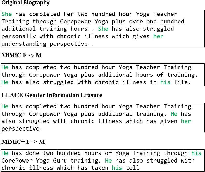
See fig 1 and Appendix D for a sample of the original and counterfactual sentences. The most salient change is in the usage of pronouns, where, as expected, when using MiMiC pronouns like “his”, “him” and “he” become much more frequent in the $\texttt{f}\to\texttt{m}$ direction, and vice versa. When using LEACE, sentences often exhibit pronouns mixing, wherein “he”, “she”, “his” and her” are used interchangeably. Less frequently, the phrase “he/she” is used. Beyond pronouns, we find that some more subtle changes sometimes occur, reflecting biases in the dataset. For instance, in the direction $\texttt{m}\to\texttt{f}$ the counterfactuals of the biographies of doctors often omit the “Dr.” prefix and replace it with “Ms”. The enhanced counterfactuals of $\texttt{MiMiC}^{+}_{\alpha}$ exhibit an over-usage of stereotypical markers of the target gender, adding pronouns when they are not necessary or introducing new stereotypical information. This intervention tends to modify further the overall structure of the sentence. The inversion process is not perfect, and at times inflicts some changes to the original text, such as paraphrasing.

Word frequency analysis.

To quantitatively evaluate the more subtle changes entailed by the counterfactual generation process, we analyze the word whose probabilities change the most between the original and counterfactual sentences. Specifically, we calculate the following score to quantify changes in unigram probabilities:

\Delta=\frac{p(\text{w}\mid\text{G})-p(\text{w}\mid\text{G}^{\text{counterfactual}})}{p(\text{w}\mid\text{G})-p(\text{w}\mid\text{G}^{\text{counterfactual}}_{\text{no-intervention}})+1}

(1)

Where G is a group of original sentences (e.g., biographies of males), $\text{G}^{\text{counterfactual}}$ is their counterfactual counterpart (e.g., in the $\texttt{m}\to\texttt{f}$ direction), and $\text{G}^{\text{counterfactual}}_{\text{no-intervention}}$ is the counterfactuals that are generated without an intervention. We then sort the vocabulary by the $\Delta$ score and record the words whose probabilities increase or decrease the most relative to the counterfactuals generated without an intervention. We omit words whose frequency in either group is less than 10. This analysis is conducted on the MiMiC counterfactuals.

Results. See Appendix B for the most-changed words. As anticipated, in the $\texttt{f}\to\texttt{m}$ direction, the frequency of “he” and “his” experiences the most significant increase, whereas in the $\texttt{m}\to\texttt{f}$ direction, these shifts are observed with the words “she” and “her”. Beyond pronouns, there is a discernible change in the frequency of prepositions: “of” and “the” emerge as the 3rd and 4th words that become more prevalent in the $\texttt{f}\to\texttt{m}$ direction, alongside “a”, “at”, and “for”. This phenomenon aligns with a recognized bias where male authors tend to utilize articles and certain prepositions more heavily Koppel et al. (2002); Schler et al. (2006). Concerning content words, specific terms associated with a “professional” context, such as “medical”, “university”, “featured”, “member”, and “finalist”, exhibit increased frequency in the $\texttt{f}\to\texttt{m}$ direction, while words like “affiliated”, “dr”, “surgery”, and “received” (often a degree) decrease in frequency in the $\texttt{m}\to\texttt{f}$ direction.³³3This trend is not entirely consistent, with some “professional” words such as “specializes” and “education” becoming more frequent in the $\texttt{m}\to\texttt{f}$ direction.

Human evaluation

We perform human annotation on a sample of sentences in order to answer 2 questions: (1) whether the counterfactual intervention entails a damage to the writing quality of the biography (beyond that which is entailed by the inversion process without intervention), and (2) whether the counterfactual intervention is successful in inverting the property we focus on. Superficially, to answer question (1) we ask annotators to compare the writing quality of pairs of sentences, where one of the three interventions was applied followed by decoding to the natural language space, alongside the corresponding decoded sentence without intervention. See Appendix C for the complete annotation process and results. We find that the interventions did not significantly affect the overall writing quality of the sentences, while it indeed transformed the subject entity pronouns almost perfectly using the MiMiC methods. LEACE , an erasure method, induced a random usage of pronouns (Fig. 1).

4.2 Increasing Fairness by Counterfactual Data Augmentation

The BiasBios data exhibits an imbalance in the representation of men and women across various professions, leading to observed biases in profession classifiers trained on this data De-Arteaga et al. (2019). In this experiment, we make use of the counterfactuals we generate for data augmentation. By adding counterfactual examples with the opposite gender label, we expect to mitigate the model’s dependence on gender.

Setup

We embed each biography by the last layer representation of a GTR-base model Ni et al. (2021). Subsequently, an intervention is applied, followed by decoding the intervened representation using the trained inversion model. A beam size width of 4 was employed, along with 20 correction steps using the pre-trained Natural Questions corrector from Morris et al. (2023). This pipeline repeats for the three intervention techniques: LEACE, MiMiC, and $\texttt{MiMiC}^{+}_{\alpha}$ . Results are averaged over 3 models (see Appendix A). Following previous work De-Arteaga et al. (2019) we quantify bias by the mean True Positive Rate (TPR) gap of a profession classifier between genders.

Models

We train Roberta-base profession classifiers Liu et al. (2019). We consider the following baselines: training on the original biographies, on the reconstructed biographies without an intervention ( $\color[rgb]{0,0,0}\definecolor[named]{pgfstrokecolor}{rgb}{0,0,0}\pgfsys@color@gray@stroke{0}\pgfsys@color@gray@fill{0}{\texttt{inv}}(\color[rgb]{0,0,0}\definecolor[named]{pgfstrokecolor}{rgb}{0,0,0}\pgfsys@color@gray@stroke{0}\pgfsys@color@gray@fill{0}{\texttt{enc}}(\boldsymbol{{\color[rgb]{0,0,0}\definecolor[named]{pgfstrokecolor}{rgb}{0,0,0}\pgfsys@color@gray@stroke{0}\pgfsys@color@gray@fill{0}\mathrm{\color[rgb]{0,0,0}\definecolor[named]{pgfstrokecolor}{rgb}{0,0,0}\pgfsys@color@gray@stroke{0}\pgfsys@color@gray@fill{0}{T}}}}))$ ), and on a variant of the original dataset where explicit gender indicators (pronouns and names) are removed (“Biographies without gender indication” in Table 1). Finally, to test our method, we train a classifier on a dataset containing the original and counterfactual texts.⁴⁴4Note that in case of MiMiC and $\texttt{MiMiC}^{+}_{\alpha}$ , assuming the counterfactual generation process is successful, this ensures that the representation of males and females is equal overall and within each profession in the dataset.

Results

The results are presented in Table 1. Classifiers trained on the augmented dataset achieve lower TPR values (better fairness), even more so than classifiers trained on the biographies after the omission of overt gender markers.

5 Conclusions

We show it is possible to invert representation-space counterfactuals back into the input space (natural language). We confirm the high quality of the resultant counterfactual texts and illustrate their effectiveness in bias mitigation. Future work should explore the potential utility of these counterfactuals for causal effect estimation of natural-language interventions Feder et al. (2022).

Limitations

Quality of the inversion model

Our counterfactual generation pipeline relies on two components: the interventions and the inversion models. We aimed to disentangle these two factors in our evaluation by comparing the counterfactuals generated with the interventions with the counterfactuals without intervention. However, a complete disentanglement of these two factors is difficult, and it is possible that some of the changes we witness should be attributed to a non-perfect inversion process, rather than to the intervention. We observe that the inversion model is indeed not perfect, and often introduce slight variations in the text (e.g., by modifying numbers or geographical locations, or introducing lexical paraphrases). These changes might be undesired in certain use cases. However, an improvement in the inversion model is orthogonal to our method.

Causal interventions

As the generative process of natural language texts is opaque, we inevitably rely on markers that people often identify with the property of interest (gender) in our evaluation. Future work should use controlled, synthetic setting to test the degree to which the counterfactuals reflect the true causal factors related to the concept of interest.

Representation of gender

We inevitably use existing a dataset with binary gender labels. We acknowledge that this is a simplification, as gender is a complex nonbinary construct.

Ethical Considerations

In all scenarios involving the potential application of automated methods in real-world contexts, we strongly recommend exercising caution and conducting thorough assessments of the data’s representativeness, its alignment with real-world phenomena, and possible adverse societal implications. Gender bias is a multifaceted and intricate issue, and we view the experiments conducted in this paper as an initial exploration into strategies for mitigating the negative impacts of LMs, rather than a definitive solution to real-world bias challenges. As highlighted in the limitations section, the utilization of binary gender labels arises from limitations in available data, and we anticipate that future research will facilitate more nuanced examinations of how gender, as a construct, manifests in text.

References

Belrose et al. (2023) Nora Belrose, David Schneider-Joseph, Shauli Ravfogel, Ryan Cotterell, Edward Raff, and Stella Biderman. 2023. Leace: Perfect linear concept erasure in closed form. arXiv preprint arXiv:2306.03819.
Bolukbasi et al. (2016) Tolga Bolukbasi, Kai-Wei Chang, James Y. Zou, Venkatesh Saligrama, and Adam Tauman Kalai. 2016. Man is to computer programmer as woman is to homemaker? debiasing word embeddings. In Advances in Neural Information Processing Systems 29: Annual Conference on Neural Information Processing Systems 2016, December 5-10, 2016, Barcelona, Spain, pages 4349–4357.
De-Arteaga et al. (2019) Maria De-Arteaga, Alexey Romanov, Hanna Wallach, Jennifer Chayes, Christian Borgs, Alexandra Chouldechova, Sahin Geyik, Krishnaram Kenthapadi, and Adam Tauman Kalai. 2019. Bias in bios: A case study of semantic representation bias in a high-stakes setting. In proceedings of the Conference on Fairness, Accountability, and Transparency, pages 120–128.
De-Arteaga et al. (2019) Maria De-Arteaga, Alexey Romanov, Hanna M. Wallach, Jennifer T. Chayes, Christian Borgs, Alexandra Chouldechova, Sahin Cem Geyik, Krishnaram Kenthapadi, and Adam Tauman Kalai. 2019. Bias in bios: A case study of semantic representation bias in a high-stakes setting. CoRR, abs/1901.09451.
Elazar et al. (2021) Yanai Elazar, Shauli Ravfogel, Alon Jacovi, and Yoav Goldberg. 2021. Amnesic probing: Behavioral explanation with amnesic counterfactuals. Transactions of the Association for Computational Linguistics, 9:160–175.
Feder et al. (2022) Amir Feder, Katherine A Keith, Emaad Manzoor, Reid Pryzant, Dhanya Sridhar, Zach Wood-Doughty, Jacob Eisenstein, Justin Grimmer, Roi Reichart, Margaret E Roberts, et al. 2022. Causal inference in natural language processing: Estimation, prediction, interpretation and beyond. Transactions of the Association for Computational Linguistics, 10:1138–1158.
Fleiss (1971) Joseph L Fleiss. 1971. Measuring nominal scale agreement among many raters. Psychological bulletin, 76(5):378.
Geva et al. (2021) Mor Geva, Roei Schuster, Jonathan Berant, and Omer Levy. 2021. Transformer feed-forward layers are key-value memories. In Proceedings of the 2021 Conference on Empirical Methods in Natural Language Processing, pages 5484–5495.
Guerner et al. (2023) Clément Guerner, Anej Svete, Tianyu Liu, Alexander Warstadt, and Ryan Cotterell. 2023. A geometric notion of causal probing. arXiv preprint arXiv:2307.15054.
Koppel et al. (2002) Moshe Koppel, Shlomo Argamon, and Anat Rachel Shimoni. 2002. Automatically categorizing written texts by author gender. Literary and linguistic computing, 17(4):401–412.
Kwiatkowski et al. (2019) Tom Kwiatkowski, Jennimaria Palomaki, Olivia Redfield, Michael Collins, Ankur Parikh, Chris Alberti, Danielle Epstein, Illia Polosukhin, Jacob Devlin, Kenton Lee, et al. 2019. Natural questions: a benchmark for question answering research. Transactions of the Association for Computational Linguistics, 7:453–466.
Li et al. (2023) Kenneth Li, Oam Patel, Fernanda Viégas, Hanspeter Pfister, and Martin Wattenberg. 2023. Inference-time intervention: Eliciting truthful answers from a language model. arXiv preprint arXiv:2306.03341.
Liu et al. (2019) Yinhan Liu, Myle Ott, Naman Goyal, Jingfei Du, Mandar Joshi, Danqi Chen, Omer Levy, Mike Lewis, Luke Zettlemoyer, and Veselin Stoyanov. 2019. Roberta: A robustly optimized bert pretraining approach. arXiv preprint arXiv:1907.11692.
Morris et al. (2023) John X Morris, Volodymyr Kuleshov, Vitaly Shmatikov, and Alexander M Rush. 2023. Text embeddings reveal (almost) as much as text. arXiv preprint arXiv:2310.06816.
Ni et al. (2021) Jianmo Ni, Chen Qu, Jing Lu, Zhuyun Dai, Gustavo Hernández Ábrego, Ji Ma, Vincent Y Zhao, Yi Luan, Keith B Hall, Ming-Wei Chang, et al. 2021. Large dual encoders are generalizable retrievers. arXiv preprint arXiv:2112.07899.
Pearl (1988) Judea Pearl. 1988. Probabilistic reasoning in intelligent systems: networks of plausible inference. Morgan kaufmann.
Ravfogel et al. (2020) Shauli Ravfogel, Yanai Elazar, Hila Gonen, Michael Twiton, and Yoav Goldberg. 2020. Null it out: Guarding protected attributes by iterative nullspace projection. In Proceedings of the 58th Annual Meeting of the Association for Computational Linguistics, pages 7237–7256.
Ravfogel et al. (2021) Shauli Ravfogel, Grusha Prasad, Tal Linzen, and Yoav Goldberg. 2021. Counterfactual interventions reveal the causal effect of relative clause representations on agreement prediction. In Proceedings of the 25th Conference on Computational Natural Language Learning, pages 194–209.
Ravfogel et al. (2022) Shauli Ravfogel, Francisco Vargas, Yoav Goldberg, and Ryan Cotterell. 2022. Adversarial concept erasure in kernel space. arXiv preprint arXiv:2201.12191.
Schler et al. (2006) Jonathan Schler, Moshe Koppel, Shlomo Argamon, and James W Pennebaker. 2006. Effects of age and gender on blogging. In AAAI spring symposium: Computational approaches to analyzing weblogs, volume 6, pages 199–205.
Singh et al. (2024) Shashwat Singh, Shauli Ravfogel, Jonathan Herzig, Roee Aharoni, Ryan Cotterell, and Ponnurangam Kumaraguru. 2024. Mimic: Minimally modified counterfactuals in the representation space.
Subramani et al. (2022) Nishant Subramani, Nivedita Suresh, and Matthew E Peters. 2022. Extracting latent steering vectors from pretrained language models. In Findings of the Association for Computational Linguistics: ACL 2022, pages 566–581.

Appendix

Appendix A Experimental setup

Training an inversion model

Morris et al. (2023) introduced an approach for inverting static embeddings back into text. To effectively invert the embeddings derived from the BiasBios dataset, we trained a dedicated inversion model on sequences with a length of 64 tokens from the Natural Questions dataset Kwiatkowski et al. (2019). This decision was informed by the observation that the median biography length within the BiasBios dataset is 72 tokens. The model architecture is GTR-base (Ni et al., 2021) as used originally in vec2text Morris et al. (2023). Our training procedure entailed 50 epochs on the Natural Questions dataset, succeeded by fine-tuning for an additional 10 epochs on the BiasBios dataset.

Training profession classifiers

To quantify the counterfactuals causal effect on predicting person’s profession, we trained a Roberta classifiers (Liu et al., 2019). We trained each classifier with 3 different seeds, reporting the mean score of the models with the lowest validation loss. Each classifier was trained for 10 epochs on the entire BiasBios biographies with a length within 64 tokens, leaving 41,563 male biographies and 36,148 biographies, where the train set of the counterfactual classifiers include for each sample its corresponding counterfactual. We used a batch size of 1024 samples for training and 4096 for evaluation, 6% of the samples were used for warmup up to a 2e-5 learning rate, we also utilized half precision quantization, i.e., fp16. The results reported at 1 were calculated on the entire BiasBios test set, i.e., 98,344 samples, truncated to a 64 tokens sequence length.

Appendix B Word Frequency Analysis

We provide here the words most changed due to the MiMiC intervention:

•

words whose probabilities most decreased in direction $\texttt{m}\to\texttt{f}$ : [’he’, ’his’, ’the’, ’mr.’, ’&’, ’of’, ’blue’, ’him’, ’for’, ’university’, ’affiliated’, ’dr’, ’at’, ’insurance’, ’-’, ’include’, ’many’, ’surgery’, ’years’, ’various’, ’shield’, ’average’, ’received’, ’out’, ’this’]
•

words whose probabilities most increased in direction $\texttt{m}\to\texttt{f}$ : [’she’, ’her’, ’in’, ’to’, ’a’, ’as’, ’is’, ’and’, ’currently’, ’community’, ’featured’, ’been’, ’an’, ’was’, ’health’, ’specializes’, ’listed’, ’national’, ’where’, ’one’, ’education’, ’help’, ’that’, ’who’, ’ms’]
•

words whose probabilities most decreased in direction $\texttt{f}\to\texttt{m}$ : [’she’, ’her’, ’ms.’, ’and’, ’in’, ’listed’, ’currently’, ’with’, ’on’, ’freeones’, ’is’, ’medicine’, ’practices’, ’ranked’, ’affiliated’, ’2014’, ’154th’, ’gallery’, ’to’, ’since’, ’health’, ’freeones.’, ’&’, ’born’, ’children’]
•

words whose probabilities most increased in direction $\texttt{f}\to\texttt{m}$ : [’he’, ’his’, ’of’, ’the’, ’dr.’, ’mr.’, ’a’, ’for’, ’at’, ’has’, ’medical’, ’him’, ’many’, ’been’, ’university’, ’freeone’, ’featured’, ’member’, ’various’, ’one’, ’number’, ’blue’, ’by’, ’finalist’, ’this’]

Appendix C Human annotation

We conducted human annotation experiments to evaluate the quality of the interventions. The annotation was conducted by 3 STEM students, who volunteered for this task. The annotators were required to complete 2 tasks: (1) assessing the writing quality of pairs of sentences, and (2) determining the subject entity gender for a list of sentences. An agreement between the annotators was measured by Fleiss Kappa score Fleiss (1971). The Fleiss Kappa for the first task, i.e., comparing the writing quality of the sentences pair was 0.1955, and for the second task, determining the subject entity gender was 0.915. To isolate the quality degradation induced by the inversion model, task (1) comprising pairs of decoded sentences without intervention, alongside the same sentence with intervention applied at the representational space prior to decoding. The samples were drawn randomly using a random sample generator. The exact instructions are given below. {spverbatim} Task 1: You are given 6 files with pairs of sentences and asked to annotate which one is better in terms of writing quality. Mark 1 if sentence 1 has better writing quality compared to sentence 2, Mark 2 if sentence 2 has better writing quality compared to 1, Mark 0 if both sentences have the same writing quality. Task2: You are given 6 files containing a list of sentences. Your objective is to determine the gender of the subject entity in each sentence. You have three options to choose from: female, male, or unclear.

C.1 Human Annotation Results

The complete human evaluation results are presented in Table 2 and Table 3. The great majority of counterfactuals contain pronouns that match the target class. LEACE-an erasure method–induces in 16%-28% of the cases a mixture of pronoun types within the same text. On the other cases, the pronouns form the two classes are roughly equally divided, i.e, the method randomly substitutes some of the pronouns with pronouns from the other class. When it comes to writing quality, we see some degradation in quality following the intervention (Table 3), although in the majority of cases the annotators did not favor either of the versions.

Method	Perceived gender markers
	f	m	Unclear
MiMiC $\texttt{f}\to\texttt{m}$	0.04 $\pm 0$	0.96 $\pm 0$	0 $\pm 0$
MiMiC $\texttt{m}\to\texttt{f}$	0.96 $\pm 0$	0 $\pm 0$	0.04 $\pm 0$
$\texttt{MiMiC}^{+}_{\alpha}$ $\texttt{f}\to\texttt{m}$	0 $\pm 0$	0.96 $\pm 0.04$	0.04 $\pm 0$
$\texttt{MiMiC}^{+}_{\alpha}$ $\texttt{m}\to\texttt{f}$	1 $\pm 0$	0 $\pm 0$	0 $\pm 0$
LEACE (Originally f)	0.44 $\pm 0.0692$	0.4 $\pm 0.0692$	0.16 $\pm 0.1385$
LEACE (Originally m)	0.32 $\pm 0$	0.4 $\pm 0$	0.28 $\pm 0$

Table 2: Evaluating the success rate of the counterfactual generation

Setting	Decoded+intervention quality $>$ Decoded quality	Decoded quality $>$ Decoded + intervention quality	Same quality
LEACE	0.0733 $\pm$ 0.0702	0.1538 $\pm$ 0.0693	0.7727 $\pm$ 0.1396
MiMiC	0.0868 $\pm$ 0.133	0.1804 $\pm$ 0.1106	0.7327 $\pm$ 0.1795
$\texttt{MiMiC}^{+}_{\alpha}$	0.0802 $\pm$ 0.0526	0.3013 $\pm$ 0.0848	0.6183 $\pm$ 0.1285

Table 3: Human annotation results, measuring the writing quality of pairs of intervened sentences and the decoded sentence without intervention.

Appendix D Intervention inversion sample

In Table 4 we provide a random sample of the counterfactuals generated by the different methods.

Method	Inversion without intervention	Intervention + Inversion
MiMiC $\texttt{f}\to\texttt{m}$	she graduated from Southeastern Oklahoma University with a Bachelor’s degree in Business Administration in 2005. Chandra has worked in public accounting in both the state	with a Bachelor of Business Administration. Chandra graduated from Southeastern Oklahoma University in 2007. He has worked in a number of public accounting firms including Texas
MiMiC $\texttt{f}\to\texttt{m}$	She was born in Tokyo in October 1995. She is currently listed on FreeOnes and has been ranked 157th in 2013 for her entries.	he was born in Tokyo in October 1999. He has been ranked 3rd in the FreeOne International Collection and 5th in the Asian Studies
MiMiC $\texttt{m}\to\texttt{f}$	His family are long time members of First Universalist Church of Pittsfield. His poetry reflects his deep appreciation for Nature and our intuition and experience.	Her family are members of First Universalist Church of Pittsfield. Her poetry reflects great appreciation for nature along with deep intuition and deep experiences. Together
MiMiC $\texttt{m}\to\texttt{f}$	His early 70s work has continued into the 21st century where his film career has yet to flourish. He has won many Oscar, Broadway awards and	Her Broadway career has spanned many decades from the late ’50s until the present. Her work has been awarded a 1977 Oscar more
LEACE (Originally female)	She has also taught previous courses on LSAT Procedure Preparedness and has led panel discussions on new contracts and activities for Oregon bar and state lawyers. This	She has taught courses on LSAT Procedure Preparedness for current and future lawyers, as well as panel discussions on contract proposals and activities for Oregon bar associations
LEACE (Originally female)	She began her career working in Bolivia where her mother lived in the United States. She has an organization called Dream Latino and now promotes Zoom on CNN	began her career working for Dream Zoom in the United States. She has a division in Bolivia called "Mom Latino" where she interviewed news
LEACE (Originally male)	when not playing guitar he spends the majority of his time with the family and is watching rugby, teaching maths etc. and writing codes.â€™	When she is not writing or teaching maths he spends most of her time with her family - watching rugby and playing guitar / all codes
LEACE (Originally male)	He is a co-author of: Media Economics Theory & Practices. Recent research includes: Assessing the social impact of online communication and technology	theory and research. He is author of Media Economics: A New Approach to Recognising the social impact of online technologies on online communication. As of
$\texttt{MiMiC}^{+}_{\alpha}$ $\texttt{f}\to\texttt{m}$	Crystal Yang received a research grant for UND as a way to participate in cutting arts in Beijing. Wang went to Hong Kong for the December 2009	Art and Engineering Grant from UND for Wang Yang. He received a lot of money for his work in Crystal when he was visiting Beijing in April
$\texttt{MiMiC}^{+}_{\alpha}$ $\texttt{f}\to\texttt{m}$	She has received a multimillion dollar Queensland hospital community recognition in 2007 for writing and contributing to both public and media investigative reporting. In the mid-19	been a bit of a pioneer of his specialised reporting and investigative writing. He has been awarded $2 million by the Queensland Media Forum in 2007,
$\texttt{MiMiC}^{+}_{\alpha}$ $\texttt{m}\to\texttt{f}$	served as a partner in the Rotary Club of East Sacramento. In October 2013, Bob was elected to head up District 5180. In April and May 2014	In August 2007, she was elected to District 599. In May 2017, she helped the Sacramento Rotary Club guide women to a life of their own. She
$\texttt{MiMiC}^{+}_{\alpha}$ $\texttt{m}\to\texttt{f}$	In addition to saxophone he teaches truman and woodwind classes. Dr. Smith taught instrumental music at Three Rivers	- She teaches sax and woodwind. In addition to instrumental music, Dr. Smith taught 3 Rivers community classes at Truman

Table 4: Random sample of inverted representations without intervention, alongside an intervention + inversion.