Probabilistic Routing for Graph-Based
Approximate Nearest Neighbor Search

Abstract

Approximate nearest neighbor search (ANNS) in high-dimensional spaces is a pivotal challenge in the field of machine learning. In recent years, graph-based methods have emerged as the superior approach to ANNS, establishing a new state of the art. Although various optimizations for graph-based ANNS have been introduced, they predominantly rely on heuristic methods that lack formal theoretical backing. This paper aims to enhance routing within graph-based ANNS by introducing a method that offers a probabilistic guarantee when exploring a node’s neighbors in the graph. We formulate the problem as probabilistic routing and develop two baseline strategies by incorporating locality-sensitive techniques. Subsequently, we introduce PEOs, a novel approach that efficiently identifies which neighbors in the graph should be considered for exact distance computation, thus significantly improving efficiency in practice. Our experiments demonstrate that equipping PEOs can increase throughput on a commonly utilized graph index (HNSW) by a factor of 1.6 to 2.5, and its efficiency consistently outperforms the leading-edge routing technique by 1.1 to 1.4 times.

1 Introduction

Nearest neighbor search (NNS) is the process of identifying the vector in a dataset that is closest to a given query vector. This technique has found widespread application in machine learning, with numerous solutions to NNS having been proposed. Given the challenge of finding exact answers, practical efforts have shifted towards approximate NNS (ANNS) for efficiency. While some approaches provide theoretical guarantees for approximate answers – typically through locality-sensitive hashing (LSH) [7, 11, 3] – others prioritize faster search speeds for a desired recall level by utilizing quantization [21, 16] or graph indexes [25, 14].

Graph-based ANNS, distinguished by its exceptional empirical performance, has become the leading method for ANNS and is widely implemented in vector search tools and databases. During the indexing phase, graph-based ANNS constructs a proximity graph where nodes represent data vectors and edges connect closely located vectors. In the search phase, it maintains a priority queue and a result list while exploring the graph. Nodes are repeatedly popped from the priority queue until it is empty, computing the distance from their neighbors to the query. Neighbors that are closer than the furthest element in the result list are added to the queue, and the results are accordingly updated.

To further improve the performance of graph-based ANNS, practitioners have introduced various empirical optimization techniques, including routing [34, 26, 5, 8], edge selection [13, 31], and quantization [24, 20]. The primary objective is to minimize distance computations during neighbor exploration. However, most of these optimizations are heuristic, based on empirical observations (e.g., over 80% of data vectors are less relevant than the furthest element in the results list and thus should be pruned before exact distance computations [8]), making them challenging to quantitatively analyze. Although analyses elucidate the effectiveness of graph-based ANNS [29, 19], they concentrate on theoretical aspects rather than empirical improvements.

In this paper, we investigate routing in graph-based ANNS, aiming to identify which neighbors should be evaluated for distance to the query during the search phase efficiently. Our objective is to bridge the theoretical and practical aspects of ANNS by providing a theoretical guarantee. While achieving an LSH-like guarantee for graph-based ANNS is challenging, we demonstrate that it is feasible to establish a probabilistic guarantee for exploring a node’s neighbors. Specifically, we introduce probabilistic routing in graph-based ANNS: for a given top node $v$ in the priority queue, an error bound $\epsilon$, and a distance threshold $\delta$, any neighbor $u$ of $v$ with a distance to the query less than $\delta$ will be computed for distance with a probability of at least $1-\epsilon$. Addressing the probabilistic routing problem yields several benefits: First, it ensures that ANNS explores the most promising neighbors (less than 20% of all neighbors, as observed in [8]) with high probability, facilitates quantitative analysis of a search algorithm’s effectiveness. Second, by devising probabilistic routing algorithms that accurately and efficiently estimate distances, we can significantly enhance practical efficiency. Third, the theoretical framework ensures consistent performance across different datasets, contrasting with heuristic approaches that may result in high estimation errors and consequently, lower recall rates.

To address the probabilistic routing problem, we initially integrate two foundational algorithms from existing research – SimHash [7] and (reverse) CEOs [27] – into graph-based ANNS. Subsequently, we introduce a novel routing algorithm, namely Partitioned Extreme Order Statistics (PEOs), characterized by the following features:

(1) PEOs utilizes space partitioning and random projection techniques to estimate a random variable which represents the angle between each neighbor and the query vector. By aggregating projection data from multiple subspaces, we substantially reduce the variance of the estimated random variable’s distribution, thereby enhancing the accuracy of neighbor-to-query distance estimations.

(2) Through comprehensive analysis, we show that PEOs addresses the probabilistic routing problem within a user-defined error bound $\epsilon$ ($\epsilon\leq 0.5$). The algorithm introduces a parameter $L$, denoting the number of subspaces in partitioning. An examination of $L$’s influence on routing enables us to identify an optimal parameter configuration for PEOs. Comparative analysis with baseline algorithms reveals that an appropriately selected $L$ value yields a variance of PEOs’ estimated random variable than that obtained via SimHash-based probabilistic routing and the reverse CEOs-based probabilistic routing is a special case of PEOs with $L=1$.

(3) The implementation of PEOs is optimized using pre-computed data and lookup tables, facilitating fast and accurate estimations. The use of SIMD further enhances processing speed, allowing for the simultaneous estimation of 16 neighbors and leveraging the data locality, a significant improvement over conventional methods that require accessing raw vector data stored disparately in memory.

Our empirical validation encompasses tests on six publicly accessible datasets. By integrating PEOs with HNSW [25], the predominant graph index for ANNS, we achieve a reduction in the necessity for exact distance computations by 70% to 80%, thereby augmenting queries per second (QPS) rates by 1.6 to 2.5 times under various recall criteria. Moreover, PEOs demonstrates superior performance to FINGER [8], a leading-edge routing technique, consistently enhancing efficiency by 1.1 to 1.4 times while reducing space requirements.

2 Related Work

Various types of ANNS approaches have been proposed, encompassing tree-based approaches [9], hashing-based approaches [2, 22, 1, 3, 28], quantization based approaches [21, 16, 4, 17, 32], learn-to-index-based approaches [18, 23], and graph-based approaches [25, 31, 14, 13]. Among these, graph-based methods are predominantly considered state-of-the-art (SOTA). To enhance the efficiency of graph-based ANNS, optimizations can be broadly categorized into: (1) routing, (2) edge-selection, and (3) quantization, with these optimizations generally being orthogonal to one another. Given our focus on routing, we briefly review relevant studies in this domain. TOGG-KMC [34] and HCNNG [26] employ KD trees to determine the direction of the query, thereby restricting the search to vectors within that specified direction. Despite fast estimation, it tends to yield suboptimal query accuracy, limiting its effectiveness. FINGER [8] estimates the distance of each neighbor to the query. Specifically, for each node, it generates promising projected vectors locally to establish a subspace, and then applies collision counting, as in SimHash, to approximate the distance in each visited subspace. Learn-to-route [5] learns a routing function, utilizing additional representations to facilitate optimal routing from the starting node to the nearest neighbor.

3 Problem Definition

Definition 3.1 (Nearest Neighbor Search (NNS)).

Given a query vector $\bm{q}\in\mathbb{R}^{d}$ and a dataset of vectors $\mathcal{O}$, find the vector $\bm{o}^{\ast}\in\mathcal{O}$ such that $dist(\bm{q},\bm{o}^{\ast})$ is the smallest.

For distance function $dist(\cdot,\cdot)$, two widely utilized metrics are $\ell_{2}$ distance and angular distance. Maximum inner product search (MIPS), closely related to NNS, aims to identify the vector that yields the maximum inner product with the query vector. We elaborate on extension to MIPS in Appendix C.1 and plan to assess its performance in future work.

There is a significant interest not only in identifying a singular nearest neighbor but also in locating the top-$K$ nearest neighbors, a task referred to as $K$-NN search. It is a prevailing view that computing exact NNS results poses a considerable challenge, whereas determining approximate results suffices for addressing many practical applications [30]. Notably, many SOTA ANNS algorithms leverage a graph index, where each vector in $\mathcal{O}$ is linked to its nearby vectors.

Input : Query $\bm{q}$, # results $K$, graph index $G$

Output : $K$-NN of $\bm{q}$

$R\leftarrow\emptyset$ ;

  /* an ordered list of results, $|R|\leq efs$ */

$P\leftarrow\{\,$ entry node $v_{0}\in G\,\}$ ;

  /* a priority queue */

1 while $P\neq\emptyset$ do

2       $v\leftarrow P.pop()$;

3       foreach unvisited neighbor $u$ of $v$ do

4             if $|R|<efs$ then $\delta\leftarrow\infty$;

5             else $p\leftarrow R[efs]$, $\delta\leftarrow dist(\bm{p},\bm{q})$;

6             if RoutingTest($\bm{u},\bm{v},\bm{q},\delta$) = true then

7                   if $dist(\bm{u},\bm{q})<\delta$ then

8                         $R.push(u)$, $P.push(u)$;

9                        

10                  

11            

12      

return ($\{\,R[1],\ldots,R[K]\,\}$)

Algorithm 1 Graph-based ANNS with routing

The construction of a graph index can be approached in various ways, e.g., through a KNN graph [12], HNSW [25], NSG [14], and the improved variant NSSG [13]. Among these, HNSW stands out as the most extensively adopted model, implemented in many ANNS platforms such as Faiss and Milvus. Given a graph index $G=(V,E)$ built upon $\mathcal{O}$, traversal of this graph enables the discovery of ANNS results, as delineated in Algorithm 1. The search initiates from an entry node $v_{0}\in G$, maintaining $R$, an ordered list that contains no more than $efs$ ($efs\geq K$) – a list size parameter – results identified thus far. Neighbors of the entry node in the graph are examined against $\bm{q}$ for proximity and added to a priority queue if they are closer to the query than the most distant element in $R$ or if $R$ is not full. Nodes are popped from the priority queue to further explore their adjacent nodes in the graph, until the priority queue becomes empty. It is noteworthy that practical search operations may extend beyond those depicted in Algorithm 1, e.g., by employing pruning strategies to expedite the termination of the search process [25]. Algorithms designed for graph-based ANNS with angular distance can be adapted to accommodate $\ell_{2}$ distance, since calculating the $\ell_{2}$ distance between $\bm{q}$ and $\bm{o}\in\mathcal{O}$ merely involves determining the angle between them during graph traversal: $\ell_{2}(\bm{q},\bm{o})^{2}=\|\bm{q}\|^{2}+\|\bm{o}\|^{2}-2\bm{q}^{\top}\bm{o}$, where $\|\bm{q}\|$ is fixed and $\|\bm{o}\|$ can be pre-computed.

While naive graph exploration entails computing the exact distance for all neighbors, a routing test can be applied to assess whether a neighbor warrants exact distance computation. An efficient routing algorithm can substantially enhance the performance of graph-based ANNS. We study routing algorithms with the following probability guarantee.

Definition 3.2 (Probabilistic Routing).

Given a query vector $\bm{q}$, a node $v$ in the graph index, an error bound $\epsilon$, and a distance threshold $\delta$, for an arbitrary neighbor $u$ of $v$ such that $dist(\bm{u},\bm{q})<\delta$, if a routing algorithm returns true for $u$ with a probability of at least $1-\epsilon$, then the algorithm is deemed to be $(\delta,1-\epsilon)$-routing.

Given our interest in determining whether a neighbor has the potential to refine the temporary results, our focus narrows to the case when $\delta$ equals the distance between $\bm{q}$ and the most distant element in the result list $R$, with $|R|=efs$ (Lines 1 – 1, Algorithm 1).

4 Baseline Algorithms

To devise a baseline algorithm for probabilistic routing, we adapt SimHash [7] and CEOs [27] for routing test, which were designed for the approximation with recall guarantee for ANNS and MIPS, respectively.

4.1 SimHash Test

SimHash, a classical random projection-based LSH method for the approximation of angular distance, has the following result [7].

Lemma 4.1.

(SimHash) Given $\bm{u}$, $\bm{q}$, and $m$ random vectors $\{\,\bm{a}_{i}\,\}^{m}_{i=1}\sim\mathcal{N}(0,I^{d})$, the angle $\theta$ between $\bm{u}$ and $\bm{q}$ can be estimated as

$$\hat{\theta}=\frac{1}{{\pi m}}\sum\limits_{i}{[{\mathop{\rm sgn}}(\bm{u}^{\top}\bm{a}_{i})\neq{\mathop{\rm sgn}}(\bm{q}^{\top}\bm{a}_{i})]}.$$ (1)

Based on the above lemma, we design a routing test:

$${\rm{\textbf{SimHash}}}\;{\rm{\textbf{Test:}}}\quad\#Col(\bm{u},\bm{q})\geq T_{\epsilon}^{\text{SimHash}}(\bm{u},\bm{q},\delta,m)$$ (2)

where $\#Col$ denotes the collision number of the above random projection along $\{\,\bm{a}_{i}\,\}^{m}_{i=1}$, and $T_{\epsilon}^{\text{SimHash}}(\bm{u},\bm{q},\delta,m)$ denotes a threshold determined by $\epsilon$ and $\delta$. A neighbor $u$ of $v$ passes the routing test iff. it satisfies the above condition. By careful setting of the threshold, we can obtain the desired probability guarantee. Besides probabilistic routing, SimHash has also been used in FINGER [8] to speed up graph-based ANNS, serving as one of its building blocks but utilized in a heuristic way.

It can be seen that the result of the above SimHash test is regardless of $v$. This means that if a node $u$ fails in a test, it will never be inserted into the result set or the priority queue. Since this will compromise the recall of ANNS, we design the following remedy by regarding the neighbors of $v$ as residuals w.r.t. $v$: for each neighbor $u$ of $v$, let $\bm{e}=\bm{u}-\bm{v}$, and this residual can be associated with the edge $e$ from $v$ to $u$ in the graph index. $\bm{e}$ is then used instead of $\bm{u}$ in the SimHash test. As such, the routing test becomes dependent on $\bm{v}$, and a threshold $T_{\epsilon}^{\text{SimHash}}(\bm{u},\bm{v},\bm{q},\delta,m)$ can be derived by the Hoeffding’s inequality applied to the Binominal distribution. Hence a neighbor $u$ may fail to pass the test w.r.t. $v$ but succeed in the test w.r.t. node $v^{\prime}$ in the graph index. Moreover, to model the angle between $\bm{e}$ and $\bm{q}$ in the routing test, we normalize $\bm{q}$ to $\bm{q}^{\prime}$ (and optionally, $\bm{e}$ to $\bm{e}^{\prime}$) to simplify computation. We discuss algorithms in the context of the above remedy hereafter.

4.2 RCEOs Test

In the realm of LSH, Andoni et al. proposed Falconn [3] for angular distance whose basic idea is to find the closest or furthest projected vector to the query and record such vector as a hash value, leading to a better search performance than SimHash. Pham and Liu [28] employed Concomitants of Extreme Order Statistics (CEOs) [27] to record the minimum or maximum projection value, further improving the performance of Falconn. By swapping the roles of query and data vectors in CEOs, we have Reverse CEOs (RCEOs) and it can be applied to graph-based ANNS with probabilistic routing:

Lemma 4.2.

(RCEOs) Given two normalized vectors $\bm{e}^{\prime}$, $\bm{q}^{\prime}$, and $m$ random vectors $\{\bm{a}_{i}\}^{m}_{i=1}\sim\mathcal{N}(0,I^{d})$, and $m$ is sufficiently large, assuming that $\bm{a}_{1}={\mathop{\rm argmax}_{\bm{a}_{i}}}|\bm{e}^{\prime\top}\bm{a}_{i}|$, we have the following result:

$$\bm{q}^{\prime\top}\bm{a}_{1}\sim\mathcal{N}({\mathop{\rm sgn}}(\bm{e}^{\prime\top}\bm{a}_{1})\cdot\bm{e}^{\prime\top}\bm{q}^{\prime}\sqrt{2\ln m},1-(\bm{e}^{\prime\top}\bm{q}^{\prime})^{2}).$$ (3)

Despite an asymptotic result, it has been shown that $m$ does not need to be very large ($\geq 128$) to ensure an enough closeness to the objective normal distribution [27].

Based on Lemma 4.2, we design a routing test:

$${\rm{\textbf{RCEOs}}}\;{\rm{\textbf{Test:}}}\quad\bm{q}^{\prime\top}\bm{a}_{1}\geq T_{\epsilon}^{\text{RCEOs}}(\bm{u},\bm{v},\bm{q},\delta,m)$$ (4)

where $\bm{a}_{1}={\mathop{\rm argmax}_{\bm{a}_{i}}}|\bm{e}^{\prime\top}\bm{a}_{i}|$ and $T_{\epsilon}^{\text{RCEOs}}(\bm{u},\bm{v},\bm{q},\delta,m)$ denotes a threshold related to $\epsilon$ and $\delta$.

5 Partitioned Extreme Order Statistics (PEOs)

5.1 Space Partitioning

In PEOs, the data space is partitioned into $L$ subspaces. Let $M\subseteq\mathbb{R}^{d}$ be the original data space. We decompose $M$ into $L$ orthogonal $d^{\prime}$-dimensional subspaces $M_{1},M_{2},\ldots,M_{L}$, $d^{\prime}=d/L$. When $L>1$, we can significantly decrease the variance of the normal distribution in RCEOs ((3)), hence delivering a better routing test. Specifically, (1) RCEOs test is a special case of PEOs test with $L=1$, and (2) by choosing an appropriate $L$ ($L>1$), PEOs test outperforms SimHash test while RCEOs test cannot (Appendix B).

5.2 PEOs Test

Following the space partitioning, for each neighbor $u$ of $v$, $\bm{e}$ is partitioned to $[\bm{e}_{1},\bm{e}_{2},\ldots,\bm{e}_{L}]$, where $\bm{e}_{i}$ is the sub-vector of $\bm{e}$ in $M_{i}$. The PEOs test consists of the following steps.

(1) (Orthogonal Decomposition) We decompose $\bm{e}$ as $\bm{e}=\bm{e}_{reg}+\bm{e}_{res}$ such that $\bm{e}_{reg}\perp\bm{e}_{res}$ and the direction of $\bm{e}_{reg}$ is determined as follows:

$$\frac{\bm{e}_{reg}}{\|\bm{e}_{reg}\|}=[\frac{\bm{e}_{1}}{\sqrt{L}\|\bm{e}_{1}\|},\frac{\bm{e}_{2}}{\sqrt{L}\|\bm{e}_{2}\|},\ldots,\frac{\bm{e}_{L}}{\sqrt{L}\|\bm{e}_{L}\|}].$$ (5)

We call $\bm{e}_{reg}$ the regular part of $\bm{e}$ and $\bm{e}_{res}$ the residual part of $\bm{e}$. Besides, we introduce two weights $w_{reg}$ and $w_{res}$ such that $w_{reg}=\|\bm{e}_{reg}\|/\|\bm{e}\|$ and $w_{res}=\|\bm{e}_{res}\|/\|\bm{e}\|$.

(2) (Generating Projected Vectors) In each $M_{i}$, we independently generate $m$ projected vectors $\{\bm{a^{i}_{j}}\}^{m}_{j=1}$, where $\bm{a^{i}_{j}}\sim\mathcal{N}(0,I^{d^{\prime}\times d^{\prime}})$. In the original space $M$, we independently generate $m$ projected vectors $\{\bm{b_{j}}\}^{m}_{j=1}$ such that $\bm{b_{j}}\sim\mathcal{N}(0,I^{d\times d})$.

(3) (Collection of Extreme Values) In each $M_{i}$, we collect $L+1$ extreme values that yield the greatest inner products with the projected vectors: $e[i]={\rm{sgn}}(\bm{e}_{i}^{\top}\bm{a^{i}_{j}})j$, where $j=\mathop{\rm argmax}_{j}|\bm{e}_{i}^{\top}\bm{a^{i}_{j}}|$, and $e[0]={\rm{sgn}}(\bm{e}_{res}^{\top}\bm{b_{j}})j$, where $j=\mathop{\rm argmax}_{j}|\bm{e}_{res}^{\top}\bm{b_{j}}|$.

(4) (CDF of Normal Distribution) Let $\mathcal{N}^{\bm{e},x}_{\min}$ be the following normal distribution associated with $\bm{e}$:

$$\mathcal{N}^{\bm{e},x}_{\min}=\mathcal{N}(x\sqrt{2L\ln m},w_{reg}^{2}+Lw_{res}^{2}-\frac{Lx^{2}}{L+1})$$ (6)

where $0<x<1$. Let $F_{\bm{e},x}$ be the CDF of $\mathcal{N}^{\bm{e},x}_{\min}$. We define $F^{-1}_{\bm{e}}(x,z)$ such that $F_{\bm{e},x}(F^{-1}_{\bm{e}}(x,z))=z$, where $0<z\leq 0.5$. Note that $F^{-1}_{\bm{e}}$ can be well-defined since $F_{\bm{e},x}(z)$ is a monotone function of $x$ when $z$ is fixed. When setting $z=\epsilon$, we write $F^{-1}_{\bm{e},\epsilon}(x)=F^{-1}_{\bm{e}}(x,\epsilon)$.

(5) (Query Projection) Given query $\bm{q}$, we normalize it to $\bm{q}^{\prime}$ and compute the inner products with the projected vectors to obtain two values $H_{1}(\bm{e})$ and $H_{2}(\bm{e})$ w.r.t. $\bm{e}$:

$$H_{1}(\bm{e})=\sum\limits_{i}{\rm{sgn}}(e[i])(\bm{q}_{i}^{\prime\top}\bm{a}^{i}_{|e[i]|}),$$ (7)

$$H_{2}(\bm{e})={\rm{sgn}}(e[0])(\bm{q}^{\prime\top}\bm{b}_{|e[0]|}).$$ (8)

(6) (Routing Test) With $H_{1}(\bm{e})$ and $H_{2}(\bm{e})$, we compute $A_{r}(\bm{e})$ as follows for $\ell_{2}$ distance:

$$A_{r}(\bm{e})=\frac{\|\bm{u}\|^{2}/2-r-\bm{v}^{\top}\bm{q}}{\|\bm{q}\|\|\bm{e}\|}$$ (9)

where $r=\|\bm{p}\|^{2}/2-\bm{p}^{\top}\bm{q}$ and $p$ is the furthest element to $\bm{q}$ in the temporary result list $R$. It is easy to see that $\delta^{2}-2r=\|\bm{q}\|^{2}$ when $\delta$ captures the $\ell_{2}$ distance from $\bm{q}$ to the furthest element in $R$. For angular distance, we remove the norms $\|\bm{u}\|^{2}/2$ and $\|\bm{p}\|^{2}/2$ in $r$ to obtain $A_{r}(\bm{e})$.

With $A_{r}(\bm{e})$, we design a routing test for $u$: If $A_{r}(\bm{e})\geq 1$, it returns false. If $A_{r}(\bm{e})\leq 0$, it returns true. In case $0<A_{r}(\bm{e})<1$, we compute $H(\bm{e})$ and $T_{r}(\bm{e})$ as follows:

$$H(\bm{e})=w_{reg}H_{1}(\bm{e})+\sqrt{L}w_{res}H_{2}(\bm{e}),$$ (10)

$$T_{r}(\bm{e})=F^{-1}_{\bm{\bm{e}},\epsilon}(A_{r}(\bm{e})).$$ (11)

Then, the test returns true iff. the following condition is met.

$$\quad H(\bm{e})-T_{r}(\bm{e})\geq 0.$$ (12)

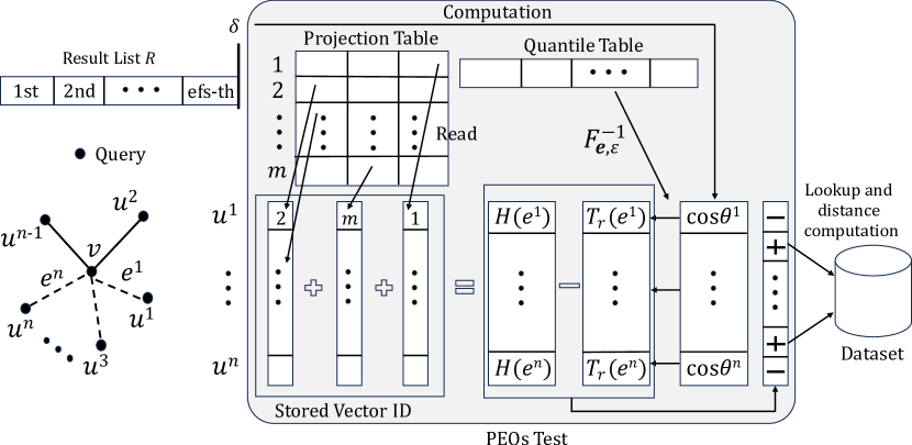
Figure 1: Illustration of the PEOs test. There are $n$ neighbors of $v$. $\theta^{1},\ldots,\theta^{n}$ denote the angles between $\bm{e}^{1},\ldots,\bm{e}^{n}$ and $\bm{q}$, respectively. $u^{2}$ and $u^{n-1}$ pass the test (indicated by “+”). We access their raw vectors from the dataset and compute their distances to $\bm{q}$.

5.3 Implementation of PEOs

In the PEOs test, Steps (1), (2), and (3) can be pre-computed during index construction. Since space partitioning may result in unbalanced norms in subspaces, we can optionally permute the dimensions so that the norms of all $\bm{e}_{i}$’s ($1\leq i\leq L,e\in E$) in the graph are as close to each other as possible (Appendix C.2). Such permutation does not affect the topology of the graph or the theoretical guarantee of PEOs. Steps (4), (5), and (6) are computed during the search. In practice, $H(\bm{e})$ and $T_{r}(\bm{e})$ can be computed efficiently because (i) $\bm{q}_{i}^{\prime\top}\bm{a}^{i}_{|e[i]|}$ and $\bm{q}^{\prime\top}\bm{b}_{|e[0]|}$ can be computed for $\bm{q}$ only once and stored in a projection table, and (ii) although the online-computation of $F^{-1}_{\bm{e},\epsilon}(x)$ is costly, we can build a lookup table containing the quantiles corresponding to the different values of the variance in $\mathcal{N}^{\bm{e},x}_{\min}$ since such variance is bounded. In particular, from the lookup table, we can choose a quantile slightly smaller than the true quantile by employing the monotonicity, which does not affect the correctness of the probability guarantee. An illustration of the implementation of the PEOs test is depicted in Figure 1. The pseudo-code is given in Algorithm 2.

Another optimization is the use of SIMD, where 16 edges can be processed at a time. This will significantly accelerate ANNS, because the raw vectors of neighbors are stored separately in the memory and loading them into CPU is costly.

Input : query $\bm{q}$, edge $e=(v,u)$, threshold $r$, projected vectors $\{\,\bm{a}^{i}_{j}\,\}$ and $\{\,\bm{b}_{j}\,\}$ ($1\leq i\leq L$, $1\leq j\leq m$), quantile table $Q$

Output : whether $u$ passes the routing test

1 Compute $A_{r}(\bm{e})$;

2 if $A_{r}(\bm{e})\geq 1$ then return (false);

3 if $A_{r}(\bm{e})\leq 0$ then return (true);

4 Normalize $\bm{q}$ to $\bm{q}^{\prime}$;

Build a projection table $T_{I}$ for all $\bm{q}_{i}^{\prime\top}\bm{a}^{i}_{j}$ and $\bm{q}^{\prime\top}\bm{b}_{j}$ ;

  /* only once and used throughout the search */

5 Compute $H(\bm{e})$ with $T_{I}$;

6 Compute $T_{r}(\bm{e})$ with $Q$;

7 if $H(\bm{e})\geq T_{r}(\bm{e})$ then  return (true) ;

8 else  return (false) ;

Algorithm 2 PEOs Test

6 Analysis of PEOs

6.1 Probability Guarantee of PEOs

To analyze PEOs, we assume $\|\bm{e}\|=\|\bm{q}\|=1$ and let $\theta$ denote the angle between them. By the independence of projected vectors in different subspaces and the result in Lemma 4.2, we have $H_{1}(\bm{e})\sim\mathcal{N}^{\theta}_{\bm{e},\bm{q}}$, where $\mathcal{N}^{\theta}_{\bm{e},\bm{q}}$ is defined as follows:

$$\mathcal{N}^{\theta}_{\bm{e},\bm{q}}=\mathcal{N}(\eta\sum\limits_{i}\|\bm{q}_{i}\|\cos\theta_{i},1-\sum\limits_{i}\|\bm{q}_{i}\|^{2}\cos^{2}\theta_{i})$$ (13)

where $\eta=\sqrt{2\ln m}$ and $\theta_{i}$ denotes the angle between $\bm{e}_{i}$ and $\bm{q}_{i}$. Next, we analyze the relationship between $\theta$ and $\mathcal{N}^{\theta}_{\bm{e},\bm{q}}$. To this end, we introduce the following definition.

Definition 6.1.

We define two partial orders $\prec$ and $\preceq$ such that, for two normal distributions $\mathcal{N}(\mu_{1},\sigma_{1}^{2})$ and $\mathcal{N}(\mu_{2},\sigma_{2}^{2})$, $\mathcal{N}(\mu_{1},\sigma_{1}^{2})\prec\mathcal{N}(\mu_{2},\sigma_{2}^{2})$ iff. $\mu_{1}\leq\mu_{2}$ and $\sigma_{1}^{2}\geq\sigma_{2}^{2}$, and $\mathcal{N}(\mu_{1},\sigma_{1}^{2})\preceq\mathcal{N}(\mu_{2},\sigma_{2}^{2})$ iff. $\mu_{1}=\mu_{2}$ and $\sigma_{1}^{2}\geq\sigma_{2}^{2}$.

With the notations defined above, we want to find an appropriate normal distribution $\mathcal{\tilde{N}}^{\theta}_{\bm{e},\bm{q}}$ such that $\mathcal{\tilde{N}}^{\theta}_{\bm{e},\bm{q}}\prec\mathcal{N}^{\theta}_{\bm{e},\bm{q}}$ ($\mathcal{\tilde{N}}^{\theta}_{\bm{e},\bm{q}}\preceq\mathcal{N}^{\theta}_{\bm{e},\bm{q}}$ is more favorable) for all adequate pairs $(\bm{e},\bm{q})$’s. We define $\mathcal{\tilde{N}}^{\theta}_{\bm{e},\bm{q}}$ as follows, where $e_{\min}=\min_{1\leq i\leq L}{\|\bm{e}_{i}\|}$ and $e_{\max}=\max_{1\leq i\leq L}{\|\bm{e}_{i}\|}$:

$$\mathcal{\tilde{N}}^{\theta}_{\bm{e},\bm{q}}=\mathcal{N}(\frac{{(\cos\theta+(e_{\min}-e_{\max})\sum\limits_{i}{\|\bm{q}_{i}\|}})\eta}{e_{\max}},1-\cos^{2}\theta).$$ (14)

Then, we have the following lemma.

Lemma 6.2.

$\mathcal{\tilde{N}}^{\theta}_{\bm{e},\bm{q}}\prec\mathcal{N}^{\theta}_{\bm{e},\bm{q}}$. When $\|\bm{e}_{1}\|=\cdots=\|\bm{e}_{L}\|$, $\mathcal{\tilde{N}}^{\theta}_{\bm{e},\bm{q}}=\mathcal{N}(\cos\theta\sqrt{2L\ln m},1-\cos^{2}\theta)\preceq\mathcal{N}^{\theta}_{\bm{e},\bm{q}}$.

From Lemma 6.2, we can see that, for the case that $e_{\max}-e_{\min}$ is large, we can only get a loose lower bound of $\mathbb{E}[\mathcal{N}^{\theta}_{\bm{e},\bm{q}}]$ due to the impact of unknown $\theta_{i}$’s (although it is possible to get a strict lower bound by solving a linear programming problem, the computation is too costly for a fast test), while the estimation of $\mathbb{E}[\mathcal{N}^{\theta}_{\bm{e},\bm{q}}]$ is always accurate when $\|\bm{e}_{1}\|=\cdots=\|\bm{e}_{L}\|$ holds. This explains why we decompose vector $\bm{e}$ into $\bm{e}_{reg}$ and $\bm{e}_{res}$ and deal with them in a separate way. Then, we have the following theorem for the probability guarantee of PEOs.

Theorem 6.3.

(1) (Probabilistic Guarantee) Suppose that $m$ is sufficiently large. The PEOs test is $(\delta,1-\epsilon)$-routing.

(2) (False Positives) Consider a neighbor $u$ whose distance to $\bm{q}$ is at least $\delta$. If $\cos\theta\leq\tilde{F}^{-1}_{\tilde{\theta}}(\epsilon)$ ($\epsilon\leq 0.5$), where $\cos\tilde{\theta}=A_{r}(\bm{e})$ and $\tilde{F}_{\theta}$ is the CDF of distribution $\mathcal{N}^{\bm{e},\cos\theta}_{\min}/\sqrt{2L\ln m}$. Then the probability that $u$ passes PEOs test is at most $1-\tilde{F}_{\theta}(\tilde{F}^{-1}_{\tilde{\theta}}(\epsilon))$.

(3) (Variance of Estimation and Comparison to RCEOs) Suppose that $H(\bm{e})/\sqrt{2L\ln m}\sim\mathcal{N}_{H}$, where $\mathcal{N}_{H}$ is an unknown normal distribution, and let $\mathcal{N}^{\theta}_{opt}=\mathcal{N}(\cos\theta,\sin^{2}\theta/(2L\ln m))$. When $w_{res}\leq 1/(L+1)$,

$$-\frac{L+2}{L(L+1)^{2}\ln m}\leq{\rm{Var}}[\mathcal{N}_{H}]-{\rm{Var}}[\mathcal{N}^{\theta}_{opt}]\leq\frac{1}{(L+1)^{2}\ln m}$$ (15)

where $\theta$ is the (unknown) angle between $\bm{e}$ and $\bm{q}$.

Remarks. (1) The first statement of Theorem 6.3 guarantees that promising neighbors can be explored with a high confidence.

(2) The second statement shows that the routing efficiency is determined by the variance of $\mathcal{N}^{\bm{e},\cos\theta}_{\min}/\sqrt{2L\ln m}$. Such variance is expected to be as small as possible since a smaller variance leads to a smaller probability of a false positive.

(3) It is easy to see that, for RCEOs with $m^{L}$ projected vectors, the distribution associated with $\cos\theta$ is $\mathcal{N}^{\theta}_{opt}$. For a comparison, we use $\mathcal{N}_{H}$ to denote the distribution of $H(\bm{e})/\sqrt{2L\ln m}$. Clearly, $\mathbb{E}[\mathcal{N}_{H}]=\mathbb{E}[\mathcal{N}^{\theta}_{opt}]$. On the other hand, the third statement shows that, if $w_{res}$ is a small value, the variances of such two distributions are very close. In this situation, the effect of PEOs is close to that of RCEOs with $m^{L}$ projected vectors, which explains why PEOs can perform much better than RCEOs empirically.

6.2 Impact of $L$

Based on the second and the third statements in Theorem 6.3, $w_{reg}$ and $w_{res}$ are critical values which control the routing efficiency. First, we want to show that $w_{reg}$ is generally close to 1. To this end, we calculate $\mathbb{E}[w_{reg}]$ under the assumption that vector $\bm{e}$ obeys an isotropic distribution. Because prevalent graph indexes (e.g., HNSW) diversify the selected edges in the indexing phase, such assumption is not very strong for the real datasets. Besides, we can permute the dimensions (Section 5.3) to make $\bm{e}$ follow an isotropic distribution. Let $\bar{w}_{reg}(L,d)$ denote $\mathbb{E}_{\bm{e}\sim U(\mathbb{S}^{d-1})}[w_{reg}]$ ($\bar{w}_{reg}(L,d)$ means that $w_{reg}$ is affected by $L$ and $d$). Then, we have the following lemma ($d^{\prime}>3$).

Lemma 6.4.

Given $L$, $d^{\prime}$, and $d^{\prime}=d/L$,

$$\bar{w}_{reg}(L,d)\geq\frac{(d^{\prime}-1)\sqrt{2Ld-3L}}{(d-1)\sqrt{2d^{\prime}+2\sqrt{3}-6}}.$$ (16)

As an example, $\bar{w}_{reg}(L,d)\geq 0.978$, when $d=128$ and $L=8$. For other reasonable choice of $L$ w.r.t. $d$, we can also obtain a $\bar{w}_{reg}(L,d)$ close to 1. Next, we analyze the relationship between $L$ and $w_{res}$ more accurately. To this end, we consider the distribution $\mathcal{N}^{\bm{e},\cos\theta}_{\min}/\sqrt{2L\ln m}$. Its expected value is $\cos\theta$ and its variance, which is expected to be as small as possible, as shown in Theorem 6.3, is of great interest to us. For its variance, we particularly focus on the remaining part $J_{rel}$ by removing the part regrading $\cos\theta$, which is a value close to 0 for most of $\bm{e}$’s. Specifically, $J_{rel}$ is defined as follows:

$$J_{rel}(L)=\frac{1+(L-1)\mathbb{E}[w_{res}^{2}(L,d)]}{L}.$$ (17)

On the other hand, for $\mathcal{N}^{\theta}_{opt}$, we have $J_{opt}(L)=1/L$, which corresponds to RCEOs with $m^{L}$ projected vectors. Due to the effect of $w_{res}$, there is a difference between $J_{opt}(L)$ and $J_{rel}(L)$. Thus, an appropriate value of $L$ should satisfies the following two requirements:

(1) (Major) $J_{rel}(L)$ should be as small as possible.

(2) (Minor) $w_{res}$ is close to $1/(L+1)$.

Here, the first requirement is to improve the routing efficiency of PEOs, which is more important, and the second one is to measure the deviation in the condition in the third statement (Theorem 6.3). In Figure 3, under the assumption of isotropic distribution, we plot the curves of $J_{rel}(L)$, $J_{opt}(L)$ and $\Delta=|w_{res}-[1/(L+1)]|$, for $d=128$, $384$ and $960$, respectively. It can be seen that (1) $w_{res}$ increases as $L$ grows, which means that $L$ should not be overlarge because $J_{rel}(L^{\prime})>J_{rel}(L)$ may occur when $L^{\prime}>L$, and (2) due to the closeness of $J_{opt}$ and $J_{rel}$, the effect of PEOs is very close to that of RCEOs with $m^{L}$ projected vectors when $L$ is small (e.g. $L\leq 8$). Based on the analysis above, we set $L$ to 8, 15, 16 for these three dimensions. By varying the value of $L$, the performance of PEOs on the real datasets with these dimensions is consistent with our analysis, which will be elaborated in Section 7.3.

6.3 Computational Cost

As for the time cost of PEOs, for $H(\bm{e})$, we need at most two multiplications, $L+1$ additions and $L+1$ reads to get $H(\bm{e})$. For $T_{r}(\bm{e})$, we need one addition, one read, two subtractions and two divisions because all the inner products and $F^{-1}_{\bm{e},\epsilon}(\cdot)$ can be obtained directly using the pre-computed tables. Empirically, the number of exact distance computation can be reduced by 70% – 80% by equipping graph-based ANNS with PEOs (Section 7.6).

As for the space cost of PEOs, for every edge, we need $L+1$ bytes for vector IDs, three bytes for weights, and two bytes or four bytes for $\|\bm{u}\|^{2}/2$ and $\|\bm{e}\|$, where the scalar quantization is used here. Such space cost is affordable for 10M-scale and smaller datasets on a single PC (Section 7.7). For 100M-scale and larger datasets, we can slightly sacrifice efficiency to significantly reduce space consumption (Section 7.8).

7 Experiments

All the experiments were performed on a PC with Intel(R) Xeon(R) Gold 6258R CPU @ 2.70GHz. All the compared methods were implemented in C++, with 64 threads for indexing and a single CPU for searching, following the standard setup in ANN-Benchmarks [6].

Table 1: Data statistics.

Dataset	Size ($|\mathcal{O}|$)	Dim. ($d$)	Type	Metric
GloVe200	1,183,514	200	Text	angular
GloVe300	2,196,017	300	Text	$\ell_{2}$
DEEP10M	9,990,000	96	Image	angular
SIFT10M	10,000,000	128	Image	$\ell_{2}$
Tiny5M	5,000,000	384	Image	$\ell_{2}$
GIST	1,000,000	960	Image	$\ell_{2}$

7.1 Datasets and Methods

We used six million-scale datasets. Their statistics can be found in Table 1. Although PEOs can be used for any graph index for ANNS, we implemented PEOs on HNSW because (1) HNSW is the most widely used state-of-the-art graph index, available in many ANNS tools, and (2) the update of HNSW is much easier than other graph indexes. Besides, a comprehensive evaluation [33] shows that no graph indexes can always outperform others in ANNS.

Besides PEOs, we select five competitors: (vanilla) HNSW, NSSG [13], Glass [35], FINGER [8], and RCEOs. The reasons for the selection are: (1) NSSG is another efficient graph index, proposed to improve the performance of NSG [14], (2) Glass is one the most competitive open-source ANNS implementations, (3) FINGER is a SOTA routing technique and also works on HNSW and it has been shown to outperform SimHash+HNSW (a baseline in Section 4.1), and (4) RCEOs is a baseline probabilistic routing algorithm.

We use the following parameter setup for the competitors:

(1) HNSW: $M=32$, $efc=2000$ for the two GloVe datasets and $efc=1000$ for the other datasets. We also used this setting for the HNSW index of FINGER, RCEOs and PEOs.

(2) NSSG: ($L$, $R$, $C$) was set to (100, 50, 60) on SIFT10M, (500, 70, 60) on GIST, and (500, 60, 60) on the other datasets, The parameter $K$ in the prepared KNN-graph was set to 400.

(3) Glass: For DEEP10M, we used Glass (+HNSW) since Glass (+NSG) failed to finish the index construction. For the other datasets, we used Glass (+NSG) since it worked better than Glass (+HNSW) especially for high recall rates. $R$ was set to 32, $L$ was set to an experimentally optimal value in $[200,2000]$.

(4) FINGER (+HNSW): All parameters were set to the recommended values in its source code. In particular, the dimension of the subspace was set to 64.

(5) RCEOs (+HNSW): The only difference with PEOs is $L=1$ in RCEOs.

(6) PEOs (+HNSW): Based on the analysis in Section 6.2, $L$ was set to 8, 8, 10, 15, 16, 20 on the six datasets sorted by ascending order of dimension. $\epsilon$ was set to 0.2 and $m=128$ such that every vector ID can be encoded by one byte.

While there are many other SOTA ANNS solutions, they are not compared here because (1) the training time of learn-to-route [5] is very long on million-scale and larger datasets, (2) Adsampling [15] is only effective for the environment without SIMD optimization, (3) Falconn++ [28] and BATLearn [23] are designed for the multi-threading environment, (4) ScaNN [17] does not outperform FINGER on million-scale datasets, (5) NGTQG [20] is a vector quantization technique for graph-based ANNS orthogonal to our routing and is generally less competitive than Glass on a high recall ($\geq$ 0.5) setting [6].

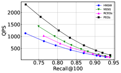
(a) GloVe200-angular, $K=100$

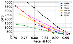
(b) GloVe300-$\ell_{2}$, $K=100$

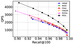
(c) DEEP10M-angular, $K=100$

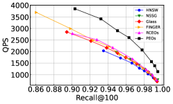
(d) SIFT10M-$\ell_{2}$, $K=100$

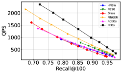
(e) Tiny5M-$\ell_{2}$, $K=100$

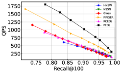
(f) GIST-$\ell_{2}$, $K=100$

Figure 2: Recall-QPS evaluation. The recalls of Glass and FINGER are lower than 30% on GloVe200 and thus not shown.

7.2 Queries Per Second (QPS) Evaluation

Figure 2 reports the recall-QPS curves of all the competitors on the six datasets. We have the following observations.

(1) On all the datasets, the winner is PEOs, trailed by FINGER in most cases. This demonstrate that our routing is effective. In particular, PEOs accelerates HNSW by 1.6 to 2.5 times and it is faster than FINGER by 1.1 to 1.4 times.

(2) The improvement of PEOs over HNSW is more significant on the datasets with more dimensions, because computing the exact distance to the query is more costly on these datasets.

(3) On GloVe200, FINGER and Glass report very low recall ($<$ 30%) recall while the improvement of PEOs over HNSW is still obvious under high recall settings. Specifically, FINGER is also based on routing, but incurs unbounded estimation errors and the errors might be very large on GloVe200, resulting in many false negatives of and rendering the graph under-explored. This result evidences the importance of the probability guarantee of routing.

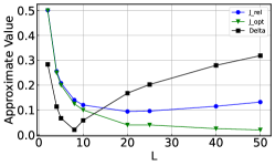
(a) Dimension: 200 (GloVe200)

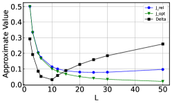
(b) Dimension: 300 (GloVe300)

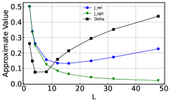
(c) Dimension: 96 (DEEP10M)

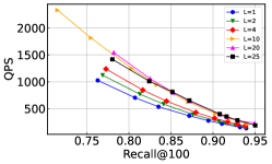
(d) GloVe200-angular, $d=200$

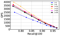
(e) GloVe300-$\ell_{2}$, $d=300$

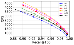
(f) DEEP10M-angular, $d=96$

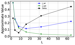
(g) Dimension: 128 (SIFT10M)

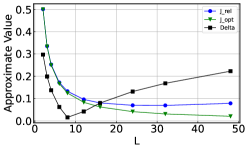
(h) Dimension: 384 (Tiny5M)

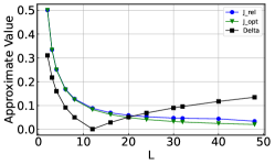
(i) Dimension: 960 (GIST)

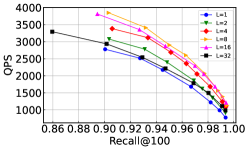
(j) SIFT10M-$\ell_{2}$, $K=100$

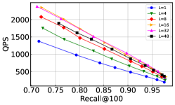
(k) Tiny5M-$\ell_{2}$, $K=100$

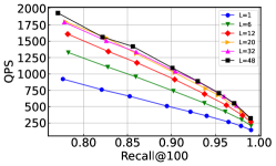
(l) GIST-$\ell_{2}$, $K=100$

Figure 3: Effect of $L$. We plot the approximate values of $J_{opt}$, $J_{rel}$, and $\Delta$ under the isotropic distribution (see Section 6.2 for interpretations) as well as the empirical performance comparison.

7.3 Effect of Space Partition Size $L$

We evaluate the effect of $L$ in PEOs and report the results in Figure 3 on the SIFT10M, Tiny5M, and GIST datasets. On each dataset, theoretical results (top) are accompanied with their empirical counterparts (bottom). The empirical results are consistent with our analysis in Section 6.2. That is, the smaller $J_{rel}$ is, the better the performance is. We also have the following observations. (1) The performance under $L>1$ is obviously better than that under $L=1$, showcasing the effectiveness of space partitioning. (2) An $L$ of 32 leads to a worse performance than an $L$ of 8 on the SIFT10M dataset, because the variance is larger when $L=32$. (3) When $L>16$ on the GIST dataset, the performance tends to be stable since the variance barely changes when $L$ exceeds 16.

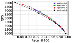
(a) DEEP100M-angular, $K=100$

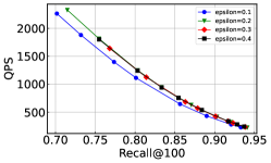
(b) GloVe200-angular, $K=100$

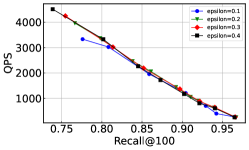
(c) GloVe300-$\ell_{2}$, $K=100$

Figure 4: Effect of $\epsilon$.

7.4 Effect of Error Bound $\epsilon$

We vary the value of $\epsilon$ and report the results in Figure 4. The performance of PEOs under $\epsilon=0.1$ is slightly worse than those under other $\epsilon$ settings. On the other hand, $\epsilon=0.2$ is consistently the best choice, leading to the best recall-QPS curve. Based on this observation, we suggest users choose $\epsilon=0.2$ to seek best performance with a guaranteed routing.

7.5 Effect of Result Number $K$

In Figure 5, we show the recall-QPS comparison under $K=10$ and $K=1$. We have the following observations.

(1) PEOs still performs the best on all the datasets, showcasing the robustness of PEOs for different values of $K$. In particular, the performance improvement of PEOs over HNSW under a small $K$ is almost consistent with that under $K=100$.

(2) The improvement of PEOs over FINGER is marginal when $K=1$. This is because the search under $K=1$ is much easier than the search under a large $K$ value. When $K$ grows, we have to accordingly increase the size of the result list, under which situation, the routing becomes harder and a more accurate estimation is important for the performance improvement.

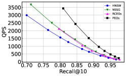
(a) GloVe200-angular, $K=10$

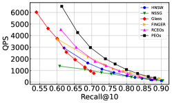
(b) GloVe300-$\ell_{2}$, $K=10$

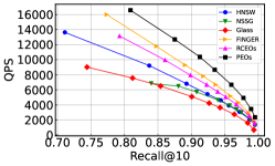
(c) DEEP10M-angular, $K=10$

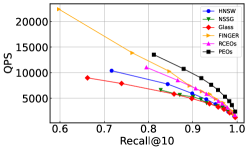
(d) SIFT10M-$\ell_{2}$, $K=10$

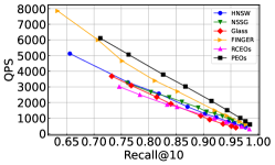
(e) Tiny5M-$\ell_{2}$, $K=10$

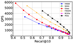
(f) GIST-$\ell_{2}$, $K=10$

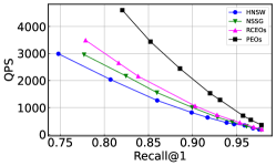
(g) GloVe200-angular, $K=1$

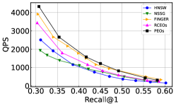
(h) GloVe300-$\ell_{2}$, $K=1$

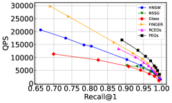
(i) DEEP10M-angular, $K=1$

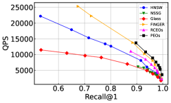
(j) SIFT10M-$\ell_{2}$, $K=1$

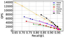
(k) Tiny5M-$\ell_{2}$, $K=1$

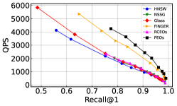
(l) GIST-$\ell_{2}$, $K=1$

Figure 5: Recall-QPS evaluation, $K=10$ and $K=1$.

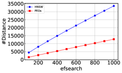
(a) GloVe200-angular, #Dist. Comput.

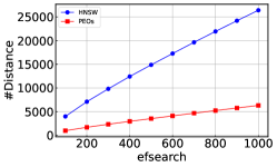
(b) GloVe300-$\ell_{2}$, #Dist. Comput.

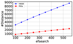
(c) DEEP10M-angular, #Dist. Comput.

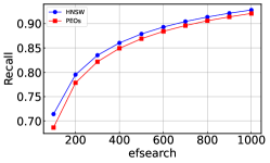
(d) GloVe200-angular, Recall

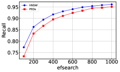
(e) GloVe300-$\ell_{2}$, Recall

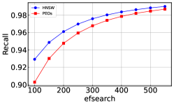
(f) DEEP10M-angular, Recall

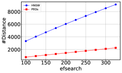
(g) SIFT10M-$\ell_{2}$, #Dist. Comput.

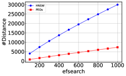
(h) Tiny5M-$\ell_{2}$, #Dist. Comput.

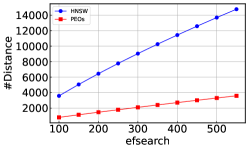
(i) GIST-$\ell_{2}$, #Dist. Comput.

(j) SIFT10M-$\ell_{2}$, Recall

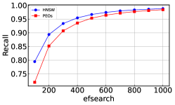
(k) Tiny5M-$\ell_{2}$, Recall

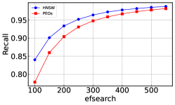
(l) GIST-$\ell_{2}$, Recall

Figure 6: Evaluation of $efs$-number of distance computations and $efs$-recall, $K=100$.

7.6 Effect of List Size $efs$

To evaluate the effectiveness of PEOs in reducing exact distance computation, we also plot the $efs$-number of distance computations and $efs$-recall curves, where $efs$ is the size of the temporary result list, adjusted to achieve a different trade-off between efficiency and accuracy. From the results in Figure 6, we have the following observations.

(1) PEOs saves around 75% exact distance computations on each dataset, and this is the main reason for the improvement on QPS. On the other hand, such improvement is not sensitive to the value of $efs$.

(2) Due to the existence of an estimation error, for the same $efs$, the recall of PEOs is smaller than that of HNSW. Nonetheless, the difference is quite small, especially for $efs>100$ (note that $efs\geq 100$ for $K=100$), thanks to the theoretical guarantee of PEOs.

(3) As $efs$ grows, the difference between the recalls of HNSW and PEOs are very small while the saved distance computation by PEOs is still large. This explains why PEOs works better for larger $efs$ values, which generally corresponds to larger $K$.

Table 2: Index size and indexing time.

Dataset	Index Size (GB)			Indexing Time (s)
	HNSW	HNSW+FINGER	HNSW+PEOs	HNSW	HNSW+FINGER	HNSW+PEOS
GloVe200	1.19	3.89 (+2.27x)	2.27 (+0.91x)	737	463+38	794+33
GloVe300	3.02	8.04 (+1.66x)	3.70 (+0.23x)	1310	1408+178	1346+24
DEEP10M	6.14	31.15 (+4.07x)	12.13 (+0.98x)	1245	1103+849	1296+208
SIFT10M	7.34	31.44 (+3.28x)	14.39 (+0.96x)	1490	1308+1025	1536+204
Tiny5M	8.44	20.49 (+1.43x)	12.89 (+0.53x)	2738	2959+1220	2880+158
GIST	3.83	6.12 (+0.60x)	4.64 (+0.21x)	738	790+706	793+40

7.7 Indexing Performance

Since the construction time of a graph index highly depends on the parameter $efc$ and PEOs does not rely on the underlying graph, we focus on the indexing time of PEOs itself. From the result in Table 2, we can see that the time of indexing for PEOs is much shorter than the time of graph construction. On the other hand, FINGER requires more indexing time because it needs to additionally construct a subspace for each node.

As for the index size, we can see that, the size of HNSW+PEOs is 1.2x – 2.0x larger than that of HNSW. On the two datasets with lower dimensions, the additional space overheads are more obvious. Meanwhile, FINGER requires more space cost than PEOs due to storing the information of generated subspaces. Next, we will give a detailed discussion on coping with the scalability issue.

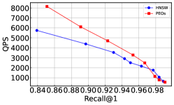
(a) DEEP100M-angular, $K=1$

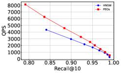
(b) DEEP100M-angular, $K=10$

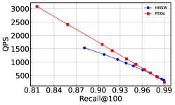
(c) DEEP100M-angular, $K=100$

Figure 7: Recall-QPS evaluation on DEEP100M. $L=2$ for PEOs.

Table 3: Index size and indexing time on DEEP100M.

Method	Index Size (GB)	Indexing Time (s)
HNSW	66.0	8877
HNSW+PEOs	67.9 (+0.029x)	5832+622

7.8 Scalability

We discuss how to tackle the scalability issue of PEOs on datasets larger than the million scale. Generally, there are the following three ways to reduce the space cost: (1) decreasing $M$, (2) decreasing $L$, and (3) using only one byte for scalar quantization. In fact, when $L\leq 4$, we know that $w_{res}$ is generally very small, which means that we can set $w_{reg}$ to 1 and $w_{res}$ to 0 for every $\bm{e}$. In this case, for each neighbor $u$, we only need $L$ bytes ($2\leq L\leq 4$) for sub-vector IDs, one byte for the norm of $\bm{u}$ and one byte for the norm of $\bm{e}$. Although such setting is not the optimal one for the search performance, it can significantly reduce additional space cost empirically, as shown below.

Following the analysis above, we use $L=2$ and $M=16$ for PEOs on DEEP100M, with 100M vectors, 96 dimensions, and angular distance as metric. Here, we only compare PEOs with HNSW since the index size of FINGER is too large to be stored on our PC. From the results in Figure 7 and Table 3, we can see that, in most cases, PEOs still has a 30% performance improvement on HNSW with a 3% additional space cost. For datasets with higher dimensions, the percentage of additional space cost can be smaller.

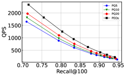
(a) GloVe200-angular, $K=100$

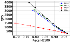
(b) GloVe300-$\ell_{2}$, $K=100$

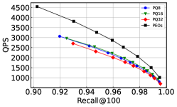
(c) DEEP10M-angular, $K=100$

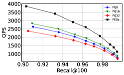
(d) SIFT10M-$\ell_{2}$, $K=100$

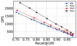
(e) Tiny5M-$\ell_{2}$, $K=100$

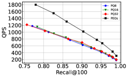
(f) GIST-$\ell_{2}$, $K=100$

Figure 8: Comparison with PQ-based routing. X in PQX denotes the number of sub-codebooks.

7.9 Comparison with Product Quantization (PQ)

We can see that PEOs has similarities with PQ [21], both partitioning the original space into orthogonal subspaces and combining the information in different subspaces. Thus, an interesting question is if the quantization techniques can be used for the acceleration of routing. First, we note that, since $|E|$ is much larger than the data size $|\mathcal{O}|$, and the local intrinsic dimensionality (LID) of $\bm{e}$’s is also very large due to the edge-selection strategy, the quantization of $\bm{e}$’s is not as effective as the quantization of raw vectors. On the other hand, apart from the probability guarantee, PEOs has the following two advantages. (1) The impact of $w_{res}$ is fully considered in PEOs while the impact of individual quantization error is hard to be measured. (2) PEOs applies a non-linear transformation, i.e., $F^{-1}_{\bm{e},\epsilon}$, to the threshold $\cos\theta$. After such transformation, as threshold $\theta$ decreases from $\pi/2$ to $0$, $T_{r}(\bm{e})$ will grow rapidly such that passing the PEOs test becomes much harder, because the possibility that a small angle $\theta$ exists between two high-dimensional vectors is very small. That is, PEOs takes the potential impact of threshold into consideration thanks to the probability guarantee. On the other hand, quantization-based techniques focus on the minimization of quantization errors and do not consider the impact of the threshold.

For an empirical evaluation, first, we need to adapt the existing quantization-based technique for routing. Specifically, we use norm-explicit product quantization [10] – which has shown competitive performance for the estimation of inner product – to quantize $\bm{e}$’s and compute the approximate inner product between $\bm{q}$ and each $\bm{e}$. Since the standard quantization generally does not consider the effect of quantization error in the search phase, to obtain better search performance, we also maintain the norm of the residual part of $\bm{e}$ after quantization, denoted by $\|\bm{e}\|_{res}$. Then we need to introduce a coefficient $c$ and write the test of quantization as follows:

$$c\|\bm{e}\|_{res}\|\bm{q}\|\geq I$$ (18)

where $I$ denotes the threshold of inner product for being added into the temporary result list, which is is computed in a similar way to $A_{r}(\bm{e})$. In practice, although we do not know the optimal value of $c$ for each dataset, we experimentally adjust it in $(0,1)$ to get a near-optimal value. By the above setting, we can compare the performances of HNSW+PEOs and HNSW+PQ. From the results in Figure 8, we have the following three observations. (1) Expect for GloVe300, PEOs obviously performs better than PQ, as analyzed in the previous discussion. (2) Due to the hardness of residual quantization, the quantization error may be quite large especially for the high-dimensional datasets, such as GIST, which makes the estimation inaccurate. (3) The impact of the number of sub-codebooks is hard to be predicted, as shown on GloVe300.

8 Conclusion

We studied the problem of probabilistic routing in graph-based ANNS, which yields a probabilistic guarantee of estimating whether the distance between a node and the query will be computed when exploring the graph index for ANNS, thereby preventing unnecessary distance computation. We considered two baseline algorithms by adapting locality-sensitive approaches to routing in graph-based ANNS, and devised PEOs, a novel approach to this problem. We proved the probabilistic guarantee of PEOs and conducted experiments on six datasets. The results showed that PEOs is effective in enhancing the performance of graph-based ANNS and consistently outperforms SOTA by 1.1 to 1.4 times.

Appendix A Proofs

A.1 Proof of Lemma 6.2

Proof.

We first consider the variance. By $\|\bm{e}\|=1$, $\|\bm{q}\|=1$ and the Cauchy-Schwarz inequality, we have

$$|\bm{e}^{\top}\bm{q}|\leq\sqrt{\sum\limits_{i}\|\bm{q}_{i}\|^{2}\cos^{2}\theta_{i}}$$ (19)

which means that ${\rm{Var}}{[\mathcal{N}^{\theta}_{\bm{e},\bm{q}}]}\leq 1-\cos^{2}{\theta}$. Next, we consider $\mathbb{E}{[\mathcal{N}^{\theta}_{\bm{e},\bm{q}}]}$. To get a lower bound of $\sum\limits_{i}\|\bm{q}_{i}\|\cos\theta_{i}$, we only need to solve the following linear programming problem, that is, to calculate $S$.

$$\begin{split}S=\min{\sum\limits_{i}{s_{i}}}\\ s.t.\quad-\|\bm{q}_{i}\|\leq s_{i}\leq\|\bm{q}_{i}\|\qquad(1\leq i\leq L)\\ \sum\limits_{i}{s_{i}\|\bm{e}_{i}\|}=\cos\theta.\end{split}$$ (20)

By replacing $s_{i}$ by $t_{i}=s_{i}+\|\bm{q}_{i}\|$, we only need to solve the following problem. Noting that all $\|\bm{q}_{i}\|$’s can be viewed as constants since $\bm{q}$ is fixed in the query phase.

$$\begin{split}S^{\prime}=\min{\sum\limits_{i}{t_{i}}}\\ s.t.\quad 0\leq t_{i}\leq 2\|\bm{q}_{i}\|\quad(1\leq i\leq L)\\ \sum\limits_{i}{t_{i}\|\bm{e}_{i}\|}=\cos\theta+\sum\limits_{i}{\|\bm{q}_{i}\|\|\bm{e}_{i}\|}.\end{split}$$ (21)

Let $\|\bm{q}_{\alpha(1)}\|\geq\|\bm{q}_{\alpha(2)}\|\cdots\geq\|\bm{q}_{\alpha(L)}\|$ and $\|\bm{e}_{\beta(1)}\|\geq\|\bm{e}_{\beta(2)}\|\cdots\geq\|\bm{e}_{\beta(L)}\|$, where $\alpha(\cdot)$ and $\beta(\cdot)$ are two permutations of $1,\cdots,L$. Let $U=\cos\theta+\sum\limits_{i}{\|\bm{q}_{i}\|\|\bm{e}_{i}\|}$. Suppose that $1\leq L^{\prime}\leq L-1$ is an integer such that the following relationship holds (noting that $U>0$ and the leftest term is set to 0 when $L^{\prime}=0$).

$$\sum\limits_{1\leq i\leq L^{\prime}}{\|\bm{q}_{\alpha(i)}\|\|\bm{e}_{\beta(i)}\|}\leq\frac{U}{2}<\sum\limits_{1\leq i\leq L^{\prime}+1}{\|\bm{q}_{\alpha(i)}\|\|\bm{e}_{\beta(i)}\|}.$$ (22)

Note that we do not need to consider the case $U/2\geq\sum\limits_{1\leq i\leq L}{\|\bm{q}_{\alpha(i)}\|\|\bm{e}_{\beta(i)}\|}$ since it does not occur for any adequate $\theta$. If it occurs, we can get the following inequality by the rearrangement inequality:

$$\cos\theta\geq\sum\limits_{i}{\|\bm{q}_{i}\|\|\bm{e}_{i}\|}.$$ (23)

In this case, we definitely know the neighbor $u$ cannot be added into the priority queue.

By (22), we can easily calculate $S^{\prime}$ in (21) as follows:

$$S^{\prime}=2\sum\limits_{1\leq i\leq L^{\prime}}{\|\bm{q}_{\alpha(i)}\|}+\frac{U-U^{\prime}}{\|\bm{e}_{\beta(L^{\prime}+1)}\|}$$ (24)

where $U^{\prime}=2\sum\limits_{1\leq i\leq L^{\prime}}{\|\bm{q}_{\alpha(i)}\|\|\bm{e}_{\beta(i)}\|}$. Then we have the following inequalities:

$$\begin{split}S^{\prime}&\geq 2\sum\limits_{1\leq i\leq L^{\prime}}{\|\bm{q}_{\alpha(i)}\|}+\frac{\cos\theta+\sum\limits_{i}{\|\bm{q}_{i}\|e_{\min}}-U^{\prime}}{e_{\max}}\\ &\geq\frac{\cos\theta+\sum\limits_{i}{\|\bm{q}_{i}\|e_{\min}}}{e_{\max}}.\end{split}$$ (25)

Thus, we have the following result on the expected value:

$$\frac{\cos\theta+(e_{\min}-e_{\max})\sum\limits_{i}{\|\bm{q}_{i}\|}}{e_{\max}}\leq S\leq\mathbb{E}{[\mathcal{N}^{\theta}_{\bm{e},\bm{q}}]}/\eta.$$ (26)

For the case $\|\bm{e}_{1}\|=\cdots=\|\bm{e}_{L}\|$, because $\sum\limits_{i}\|\bm{q}_{i}\|\cos\theta_{i}=\sqrt{L}\cos\theta$ always holds, we can prove the lemma. ∎

A.2 Proof of Theorem 6.3

Proof.

(1) In Section 5.2, from the formulation of $A_{r}({\bm{e}})$, we can see that $A_{r}({\bm{e}})$ yields a threshold of the angle between $\bm{e}$ and $\bm{q}$. Therefore, we only consider the angle between them by assuming $\|\bm{e}\|=\|\bm{q}\|=1$ to simplify the proof.

For the case when $A_{r}({\bm{e}})\geq 1$, $dist(\bm{u},\bm{q})\geq\delta$. Hence $\bm{u}$ can be safely pruned and the PEOs test returns false. For the case when $A_{r}({\bm{e}})\leq 0$, $\bm{u}$ is likely to be have a distance less than $\delta$ from $\bm{q}$, and the PEOs test always returns true. Therefore, the statement can be proved by showing that the case $0<A_{r}({\bm{e}})<1$ is $(\delta,1-\epsilon)$-routing.

By the result in Lemma 6.2, we have $w_{reg}H_{1}(\bm{e})\sim\mathcal{N}_{reg}$ and $\sqrt{L}w_{res}H_{2}(\bm{e})\sim\mathcal{N}_{res}$, where $\mathcal{N}_{reg}$ and $\mathcal{N}_{res}$ have the following properties:

$$\mathcal{N}(w_{reg}\cos\theta_{1}\sqrt{2L\ln{m}},w_{reg}^{2}(1-\cos^{2}\theta_{1}))\preceq\mathcal{N}_{reg},$$ (27)

$$\mathcal{N}_{res}=\mathcal{N}(w_{res}\cos\theta_{2}\sqrt{2L\ln{m}},w_{res}^{2}L(1-\cos^{2}\theta_{2}))$$ (28)

where $\theta_{1}$ is the angle between $\bm{e}_{reg}$ and $\bm{q}$, and $\theta_{2}$ is the angle between $\bm{e}_{res}$ and $\bm{q}$. Note that (27) holds since $e[i]=e_{reg}[i]$ ($1\leq i\leq L$). Suppose that $dist(\bm{u},\bm{q})<\delta$. Then, by the definition of $r$, the condition that $u$ can pass the PEOs test is equivalent to the following inequality:

$$\cos\theta\geq F_{\bm{e},\epsilon}(T_{r}(\bm{e}))=A_{r}(\bm{e})=\cos\tilde{\theta}>0.$$ (29)

That is, $\tilde{\theta}$ is the threshold angle. By $\|\bm{e}\|=\|\bm{q}\|=1$, we have

$$\cos\theta=\bm{e}^{\top}\bm{q}=w_{reg}\cos\theta_{1}+w_{res}\cos\theta_{2}.$$ (30)

Thus, we have the following relationship:

$$\mathcal{N}_{rel}=\mathcal{N}(\cos\theta\sqrt{2L\ln{m}},V)\preceq\mathcal{N}_{reg}+\mathcal{N}_{res}$$ (31)

where $V=w_{reg}^{2}(1-\cos^{2}\theta_{1})+w_{res}^{2}L(1-\cos^{2}\theta_{2})$. Then, we have the following claim.

Claim: if the following inequality holds:

$$V\leq w_{reg}^{2}+Lw_{res}^{2}-\frac{L\cos^{2}\theta}{L+1},$$ (32)

then, $\Pr[H(\bm{e})\geq T_{r}(\bm{e})]\geq 1-\epsilon$.

Proof of Claim: Clearly, $H(\bm{e})$ can be viewed as a random variable and $H(\bm{e})\sim\mathcal{N}_{reg}+\mathcal{N}_{res}$. Then, we have

$$\Pr[H(\bm{e})\geq Q_{\mathcal{N}_{reg}+\mathcal{N}_{res}}(\epsilon)]=1-\epsilon$$ (33)

where $Q_{\mathcal{N}}$ denotes the quantile function with respect to the normal distribution $\mathcal{N}$. By (32), we have $\mathcal{N}^{\bm{e},\cos\theta}_{\min}\prec\mathcal{N}_{rel}$. Then, it can be seen that $Q_{\mathcal{N}_{rel}}(\epsilon)\geq Q_{N^{\bm{e},\cos\theta}_{\min}}(\epsilon)$, where $\epsilon\leq 0.5$. For two normal distributions $\mathcal{N}(\mu_{1},\sigma_{1})$ and $\mathcal{N}(\mu_{2},\sigma_{2})$, when $\epsilon\leq 0.5$, $\mu_{1}\leq\mu_{2}$ and $\sigma_{1}\geq\sigma_{2}$, i.e., $\mathcal{N}(\mu_{1},\sigma_{1})\prec\mathcal{N}(\mu_{2},\sigma_{2})$, we have the following relationship:

$$\mu_{1}+\sigma_{1}\sqrt{2}erf^{-1}(2\epsilon-1)\leq\mu_{2}+\sigma_{2}\sqrt{2}erf^{-1}(2\epsilon-1).$$ (34)

That is, $Q_{\mathcal{N}(\mu_{1},\sigma_{1})}\leq Q_{\mathcal{N}(\mu_{2},\sigma_{2})}$. On the other hand, because $\mathcal{N}^{\bm{e},\cos\tilde{\theta}}_{\min}\preceq\mathcal{N}^{\bm{e},\cos\theta}_{\min}$, we have

$$\begin{split}\Pr[H(\bm{e})\geq T_{r}(e)]&=\Pr[H(\bm{e})\geq Q_{\mathcal{N}^{\bm{e},\cos\tilde{\theta}}_{\min}}(\epsilon)]\\ &\geq\Pr[H(\bm{e})\geq Q_{\mathcal{N}^{\bm{e},\cos\theta}_{\min}}(\epsilon)]\\ &\geq\Pr[H(\bm{e})\geq Q_{\mathcal{N}_{rel}}(\epsilon)]\\ &\geq\Pr[H(\bm{e})\geq Q_{\mathcal{N}_{reg}+\mathcal{N}_{res}}(\epsilon)]\\ &=1-\epsilon.\end{split}$$ (35)

Thus, the claim is proved. Note that the result in inequality (34) is used three times.

Now, the remaining work is to prove the inequality in (32). First, we introduce $W$ such that

$$W=w_{reg}^{2}\cos^{2}\theta_{1}+Lw_{res}^{2}\cos^{2}\theta_{2}.$$ (36)

To get a lower bound of $W$, we only need to solve the following linear programming problem:

$$\begin{split}W_{\min}=\min\{s_{1}^{2}+Ls_{2}^{2}\}\\ s.t.\quad s_{1}+s_{2}=\cos\theta\\ -w_{reg}\leq s_{1}\leq w_{reg}\\ -w_{res}\leq s_{2}\leq w_{res}.\end{split}$$ (37)

Because

$$\begin{split}s_{1}^{2}+Ls_{2}^{2}&=(L+1)(s_{2}-\frac{\cos\theta}{L+1})^{2}+\frac{L\cos^{2}\theta}{L+1}\\ &\geq\frac{L\cos^{2}\theta}{L+1},\end{split}$$ (38)

we prove the first statement.

(2) For the second statement, we first note that

$$\Phi_{\lambda\mathcal{N}_{1}}(Q_{\lambda\mathcal{N}_{2}}(\epsilon))=\Phi_{\mathcal{N}_{1}}(Q_{\mathcal{N}_{2}}(\epsilon))$$ (39)

where $\lambda>0$, $\mathcal{N}_{1}$ and $\mathcal{N}_{2}$ are two normal distributions, and $\Phi$ is the CDF of normal distribution. Suppose that $dist(\bm{u},\bm{q})\geq\delta$ and $H(\bm{e})/\sqrt{2L\ln m}\sim\mathcal{N}_{H}$. By the analysis for the first statement, we have

$$\mathbb{E}[\mathcal{N}_{H}]=\cos\theta.$$ (40)

$${\rm{Var}}[\mathcal{N}_{H}]\leq\frac{w_{reg}^{2}+Lw_{res}^{2}}{2L\ln m}-\frac{\cos^{2}\theta}{2(L+1)\ln m}.$$ (41)

Under the condition that $\cos\theta\leq\tilde{F}^{-1}_{\tilde{\theta}}(\epsilon)$, we can immediately prove the second statement by using a similar result in (34) again.

(3) For the third statement, let $\Delta^{\prime}={\rm{Var}}[\mathcal{N}_{H}]-{\rm{Var}}[\mathcal{N}^{\theta}_{opt}]$ and $\tau=2L\ln m$, On one hand, we have

$$\tau\Delta^{\prime}\leq(L-1)w^{2}_{res}+\frac{\cos^{2}\theta}{L+1}\leq\frac{2L}{(L+1)^{2}}.$$ (42)

On the other hand, we have

$$\begin{split}\tau\Delta^{\prime}&\geq(L-1)w^{2}_{res}+\frac{\cos^{2}\theta}{L+1}-(L+1)(w_{res}+\frac{\cos\theta}{L+1})^{2}\\ &\geq-2w^{2}_{res}-2w_{res}\\ &\geq-\frac{2L+4}{(L+1)^{2}}.\end{split}$$ (43)

Therefore, the third statement is proved. ∎

A.3 Proof of Lemma 6.4

Proof.

Since $\bm{e}\sim U(\mathbb{R}^{d})$, we can generate $\tilde{\bm{e}}\sim\mathcal{N}(0,I)$. It can be seen that $\tilde{\bm{e}}/\|\tilde{\bm{e}}\|\sim U(\mathbb{S}^{d-1})$. Then we have $\|\bm{e}_{1}\|^{2}\sim Y/(Y+Z)=Beta(d^{\prime}/2,(d-d^{\prime})/2)$, where $Y\sim\mathcal{X}^{2}(d^{\prime})$ and $Z\sim\mathcal{X}^{2}(d-d^{\prime})$. By the summation of expectations, we have the following result.

$$\mathbb{E}[w_{reg}(L,d)]=\mathbb{E}_{X}[\sqrt{LX}]$$ (44)

where $X\sim Beta(d^{\prime}/2,(d-d^{\prime})/2)]$. Let $\alpha=d^{\prime}/2$ and $\beta=(d-d^{\prime})/2$. Then we have

$$\begin{split}\mathbb{E}[w_{reg}(L,d)]&=\sqrt{L}\int_{0}^{1}\frac{x^{\alpha-\frac{1}{2}}(1-x)^{\beta-1}}{B(\alpha,\beta)}\,dx\\ &=\sqrt{L}\mathbb{E}_{X\sim Beta(\alpha-\frac{1}{2},\beta)}[X]\cdot\frac{B(\alpha-\frac{1}{2},\beta)}{B(\alpha,\beta)}\\ &=\sqrt{L}\cdot\frac{\alpha-\frac{1}{2}}{\alpha-\frac{1}{2}+\beta}\cdot\frac{B(\alpha-\frac{1}{2},\beta)}{B(\alpha,\beta)}\\ &=\frac{\sqrt{L}\Gamma(\frac{d^{\prime}-1}{2})\Gamma(\frac{d}{2})(d^{\prime}-1)}{\Gamma(\frac{d^{\prime}}{2})\Gamma(\frac{d-1}{2})(d-1)}\\ &\geq\frac{(d^{\prime}-1)\sqrt{2Ld-3L}}{(d-1)\sqrt{2d^{\prime}+2\sqrt{3}-6}}.\end{split}$$ (45)

We use the following Gautschi’s inequality to get the last inequality in (45).

$$\sqrt{x+\frac{1}{4}}\leq\frac{\Gamma(x+1)}{\Gamma(x+\frac{1}{2})}\leq\sqrt{x+\frac{\sqrt{3}}{2}-\frac{1}{2}}.$$ (46)

∎

Appendix B Comparison of Routing Tests

To compare the three routing tests in this paper (SimHash, RCEOs, and PEOs), we first introduce the following definition.

Definition B.1.

Let $\theta$ be the angle of $\bm{e}$ and $\bm{q}$ to be estimated, and let $X(\theta)$ and $Y(\theta)$ be two random variables regarding $\theta$, such that (1) $\mathbb{E}[X(\theta)]\in C^{1}$ and $\mathbb{E}[Y(\theta)]\in C^{1}$ are two strictly monotone functions of $\theta$, and (2) ${\rm{Var}}[X(\theta)]$ and ${\rm{Var}}[Y(\theta)]$ are continuous. Let $\gamma(\theta)=|(\mathbb{E}[X(\theta)])^{\prime}|/|(\mathbb{E}[Y(\theta)])^{\prime}|$, where $|(\mathbb{E}[Y(\theta)])^{\prime}|>0$. We say that the estimator associated with $Y$ is better than that associated with $X$ for $\theta$, if ${\rm{Var}}[X(\theta)]>{\rm{Var}}[\gamma(\theta)Y(\theta)]$.

Roughly speaking, for a given $\theta$, $Y$ is considered to be better than $X$ if the distributions associated with $X$ can distinguish the angles around $\theta$ more easily than those associated with $Y$. Based on Definition B.1, we have the following result.

Lemma B.2.

Suppose that SimHash uses $n$ hash functions and RCEOs uses $m$ projected vectors. If $m>\exp(n/[2\theta(\pi-\theta)])$, RCEOs is better than SimHash for $\theta$ ($0<\theta<\pi$).

Before the proof of Lemma B.2, to explain why we use Definition B.1 to compare the estimators associated with $X$ and $Y$, we prove the following claim.

Claim: Suppose that $0<\tilde{\theta}_{1}<\tilde{\theta}_{2}<\pi$ and $Y$ is better than $X$ for all $\theta$’s, where $\tilde{\theta}_{1}<\theta<\tilde{\theta}_{2}$. For an arbitrary $\theta_{1}$, where $\tilde{\theta}_{1}<\theta_{1}<\tilde{\theta}_{2}$, we can find a $\epsilon>0$ such that for any $\theta_{2}$, where $\theta_{1}-\epsilon\leq\theta_{2}\leq\theta_{1}+\epsilon$, ${\rm{Var}}[X(\theta_{1})]>{\rm{Var}}[\gamma Y(\theta_{1})]$ and ${\rm{Var}}[X(\theta_{2})]>{\rm{Var}}[\gamma Y(\theta_{2})]$, where $\gamma=|\mathbb{E}[X(\theta_{1})]-\mathbb{E}[X(\theta_{2})]|/|\mathbb{E}[Y(\theta_{1})]-\mathbb{E}[Y(\theta_{2})]|$.

Proof of the claim: this result can be immediately obtained by the continuity of ${\rm{Var}}[X(\theta)]$, ${\rm{Var}}[Y(\theta)]$, $\gamma(\theta)=|(\mathbb{E}[X(\theta)])^{\prime}|/|(\mathbb{E}[Y(\theta)])^{\prime}|$ and the mean value theorem.

This claim shows that, under the conditions in the claim, for two close angles $\theta_{1}$ and $\theta_{2}$, the variance associated with $Y$ is smaller than that associated with $X$ when the difference of expected values are the same (after scaling).

Proof.

By symmetry, we only need to consider the case $0<\theta\leq\pi/2$. To make the ranges of $\theta$ and $\cos\theta$ the same, we consider $2(n-\#Col)/n$ in SimHash and $f(m)\bm{q}^{\top}\bm{a}_{1}$ in RCEOs, where $\#Col$ denotes the collision number of the pair $(\bm{e},\bm{q})$ in SimHash and $f(m)=1/\sqrt{2\ln m}$. By the lemma of SimHash (Lemma 4.1), we have

$$X(\theta)=2(n-\#Col)/n\sim\frac{2}{n}\times B(n,\frac{{\theta}}{{\pi}}).$$ (47)

By the lemma of RCEOs (Lemma 4.2), we have

$$Y(\theta)=f(m)\bm{q}^{\top}\bm{a}_{1}\sim N(\cos{\theta},f^{2}(m)\sin^{2}{\theta})$$ (48)

where $X(\theta)$ and $Y(\theta)$ are two random variables depending on $\theta$. It is easy to verify that all the regularity conditions in Definition B.1 are satisfied. Since both of the ranges of $2\theta/\pi$ and $\cos{\theta}$ are $[0,1]$, and they are two monotone functions of $\theta$, it is feasible to compare them by the criterion in Definition B.1. First, it is easy to see that $\gamma(\theta)=2/(\pi sin\theta)$. On the other hand, we have

$${\rm{Var}}[X(\theta)]=4\theta(\pi-\theta)/(n\pi^{2}).$$ (49)

$${\rm{Var}}[\gamma(\theta)Y(\theta)]=2/(\pi^{2}\ln m).$$ (50)

Then, we can see that

$$m>\exp(n/[2\theta(\pi-\theta)])\Leftrightarrow\rm{Var}[X(\theta)]/\rm{Var}[\gamma(\theta)Y(\theta)]>1.$$ (51)

∎

Next, we consider PEOs (opt) and PEOs, where $w_{res}$ is assumed to be 0 in PEOs (opt). For PEOs (opt), the distribution associated with $\cos\theta$ can be approximated by $\mathcal{N}^{\theta}_{opt}$, and for PEOs, the distribution associated with $\cos\theta$ can be approximated by $\mathcal{N}^{\theta}_{act}$, which is defined as follows:

$$\mathcal{N}^{\theta}_{opt}\sim\mathcal{N}(\cos{\theta},\frac{\sin^{2}{\theta}}{2L\ln m}),$$ (52)

$$\mathcal{N}^{\theta}_{act}\sim\mathcal{N}(\cos{\theta},\frac{\sin^{2}{\theta}(w^{2}_{reg}+Lw^{2}_{res})}{2L\ln m}).$$ (53)

That is, $W$ in (36) is approximated by $(w^{2}_{reg}+Lw^{2}_{res})\cos^{2}\theta$. According to the previous analysis, we can see that, to make them outperform SimHash, $m$ and $L$ should satisfy the following requirements, where $m$ is sufficiently large.

$${\rm{\textbf{PEOs(opt):}}}\quad L\ln m>n/[2\theta(\pi-\theta)].$$ (54)

$${\rm{\textbf{PEOs:}}}\quad L\ln m>(w^{2}_{reg}+Lw^{2}_{res}))n/[2\theta(\pi-\theta)].$$ (55)

Based on the results above, we can approximately compare different tests by a concrete example. Let $d=384$ and $\theta=\pi/2$. Suppose that SimHash ($n=64$) is regarded as the baseline. For RCEOs, PEOs (opt) and PEOs, we check how many projected vectors are needed to make them outperform SimHash, as shown in Table 4. Here, $w_{res}$ is taken as the expected value under the isotropic distribution.

Table 4: Comparison of routing tests when $d=384$ and $\theta=\pi/2$. The baseline is SimHash ($n=64$). We show under which conditions, RCEOs, PEOs (opt), and PEOs can approximately outperform SimHash.

Routing Test	#Projected Vectors	$L$	Code Length (Byte)
SimHash	$n=64$	NA	8
RCEOs	$m>428957$	$L=1$	4
PEOs (opt)	$m=128$	$L>2.67$	4 (3+1)
PEOs	$m=128$	$L>2.69$	4 (3+1)

Appendix C Technical Extensions

C.1 Extension to MIPS

To support MIPS, we only need to use the following $A_{r}(\bm{e})$ to replace the one in (9):

$$A_{r}(\bm{e})=\frac{\bm{p}^{\top}\bm{q}-\bm{v}^{\top}\bm{q}}{\|\bm{q}\|\|\bm{e}\|}$$ (56)

where $\bm{p}$ denotes the element in the temporary result list having the smallest inner product with $\bm{q}$. The remaining procedure is completely same as that of $\ell_{2}$ metric.

C.2 Dimension Permutation

We describe the details of the optional dimension permutation in PEOs. Only in this section, we use $e_{j}$ to denote the $j$-th coordinate of $\bm{e}$, instead of the projection on the $j$-th subspace. We introduce the following notation.

$${\rm{Avg}}(e_{j})=\sum\limits_{e\in E}(e_{j})^{2}/|E|$$ (57)

where $E$ denotes the edge set of the graph index. For the dimension permutation in PEOs, we use the following greedy algorithm to permute the coordinates of data vectors, divided into four steps:

(1) We generate $L$ empty sets, denoted by $S_{1},S_{2},\cdots,S_{L}$, each representing a subspace.

(2) We compute ${\rm{Avg}}(e_{j})$ for every dimension $j$ and sort the dimensions in the ascending order of ${\rm{Avg}}(e_{j})$.

(3) We execute the allocation procedure by $d^{\prime}=d/L$ rounds. In the $l$-th round, for each $1\leq j\leq L$, we allocate dimension $(l-1)L+j$, to set $S_{i}$, where $S_{i}$ has the greatest $\sum\limits_{k\in S}{\rm{Avg}}(e_{k})$ among all the sets that have not been added any dimension in this round.

(4) After the allocation in Step 3, we permute the coordinates of all $\bm{e}$’s such that coordinate $e_{j}$ appears in the $i$-th sub-vector of $\bm{e}$ if $j$ is in $S_{i}$.

When dimension permutation is finished, we store the permutation, in order to permute the coordinates of the query for search.

References

- [1] A. Andoni and D. Beaglehole. Learning to hash robustly, guaranteed. In ICML, pages 599–618, 2022.
- [2] A. Andoni and P. Indyk. Near-optimal hashing algorithms for approximate nearest neighbor in high dimensions. Commun. ACM, 51(1):117–122, 2008.
- [3] A. Andoni, P. Indyk, T. Laarhoven, I. P. Razenshteyn, and L. Schmidt. Practical and optimal LSH for angular distance. In NeurIPS, pages 1225–1233, 2015.
- [4] A. Babenko and V. S. Lempitsky. Efficient indexing of billion-scale datasets of deep descriptors. In CVPR, pages 2055–2063, 2016.
- [5] D. Baranchuk, D. Persiyanov, A. Sinitsin, and A. Babenko. Learning to route in similarity graphs. In ICML, pages 475–484, 2019.
- [6] E. Bernhardsson. Ann benchmarks. https://github.com/erikbern/ann-benchmarks/, 2024.
- [7] M. Charikar. Similarity estimation techniques from rounding algorithms. In J. H. Reif, editor, STOC, pages 380–388. ACM, 2002.
- [8] P. H. Chen, W. Chang, J. Jiang, H. Yu, I. S. Dhillon, and C. Hsieh. FINGER: fast inference for graph-based approximate nearest neighbor search. In WWW, pages 3225–3235. ACM, 2023.
- [9] R. R. Curtin, P. Ram, and A. G. Gray. Fast exact max-kernel search. Statistical Analysis and Data Mining, 7(1):1–9, February–December 2014.
- [10] X. Dai, X. Yan, K. K. W. Ng, J. Liu, and J. Cheng. Norm-explicit quantization: Improving vector quantization for maximum inner product search. In AAAI, pages 51–58, 2020.
- [11] M. Datar, N. Immorlica, P. Indyk, and V. S. Mirrokni. Locality-sensitive hashing scheme based on p-stable distributions. In SoCG, pages 253–262, 2004.
- [12] W. Dong, C. Moses, and K. Li. Efficient k-nearest neighbor graph construction for generic similarity measures. In WWW, pages 577–586, 2011.
- [13] C. Fu, C. Wang, and D. Cai. High dimensional similarity search with satellite system graph: Efficiency, scalability, and unindexed query compatibility. IEEE Trans. Pattern Anal. Mach. Intell., 44(8):4139–4150, 2022.
- [14] C. Fu, C. Xiang, C. Wang, and D. Cai. Fast approximate nearest neighbor search with the navigating spreading-out graph. PVLDB, 12(5):461–474, 2019.
- [15] J. Gao and C. Long. High-dimensional approximate nearest neighbor search: with reliable and efficient distance comparison operations. Proc. ACM Manag. Data, 1(2):137:1–137:27, 2023.
- [16] T. Ge, K. He, Q. Ke, and J. Sun. Optimized product quantization. IEEE Trans. Pattern Anal. Mach. Intell, 36(4):744–755, 2014.
- [17] R. Guo, P. Sun, E. Lindgren, Q. Geng, D. Simcha, F. Chern, and S. Kumar. Accelerating large-scale inference with anisotropic vector quantization. In ICML, pages 3887–3896, 2020.
- [18] G. Gupta, T. Medini, A. Shrivastava, and A. J. Smola. BLISS: A billion scale index using iterative re-partitioning. In KDD, pages 486–495. ACM, 2022.
- [19] P. Indyk and H. Xu. Worst-case performance of popular approximate nearest neighbor search implementations: Guarantees and limitations. CoRR, abs/2310.19126, 2023.
- [20] Y. Japan. Neighborhood graph and tree for indexing high-dimensional data. https://github.com/yahoojapan/NGT, 2023.
- [21] H. Jégou, M. Douze, and C. Schmid. Product quantization for nearest neighbor search. IEEE Trans. Pattern Anal. Mach. Intell, 33(1):117–128, 2011.
- [22] Y. Lei, Q. Huang, M. Kankanhalli, and A. Tung. Sublinear time nearest neighbor search over generalized weighted space. In ICML, pages 3773–3781, 2019.
- [23] W. Li, C. Feng, D. Lian, Y. Xie, H. Liu, Y. Ge, and E. Chen. Learning balanced tree indexes for large-scale vector retrieval. In KDD, pages 1353–1362. ACM, 2023.
- [24] K. Lu, M. Kudo, C. Xiao, and Y. Ishikawa. Hvs: Hierarchical graph structure based on voronoi diagrams for solving approximate nearest neighbor search. PVLDB, 15(2):246–258, 2021.
- [25] Y. A. Malkov and D. A. Yashunin. Efficient and robust approximate nearest neighbor search using hierarchical navigable small world graphs. IEEE Trans. Pattern Anal. Mach. Intell, 42(4):824–836, 2020.
- [26] J. A. V. Muñoz, M. A. Gonçalves, Z. Dias, and R. da Silva Torres. Hierarchical clustering-based graphs for large scale approximate nearest neighbor search. Pattern Recognit., 96, 2019.
- [27] N. Pham. Simple yet efficient algorithms for maximum inner product search via extreme order statistics. In KDD, pages 1339–1347, 2021.
- [28] N. Pham and T. Liu. Falconn++: A locality-sensitive filtering approach for approximate nearest neighbor search. In NeurIPS, pages 31186–31198, 2022.
- [29] L. Prokhorenkova and A. Shekhovtsov. Graph-based nearest neighbor search: From practice to theory. In ICML, pages 7803–7813, 2020.
- [30] J. Qin, W. Wang, C. Xiao, Y. Zhang, and Y. Wang. High-dimensional similarity query processing for data science. In KDD, pages 4062–4063, 2021.
- [31] S. J. Subramanya, F. Devvrit, H. V. Simhadri, R. Krishnaswamy, and R. Kadekodi. Rand-nsg: Fast accurate billion-point nearest neighbor search on a single node. In NeurIPS, pages 13748–13758, 2019.
- [32] P. Sun, R. Guo, and S. Kumar. Automating nearest neighbor search configuration with constrained optimization. arXiv preprint arXiv:2301.01702, 2023.
- [33] M. Wang, X. Xu, Q. Yue, and Y. Wang. A comprehensive survey and experimental comparison of graph-based approximate nearest neighbor search. PVLDB, 14(11):1964–1978, 2021.
- [34] X. Xu, M. Wang, Y. Wang, and D. Ma. Two-stage routing with optimized guided search and greedy algorithm on proximity graph. Knowl. Based Syst., 229:107305, 2021.
- [35] Zilliz. Graph library for approximate similarity search. https://github.com/zilliztech/pyglass, 2023.