Unified Capacity Results for Free-Space Optical Communication Systems Over Gamma-Gamma Atmospheric Turbulence Channels

Abstract

In terrestrial free-space optical (FSO) communication systems, adaptive power control at the optical laser transmitters is crucial not only to prolong the life span of the laser sources, but more importantly to maintain robust and spectrally efficient communication through atmospheric turbulence. However, a comprehensive study of dynamic power adaptation in existing FSO systems is lacking in the literature. In this paper, we investigate FSO communication systems capable of adaptive laser power control with heterodyne detection (HD) and direct detection (DD) based receivers operating under shot-noise-limited conditions. Under these FSO systems considerations, we derive unified exact and asymptotic formulas for the capacities of Gamma-Gamma atmospheric turbulence channels with and without pointing errors; these novel closed-form capacity expressions are much simpler and provide new insights into the impact of varying turbulence conditions and pointing errors. Finally, the numerical results highlight the intricate relations of atmospheric fading, pointing error, and large-scale channel parameters in a typical terrestrial FSO channel setting, followed up by an accurate assessment of the key parameters determining the capacity performances of the aforementioned FSO systems revealing several interesting characteristics.

I Introduction

Laser-based free-space optical (FSO) communication has emerged as an appealing alternative to RF (radio-frequency) and optical fiber technologies in providing efficient backhaul connectivity in outdoor wireless networks. The key factors motivating this development are vast unregulated bandwidth, inherent security, low-cost transceivers, ease of installation, etc  [1]. In fact, interest in the applications of FSO-based wireless technology has rapidly grown in recent years to design communications for diverse scenarios such as terrestrial last-mile broadband access  [2], deep-space exploration  [3], disaster recovery, inter-satellite links, and some military applications  [4], and the picture is still evolving for 5G and 6G wireless communication networks.

Most practical FSO communication systems currently in use employ either of the following two detection schemes:
(i) Intensity modulation with direct detection (IM-DD): In intensity-modulated optical systems, the information signal is conveyed by the intensity of the transmitted laser beam, and there is effectively only one degree of freedom. At the receiver, the information is detected by direct impingement of the lightwave signal onto the front-end photodetector. Most commercially deployed FSO systems are based on IM-DD due to their simpler and low-cost transceiver design. However, the IM-DD scheme suffers from poor receiver sensitivity which, in turn, limits its deployment to short-haul terrestrial communications  [5],  [6].
(ii) Coherent heterodyne detection (HD): In coherent optical systems, information can be transmitted by simultaneous modulation of the optical carrier’s amplitude and phase components, thus having potential for two degrees of freedom. Coherent detection basically refers to the addition of a local optical signal (typically of different wavelength and hence the term ‘heterodyne’) to the incoming lightwave signal before it impinges onto the photodetector. Compared with the direct detection scheme, the coherent detection scheme has an improved receiver sensitivity which can be traded off with the deployment distance (long-haul) desired. Additionally, the coherent receiver can select a desired channel (in the electrical domain) using sharp RF filters (tuned at an intermediate frequency (IF) which typically is in the GHz range) and thus offers good selectivity. In contrast, the direct detection receiver selects a desired incoming lightwave signal using optical filters (typically wideband) and thus suffers severely from poor selectivity. For a detailed review of coherent detection-based optical receivers, see  [6].

From the deployment perspective, FSO communication systems face two main practical challenges in terrestrial scenarios despite their appealing virtues: first, FSO communication is susceptible to small-scale irradiance fluctuations caused by optical turbulence in the atmosphere and large-scale fading due to varying weather conditions. This typically leads to poor performance and in some cases imposes unrealistic link budget requirements  [8]. Second, since FSO communication is essentially line-of-sight (LOS) based on highly directional laser beams and photodetectors, the optical link between the transmitter (Tx) and the receiver (Rx) is prone to pointing errors caused by dynamic wind loads, Tx-Rx motion/vibration, thermal expansion, building sway, etc. Both these factors, in unison or individually, are capable of degrading the performance of an FSO communication system drastically. The reader may refer to  [8] for a comprehensive understanding of these fundamental issues and resulting performance limitations of the existing FSO systems for terrestrial applications.

In the optical wavelength regime (e.g., 850 nm/1550 nm), a laser beam transmitted on a terrestrial FSO link undergoes absorption, scattering, and irradiance fluctuations. Absorption and scattering are sensitive to atmospheric conditions such as rain, fog, and other obscurants, and the resulting optical wave attenuation is fairly deterministic. Turbulence, defined as random variations in the atmospheric refractive index, on the other hand induces wavefront distortion in the optical wave which in turn randomizes energy distribution within a cross-section of the beam leading to small-scale irradiance fluctuations [9], [10]. In the literature, several statistical models have been proposed for the irradiance fluctuation that have a strong basis in real FSO propagation scenarios. We mention a select few important and relevant models as follows: scintillation in weak turbulence is well modeled using log-normal distribution  [11]  [12], while the scintillation statistic in the weak-to-strong turbulence regimes is better described by Gamma-Gamma (GG) distribution  [12]  [13]. In addition to the advantage of mathematical tractability, these scintillation models show excellent statistical fit with the simulation/experimental measurements  [12]. Adjacently, the statistical modeling of the pointing error (jitter only) effect in the received irradiance has been carried out in  [14] while the pointing error case with non-zero boresight is reasonably modeled in  [15]. More recently, generalized turbulence channel models have been proposed based on double-generalized Gamma distribution  [16], Málaga ($\mathcal{M}$) distribution  [17], etc.

Similar to mobile RF channels, a typical terrestrial FSO channel offers opportunities to exploit in the form of small-scale fading fluctuations to maximize the spectral efficiency [18]. With the FSO transmitter capable of tracking the optical channel variations, the power of the optical laser beam can be adapted according to the channel conditions. Consider, for example, a naive scheme where the laser source transmits only when the instantaneous channel is good (above a threshold) might be reasonable at a low-power budget. The main objective of the paper is to present a unified treatment of terrestrial FSO communication systems with direct detection (DD) and heterodyne detection (HD) receivers from the spectral efficiency improvement perspective: dynamic optical power adaptation is applied at the laser beam source to exploit the temporal irradiance fluctuations created by the GG atmospheric turbulence and/or pointing error conditions. Our results provide interesting insights about the effect of the individual scintillation effects of turbulence and pointing error on the capacity losses/gains in these FSO systems.

There has been significant work on analyzing the capacity performance of single-link FSO systems based on IM-DD and HD detection schemes operating over generalized turbulence channels (see  [16],  [17],  [19] and references cited therein), over Log-normal and Gamma-Gamma turbulence conditions (see  [20],  [21],  [22] and references cited therein), etc. However, almost all of these research works have ignored the crucial aspect of dynamic power allocation at the optical transmitters for terrestrial FSO links. This is perhaps due to analytical difficulties in evaluating the capacity integrals involved. In  [23]  [24], Lapidoth and Moser provide capacity bounds for the (unfaded) IM-DD based FSO channel under average and/or peak power constraints imposed on the intensity of the laser beam. In particular, it is shown that the capacity bounds (both upper and lower) converge under average-power constraint at high optical powers  [23, Theorem  7  and  Proposition  8], which we will utilize later (in subsection III-C) to develop the capacity utility for the input-dependent IM-DD system model.

I-A Contribution and Organization of This Paper

The goal of this paper is to present a unified understanding of the capacity performances of existing FSO terrestrial communication systems with transmit laser power adaptation under GG atmospheric turbulence conditions. The GG atmospheric turbulence details along with the pointing error model are provided in Section II. The considered FSO system models and their relevant noise sources are explained in great detail in Section III. We list the key contributions of this paper below with respect to closely related earlier works.

• Capacity studies of many well-known fading channels typically involve integrals which are often formidable to evaluate analytically. As an alternative approach, the problem is often circumvented by employing special functions or solved by making simplifying approximations. To give a directly related example, the authors in  [21] have extensively used integral identities to express optical channel capacity (IM/DD scheme in GG turbulence) in terms of special Meijer’s G function for various laser power adaptation schemes. Although these capacity formulas are compact (Meijer’s G-based) but give little insight into questions related to the impact of fading statistics and power constraints, etc.
  Our work, in part, aims to improve upon the work of  [21] mentioned above: we first attempt to give more explicit ‘exact’ capacity formulas (unified for both IM/DD and HD schemes) for both with and without pointing error cases. This is achieved by evaluating two new integrals and the resulting identities are new to the best of our knowledge. These more explicit formulas are also amenable for further simplification in the asymptotic regimes of optical powers which are lacking in the results of  [21].

• In a related recent work  [19], Ansari et al. have developed unified capacity results for the IM/DD and HD schemes under Málaga ($\mathcal{M}$) distribution (of which GG distribution is a special case). However, optical power adaptation at the laser source (transmitter) is not explored in  [19]. For a medium/long-haul terrestrial FSO system to operate satisfactorily in dynamic atmospheric turbulence, adapting optical transmission opportunistically improves the long-term throughput efficiency (or can be traded for an improved link budget). Furthermore, it is crucial to adapt laser power efficiently to maintain low power consumption which also enhances the average life span of the laser sources  [25]. As per the authors’ best knowledge, this is a first attempt at unified exact capacity analysis (with transmit laser power control) of IM/DD and HD schemes based FSO communication systems in GG atmospheric turbulence under shot-noise-limited conditions.

• More specifically, for the GG turbulence channel with and without pointing errors, we present a unified closed-form solution in subsection IV-A for the capacities of the IM/DD and HD FSO systems employing laser power control at the optical transmitter side. Our main results in Theorems 5 and 6 are much more explicit in comparison to an equivalent result reported in [21, Eq. (23)] and hence provides a more comprehensive picture. In subsection IV-B, these results are subjected to asymptotic analysis in the extreme SNR regimes providing more concrete information on the key fading and pointing error parameters (in action) controlling the FSO systems capacity performances. To focus more on the implications of these results, the proofs of the exact and asymptotic results are relegated to Sections V and VI respectively. Several quantitative insights are derived from the numerical results presented in subsection IV-C.

• The unified analysis presented in this work should serve as a baseline for further rigorous comparison of more practical HD and IM/DD detection-based FSO communication systems with transmit power control mechanisms operating under realistic atmospheric conditions. While the IM/DD FSO scheme is the simplest (in hardware) and widely used, this study confirms quantitatively the superiority of the HD FSO systems in delivering very high throughputs albeit with a more complex engineering design. The presented results should help the system designer navigate the tradeoffs between the two FSO system choices under constraints of cost and performance.

Finally, concluding remarks are provided in Section VII.

I-B Mathematical Notations

We use the following notations throughout the paper: the probability density function (PDF) of a random variable $X$ is denoted by $f_{X}(\cdot)$ and $\mathbb{E}[\cdot]$ denotes the expected value of the enclosed. The real, non-negative real and complex number sets are denoted by $\mathbb{R}$, $\mathbb{R}^{+}$ and $\mathbb{C}$, respectively. $\Gamma(\cdot)$ is the Gamma function  [26, Eq.  (8.310.1)], $K_{v}(\cdot)$ is the modified Bessel function of the second kind and order $v$  [26, Eq.  (8.494.1)], $G_{p,q}^{m,n}(\cdot)$ is the Meijer-G function  [26, Eq.  (9.301)], $\psi(\cdot)$ is the Digamma function  [26, Eq.  (8.360.1)], and $\text{erf}(\cdot)$ denotes the standard error function  [26, Eq.  (8.250.1)]. All logarithms in this paper are natural logarithms.

II Optical Fading Channel

The (overall) intensity fluctuation $I$ experienced by the transmitted laser beam due to atmospheric turbulence and pointing error is modeled as

$$I\,=\,I_{l}I_{\mathrm{a}}I_{\mathrm{p}}$$ (1)

where $I_{l}$ is the path loss component determined by the exponential Beers-Lambert Law for a given link length and weather conditions [27], $I_{\mathrm{a}}$ is the turbulence-induced scintillation, and $I_{\mathrm{p}}$ is the pointing-error induced fluctuation.

In this work, we consider that the large-scale component $I_{l}$ is deterministic and fixed under the assumption of a fixed-length optical link with homogeneous weather conditions at all times. We will consider $I_{l}=1$ for simplicity and instead focus on the small-scale components $I_{\mathrm{a}}$ and $I_{\mathrm{p}}$ which are independent and randomly time-varying in nature. In the following subsections, we describe the statistical models adopted for these fading constituents. These models are quite reasonable for medium to long-distance terrestrial FSO links.

II-A Gamma$-$Gamma Atmospheric Turbulence

To cover a wide range of atmospheric turbulence from the weak-to-strong regime, the statistics of the intensity fluctuation $I_{\mathrm{a}}$ is well modeled using the Gamma-Gamma (GG) distribution as follows  [12]:

$$f_{I_{\mathrm{a}}}(I_{\mathrm{a}})=\frac{2(ab)^{(a+b)/2}}{\Gamma(a)\Gamma(b)}I_{\mathrm{a}}^{{(a+b)/2-1}}K_{a-b}\left(2\sqrt{abI_{\mathrm{a}}}\right);\ I_{\mathrm{a}}>0.$$ (2)

Ideally, the light from a laser source is understood to have a Gaussian beam profile, with its intensity distribution being a circularly symmetric Gaussian function across the beam cross-section and centered about the beam axis  [28, Ch. 3]. Close to its center, the Gaussian beam is approximated by a plane wave, while the wave resembles a spherical wave when it is far from the beam waist yet inside the beam waist radius  [28]. Considering optical radiation at the (far away) receiver to be a plane wave, the GG distribution parameters $a$ and $b$ can be directly related to atmospheric conditions through the following expressions [12]:

$$a\, =\,{\left({\exp\left[{\frac{{0.49\sigma_{\mathrm{R}}^{2}}}{{{{\Bigl{(}{1+1.11\sigma_{\mathrm{R}}^{12/5}}\Bigr{)}}^{7/6}}}}}\right]-1}\right)^{-1}},$$ (3)

$$b\, =\,{\left({\exp\left[{\frac{{0.51\sigma_{\mathrm{R}}^{2}}}{{{{\Bigl{(}{1+0.69\sigma_{\mathrm{R}}^{12/5}}\Bigr{)}}^{5/6}}}}}\right]-1}\right)^{-1}}.$$ (4)

In this respect, $\sigma_{\mathrm{R}}^{2}=1.23\,C_{\mathrm{n}}^{2}k_{\mathrm{w}}^{7/6}{L^{11/6}}$ denotes the Rytov variance determining the strength of the atmospheric turbulence, $k_{\mathrm{w}}=2\pi/{\lambda_{\mathrm{w}}}$ is the optical wave number, where ${\lambda_{\mathrm{w}}}$ is the wavelength, $L$ is the propagation distance, and $C_{\mathrm{n}}^{2}$ is the altitude-dependent refractive-index structure parameter. At a given altitude, $C_{\mathrm{n}}^{2}$ can be practically assumed to be constant for the line-of-sight propagation on horizontal paths [29, Ch. 2]).

II-B Pointing Error

Pointing error is basically a mispointing of the laser beam with respect to the optical receiver that arises from i) boresight and ii) jitter: boresight is the fixed displacement between the received beam centroid and the detection receiver center whereas jitter is the random temporal displacement originating due to building sway, wind motion, Tx/Rx vibrations, etc.

In this work, we consider FSO communication between fixed platforms in terrestrial environments where it is reasonable to assume that the boresight problem can be made negligible by either careful system deployment or using a fast-tracking transmitter whereas the random jitter issue persists [10]. A Gaussian beam is typically defined in terms of its physical attributes such as intensity, beam divergence, beam waist, etc. Specifically, the waist $w_{\mathrm{L}}$ of a Gaussian beam is determined from the radial distance away from the axis where the irradiance drops to $1/e^{2}$ of the maximum intensity  [28]. The transmitted laser beam, upon propagating a distance $L$, is incident on the receiving photodetector with an aperture radius $r_{\mathrm{A}}$. The attenuation of the received optical beam due to turbulence-induced beam spread with pointing error (the misalignment is described by radial displacement $r$ in the receiver plane between the centers of the beam footprint and the detector aperture) is given by $\displaystyle I_{\mathrm{p}}(r;L)\approx A_{0}\exp(-2r^{2}/w_{\mathrm{L_{eq}}}^{2})$ where $w_{\mathrm{L_{eq}}}^{2}=w_{\mathrm{L}}^{2}\sqrt{\pi}\,\text{erf}(v)/(2v\exp(-v^{2}))$ is the (squared) equivalent beam width with $v=\sqrt{\pi}r_{\mathrm{A}}/\sqrt{2}w_{\mathrm{L}}$, and

$$A_{0}=[\mathrm{erf}(v)]^{2}$$ (5)

is the fraction of the collected power at $r=0$ (i.e., no pointing error but only geometrical loss) [30]. Note that $0\leqslant A_{0}\leqslant 1$. For a coherent collimated beam, the beam radius $w_{\mathrm{L}}$ at the distance $L$ is related to the beam waist $w_{0}$ at the exit aperture of the optical transmitter by $\displaystyle w_{\mathrm{L}}=w_{0}(1+\epsilon(\lambda_{\mathrm{w}}L/\pi w_{0}^{2}))^{1/2}$ where $\epsilon=(1+2w_{0}^{2}/\rho_{0}^{2}(L))$ is the global coherence parameter and $\rho_{0}(L)=(1.46C_{\mathrm{n}}^{2}k_{\mathrm{w}}^{2}L)^{-3/5}$ is the coherence length of a plane wave propagating in turbulence  [31]. Farid and Hranilovic [30] derived the PDF of the irradiance component $I_{\mathrm{p}}$ under the i.i.d. zero-mean Gaussian distribution assumptions for both the horizontal and vertical sways at the receiver (i.e., zero boresight and identical jitters) and is given by

$$\phantom{xxxxxxxxxx}f_{I_{\mathrm{p}}}(I_{\mathrm{p}})\,=\,\frac{\xi^{2}}{A_{0}^{\xi^{2}}}I_{\mathrm{p}}^{\xi^{2}-1};\ \ \ 0\leqslant I_{\mathrm{p}}\leqslant A_{0}$$ (6)

where the parameter $\xi\triangleq{w_{\mathrm{L_{eq}}}}/{2\sigma_{\mathrm{e}}}$ is the ratio of the received equivalent beam waist $w_{\mathrm{L_{eq}}}$ and the standard deviation of the pointing error displacement (jitter) at the detection receiver. It is important to keep in mind that the probability model (6) for pointing error is reasonable when $w_{L}/r_{A}\gg 1$ (see [30, 32]) and further that the effects of $\xi$ and $A_{0}$ parameters are independent.

II-C Gamma–Gamma Turbulence with Pointing Error

The PDF of the instantaneous composite irradiance $I$ in terms of the independent constituents, namely the atmospheric turbulence $I_{\mathrm{a}}$ and the pointing error $I_{\mathrm{p}}$, is obtained as follows:

$$f_{I}(I)\,=\,\int f_{I|I_{\mathrm{a}}}(I|I_{\mathrm{a}})f_{I_{\mathrm{a}}}(I_{\mathrm{a}})dI_{\mathrm{a}}$$ (7)

where, $f_{I|I_{\mathrm{a}}}(I|I_{\mathrm{a}})$ is the conditional PDF given $I_{\mathrm{a}}$, and is expressed as

$$f_{I|I_{\mathrm{a}}}(I|I_{\mathrm{a}})=\frac{\xi^{2}}{A_{0}^{\xi^{2}}I_{\mathrm{a}}}\left(\frac{I}{I_{\mathrm{a}}}\right)^{\xi^{2}-1};\ 0\leqslant I\leqslant A_{0}I_{\mathrm{a}}.$$ (8)

Substituting (8) and (2) in (7), we get

$$f_{I}(I)\,= \,\frac{2\xi^{2}(ab)^{(a+b)/2}}{\left(A_{0}I_{1}\right)^{\xi^{2}}\Gamma(a)\Gamma(b)}I^{\xi^{2}-1}$$

$$\cdot\,\int_{I/A_{0}}^{\infty}I_{\mathrm{a}}^{(a+b/2)-1-\xi^{2}}K_{a-b}\left(2\sqrt{abI_{\mathrm{a}}{}}\right)dI_{\mathrm{a}}.$$ (9)

A closed-form to the integral in (II-C) is provided by using the integral identity  [26, Eq.  (6.592.4)] with  [26, Eq. (9.31.5)] as follows:

$$f_{I}(I)=\frac{ab\xi^{2}}{A_{0}\Gamma(a)\Gamma(b)}G_{1,3}^{3,0}\left(\frac{abI}{A_{0}}\,\biggr{\rvert}\begin{array}[]{c}\xi^{2}\\[1.00006pt] \xi^{2}-1,\,a-1,\,b-1\\ \end{array}\right).$$ (10)

Remark 1.

$\mathbb{E}[I_{\mathrm{a}}]=1$ for the GG distribution in (2) and $\mathbb{E}[I_{\mathrm{p}}]=A_{0}\,\xi^{2}/(1+\xi^{2})$ for the pointing error PDF in (6). Hence, the mean of the overall irradiance $I$ is given by

$$\mathbb{E}[I]\,=\,\mathbb{E}[I_{\mathrm{a}}]\,\mathbb{E}[I_{\mathrm{p}}]\,=\,A_{0}\,\xi^{2}/(1+\xi^{2}).$$

Remark 2.

It should be noted that for $A_{0}\rightarrow 1$ and $\xi\rightarrow\infty$, the composite irradiance distribution in (10) tends to the pure GG distribution in (2) as a special (extreme) case.

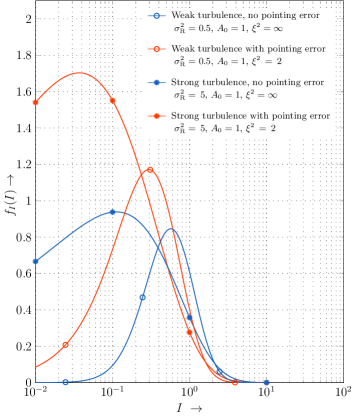
Figure 1: The probability density function of overall irradiance $I$ in the weak and strong turbulence regimes. Higher atmospheric turbulence suggests an increased probability for small channel gains and vice-versa. The presence of pointing error also leads to probability concentration at low channel gains.

As mentioned earlier, terrestrial FSO communication suffers from irradiance fluctuations due to atmospheric turbulence and/or misalignment errors. This is illustrated in Fig. 1 where the overall irradiance distribution (10) is plotted for varying levels of turbulence and pointing errors. From this figure, we can notice that although turbulence-induced fading is the principal impediment, the sensitivity of the overall irradiance distribution to pointing error also becomes particularly acute even for mild random jitter variance. A more in-depth and unified understanding of the resulting performance loss in terms of channel capacity is an important objective of this paper.

III System Model & Capacity Definition

In this section, we first provide a brief necessary background on the noise sources relevant to the FSO optical receivers (subsection III-A). We then proceed to develop the signal models for the shot-noise-limited IM/DD and HD-based receivers in subsection III-B.

III-A Receiver Noises in FSO Wireless Systems

In optical receivers, photodiodes are the most commonly used device to detect photons (or photodetection) with the objective of transforming an information-bearing optical signal into a photocurrent (electrical) signal with a one-to-one correspondence. Two fundamental sources of noise unavoidably stem out in the process of photodetection: i) the shot noise arising due to photodetection itself, and ii) the thermal noise originating post-detection in the receiver circuitry.

Remark 3.

The electrical-to-optical (E/O) conversion at the transmit side and optical-to-electrical (O/E) conversion at the receiver typically admit losses which we have ignored for simplicity. These Tx./Rx. conversion losses can be adjusted in the optical link budget similar to the path loss component.

The shot noise induced at the photodetector output is signal-dependent in the sense that its power grows linearly with the total incident optical power (say $P_{\mathrm{in}}$). Since both thermal noise and shot noise are additive in nature and are statistically independent of each other, the total (electrical) noise variance can be expressed as their summation, i.e., $\sigma_{\mathrm{Total}}^{2}=\sigma_{\mathrm{Th}}^{2}+\sigma_{\mathrm{Sh}}^{2}$, where $\sigma_{\mathrm{Th}}^{2}=\frac{4kT\Delta f}{R_{\mathrm{L}}}$ and $\sigma_{\mathrm{Sh}}^{2}=2qRP_{\mathrm{in}}\Delta f$ denote the variance of thermal noise and shot noise, respectively. Here, $k$ is the Boltzmann constant, $T$ is the absolute temperature in Kelvin, $R_{\mathrm{L}}$ is the load resistance, $\Delta f$ is the noise equivalent bandwidth of the photodetector and $q$ is the electronic charge.

As mentioned earlier, in a coherent receiver, an optical local oscillator (OLO) signal is added to the received optical signal, and then the resulting optical signal is directed towards a photodetector device. For convenience of discussion, the resultant shot noise can be further divided into two independent parts: (i) information-signal-dependent shot noise resulting from the incoming information-bearing optical signal, and (ii) OLO-dependent shot noise proportional to the OLO optical power (typically fixed). It turns out that the average power of the information-signal-dependent shot noise (of the photocurrent induced) is proportional to the product of the OLO optical power times the received optical signal power [33]. By ensuring a large fixed OLO optical power, the OLO-dependent shot noise component can be made dominant while the effects of the thermal noise and information-signal-dependent shot noise can be made relatively insignificant  [6]  [34]. This, i.e., OLO-induced-shot-noise conditions, is in fact considered to be the de facto mode of operation of an (ideal) coherent optical receiver.

In an IM/DD optical system, the intensity-modulated optical signal upon reception is fed directly to the front-end photodetector. The consequent photocurrent at the detector output has a composition as follows: photocurrent (electrical) component with a one-to-one correspondence to the intensity of the incoming optical signal, information-signal-dependent shot noise (recall that there is no OLO here), and thermal noise. Depending on the relative strengths of these two noise components, one can readily infer if the IM/DD optical receiver is operating in shot-noise-limited conditions or thermal noise dominant conditions. For example, in a power-limited system operating at the minimum required power, thermal noise typically dominates over shot noise. In IM/DD optical systems with large received optical powers (typically holds for most terrestrial FSO systems), the signal-dependent shot noise component becomes the dominant noise source while the thermal noise component can be neglected.

A short note on the statistical properties of the shot noise: when the number of received photons per symbol period (or per channel use) is insignificant (e.g., inter-satellite and ground-satellite optical communication), a Poisson model is adequate; otherwise, a Gaussian model suffices  [35]. The Gaussian approximation is adequate for most terrestrial application systems; for those interested in a rigorous proof of the Gaussian distribution of the high-intensity shot noise, refer  [35]  [36].

III-B Detection Schemes

In this subsection, we will develop received signal models in the IM/DD and synchronous HD schemes.

Let $x_{\mathrm{\scriptscriptstyle IMDD}}\in\mathbb{R}^{+}$ and $x_{\mathrm{\scriptscriptstyle HD}}\in\mathbb{C}$ denote the transmitted signals for the IM-DD and coherent HD systems respectively. In both schemes, the laser source at the transmitter side is constrained by a fixed average (optical) power per symbol constraint as $\mathbb{E}[x_{\mathrm{\scriptscriptstyle IMDD}}]\leqslant P_{\mathrm{avg}}$ and $\mathbb{E}\left[|x_{\mathrm{\scriptscriptstyle HD}}|^{2}\right]\leqslant P_{\mathrm{avg}}$. We remind the reader that the baseband (information) signal in a coherent HD scheme represents a complex optical field, whereas the baseband signal in an IM-DD scheme represents optical intensity. Hence, the optical power constraint in the IM-DD scheme and HD scheme is on the expected value of the signal $x_{\mathrm{\scriptscriptstyle IMDD}}$ and on the magnitude-squared signal component $|x_{\mathrm{\scriptscriptstyle HD}}|^{2}$ respectively. Adhering to this understanding, the received signal models for the two detection systems are developed next.

III-B1 Signal-Dependent IM-DD Channel

The baseband channel (post photodetection) in an IM/DD system is given as

$$y_{\mathrm{\scriptscriptstyle IMDD}}\,:=\,Ix_{\mathrm{\scriptscriptstyle IMDD}}\ +\,\sqrt{Ix_{\mathrm{\scriptscriptstyle IMDD}}}\,n_{\mathrm{\scriptscriptstyle S}}\,+\,z_{\mathrm{\scriptscriptstyle T}}$$ (11)

where $y_{\mathrm{\scriptscriptstyle IMDD}}$ is the received intensity, $x_{\mathrm{\scriptscriptstyle IMDD}}$ being the transmitted intensity, $I$ is the intensity fluctuation due to atmospheric turbulence and misalignment, $z_{\mathrm{\scriptscriptstyle T}}\sim\mathcal{N}(0,\sigma_{\mathrm{\scriptscriptstyle T}}^{2})$ is the signal-independent additive white Gaussian (AWGN) thermal noise, and the scaled component $\sqrt{Ix_{\mathrm{\scriptscriptstyle IMDD}}}\,n_{\mathrm{\scriptscriptstyle S}}\sim\mathcal{N}(0,Ix_{\mathrm{\scriptscriptstyle IMDD}}\sigma_{\mathrm{\scriptscriptstyle S}}^{2})$ is the signal-dependent AWGN shot noise. Here, $\,\sqrt{Ix_{\mathrm{\scriptscriptstyle IMDD}}}\,$ is the scaling term introduced to make the noise variance proportional to the intensity of the received optical signal. As mentioned earlier, the Poisson distribution approximation with a Gaussian distribution is the reason for the formation of Gaussian signal-dependent shot noise.

In this work, we consider a shot-noise-limited IM-DD receiver which is typically valid for terrestrial FSO optical operations with large received optical powers. Hence, the total noise variance of the input-dependent IM-DD system (say, $\sigma_{\mathrm{\scriptscriptstyle IMDD}}^{2}$) is dominated by $Ix_{\mathrm{\scriptscriptstyle IMDD}}\sigma_{\mathrm{\scriptscriptstyle S}}^{2}$ due to relatively negligible thermal noise component. Thus $\displaystyle\sigma_{\mathrm{\scriptscriptstyle IMDD}}^{2}\,\approx\,Ix_{\mathrm{\scriptscriptstyle IMDD}}\,\sigma_{\mathrm{\scriptscriptstyle S}}^{2}$. Correspondingly, conditioned on the intensity fluctuation coefficient $I$, the instantaneous received (electrical) SNR is defined as

$$\gamma_{\mathrm{\scriptscriptstyle IMDD}}\,:=\,{Ix_{\mathrm{\scriptscriptstyle IMDD}}}/{\sigma_{\mathrm{\scriptscriptstyle S}}^{2}}$$ (12)

III-B2 Coherent (Heterodyne) Detection

The complex baseband channel in a coherent HD system is described by

$$y_{\mathrm{\scriptscriptstyle HD}}\,:=\,hx_{\mathrm{\scriptscriptstyle HD}}\,+\,n_{\mathrm{\scriptscriptstyle HD}}\,+\,w_{\mathrm{\scriptscriptstyle T}}$$ (13)

where $h\in\ \,\mathbb{C}$ is the channel state, $x_{\mathrm{\scriptscriptstyle HD}}\ \in\ \mathbb{C}$ its input, $y_{\mathrm{\scriptscriptstyle HD}}\ \in\ \mathbb{C}$ its output, $w_{\mathrm{\scriptscriptstyle T}}\sim\mathcal{CN}(0,2\sigma_{\mathrm{\scriptscriptstyle T}}^{2})$ the complex AWGN thermal noise, and $n_{\mathrm{\scriptscriptstyle HD}}\sim\mathcal{CN}(0,\sigma^{2}_{\mathrm{\scriptscriptstyle OLO}})$ the (OLO-induced) complex AWGN shot noise. Note that $h$ represents the fluctuation in the received (complex) optical field and hence $I\,=\,|h|^{2}$ is the intensity fluctuation.

We recall that in an ideal coherent detection receiver, the OLO-induced shot noise is the only dominant noise and thus the total noise power (denoted by $\sigma^{2}_{\mathrm{\scriptscriptstyle HD}}$) can be approximated by $\sigma^{2}_{\mathrm{\scriptscriptstyle OLO}}$. That is $\displaystyle\sigma^{2}_{\mathrm{\scriptscriptstyle HD}}\,\approx\,\sigma^{2}_{\mathrm{\scriptscriptstyle OLO}}$. Conditioned on the channel coefficient $h$ representing fluctuation in the optical field, the instantaneous (electrical) SNR is defined as

$$\gamma_{\mathrm{\scriptscriptstyle HD}}\,:=\,{I\,|x_{\mathrm{\scriptscriptstyle HD}}|^{2}}/{\sigma_{\mathrm{\scriptscriptstyle OLO}}^{2}}.$$ (14)

III-C Ergodic Capacity

The transmitted signal $x_{\mathrm{\scriptscriptstyle IMDD}}$ in the IM-DD scheme, being optical intensity, is non-negative, while the HD scheme suffers from no such limitation and in fact can support two degrees of freedom. Consequently, the well-known Shannon’s AWGN channel capacity is applicable in the HD scheme but not the IM-DD systems (see  [23]).

Based on the received SNRs in (12) and (14), i.e. conditioned on intensity fluctuation coefficient $I$, the capacities of the optical channels (in nats per symbol) based on IM-DD and HD schemes satisfy

$$C_{\mathrm{\scriptscriptstyle IMDD}}\, \geq\,\tfrac{1}{2}\log\left(1+\tfrac{e}{2\pi}\gamma_{\mathrm{\scriptscriptstyle IMDD}}\right),$$ (15)

$$C_{\scriptscriptstyle\mathrm{HD}}\, =\,\,\log(1+\gamma_{\mathrm{\scriptscriptstyle HD}}).$$ (16)

The lower bound (15) on the capacity of the signal-dependent IM-DD channel is deduced from a well-known result in  [23, Theorem 7] derived for AWGN IM-DD channel under average-power constraint. More critically, the lower bound is shown to converge to the actual capacity at high received optical powers  [23, Proposition  8]. As already mentioned, we consider the IM-DD channel with high received optical powers, and hence the lower bound is in fact a very accurate estimate of the actual capacity.

Based on the above observation and the symmetry of the two FSO systems capacity formulae in (15)and (16), an interesting unification of the two channel capacity expressions (for fixed channel state) into a single one is possible by introducing a generic parameter $k$ as follows:

$$C(\lambda)\,:=\,\frac{1}{k}\log\left(1+\frac{\lambda P_{k}(\lambda)}{N_{k}}\right)$$ (17)

where $k=1,\,N_{1}\,=\,{\sigma^{2}_{\mathrm{\scriptscriptstyle OLO}}}\,,\,P_{1}(\lambda)\,:=\,|x_{\mathrm{\scriptscriptstyle HD}}|^{2}$ for the HD based scheme and for the IM-DD based scheme, we have $k=2,\,N_{2}=\sigma_{\mathrm{\scriptscriptstyle S}}^{2}\tfrac{e}{2\pi},\,P_{2}(\lambda)\,:=\,x_{\mathrm{\scriptscriptstyle IMDD}}$. Notice that $\lambda$ can be viewed as channel (intensity) gain and $P_{k}(\lambda)$ as the transmitted signal intensity. We average over the random channel gain $\lambda$ to find the overall average capacity.

We will maximize the (average) optical channel capacity by adapting the laser beam power $P_{k}(\lambda)$ optimally at the transmitter according to the stationary and ergodic time-varying channel fluctuations $\lambda$. Power control implicitly conveys that both the transmitter and receiver have perfect channel information at all times. The average optical-power constraint mentioned earlier for both the detection schemes gets translated to $\mathbb{E}[P_{k}(\lambda)]\leqslant P_{\mathrm{avg}}$.

Definition 4.

The ergodic-capacity is the maximum average achievable spectral efficiency (in nats per symbol), i.e.

$$\frac{1}{k}\,\mathbb{E}\left[\log\left(1+\frac{\lambda P_{k}(\lambda)}{N_{k}}\right)\right]$$ (18)

where the maximization is over the set of all feasible transmit laser beam adaptation schemes satisfying $\mathbb{E}[P_{k}(\lambda)]\leqslant P_{\mathrm{avg}}$. The optimal laser-beam power allocation $P_{k}^{\,*}$ which maximizes (LABEL:eq:def:capacity) is the classical waterfilling in time described by

$$\frac{P_{k}^{\,*}(\lambda)}{N_{k}}\,=\,\left(\frac{1}{\mu_{k}}-\frac{1}{\lambda}\right)^{+}$$ (19)

with $\mu_{k}$ chosen so that the optical power constraint is satisfied:

$$\mathbb{E}\biggl{[}\,\,\left(\frac{1}{\mu_{k}}-\frac{1}{\lambda}\right)^{+}\biggr{]}\,=\,\mathrm{SNR}_{k}$$ (20)

where $\mathrm{SNR}_{k}:=\tfrac{P_{\mathrm{avg}}}{N_{k}}$ is the average transmit power normalized by the average noise power and hence, can be viewed as the average signal-to-noise ratio per symbol. Notice that the parameter $\mu_{k}$ also acts as a channel cutoff and hence the ergodic capacity problem in (LABEL:eq:def:capacity) gets simplified to

$$\widebar{C}\, =\,\frac{1}{k}\,\int_{\mu_{k}}^{\infty}\log\left(\dfrac{\lambda}{\mu_{k}}\right)f_{\lambda}(\lambda)d\lambda.$$ (21)

IV Unified Exact & Asymptotic Capacity Results

To compute $\widebar{C}$, we bifurcate the integral in (21) into three parts as follows:

$$\widebar{C}\,=\,\frac{1}{k}\,\Biggl{[}\,\,\underbrace{\int_{0}^{\infty}\log(\lambda)f_{\lambda}(\lambda)d\lambda\ }_{=\,I_{1}}\,\,\,-\,\phantom{xxxxxxxxxxxxxxxxxx}$$

$$\phantom{xxx}\underbrace{\int_{0}^{\mu_{k}}\log(\lambda)f_{\lambda}(\lambda)d\lambda\ }_{=\,I_{2}}\,-\,\underbrace{\int_{\mu_{k}}^{\infty}\log(\mu_{k})f_{\lambda}(\lambda)d\lambda}_{=\,I_{3}}\,\,\Biggr{]}.$$ (22)

The evaluation of these integrals is more involved as it seeks a set of transformations, integral identities, integration-by-parts approach, etc. The exact expression is eventually synthesized as a trifecta of solutions of these integrals.

IV-A Exact Capacity With & Without Pointing Errors

We relegate the integral calculus details involved in the evaluation of $I_{1}$, $I_{2}$, and $I_{3}$ to Section V, and state the final capacity result as follows:

Theorem 5.

For the GG atmospheric turbulence channel with pointing error and perfect CSI at both ends, the exact unified capacity is given by

$$\widebar{C}\, =\,\frac{1}{k}\biggl{[}\,\log\left(\frac{A_{0}}{ab}\right)+\psi(a)+\psi(b)-(1/\xi^{2})-\log(\mu_{k})$$

$$\,\phantom{xxxxx}\,\,+\,\frac{\xi^{2}}{\Gamma(a)\Gamma(b)}G_{3,5}^{3,2}\left(\frac{ab}{A_{0}}\mu_{k}\,\biggr{\rvert}\begin{array}[]{c}1,\,1,\,\xi^{2}+1\\[1.00006pt] \xi^{2},\,a,\,b,\,0,\,0\\ \end{array}\right)\,\biggr{]}$$ (25)

where $\mu_{k}$ is solved from the optical power constraint: $\int_{\mu_{k}}^{\infty}(1/\mu_{k}-1/\lambda)f_{{\lambda}}(\lambda)d\lambda\,=\,\mathrm{SNR}_{k}$.

Proof:

The proof is given in Section V. ∎

As a baseline for comparison, the unified capacity performance of these FSO schemes in the GG atmospheric turbulence channel but without pointing error problem deserves consideration of its own as follows.

Theorem 6.

For the GG atmospheric turbulence channel “without” pointing error and perfect CSI at both ends, the exact unified capacity is given by

$$\widebar{C}\, =\,\,\frac{1}{k}\biggl{[}\,\log\left(\frac{1}{ab}\right)+\psi(a)+\psi(b)-\log(\mu_{k})$$

$$\,\,\,\,\,\,\,\,\,+\,\frac{1}{\Gamma(a)\Gamma(b)}G_{2,4}^{2,2}\left({ab}\mu_{k}\,\biggr{\rvert}\begin{array}[]{c}1,\,1\\[1.00006pt] a,\,b,\,0,\,0\\ \end{array}\right)\,\biggr{]}$$ (28)

where $\mu_{k}$ is solved from $\int_{\mu_{k}}^{\infty}(1/\mu_{k}-1/\lambda)f_{{\lambda}}(\lambda)d\lambda\,=\,\mathrm{SNR}_{k}$.

Proof:

Following Remark 2, the fading distribution tends to the (pure) GG distribution without pointing error. Allowing these limiting values of $\xi$ and $A_{0}$ in (5) along with the identity [26, Eq. (9.31.1)] completes the proof of the theorem. ∎

To ascertain its utility, the capacity result (5) should be contrasted with an equivalent but much-compact result reported in [21, Eq. (23)]. Comparing the two, it is clear that the expanded form (5) provides clear insights on the impact of the fading and pointing error parameters on the FSO systems performances (except for the $\log(\mu_{k})$ term and the Meijer-G based term; both of these terms converge in the extreme SNR regimes as explained in the following subsection).

IV-B Low-SNR & High-SNR Asymptotic Expressions

The asymptotic expansions of these exact capacity results merit special attention as they are much more explicit and simple, and provide clear insights into (how) the key parameters of the fading phenomenon (both GG fading and pointing error) that determine the performance of these FSO schemes.

Theorem 7.

With pointing error and GG atmospheric turbulence in the optical channel, the asymptotic capacities at low and high SNR are given by

$$\widebar{C}_{low} \approx\frac{1}{k}\biggl{[}\,\frac{A_{0}}{4ab}\,\mathrm{SNR}_{k}\log^{2}\left(\frac{1}{\mathrm{SNR}_{k}}\right)\,\biggr{]},\,\,\,\,\,\,\,\,\mathrm{and}$$ (29)

$$\widebar{C}_{high} \approx\frac{1}{k}\biggl{[}\,\log{\mathrm{SNR}_{k}}+\log\left(\dfrac{A_{0}}{ab}\right)+\psi(a)+\psi(b)-\dfrac{1}{\xi^{2}}\biggr{]}$$ (30)

where the subscripts ‘$low$’ and ‘$high$’ stand for the low-SNR (asymptotically 0) and high-SNR (asymptotically $\infty$) regimes respectively.

Proof:

The proofs require a bit of calculus involving a few low-order series expansions of i) the capacity formula given in Theorem 5 and ii) the average power constraint (20) at low and high SNRs. We delegate these details to Section VI. ∎

In [22], the authors have analyzed the capacity performance of this channel but with the small pointing error ($\xi^{2}>>1$) assumption and without dynamic laser-beam power allocation at the optical transmitter side. It happens that the high-SNR capacity asymptote in [22, Eq. (24)] matches exactly with the asymptote obtained in (30), which is understandable as power control becomes less consequential in the high SNR regime. But here, notice that the asymptotic result (30) is in general valid with no constraint on the amount of pointing error displacement (jitter) at the detection receiver.

Corollary 8.

For the GG atmospheric turbulence channel ‘without pointing error’, the asymptotic capacities at low and high SNR are given by

$$\widebar{C}_{low} \approx\frac{1}{k}\biggl{[}\,\frac{1}{4ab}\,\mathrm{SNR}_{k}\log^{2}\left(\frac{1}{\mathrm{SNR}_{k}}\right)\,\biggr{]},\,\,\,\,\,\,\,\,\mathrm{and}$$ (31)

$$\widebar{C}_{high} \approx\frac{1}{k}\biggl{[}\,\log{\mathrm{SNR}_{k}}+\log\left(\dfrac{1}{ab}\right)+\psi(a)+\psi(b)\,\biggr{]}.$$ (32)

Proof:

This corollary follows directly from Theorem 7 for the parameters $A_{0}\rightarrow 1$ and $\xi\rightarrow\infty$ choice valid for GG distribution without pointing error. ∎

The comparison between the high SNR capacity expansions in (30) and (32) provides a measure of the capacity degradation due to pointing errors as summarized below.

Corollary 9.

At high SNR, the capacity loss due to ‘pointing error’ is given by

$$\frac{1}{k}\biggl{[}\,\frac{1}{\xi^{2}}\,-\,\log(A_{0})\,\biggr{]}.$$ (33)

Proof:

This corollary follows directly by subtracting (30) from (32). ∎

The capacity loss due to pointing error in the low-SNR regime can be accounted for using a scaling factor as follows.

Corollary 10.

For the GG turbulence channel, the capacity at low SNRs is scaled by $A_{0}$ in the presence of pointing errors.

Remark 11.

Notice that the input-dependent IM-DD system model is valid only under high transmit/receive power conditions. For this reason, the low-SNR asymptotic results in Theorem 7 and 8 are applicable for the HD scheme only.

IV-C Numerical Results: Important Considerations, Comparisons & Discussion

In this subsection, our main focus is on highlighting the analytical utilities of the derived capacity formulae (both exact and asymptotic) further with the help of numerical plots. In several earlier studies on the closely related topics [21], [22], [37], [38], it is suggested both directly and indirectly that a wide range of atmospheric turbulence conditions is achievable by varying the FSO channel length. Unfortunately, link length variation also impacts large-scale path loss. The situation becomes more complicated by the fact that the laser beam width expands with propagation distance, which in turn affects the pointing error distribution parameters $\xi$ and $A_{0}$. However, none of these earlier studies have accurately accounted for these intricacies woven together and rather ignored these inter-relations. Although the approach taken seems less reasonable, it does not become a critical factor unless the objective is to isolate and analyze the effect of varying strength of optical turbulence on the FSO systems performance, which is the focal point of research in this paper.

To ensure a fair comparison of the two FSO detection schemes and to provide meaningful insights into the impact of varying atmospheric turbulence conditions with/without pointing error, the FSO Tx-Rx system parameters are maintained constant (optical wavelength, beam-waist at the transmitter, receiver aperture, etc.). Equally important, a horizontal-path terrestrial FSO channel of fixed length is considered, leaving the path loss factor unchanged which can be ignored for simplicity. Table I(b) shows the adopted Tx-Rx system settings typical in many practical terrestrial FSO communication systems [8], [10].

TABLE I: FSO SYSTEM & CHANNEL SETTINGS

Parameter	Symbol	Value
Optical wavelength	$\lambda_{\mathrm{w}}$	1550 nm
Beam waist (at Tx.)	$w_{0}$	1.2 cm
FSO channel length	$L$	1800 m
Rx. Aperature radius	$r_{\mathrm{A}}$	1.5 cm
Tx./Rx. optics efficiency	$-$	1 (assumed)
Path loss factor	$-$	0 dB (assumed)

(a) Gamma-Gamma (GG) fading Parameters

Turbulence	Rytov	Gamma-Gamma
strength	variance $\sigma_{\textrm{R}}^{2}$	distribution parameters
Weak	$0.8$	$a\,=\,4.7424,\,\,b\,=\,3.0133$
Moderate	$2$	$a\,=\,3.9929,\,\,b\,=\,1.7018$
Strong	$6$	$a\,=\,4.8184,\,\,b\,=\,1.1896$

(b) xxxxxxGG fading with pointing error Parameters
Jitter std. deviation $\sigma_{\mathrm{e}}=0.1$ m (fixed)

Turbulence	Rytov	Pointing jitter parameters
strength	variance $\sigma_{\textrm{R}}^{2}$	xxx $\xi$	xxx$A_{0}$
Weak	$0.8$	xxxx0.4790	xxx0.0490
Moderate	$2$	xxxx0.6302	xxx0.0283
Strong	$6$	xxxx1.0269	xxx0.0107

But how do we achieve variation in the atmospheric turbulence conditions of the FSO channel without affecting the path loss? To this end, we recall that the atmospheric turbulence strength is dictated by $\sigma_{\mathrm{R}}^{2}=1.23\,C_{\mathrm{n}}^{2}k_{\mathrm{w}}^{7/6}{L^{11/6}}$ which clearly underscores its dependence on the altitude-dependent structure parameter $C_{\mathrm{n}}^{2}$ (besides, of course, the optical wavelength $\lambda_{\mathrm{w}}$ and the optical link length $L$ which are assumed fixed in the considered FSO systems and the optical channel setup). Hence, $C_{\mathrm{n}}^{2}$ naturally becomes the turbulence-controlling parameter. The following remark summarizes succinctly how exactly the atmospheric turbulence variation is permitted via $C_{\mathrm{n}}^{2}$ in the above-mentioned FSO channel setting:

Remark 12.

For a near-ground horizontal propagation path, the index-of-refraction structure parameter $C_{\mathrm{n}}^{2}$ remains unchanged and decreases with height above ground [10, Section 12.2]. Hence, it is an implicit understanding that a wide range of optical turbulence conditions is achievable at different altitudes (denoted by $h$) through $C_{\mathrm{n}}^{2}(h)$ (strong near ground level whereas weak at high altitudes) [29].

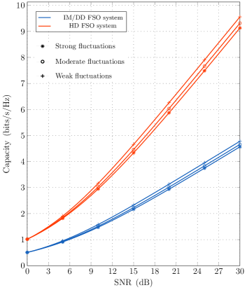
Figure 2: Capacity results for Gamma-Gamma turbulence channel without pointing error under HD and input-dependent IM-DD detection schemes. The average SNR at the receiver is the same as the transmit SNR since the average channel gain $\mathbb{E}[\lambda]\,=\,1$.

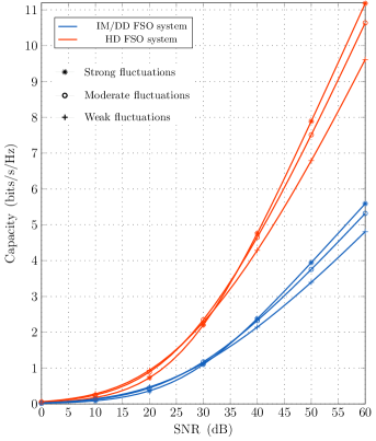
Figure 3: Capacity results for Gamma-Gamma turbulence channel with pointing jitter under HD and input-dependent IM-DD detection schemes. The (actual) average received SNR is lower than the transmit SNR by the factor $\mathbb{E}[\lambda]\,=\,A_{0}\,\xi^{2}/(1+\xi^{2})$ (see Remark 1). For example, for strong turbulence condition in Table I(b), the factor $A_{0}\,\xi^{2}/(1+\xi^{2})\approx-22.6$ (dB).

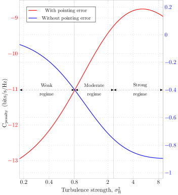
Figure 4: Capacity penalty at high SNR as a function of turbulence strength for the Gamma-Gamma turbulence channel with and without pointing jitter under HD detection scheme.

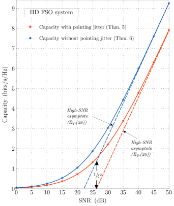
Figure 5: Capacity results for “Strong” Gamma-Gamma turbulence channels with and without pointing jitter under HD detection schemes (for fading parameters, see the third row in Table I(b)). Note that $A_{0}=0.0107$ is maintained for both exact and asymptotic results (see Remark 14) in both fading channels with and without pointing error.

Before proceeding with the numerical results, it is also important to note a key fundamental difference between the two FSO wireless systems, namely IM/DD and HD-based communication systems, that they have very different amount of noise power levels as discussed in the introduction section. The noise level in the direct detection (DD) receiver is generally very large due to the usage of optical filters (typically wideband) for signal or channel selection while the HD detection receiver employs sharp RF filters (with a lower noise level relatively) [6]. For simplicity and concreteness, we assume that the noise power levels (per Hz) in both detection receivers are the same, i.e., $N_{1}=N_{2}=N_{0}$, say. Note that $\mathrm{SNR}:=P_{\mathrm{avg}}/N_{0}$ is the average transmit SNR in all the derived capacity formulae (with subscript $k$ now suppressed from the SNR symbol in these capacity formulae as the noise levels are same) and also note that the horizontal axis in Figures 2$-$8 is the transmit SNR in log scale, not the received SNR. This is done to ensure a fair comparison between the two FSO detection schemes as well as to present a correct numerical analysis of the impact of varying atmospheric turbulence conditions and/or pointing errors. If required, the average received SNR can be computed by multiplying the transmit $\mathrm{SNR}$ and the mean channel (or irradiance) gain $\mathbb{E}[\lambda]$. Note that in all the figures to follow, we compute capacity (bits/sec/Hz is the unit of measurement) by multiplying the derived capacity by ${1}/{(\log 2)}$.

IV-C1 Exact capacity behavior

Firstly, the exact HD and IM/DD optical channel capacity values for the GG turbulence channel with and without pointing error are computed using Theorems 5 and 6 respectively and correspondingly plotted in Fig. 2 and Fig. 3. We have verified that these capacity values are in excellent agreement with the values obtained by numerically computing the (original) capacity integral (21) for different levels of atmospheric turbulence over a wide range of values of the SNR as displayed in Fig. 2 and Fig. 3.

Notice the capacity degradation with turbulence in Fig. 2 at high SNRs for both the detection schemes: the higher the turbulence strength, the greater the loss in capacity. This can be easily explained by noticing that the probability distribution of the channel gains (especially low gains) is severed with increasing turbulence conditions (refer Fig. 1). In the presence of pointing error, there is a sharp decline in the channel capacity performance as can be seen most clearly by comparing Fig. 2 and Fig. 3 in the high SNR regime; a quick heuristic argument to justify this is the reduction in the received SNR by a factor of $A_{0}\,\xi^{2}/(1+\xi^{2})$ as a consequence of pointing error.

But how exactly does the variation in atmospheric turbulence conditions and/or pointing error affect the capacity performance? The answer to this fundamental question is a bit involved, so we resort to analyzing the asymptotic capacity behavior in the high and low SNR regimes.

IV-C2 High SNR capacity behavior

The asymptotically tight (high-SNR) capacity result (30) in Theorem 7 suggests a constant difference with the $\log\mathrm{SNR}$ term (which is the AWGN capacity at high SNR). This difference, overall being negative-valued, can be interpreted as capacity penalty due to the combined effect of Gamma-Gamma fading and pointing jitter at high SNRs as follows:

$$\textrm{C}_{\textrm{penalty}}\,\triangleq\,\log\left(\dfrac{A_{0}}{ab}\right)+\psi(a)+\psi(b)-\frac{1}{\xi^{2}}.$$ (34)

Fig. 4 plots the capacity penalty (red curve) as a function of the strength of the atmospheric turbulence. We observe a startling fact that the capacity of a fixed-length GG fading channel improves with turbulence strength at high SNRs. To explain this, recall that we have considered a fixed-length horizontal FSO link with a collimated laser beam at the transmitter with the beam waist of $w_{0}=1.2$ cm (see Table I(b)). The beam footprint at the receiver (after propagating over $1.8$ km) is expanded due to atmospheric turbulence conditions. This enlarged beam size has two effects:

• it reduces the fraction of the power collected at the fixed-aperture receiver (i.e., $A_{0}$ reduces), and

• it accommodates the pointing jitter at the receiver more effectively (i.e., $\xi$ increases).

The beam enlargement due to greater turbulence yields an increase in capacity in the high SNR regime because the increase in accommodating pointing jitter more than compensates for the loss in collected power at the receiver, as shown in Fig. 4 for $\sigma_{\mathrm{R}}^{2}\,\leq\,6$. Eventually, for very strong turbulence conditions, the pointing jitter effect becomes negligible while the loss in collected power continues leading to capacity loss, as shown in Fig. 4 for $\sigma_{\mathrm{R}}^{2}\,>\,6$. We also note from Fig. 4 that the high-SNR penalty due to varying turbulence conditions can vary by a large amount (approximately $-13$ to $-8.5$ bits/s/Hz).

Remark 13.

It is important to note that the high-SNR penalty curve (red) in Fig. 4 is valid only for the considered FSO system and channel setting described in Table I(b). Keeping the FSO system parameters the same, a similar capacity penalty effect follows for other propagation path lengths; more penalty for shorter path lengths (in weak turbulence) and vice-versa.

Whereas in the Gamma-Gamma fading without pointing error, the penalty at high SNRs is described by (see (32))

$$C_{\textrm{penalty}}\,=\,\psi(a)+\psi(b)-\log\left(ab\right)$$ (35)

and is plotted as blue curve in Fig. 4. The Equation (35) can also be obtained from (34) by setting $A_{0}=1$ and $\xi\to\infty$ (see remark 2). Here, the penalty is monotonically increasing with turbulence strength and the extent of the penalty is relatively small (approximately $-0.9$ to $-0.1$ bits/s/Hz) in comparison with the penalty associated with both fading and pointing error (see Fig. 4).

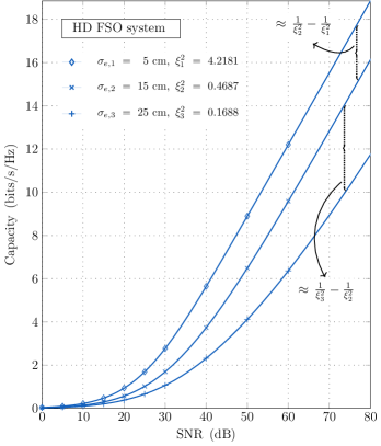
Figure 6: Capacity results for “Strong” Gamma-Gamma turbulence channel under HD detection scheme for varying levels of pointing jitter’s standard deviation $\sigma_{e}$ (or $\xi^{2}$ equivalently).

Remark 14.

In almost all the existing related works, the parameter $A_{0}$ is neglected for optical fading conditions without pointing error which is practically inaccurate; $A_{0}$ can in fact be a small fraction for a fading channel without pointing jitter problem. For a fair comparison, it is important to consider the impact of $A_{0}$ in both with and without pointing error cases.

In the ‘fixed-length’ optical channel with a fixed FSO system setting as we have considered, it is also possible to estimate the impact of increasing pointing jitter. Recall that $\sigma_{\mathrm{e}}$ is the pointing jitter’s standard deviation. The loss in capacity at high SNRs due to an increase in jitter (only) can be easily deduced and is given by

$$C_{\textrm{loss}}\,\approx\,({1}/{\xi^{2}_{\mathrm{new}}})-({1}/{\xi^{2}_{\mathrm{old}}})\,=\,4(\sigma_{\mathrm{e,\,new}}^{2}-\sigma_{\mathrm{e,\,old}}^{2})/w_{\mathrm{L_{eq}}}^{2}.$$ (36)

where $w_{\mathrm{L_{eq}}}$ is the (fixed) received equivalent beam waist. This is numerically illustrated in Fig. 6.

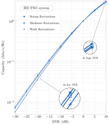
Figure 7: Ergodic capacity results at low SNR for Gamma-Gamma turbulence channel without pointing jitter under HD detection scheme (see Table I(b) for channel turbulence settings).

IV-C3 Low SNR capacity behavior

It is also interesting to see what happens to the spectral efficiency of the optical fading channel in the low-SNR regime. At low SNRs, the power control aspect of the transmitted laser beam becomes important which necessitates exploiting the higher fading gains efficiently.

In Fig. 7, we show the plot of the exact capacity versus SNR for the GG fading channel without pointing errors under the HD detection scheme. Somewhat surprisingly, the low-SNR capacity is showing improvement with increasing turbulence conditions. The exact reason is that the probability distribution of the higher channel gains improves with turbulence strength which is exploited by the transmitter operating at low SNR (with full CSI) to improve spectral efficiency. A similar low-SNR characteristic has been recently reported for the mobile RF single and double-fading channels in [39].

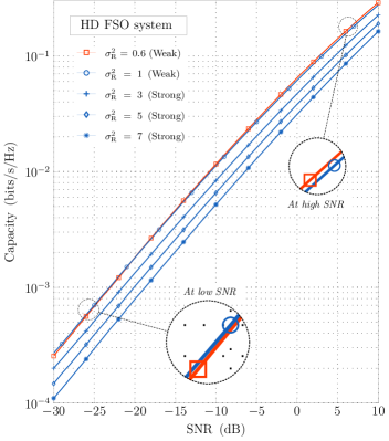
Figure 8: Ergodic capacity results at low SNR for Gamma-Gamma turbulence channel with pointing jitter under HD detection scheme.

On the other side, the impact of fading along with pointing error on the channel capacity at low SNRs becomes more involved. The exact capacity behavior at low SNRs is plotted in Fig. 8 for a wide range of turbulence conditions: the low-SNR capacity first shows improvement in the weak turbulence regime, and then, increasing turbulence leads to capacity degradation over the moderate-to-strong turbulence regime. This peculiar characteristic can also be explained exactly by understanding the probability distribution of higher channel gains (both fading and pointing error). Rather, we provide a quick explanation using the asymptotic results: from (31) in Theorem 7, the combined effect of both optical fading and pointing error on the channel capacity at low SNRs is summarily captured in $A_{0}/(4ab)$ and is termed as follows:

$$\textrm{Capacity scaling factor}\,\triangleq\,A_{0}\times\frac{1}{4ab}.$$ (37)

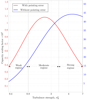
Figure 9: Capacity scaling factor at low SNR as a function of turbulence strength for the Gamma-Gamma turbulence channel with and without pointing jitter under HD detection scheme.

Fig. 9 plots the scaling factor (37) (red curve) as a function of the strength of the atmospheric turbulence along with the factor ${1}/{4ab}$ (blue curve). Comparing these two curves, we can see that the parameter $A_{0}$ (which indicates the fraction of collected power) degrades with turbulence (slowly in weak conditions and rapidly in strong conditions) while ${1}/{4ab}$ typically improves. Overall, except for weak conditions, the low-SNR capacity with both fading and pointing error typically degrades with turbulence strength over a wide range of moderate-to-strong conditions.

V Derivation of Exact Capacity in Theorem 5

The unified capacity expression (from (IV)) is summarized as

$$\widebar{C}\, =\,(I_{1}\,-\,I_{2}\,-\,I_{3})/k.$$ (38)

In the evaluation of the integrals $I_{1},\,I_{2}$ and $I_{3}$, we will repeatedly make use of the following identity  [40]:

$$\int x^{j-1}G_{p,q}^{m,n}\left(x\,\middle|\begin{array}[]{c}a_{1},\ldots,,a_{p}\\[1.00006pt] b_{1},\ldots,,b_{q}\end{array}\right)dx\,=\phantom{xxxxxxxxxxxxxxxxxxxxxxxxxxxx}$$ (41)

$$G^{m,\,n+1}_{p+1,\,q+1}\left(x\,\middle|\begin{array}[]{c}1,j+a_{1},\ldots,j+a_{n},j+a_{n+1},\ldots,j+a_{p}\\[1.00006pt] j+b_{1},\ldots,j+b_{m},0,j+b_{m+1},\ldots,j+b_{q}\end{array}\right).$$ (44)

The following subsections describe the calculus details involved in the evaluation of $I_{1},\,I_{2}$ and $I_{3}$.

V-A Evaluation of Integral $I_{1}$

The integral $I_{1}$ can be viewed as

$$I_{1}\,=\,\mathbb{E}\left[\log\lambda\right].$$ (45)

To evaluate (45), we use the relation $\frac{d}{dt}\lambda^{t}=\lambda^{t}\log(\lambda)$ and thereupon, taking expectation $\mathbb{E}[\cdot]$ on both sides for $t=0$ such that

$$\phantom{xxxxxxxxxxxx}\mathbb{E}\left[\lambda^{t}\log(\lambda)\right]\bigl{|}_{t=0}\,\,=\,\frac{d}{dt}\left(\mathbb{E}\left[\lambda^{t}\right]\right)\biggl{|}_{t=0}$$

$$\text{and hence}\phantom{xxxxxx}I_{1}\,=\,\frac{d}{dt}\left(\int_{0}^{\infty}\lambda^{t}f_{\lambda}(\lambda)d\lambda\right)\biggl{|}_{t=0}\,.$$ (46)

The $t$-th moment in the RHS of (V-A) is computed as follows:

$$\int_{0}^{\infty}\lambda^{t}f_{\lambda}(\lambda)d\lambda\,\,=$$

$$\frac{ab\xi^{2}}{A_{0}\Gamma(a)\Gamma(b)}\int_{0}^{\infty}\lambda^{t}\,G_{1,3}^{3,0}\left(\frac{ab\lambda}{A_{0}}\biggr{\rvert}\begin{array}[]{c}\xi^{2}\\ \xi^{2}-1,a-1,b-1\\ \end{array}\right)d\lambda.$$ (49)

Applying (41) in (V-A) along with the substitutions that

$$\lim_{x\to 0}\,\,G_{2,4}^{3,1}\left(x\,\biggr{\rvert}\begin{array}[]{c}1,\,\xi^{2}+t+1\\ \xi^{2}+t,\,a+t,\,b+t,\,0\\ \end{array}\right)\,=\,0,\,\,\,\text{and}$$

$$\lim_{x\to\infty}\,\,G_{2,4}^{3,1}\left(x\,\biggr{\rvert}\begin{array}[]{c}1,\,\xi^{2}+t+1\\ \xi^{2}+t,\,a+t,\,b+t,\,0\\ \end{array}\right)\,=\,\frac{\Gamma\left(a+t\right)\Gamma\left(b+t\right)}{\xi^{2}+t},$$

we have

$$I_{1}\,=\,\frac{\xi^{2}}{\Gamma(a)\Gamma(b)}\frac{d}{dt}\left(\left(\frac{A_{0}}{ab}\right)^{t}\frac{\Gamma\left(a+t\right)\Gamma\left(b+t\right)}{\xi^{2}+t}\right)\Biggl{|}_{t=0}.$$ (50)

Upon differentiation w.r.t. $t$ and then evaluating the attained expression with $t=0$, we obtain the final $I_{1}$ expression as

$$I_{1}\ =\ \log\left(\frac{A_{0}}{ab}\right)+\psi(a)+\psi(b)-\frac{1}{\xi^{2}}\,\cdot$$ (51)

In the above, we have used $d(\log\Gamma(x))/dx\,=\,\psi(x)$, where $\psi(\cdot)$ is the Euler’s Digamma function.

V-B Evaluation of Integral $I_{2}$

In order to compute $I_{2}$, we will first state a simple lemma that gives an (indefinite) integral identity involving the product of the $\log(\cdot)$ and the Meijer-G function.

Lemma 15.

$$\int\log(x)\,G_{p,q}^{m,n}\left(x\,\biggr{\rvert}\begin{array}[]{c}a_{1},\ldots,a_{p}\\[1.49994pt] b_{1},\ldots,,b_{q}\end{array}\right)dx\,=\,\log(x)\,\,\cdot\phantom{xxxxxxxxxxxxxxxxxxxxxxx}$$ (54)

$$G^{m,\,n+1}_{p+1,\,q+1}\left(x\,\biggr{\rvert}\begin{array}[]{c}1,a_{1}+1,\ldots,a_{n}+1,a_{n+1}+1,\ldots,a_{p}+1\\[1.49994pt] b_{1}+1,\ldots,b_{m}+1,0,b_{m+1}+1,\ldots,b_{q}+1\end{array}\right)\,-\,$$ (57)

$$G^{m,\,n+2}_{p+2,\,q+2}\left(x\,\biggr{\rvert}\begin{array}[]{c}1,1,a_{1}+1,\ldots,a_{n}+1,a_{n+1}+1,\ldots,a_{p}+1\\[1.49994pt] b_{1}+1,\ldots,b_{m}+1,0,0,b_{m+1}+1,\ldots,b_{q}+1\end{array}\right).$$ (60)

Proof:

Considering the LHS of (54), we apply the integration-by-parts technique treating $\log(\cdot)$ as the first function and the Meijer-G function as the second to get

$$\,\log(x)\int G_{p,q}^{m,n}\left(x\,\middle|\begin{array}[]{c}a_{1},\ldots,a_{p}\\[1.00006pt] b_{1},\ldots,b_{q}\end{array}\right)dx$$ (63)

$$-\int\frac{1}{x}\,\left(\int G_{p,q}^{m,n}\left({x}\,\middle|\begin{array}[]{c}a_{1},\ldots,a_{p}\\[1.00006pt] b_{1},\ldots,b_{q}\end{array}\right)d{x}\right)dx.$$ (66)

Applying the identity in (41) transposes (63) to the RHS in (54). This completes the proof. ∎

The integral part $I_{2}$ is now evaluated as follows:

$$I_{2}=\int_{0}^{\mu_{k}}\log(\lambda)f_{\lambda}(\lambda)d\lambda\phantom{xxxxxxxxxxxxxxxssssssssssssxx}\,$$

$$=\frac{ab\xi^{2}}{A_{0}\Gamma(a)\Gamma(b)}\int_{0}^{\mu_{k}}\log\left(\lambda\right)G_{1,3}^{3,0}\left(\frac{ab\lambda}{A_{0}}\biggr{\rvert}\begin{array}[]{c}\xi^{2}\\[1.00006pt] \xi^{2}-1,a-1,b-1\\ \end{array}\right)d\lambda$$ (69)

and using the lemma 15 to get

$$I_{2}\, =\,\biggl{[}\,G_{2,4}^{3,1}\left(\dfrac{ab\lambda}{A_{0}}\,\biggr{\rvert}\begin{array}[]{c}1,\xi^{2}+1\\[1.00006pt] \xi^{2},a,b,0\end{array}\right)\cdot\log(\lambda)$$ (72)

$$\,\,\,\,\,-G_{3,5}^{3,2}\left(\dfrac{ab\lambda}{A_{0}}\,\biggr{\rvert}\begin{array}[]{c}1,1,\xi^{2}+1\\[1.00006pt] \xi^{2},a,b,0,0\end{array}\right)\,\biggr{]}\,\biggl{|}_{\lambda=0}^{\lambda=\mu_{k}}\,\,\dfrac{\xi^{2}}{\Gamma(a)\Gamma(b)}.$$ (75)

With the following Meijer-G function limits:

$$\lim_{x\to 0}\,\, G_{2,4}^{3,1}\left(x\,\biggr{\rvert}\begin{array}[]{c}1,\xi^{2}+1\\[1.00006pt] \xi^{2},a,b,0\end{array}\right)\,\cdot\,\log(x)\,=\,0,\,\,\,\text{and}$$

$$\lim_{x\to 0}\,\, G_{3,5}^{3,2}\left(x\,\biggr{\rvert}\begin{array}[]{c}1,1,\xi^{2}+1\\[1.00006pt] \xi^{2},a,b,0,0\end{array}\right)\,=\,0,$$

the final $I_{2}$ expression is given by

$$I_{2}\, =\,\left[\,G_{2,4}^{3,1}\left(\dfrac{ab}{A_{0}}\mu_{k}\,\biggr{\rvert}\begin{array}[]{c}1,\xi^{2}+1\\[1.00006pt] \xi^{2},a,b,0\end{array}\right)\right.\cdot\log(\mu_{k})$$ (78)

$$\,\,\,-\left.G_{3,5}^{3,2}\left(\dfrac{ab}{A_{0}}\mu_{k}\,\biggr{\rvert}\begin{array}[]{c}1,1,\xi^{2}+1\\[1.00006pt] \xi^{2},a,b,0,0\end{array}\right)\,\right]\dfrac{\xi^{2}}{\Gamma(a)\Gamma(b)}.$$ (81)

V-C Evaluation of Integral $I_{3}$

The $I_{3}$ component is given as

$$I_{3}\, =\,\log(\mu_{k})\int_{\mu_{k}}^{\infty}f_{\lambda}(\lambda)d\lambda.\vspace*{-1em}$$ (82)

where the integral is computed as follows:

$$\int_{\mu_{k}}^{\infty}f_{\lambda}(\lambda)d\lambda\phantom{xxxxxxxxxxxxxxxxxxxxxxxxxxxxxxxxx}$$

$$=\,1-\frac{ab\xi^{2}}{A_{0}\Gamma(a)\Gamma(b)}\int^{\mu_{k}}_{0}G_{1,3}^{3,0}\left(\frac{ab\lambda}{A_{0}}\,\biggr{\rvert}\begin{array}[]{c}\xi^{2}\\[1.00006pt] \xi^{2}-1,a-1,b-1\\ \end{array}\right)d\lambda$$ (85)

$$=\,1-\frac{\xi^{2}}{\Gamma(a)\Gamma(b)}G_{2,4}^{3,1}\left(\frac{ab}{A_{0}}\mu_{k}\,\biggr{\rvert}\begin{array}[]{c}1,\,\xi^{2}+1\\[1.00006pt] \xi^{2},\,a,\,b,\,0\\ \end{array}\right).$$ (88)

The last equality is obtained by applying the identity in (41) along with the substitution that

$$\lim_{x\to 0}\,\,G_{2,4}^{3,1}\left(x\,\biggr{\rvert}\begin{array}[]{c}1,\,\xi^{2}+1\\[1.49994pt] \xi^{2},\,a,\,b,\,0\\ \end{array}\right)\,=\,0.$$

Substituting these $I_{1}$, $I_{2}$ and $I_{3}$ expressions back into (38) and consequent simplification gives the final closed-form expression of the capacity as summarized in the Theorem 5.

VI Derivation of The Asymptotic Capacity Results in Theorem 7

For the purpose of asymptotic capacity analysis, it is useful to derive $\mu_{k}\,-\,\mathrm{SNR}_{k}$ dependence from the average power constraint in the low and high SNR regimes.

Lemma 16.

For the optimal waterfilling allocation described by (19) for the transmitted laser beam intensity, the threshold satisfies

1. At high SNR: $\,\,\mu_{k}\,\approx\,\dfrac{1}{\mathrm{SNR}_{k}}$,
   

2. At  low SNR: $\,\,\,\,\mu_{k}\,\approx\,\dfrac{A_{0}}{4ab}\log^{2}\left(\dfrac{1}{\mathrm{SNR}_{k}}\right)$.

Proof:

Part 1): Substituting (10) into the average optical power constraint (20), we have

$$\dfrac{\mu_{k}\mathrm{SNR}_{k}}{A}\,=\,\int_{\mu_{k}}^{\infty}\left(1-\dfrac{\mu_{k}}{\lambda}\right)\,G_{1,3}^{3,0}\left(\frac{ab\lambda}{A_{0}}\,\biggr{\rvert}\begin{array}[]{c}\xi^{2}\\[1.00006pt] \xi^{2}-1,a-1,b-1\\ \end{array}\right)d\lambda$$

where $A\,:=\,{ab\xi^{2}/(A_{0}\Gamma(a)\Gamma(b)})$. Applying the identity in (41) to the power constraint equation stated above gives

$$\dfrac{\mu_{k}\mathrm{SNR}_{k}}{A}\,=\,\dfrac{1}{A}\,-\, \dfrac{A_{0}}{ab}G_{2,4}^{3,1}\left(\frac{ab}{A_{0}}\mu_{k}\,\biggr{\rvert}\begin{array}[]{c}1,\,\xi^{2}+1\\[1.00006pt] \xi^{2},\,a,\,b,\,0\\ \end{array}\right)$$ (91)

$$+\,\,\mu_{k}\, G_{2,4}^{3,1}\left(\dfrac{ab}{A_{0}}\mu_{k}\,\biggr{\rvert}\begin{array}[]{c}1,\xi^{2}\\[1.00006pt] \xi^{2}-1,a-1,b-1,0\end{array}\right).$$ (94)

With some effort, we can deduce from the power constraint (20) that $\mu_{k}$ bears a strictly monotone or one-to-one relation with $\mathrm{SNR}_{k}$ or more precisely, $\mu_{k}$ decreases inversely with increasing $\mathrm{SNR}_{k}$ and vice versa. We particularly note that the contributions from both the Meijer-G functions based terms in (91) for small input argument (due to high SNR values) are vanishingly small and hence

$$\lim_{\mu_{k}\to 0}\,\,\mu_{k}\mathrm{SNR}_{k}\,\,=\,\,1.\\$$

Part 2): To obtain an explicit expression for the $\mu_{k}\,-\,\mathrm{SNR}_{k}$ dependence in the low-SNR regime, we apply asymptotic low-order series expansion on the RHS of the average power constraint (20) giving

$$\mathrm{SNR}_{k}\,\approx\,K\,\cdot\,\mu_{k}^{\left(\frac{a+b}{2}\ -\frac{11}{4}\right)}e^{-2\sqrt{\frac{ab}{A_{0}}\mu_{k}}}$$ (95)

where $K$ is a positive constant independent of the threshold $\mu_{k}$ (the derivation of (95) is omitted due to space limitation).

Taking the logarithm on both sides of (95) and considering only the most significant term by the relative order of magnitude in the left-hand side above, we obtain

$$\log(\mathrm{SNR}_{k})\,\approx\,-2\sqrt{\tfrac{ab}{A_{0}}\mu_{k}}.$$ (96)

Solving (96) for $\mu_{k}$, we finally arrive at

$$\mu_{k}\,\approx\,\dfrac{A_{0}}{4ab}\log^{2}\left(\frac{1}{\mathrm{SNR}_{k}}\right).$$ (97)

This completes the proof of the second part. ∎

VI-A Low-SNR Asymptotics

The low-order series expansion of the Meijer-G function for large input argument $z$ (asymptotically $\infty$) is given by

$$G_{3,5}^{3,2}\left(z\ \biggr{\rvert}\ \begin{matrix}1,1,\xi^{2}+1\\ \xi^{2},a,b,0,0\end{matrix}\right)\,\approx\,e^{-2\sqrt{z}}\sqrt{\pi}\,z^{\frac{1}{4}(-7+2a+2b)}\\ +\frac{\Gamma(a)\Gamma(b)}{\xi^{2}}\left(\log(z)+\frac{1}{\xi^{2}}-\psi(a)-\psi(b)\right).$$ (98)

Substituting the above series expansion in (5), we observe

$$\widebar{C}\, \approx\,\,\tfrac{1}{k}\cdot K\,\cdot\,\mu_{k}^{\left(\frac{a+b}{2}\ -\frac{7}{4}\right)}e^{-2\sqrt{\frac{ab}{A_{0}}\mu_{k}}}.$$ (99)

Comparing (99) and (95), we find that

$$\widebar{C}\,\approx\,\,\tfrac{1}{k}\cdot\mu_{k}\,\mathrm{SNR}_{k}.$$ (100)

Finally, substituting $\mu_{k}$ from  (97) in (100) completes the proof of the low SNR capacity expansion (29) in Theorem 7.

VI-B High-SNR Asymptotics

At high SNR, the threshold follows $\mu_{k}\approx\mathrm{SNR}_{k}^{-1}$ (from lemma 16) while the Meijer’s G function becomes insignificant for small input argument (asymptotically $0$) as

$$\lim_{z\to 0}\,\,\,G_{3,5}^{3,2}\left(z\ \biggr{\rvert}\ \begin{matrix}1,1,\xi^{2}+1\\ \xi^{2},a,b,0,0\end{matrix}\right)\,=\,0.$$ (101)

With these substitutions in Theorem 5, the asymptotic high SNR capacity expression (30) in Theorem 7 is proved.

VII Concluding remarks

In this work, we presented a unified exact and asymptotic capacity analysis for existing FSO systems with adaptive power control mechanism operating in Gamma-Gamma atmospheric turbulence. The derived capacity formulas are more explicit: the impact of the fading, pointing error, and path-loss-related parameters can be easily identified, especially in extreme SNR regimes. Most notably, we have shown an interesting interplay between the pointing error parameters $A_{0}$ and $\xi^{2}$ with the variation in turbulence conditions: as the turbulence increases (from weak conditions), there is a rapid improvement in capacity in the high SNR regime because the reduction in the pointing jitter effect more than compensates for the loss in received power. Whereas for the fading channel without pointing errors, the capacity expectedly degrades with turbulence at high SNRs. We have also shown that at low SNR, the optical channel capacity improves with increasing turbulence conditions due to two reasons: the distribution of the higher fading gains improves with turbulence, and that the optical transmitter exploits higher fading gains more efficiently. But with pointing errors, the distribution of higher fading gains degrades severely with turbulence leading to capacity loss at low SNRs.

References

- [1] S. Arnon, J. Barry, G. Karagiannidis, R. Schober, and M. Uysal, Advanced Optical Wireless Communication Systems. Cambridge, U.K.: Cambridge Univ. Press, 2012.
- [2] Q. Liu, C. Qiao, G. Mitchell, and S. Stanton, “Optical wireless communication networks for first- and last-mile broadband access,” IEEE/OSA J. Opt. Netw., vol. 4, no. 12, p. 807–828, 2005.
- [3] D. Cornwell, “Laser communication from the Moon at 622Mb/s,” Available: http://spie.org/x107507.xml, 2014.
- [4] H. Haan and M. Tausendfreund, “Free-space optical data transmission for military and civil applications: A company report on technical solutions and market investigation,” in 2013 15th International Conference on Transparent Optical Networks (ICTON). IEEE, 2013, pp. 1–4.
- [5] D. J. Heatley, D. R. Wisely, I. Neild, and P. Cochrane, “Optical wireless: The story so far,” IEEE Commun. Mag., vol. 36, no. 12, pp. 72–74, 1998.
- [6] J. R. Barry and E. A. Lee, “Performance of coherent optical receivers,” Proceedings of the IEEE, vol. 78, no. 8, pp. 1369–1394, 1990.
- [7] L. C. Andrews, R. L. Phillips, and C. Y. Hopen, Laser Beam Scintillation with Applications. SPIE Press, Bellingham, Wash., 2001, vol. 99.
- [8] S. Bloom, E. Korevaar, J. Schuster, and H. Willebrand, “Understanding the performance of free-space optics,” Journal of Optical Networking, vol. 2, no. 6, pp. 178–200, 2003.
- [9] S. Arnon, “Effects of atmospheric turbulence and building sway on optical wireless-communication systems,” Opt. Lett., vol. 28, no. 2, pp. 129–131, Jan 2003.
- [10] L. C. Andrews and R. L. Phillips, Laser Beam Propagation Through Random Media: Second Edition. SPIE Press, Bellingham, Wash., 2005.
- [11] S. Karp, R. M. Gagliardi, S. E. Moran, and L. B. Stotts, Optical Channels: Fibers, Clouds, Water, and the Atmosphere. Springer Science & Business Media, 2013.
- [12] M. Al-Habash, L. C. Andrews, and R. L. Phillips, “Mathematical model for the irradiance probability density function of a laser beam propagating through turbulent media,” Optical Engineering, vol. 40, no. 8, pp. 1554–1562, 2001.
- [13] L. C. Andrews, R. L. Phillips, C. Y. Hopen, and M. Al-Habash, “Theory of optical scintillation,” JOSA A, vol. 16, no. 6, pp. 1417–1429, 1999.
- [14] A. A. Farid and S. Hranilovic, “Outage capacity optimization for free-space optical links with pointing errors,” Journal of Lightwave Technology, vol. 25, no. 7, pp. 1702–1710, 2007.
- [15] F. Yang, J. Cheng, and T. A. Tsiftsis, “Free-space optical communication with nonzero boresight pointing errors,” IEEE Transactions on Communications, vol. 62, no. 2, pp. 713–725, 2014.
- [16] M. A. Kashani, M. Uysal, and M. Kavehrad, “A novel statistical channel model for turbulence-induced fading in free-space optical systems,” Journal of Lightwave Technology, vol. 33, no. 11, pp. 2303–2312, 2015.
- [17] A. Jurado-Navas, J. M. Garrido-Balsells, J. F. Paris, A. Puerta-Notario, and J. Awrejcewicz, “A unifying statistical model for atmospheric optical scintillation,” in Numerical Simulations of Physical and Engineering Processes. Intech Rijeka, Croatia, 2011, vol. 181, no. 8, pp. 181–205.
- [18] D. Tse and P. Viswanath, Fundamentals of Wireless Communication. Cambridge, U.K.:: Cambridge University Press, 2005.
- [19] I. S. Ansari, M.-S. Alouini, and J. Cheng, “Ergodic capacity analysis of free-space optical links with nonzero boresight pointing errors,” IEEE Trans. Wirel. Commun., vol. 14, no. 8, pp. 4248–4264, 2015.
- [20] H. E. Nistazakis, E. A. Karagianni, A. D. Tsigopoulos, M. E. Fafalios, and G. S. Tombras, “Average capacity of optical wireless communication systems over atmospheric turbulence channels,” Journal of Lightwave Technology, vol. 27, no. 8, pp. 974–979, 2009.
- [21] W. Gappmair, “Further results on the capacity of free-space optical channels in turbulent atmosphere,” IET Communications, vol. 5, no. 9, pp. 1262–1267, 2011.
- [22] I. S. Ansari, F. Yilmaz, and M.-S. Alouini, “Performance analysis of FSO links over unified gamma-gamma turbulence channels,” in IEEE 81st Vehicular Technology Conference (VTC Spring), 2015, pp. 1–5.
- [23] A. Lapidoth, S. M. Moser, and M. A. Wigger, “On the capacity of free-space optical intensity channels,” IEEE Transactions on Information Theory, vol. 55, no. 10, pp. 4449–4461, 2009.
- [24] S. M. Moser, “Capacity results of an optical intensity channel with input-dependent Gaussian noise,” IEEE Transactions on Information Theory, vol. 58, no. 1, pp. 207–223, 2012.
- [25] S. Bloom et al., “The physics of free-space optics,” AirFiber Inc. White Paper, pp. 1–22, 2002.
- [26] I. S. Gradshteyn and I. M. Ryzhik, Table of Integrals, Series, and Products, 7th ed. San Diego, CA: Academic Press, Inc., 2007.
- [27] H. Weichel, Laser Beam Propagation in the Atmosphere. SPIE Optical Engineering Press, Bellingham, 1990.
- [28] B. E. Saleh and M. C. Teich, Fundamentals of Photonics. John Wiley & Sons, Ltd, 2019.
- [29] R. R. Beland, Propagation through Atmospheric Optical Turbulence. The Infrared and ElectroOptical Systems Handbook, F. G. Smith, ed. (SPIE Optical Engineering Press, Bellingham, Washington), 1993, vol. 2.
- [30] A. A. Farid and S. Hranilovic, “Outage capacity optimization for free-space optical links with pointing errors,” Journal of Lightwave Technology, vol. 25, no. 7, pp. 1702–1710, 2007.
- [31] J. C. Ricklin and F. M. Davidson, “Atmospheric turbulence effects on a partially coherent Gaussian beam: implications for free-space laser communication,” J. Opt. Soc. Amer. A, Opt. Image Sci., vol. 19, no. 9, pp. 1794–1802, Sept. 2002.
- [32] M. Miao, X.-y. Chen, R. Yin, and J. Yuan, “New results for the pointing errors model in two asymptotic cases,” IEEE Photonics Journal, vol. 15, no. 3, pp. 1–7, 2023.
- [33] K. Kikuchi, “Fundamentals of coherent optical fiber communications,” Journal of Lightwave Technology, vol. 34, no. 1, pp. 157–179, 2015.
- [34] G. P. Agrawal, Fiber-Optic Communication Systems, 3rd ed. New York: Wiley, 2002.
- [35] A. Chaaban, Z. Rezki, and M.-S. Alouini, “On the capacity of intensity-modulation direct-detection Gaussian optical wireless communication channels: A tutorial,” IEEE Communications Surveys & Tutorials, vol. 24, no. 1, pp. 455–491, 2021.
- [36] E. A. Lee and D. G. Messerschmitt, Digital Communication. Springer Science & Business Media, 2012.
- [37] I. E. Lee, Z. Ghassemlooy, W. P. Ng, M.-A. Khalighi, and S.-K. Liaw, “Effects of aperture averaging and beam width on a partially coherent Gaussian beam over free-space optical links with turbulence and pointing errors,” Applied Optics, vol. 55, no. 1, pp. 1–9, 2016.
- [38] X. Tang, Z. Ghassemlooy, W. O. Popoola, and C. G. Lee, “Coherent polarization shift keying modulated free space optical links over a gamma-gamma turbulence channel,” American Journal of Engineering and Applied Sciences, vol. 4, no. 4, pp. 520–530, 2011.
- [39] K. Singh, “On the capacity of low-rank dyadic fading channels in the Low-SNR regime,” Available: https://arxiv.org/abs/2308.05078, 2023.
- [40] Wolfram Research, Inc., “The Wolfram Functions site,” Available: https://functions.wolfram.com/07.34.21.0002.01, [Accessed 29-May-2023].