Dynamical system analysis of DBI scalar field cosmology in coincident $f(Q)$ gravity

Abstract

In this article, we offer the dynamical system analysis of the DBI (Dirac-Born-Infeld) scalar field in a modified $f(Q)$ gravity context. We have taken a polynomial form of modified gravity and used two different kinds of scalar potential, i.e., polynomial and exponential, and found a closed autonomous dynamical system of equations. We have analyzed the fixed points of such a system and commented on the conditions under which deceleration to late-time acceleration happens in this model. We have noted the similarity of the two models and have also shown that our result is indeed consistent with the previous work done on Einstein’s gravity. We have also investigated the phenomenological implications of our models by plotting the EoS ($\omega$), Energy density ($\Omega$), and deceleration parameter ($q$) w.r.t. to e-fold time and comparing with the present value. Finally, we conclude the paper by observing how the dynamical system analysis differs in modified $f(Q)$ gravity, and we also provide some of the future scope of our work.

Keywords: Scalar field, $f(Q)$ gravity, dark energy, dynamical system analysis.

I Introduction

After the discovery of CMB (Cosmic microwave background), it became clear that our universe started in a very hot, dense state and has remained in its current form. This is known as the standard Big Bang theory of cosmology. After the discovery of late time acceleration [1, 2] and observation from the galaxy rotation curve, it has been clear that there are other objects in our universe except for baryonic matter. In the standard $\Lambda$CDM paradigm, which is probably the most successful theory about the current state of the universe, one takes dark energy (which is responsible for late time acceleration) as Cosmological constant $\Lambda$ and dark matter to be cold (non-radiative). Even though the $\Lambda$CDM model is so successful with phenomenological predictions and observational evidence, it has some severe problems. One of the main problems is the nature of dark energy. If one assumes that cosmological constant ($\Lambda$) is solely responsible for dark energy, then calculations from QFT can be shown to have a discrepancy of order ($10^{120}$). One natural way to explain this is by introducing the scalar field (Quintessence field), which can explain why the current value of the cosmological constant is so low. The scalar field also appears quite naturally in the early inflation scenarios, which can naturally explain the horizon problem and flatness problem, etc.
Even though the scalar field can explain both early inflation and late-time acceleration, the exact form or the origin of the scalar field is not known. There are many such candidates for the origin of the inflation or quintessence fields. In this article, we take Dirac-Born-Infeld (DBI) as the origin of the scalar field, which naturally comes from the string theory. We have also done a dynamical system analysis in the flat FLRW background and given the phenomenological predictions (evolution graph of $q$, $\Omega$, $\omega$) based on the fixed point analysis.
It is well known that Einstein’s general theory of relativity is not renormalizable in the context of quantum field theory. There have been several attempts to find a renormalizable theory of quantum gravity, and string theory offers one such unification. It is well known that even in bosonic string theory, the quantization Polyakov action (conformal transformation of Nambu-Goto action) gives tachyon like a field which soon decays via spontaneous symmetry breaking [3, 4]. It was first observed by Mazumdar et al. [5] that the decay of a non-BPS $D4$ branes to a stable $D3$ branes can give rise to tachyon field, which can act as an inflation field in the cosmological context. In 2002, a series of three papers by Sen [6, 7, 8] showed how in string theory as well as in string field theory, tachyons occur naturally, and in [8] it has been shown that the effective field of such tachyons can be viewed as DBI scalar field theory.
Soon after these proposals, Padmanabhan [9] and Gibbons [10] showed how these DBI-type fields could be used in the FLRW background to give inflation field-like behaviour. Alternative ways of getting the DBI field from other forms of string theory have been reviewed by Gibbons [11]. The study of the DBI field in late time acceleration context has been done by Bhagla et al. [12], while Gorini et al.[13]) offered the alternative way of visualizing the DBI field as a modified Chaplygin gas. We also note that DBI field has been proposed as an alternative to dark matter by Padmanabhan [14].
Copeland [15] and Aguirregabiria [16] first studied the study of the DBI field in the dynamical system setting. In this paper also, we are closely following the treatment given in [15]. Soon after that, Fang and Lu [17] considered a much more general type of potential beyond inverse square potential, the work later extended by Quiros et al. [18] to include much more general potentials, and they have given an exact treatment of $sinh(\phi)$ potential. Guo [19] has chosen an exponential potential for dynamical system analysis. It is also worth noting that as Silversteinand Tong [20] have shown, if one considers a D3-brane moving towards the horizon of AdS space, one can get a generalized DBI field in a strong coupling limit (as opposed to a weak coupling limit where the previous work has been done). In strong coupling limit, it can shown that DBI field gets extra contributions from the movement of the D3-brane and the lagrangian becomes $\mathcal{L}_{GDBI}=\frac{1}{f(\phi)}(\sqrt{1+f(\phi)\partial\phi^{2}}-1)-V(\phi)$.
The general criteria for the DBI field to give de-Sitter-like later time acceleration is given by the theorem of Hao[21] and Chingangbam [22]. Furthermore, the conventional concept of relativity, especially General Relativity, which interprets gravity as the curvature of spacetime, may not offer the definitive solution to elucidate dark energy. This encourages the exploration of alternative theoretical frameworks in cosmology that can effectively address cosmic acceleration while remaining consistent with observational data. General Relativity and its curvature-based extensions have been formulated and thoroughly examined in previous research [23, 24]. Recently, alternative theories of gravitation based on a flat spacetime geometry, relying solely on non-metricity, have been established and extensively explored [25, 26]. The $f(Q)$ gravity, with its various astrophysical and cosmological implications, has been widely investigated [27, 28, 29, 30, 31, 32, 33, 34, 35, 36, 37, 38]. In this article, we have shown that even with the modified $f(Q)$ gravity, we are getting a similar kind of late-time accelerating behaviour where $q$ is $-1$ as expected from de-Sitter-like expansion. We also note that in our model, the value of is coming very close to $-0.6$, which is very close to the currently accepted value of $q$.

II $f(Q)$ gravity formulation with scalar field

We begin with the fact that a connection plays a vital role in transporting tensors across a manifold. In the realm of general relativity, which is built upon Riemannian geometry, the gravitational interactions are ruled by a symmetric connection referred to as the Levi-Civita connection. Nevertheless, a more generic connection comprises two components: an antisymmetric part and another component exhibiting the non-metricity condition. This extended affine connection can be expressed as follows [39]:

$$\Upsilon^{\alpha}_{\ \mu\nu}=\Gamma^{\alpha}_{\ \mu\nu}+K^{\alpha}_{\ \mu\nu}+L^{\alpha}_{\ \mu\nu},$$ (1)

where the first term denotes the metric-compatible Levi-Civita connection,

$$\Gamma^{\alpha}_{\ \mu\nu}\equiv\frac{1}{2}g^{\alpha\lambda}(g_{\mu\lambda,\nu}+g_{\lambda\nu,\mu}-g_{\mu\nu,\lambda})$$ (2)

The second one is the contortion tensor representing the antisymmetric part of the affine connection, and that can be estimated in terms of the torsion tensor $T^{\alpha}_{\ \mu\nu}\equiv\Upsilon^{\alpha}_{\ \mu\nu}-\Upsilon^{\alpha}_{\ \nu\mu}$ as follows,

$$K^{\alpha}_{\ \mu\nu}\equiv\frac{1}{2}(T^{\alpha}_{\ \mu\nu}+T_{\mu\ \nu}^{\ \alpha}+T_{\nu\ \mu}^{\ \alpha})$$ (3)

, and the last one is the distortion tensor,

$$L^{\alpha}_{\ \mu\nu}\equiv\frac{1}{2}(Q^{\alpha}_{\ \mu\nu}-Q_{\mu\ \nu}^{\ \alpha}-Q_{\nu\ \mu}^{\ \alpha})$$ (4)

which is expressed in terms of non-metricity tensor,

$$Q_{\alpha\mu\nu}\equiv\nabla_{\alpha}g_{\mu\nu}=\partial_{\alpha}g_{\mu\nu}-\Upsilon^{\beta}_{\,\,\,\alpha\mu}g_{\beta\nu}-\Upsilon^{\beta}_{\,\,\,\alpha\nu}g_{\mu\beta}$$ (5)

In addition, we define the superpotential tensor as

$$4P^{\lambda}\>_{\mu\nu}=-Q^{\lambda}\>_{\mu\nu}+2Q_{(\mu}\>^{\lambda}\>{}_{\nu)}+(Q^{\lambda}-\tilde{Q}^{\lambda})g_{\mu\nu}-\delta^{\lambda}_{(\mu}Q_{\nu)}.$$ (6)

where $Q_{\alpha}=Q_{\alpha}\>^{\mu}\>{}_{\mu}$ and $\tilde{Q}_{\alpha}=Q^{\mu}\>_{\alpha\mu}$ are non-metricity vectors. Now, by contracting the superpotential tensor with the non-metricity tensor, we obtain the non-metricity scalar in a more concise form,

$$Q=-Q_{\lambda\mu\nu}P^{\lambda\mu\nu}.$$ (7)

We know that the curvature tensor can be estimated as

$$R^{\alpha}_{\>\beta\mu\nu}=2\partial_{[\mu}\Upsilon^{\alpha}_{\>\nu]\beta}+2\Upsilon^{\alpha}_{\>[\mu\mid\lambda\mid}\Upsilon^{\lambda}_{\nu]\beta}$$ (8)

Now by using the affine connection (1), one can have

$$R^{\alpha}_{\>\beta\mu\nu}=\mathring{R}^{\alpha}_{\>\beta\mu\nu}+\mathring{\nabla}_{\mu}X^{\alpha}_{\>\nu\beta}-\mathring{\nabla}_{\nu}X^{\alpha}_{\>\mu\beta}+X^{\alpha}_{\>\mu\rho}X^{\rho}_{\>\nu\beta}-X^{\alpha}_{\>\nu\rho}X^{\rho}_{\>\mu\beta}$$ (9)

Here $\mathring{R}^{\alpha}_{\>\beta\mu\nu}$ and $\mathring{\nabla}$ are described in terms of the Levi-Civita connection (2), and $X^{\alpha}_{\ \mu\nu}=K^{\alpha}_{\ \mu\nu}+L^{\alpha}_{\ \mu\nu}$. On applying suitable contractions on curvature term and torsion-free constraint $T^{\alpha}_{\ \mu\nu}=0$ in the equation (9), we have

$$R=\mathring{R}-Q+\mathring{\nabla}_{\alpha}\left(Q^{\alpha}-\tilde{Q}^{\alpha}\right)$$ (10)

where $\mathring{R}$ is the usual Ricci scalar evaluated regarding the Levi-Civita connection. Further on employing teleparallel constraint $R=0$, we acquire curvature free teleparallel geometries, and hence relation (10) becomes

$$\mathring{R}=Q-\mathring{\nabla}_{\alpha}\left(Q^{\alpha}-\tilde{Q}^{\alpha}\right)$$ (11)

The relation obtained in the equation (11) indicates that the Ricci scalar curvature differs from the non-metricity scalar by a boundary term. The equation (11) reveals that the gravity theory incorporates only non-metricity scalar $Q$ in the action, which differs from Einstein’s GR by a boundary term. This indicates that STEGR presents an equivalent formulation to GR, and hence, the theory is known as a symmetric teleparallel equivalent to GR [40].

Now, we present the action for $f(Q)$ gravity, which is a generalization to STEGR theory, in the presence of a scalar field,

$$\mathcal{S}=\int\frac{1}{2}\,f(Q)\sqrt{-g}\,d^{4}x+\int\mathcal{L}_{\phi}\,\sqrt{-g}\,d^{4}x\,,$$ (12)

where $g=\text{det}(g_{\mu\nu})$, $f(Q)$ is an arbitrary function of the non-metricity scalar $Q$, and $\mathcal{L}_{\phi}$ is the Lagrangian density of a scalar field $\phi$ given by [41],

$$\mathcal{L}_{\phi}=-\frac{1}{2}g^{\mu\nu}\partial_{\mu}\phi\partial_{\nu}\phi-V(\phi)$$ (13)

Here $V(\phi)$ represents a potential for the field $\phi$. We obtain the following governing field equation by varying the action (12) with respect to the metric,

$$\frac{2}{\sqrt{-g}}\nabla_{\lambda}(\sqrt{-g}f_{Q}P^{\lambda}\>_{\mu\nu})+\frac{1}{2}g_{\mu\nu}f+f_{Q}(P_{\mu\lambda\beta}Q_{\nu}\>^{\lambda\beta}-2Q_{\lambda\beta\mu}P^{\lambda\beta}\>_{\nu})=-T_{\mu\nu}^{\phi}$$ (14)

where $f_{Q}=\frac{df}{dQ}$ and $T_{\mu\nu}^{\phi}$ represents the stress-energy tensor of the scalar field given as

$$T_{\mu\nu}^{\phi}=\partial_{\mu}\phi\partial_{\nu}\phi-\frac{1}{2}g_{\mu\nu}g_{\alpha\beta}\partial^{\alpha}\phi\partial^{\beta}\phi-g_{\mu\nu}V(\phi)$$ (15)

Moreover, we obtain the following equation of motion for the scalar field i.e. Klein-Gordon equation from the Euler-Lagrangian equation for the Lagrangian density given by (13)

$$\square\phi-V,_{\phi}=0$$ (16)

Here $\square$ denotes the d’Alembertian and $V,_{\phi}=\frac{\partial V}{\partial\phi}$. Further, on varying the action (12) with respect to the connection (similar to Palatini prescription), we have,

$$\nabla_{\mu}\nabla_{\nu}(\sqrt{-g}f_{Q}P^{\mu\nu}\>_{\lambda})=0$$ (17)

III Equations of Motion

We begin with the following flat FLRW line element to probe the cosmological implications under the assumption of spatial isotropy and homogeneity of the universe,

$$ds^{2}=-dt^{2}+a^{2}(t)[dx^{2}+dy^{2}+dz^{2}]$$ (18)

Here $a(t)$ is a measure of the universe’s expansion. Beginning with the teleparallel constraint that corresponds to a flat geometry characterizing a pure inertial connection, one can execute a gauge transformation parameterized by $\Lambda^{\alpha}_{\mu}$ [42],

$$\Upsilon^{\alpha}_{\>\mu\nu}=(\Lambda^{-1})^{\alpha}_{\>\>\beta}\partial_{[\mu}\Lambda^{\beta}_{\>\>\nu]}$$ (19)

Consequently, one can express the generic affine connection in the following manner, by utilizing the general element of $GL(4,\mathbb{R})$ characterized by the transformation $\Lambda^{\alpha}_{\>\>\mu}=\partial_{\mu}\zeta^{\alpha}$, where $\zeta^{\alpha}$ is an arbitrary vector field,

$$\Upsilon^{\alpha}_{\>\mu\nu}=\frac{\partial x^{\alpha}}{\partial\zeta^{\rho}}\partial_{\mu}\partial_{\nu}\zeta^{\rho}$$ (20)

This reveals the possibility of eliminating the connection through a coordinate transformation. The coordinate transformation is responsible for eliminating the connection (20) is termed gauge coincident. We utilize the coincident gauge in the present manuscript. Hence, the non-metricity scalar corresponds to the metric (18) becomes $Q=6H^{2}$.
The stress-energy tensor for the perfect fluid distribution reads as

$$T_{\mu\nu}=(\rho+p)u_{\mu}u_{\nu}+pg_{\mu\nu}$$ (21)

where we have taken $u^{\mu}=(1,0,0,0)$ are components of the four velocities. On comparing equation (21) and (15), we have,

$$\rho=-\frac{1}{2}g_{\alpha\beta}\partial^{\alpha}\phi\partial^{\beta}\phi+V(\phi)$$ (22)

$$p=-\frac{1}{2}g_{\alpha\beta}\partial^{\alpha}\phi\partial^{\beta}\phi-V(\phi)$$ (23)

As the scalar field considered here does not depend on the spatial coordinates, we have following expressions for the energy density and pressure component of the scalar field,

$$\rho_{\phi}=\frac{1}{2}\dot{\phi}^{2}+V(\phi)$$ (24)

$$p_{\phi}=\frac{1}{2}\dot{\phi}^{2}-V(\phi)$$ (25)

and the corresponding equation of state parameter can be written as,

$$\omega_{\phi}=\frac{p_{\phi}}{\rho_{\phi}}=\frac{\frac{1}{2}\dot{\phi}^{2}-V(\phi)}{\frac{1}{2}\dot{\phi}^{2}+V(\phi)}$$ (26)

Moreover, corresponding to the metric (18), the Klein-Gordon equation (16) becomes,

$$\ddot{\phi}+3H\dot{\phi}+V_{,\phi}=0$$ (27)

We obtain the following Friedmann-like equations governing the gravitational interactions under the $f(Q)$ gravity background in the presence of a scalar field,

$$3H^{2}=\frac{1}{2f_{Q}}\left(-\rho_{\phi}+\frac{f}{2}\right)$$ (28)

$$\dot{H}+3H^{2}+\frac{\dot{f_{Q}}}{f_{Q}}H=\frac{1}{2f_{Q}}\left(p_{\phi}+\frac{f}{2}\right)$$ (29)

For the $f(Q)$ functional $f(Q)=-Q+\Psi(Q)$, we can rewrite the Friedmann equations (28)-(29) as (where we can recover ordinary GR by putting $\Psi=0$)

$$3H^{2}=\rho_{\phi}+\rho_{de}$$ (30)

$$\dot{H}=-\frac{1}{2}[\rho_{\phi}+p_{\phi}+\rho_{de}+p_{de}]$$ (31)

where $\rho_{de}$ and $p_{de}$ represent the energy density and pressure of the dark energy component evolving due to the geometry of spacetime,

$$\rho_{de}=-\frac{\Psi}{2}+Q\Psi_{Q}$$ (32)

$$p_{de}=-\rho_{de}-2\dot{H}\left(\Psi_{Q}+2Q\Psi_{QQ}\right)$$ (33)

IV The Cosmological Model and Dynamical System Analysis

One of the main troubles of using string theory in cosmology directly is the so-called no-go theorem (gibbon), for wrapped products done by compactifying the extra dimensions. We note that from the equations below the dynamical system equations, we can see that it does not get closed for generalized DBI field but closed for ordinary DBI but in order to get the critical points at infinity, we need to compactify the phase space, which we did in 12 number equation.
In string theory, it was predicted by Sen [6, 7, 8] there are tachyon fields in both open and closed string theory. Even though for closed string theory, the tachyon fields are projected out in open string, they remain even though one can use a spontaneous symmetry-breaking argument to get rid of tachyon modes, one can still fully explain the reason for its existence. in the bosonic string theory if one uses Nambu- Goto action then it is almost impossible to quantize in order to get meaningful quantization rules one has to invoke the conformal invariant Polyakov action, using the conformal field theory techniques one can quantize such an action which leads to the undesirable tachyon modes, even though they violate casualty it can be shown that they are unstable. So Tachyon modes are typically given by Dirac-Born-Infeld (DBI) Lagrangian, which have the following form,

$$\mathcal{L}_{Tachyon}=V(\phi)\sqrt{1+\partial\phi^{2}\partial^{\mu}\phi\partial_{\mu}\phi}$$ (34)

Where $\partial\phi^{2}=\partial^{\mu}\phi\partial_{\mu}\phi$ and $V(\phi)$ is a potential function for the scalar field and $\partial^{\mu}\phi\partial_{\mu}\phi$ denotes the kinetic term for tachyon fields,
From the Lagrangian, one can find the field equation for the Tachyon field from the Euler-Lagrangian equation as,

$$\frac{\ddot{\phi}}{1-\dot{\phi}^{2}}+3H\dot{\phi}+\frac{V_{,\phi}}{V}=0$$ (35)

This is the modified Klein-Gordon equation for the DBI field.
Cosmological (freedman equations) equations become,

$$3H^{2}=\rho+\frac{V}{\sqrt{1-\dot{\phi}^{2}}}$$ (36)

We note that for such cases the energy density ($\rho$) and pressure ($p$) are given by,

$$\rho_{\phi}=\frac{V}{\sqrt{1-\dot{\phi}^{2}}}$$ (37)

$$p_{\phi}=-V\sqrt{1-\dot{\phi}^{2}}$$ (38)

so the equation of state ($\omega_{\phi}$) is given by

$$\omega_{\phi}=\frac{p_{\phi}}{\rho_{\phi}}=\phi^{2}-1$$ (39)

In order to construct the autonomous dynamical system, we use the following. We can define the variables as $x=\dot{\phi}$ and $y=\frac{\sqrt{V}}{\sqrt{3}H}$ so we can write $x^{2}=\dot{\phi}^{2}$ and $y^{2}\frac{V}{3H^{2}}$ and $s^{2}=\Omega_{de}=\frac{\rho_{de}}{3H^{2}}$.
So from 36 we get

$$3H^{2}= \rho_{\phi}+\rho_{de}$$ (40)

$$3H^{2}= \frac{V}{\sqrt{1-\dot{\phi}^{2}}}+\rho_{de}$$ (41)

$$1= \frac{V}{3H^{2}}\frac{1}{\sqrt{1-\dot{\phi}^{2}}}+\frac{\rho_{de}}{3H^{2}}$$ (42)

$$1= \frac{y^{2}}{\sqrt{1-x^{2}}}+s^{2}$$ (43)

$$s^{2}= 1-\frac{y^{2}}{\sqrt{1-x^{2}}}$$ (44)

As we know $x=\dot{\phi}$ which implies $\dot{x}=\ddot{\phi}$. We note that in order to form the dynamical system , it is more convenient to take the ”e-folding” timing defined as $N=\ln a$ so we get $\frac{d}{dt}=\frac{d}{dN}H$
As $\dot{x}=\ddot{\phi}$ we can write $x^{\prime}=\frac{\ddot{\phi}}{H}$. (where $\prime$ denotes the derivative with respect to ”e-folding” time and $\dot{}$ denotes the derivative with respect to ordinary time.)
From the Klein-Gordon equation for the DBI field, we get,

$$\frac{\ddot{\phi}}{1-\dot{\phi}^{2}}+3H\dot{\phi}+\frac{V_{,\phi}}{V}= 0$$ (45)

$$\frac{\ddot{\phi}}{1-\dot{\phi}^{2}}= -3H\dot{\phi}-\frac{V_{,\phi}}{V}$$ (46)

$$\ddot{\phi}= (1-\dot{\phi}^{2})[-3H\dot{\phi}-\frac{V_{,\phi}}{V}]$$ (47)

$$\ddot{\phi}= (1-\dot{\phi}^{2})[-3Hx+\lambda V^{\frac{1}{2}}]$$ (48)

$$\ddot{\phi}= (1-x^{2})[\lambda V^{\frac{1}{2}}-3Hx]$$ (49)

where we have defined $\lambda$ as $\lambda=-\frac{V_{,\phi}}{V^{\frac{3}{2}}}$. Now we note,

$$x^{\prime}= \frac{\ddot{\phi}}{H}$$ (50)

$$x^{\prime}= \frac{1}{H}(1-x^{2})(\lambda V^{\frac{1}{2}}-3Hx)$$ (51)

$$x^{\prime}= (1-x^{2})(\frac{\lambda\sqrt{V}}{H}-3x)$$ (52)

$$x^{\prime}= (x^{2}-1)(3x-\sqrt{3}\lambda y)$$ (53)

Where we have used the fact that $y=\frac{\sqrt{V}}{\sqrt{3}H}$. We also note that as $y^{2}=\frac{V}{3H^{2}}$ we can get the following,

$$y^{2}= \frac{V}{3H^{2}}$$ (54)

$$2y\dot{y}= \frac{\dot{V}}{3H^{2}}-\frac{2V\dot{H}}{3H^{3}}$$ (55)

$$\dot{y}= \frac{1}{2y}[\frac{\dot{V}}{3H^{2}}-\frac{2V\dot{H}}{3H^{3}}]$$ (56)

$$y^{\prime}= \frac{1}{2y}[\frac{\dot{V}}{3H^{3}}-2y^{2}\frac{\dot{H}}{H^{2}}]$$ (57)

We also note that $\dot{V}=V_{\phi}\dot{\phi}$ so we can write,

$$y^{\prime}= \frac{1}{2y}[\frac{V_{,\phi}\dot{\phi}}{3H^{3}}-2y^{2}\frac{\dot{H}}{H^{2}}]$$ (58)

$$= \frac{1}{2y}[\frac{-\lambda V^{\frac{3}{2}}}{3H^{3}}x-2y^{2}\frac{\dot{H}}{H^{2}}]$$ (59)

$$= -\frac{1}{2}y[\frac{\lambda x\sqrt{V}}{H}+2\frac{\dot{H}}{H^{2}}]$$ (60)

$$y^{\prime}= -\frac{1}{2}y[\sqrt{3}\lambda xy+2\frac{\dot{H}}{H^{2}}]$$ (61)

For the declaration parameter, we use the following,

$$-\frac{2\dot{H}}{3H^{2}}= \frac{\rho_{phi}}{3H^{2}}+\frac{\rho_{de}}{3H^{2}}+\frac{p_{\phi}}{3H^{2}}+\frac{p_{de}}{3H^{2}}$$ (62)

$$\frac{2\dot{H}}{3H^{2}}= 1-\frac{V\sqrt{1-\dot{\phi}^{2}}}{3H^{2}}-\frac{\rho_{de}}{3H^{2}}-\frac{2\dot{H}}{3H^{2}}(\Psi_{Q}+2Q\Psi_{QQ})$$ (63)

$$\frac{2\dot{H}}{3H^{2}}[\Psi_{Q}+2Q\Psi_{QQ}-1]= 1-y^{2}\sqrt{1-x^{2}}-s^{2}$$ (64)

$$\frac{2\dot{H}}{3H^{2}}[\Psi_{Q}+2Q\Psi_{QQ}-1]= 1-y^{2}\sqrt{1-x^{2}}-1+\frac{y^{2}}{\sqrt{1-x^{2}}}$$ (65)

$$\frac{2\dot{H}}{3H^{2}}[\Psi_{Q}+2Q\Psi_{QQ}-1]= \frac{x^{2}y^{2}}{\sqrt{1-x^{2}}}$$ (66)

$$\frac{\dot{H}}{H^{2}}= \frac{3x^{2}y^{2}}{2\sqrt{1-x^{2}}[\Psi_{Q}+2Q\Psi_{QQ}-1]}$$ (67)

So the deceleration parameter ($q$) is given by,

$$q=-1-\frac{3x^{2}y^{2}}{2\sqrt{1-x^{2}}[\Psi_{Q}+2Q\Psi_{QQ}-1]}$$ (68)

From the equation of $y^{\prime}$ we get,

$$y^{\prime}= -\frac{1}{2}y[\sqrt{3}\lambda xy+2\frac{\dot{H}}{H^{2}}]$$ (69)

$$y^{\prime}= -\frac{1}{2}y[\sqrt{3}\lambda xy+\frac{3X^{2}y^{2}}{\sqrt{1-x^{2}}[\Psi_{Q}+2Q\Psi_{QQ}-1]}]$$ (70)

we note that for GR we can take $\Psi=0$ and get.

$$y^{\prime}=-\frac{1}{2}y[\sqrt{3}\lambda xy-\frac{3X^{2}y^{2}}{\sqrt{1-x^{2}}}]$$ (71)

for the $\lambda$ equation we get , by definition $\lambda=\frac{-V_{,\phi}}{V^{\frac{3}{2}}}$ and $\Gamma=\frac{VV_{,\phi\phi}}{V_{,\phi}}$
So,

$$\lambda= \frac{-V_{,\phi}}{V^{\frac{3}{2}}}$$ (72)

$$\dot{\lambda}= -\frac{V{,\phi\phi\dot{\phi}}}{V^{\frac{3}{2}}}+\frac{3\sqrt{V}V_{,\phi}^{2}\dot{\phi}}{2(V^{\frac{3}{2}})^{2}}$$ (73)

$$\lambda^{\prime}= \frac{\dot{\phi}}{H}[-\frac{\Gamma V_{,\phi}^{2}}{v^{\frac{5}{2}}}+3\frac{3\sqrt{V}V_{,\phi}^{2}}{2V^{3}}]$$ (74)

$$\lambda^{\prime}= \frac{X\lambda^{2}}{H}\sqrt{V}[-\Gamma+\frac{3}{2}]$$ (75)

$$\lambda^{\prime}= \sqrt{3}xy\lambda^{2}[\frac{3}{2}-\Gamma]$$ (76)

in our case $\Psi(Q)=\alpha Q^{n}$ so we get $(\Psi_{Q}+2Q\Psi_{QQ}-1)=(2n-1)\alpha nQ^{n-1}-1$
We also note that $s^{2}=(-\frac{\Psi}{2}+Q\Psi_{Q})\frac{1}{3H^{2}}=\frac{2}{Q}(-\frac{\Psi}{2}+Q\Psi_{Q})=(2n-1)\alpha Q^{n-1}$
So we get $[\Psi_{Q}+2Q\Psi_{QQ}-1]=ns^{2}-1$

$$y^{\prime}= -\frac{1}{2}y[\sqrt{3}\lambda xy+\frac{3X^{2}y^{2}}{\sqrt{1-x^{2}}[\Psi_{Q}+2Q\Psi_{QQ}-1]}]$$ (77)

$$y^{\prime}= -\frac{1}{2}y[\sqrt{3}\lambda xy+\frac{3X^{2}y^{2}}{\sqrt{1-x^{2}}(ns^{2}-1)}]$$ (78)

$$y^{\prime}= -\frac{1}{2}y[\sqrt{3}\lambda xy+\frac{3X^{2}y^{2}}{[(n-1)\sqrt{1-x^{2}}-ny^{2}]}]$$ (79)

IV.1 Exponential potential

We assume the following form of exponential potential,

$$V(\phi)=V_{0}e^{-\beta\phi}$$ (80)

as $\lambda=-\frac{V_{,\phi}}{V^{\frac{3}{2}}}=\frac{\beta}{\sqrt{V_{0}e^{-\beta\phi}}}$, and $\Gamma=\frac{VV_{,\phi\phi}}{V_{,\phi}^{2}}=1$
So the dynamical system of equations becomes,

$$x^{\prime}= (x^{2}-1)(3x-\sqrt{3}\lambda y)$$ (81)

$$y^{\prime}= -\frac{1}{2}y[\sqrt{3}\lambda xy+\frac{3x^{2}y^{2}}{[(n-1)\sqrt{1-x^{2}}-ny^{2}]}]$$ (82)

$$\lambda^{\prime}= \frac{\sqrt{3}}{2}xy\lambda^{2}$$ (83)

We also note that $q$ and $\omega$ expression as follows,

$$q=-1-\frac{3x^{2}y^{2}}{(n-1)\sqrt{1-x^{2}}+y^{2}}$$ (84)

$$\omega=-1-\frac{2x^{2}y^{2}}{(n-1)\sqrt{1-x^{2}}+y^{2}}$$ (85)

for $n=-1$ we get,

$$q=-1-\frac{3x^{2}y^{2}}{-2\sqrt{1-x^{2}}+y^{2}}$$ (86)

$$\omega=-1-\frac{2x^{2}y^{2}}{-2\sqrt{1-x^{2}}+y^{2}}$$ (87)

IV.2 Limit point analysis for $(\pm 1,0,\lambda)$

for $(1,0,\lambda)$ we see that the $q$ is taking an undefined form, so we are circumventing the problem by taking the appropriate limit of that fixed point.
We first take $x=1-\epsilon_{1}$ and $y=\epsilon_{2}$ where $\epsilon_{1},\epsilon_{2}>0$ and when we will take $\epsilon_{1},\epsilon_{2}\rightarrow 0$ we recover the original fixed points.

$$\frac{\dot{H}}{H^{2}} =\frac{3(1-\epsilon_{1})^{2}}{1-\frac{2}{\epsilon_{2}^{2}}\sqrt{2\epsilon_{1}-\epsilon_{1}^{2}}}$$ (88)

$$=\frac{3(1-\epsilon_{1})^{2}}{1-2\sqrt{2\frac{\epsilon_{1}}{\epsilon_{2}^{4}}-\frac{\epsilon_{1}^{2}}{\epsilon_{2}^{4}}}}$$ (89)

If we happen to take the limit in such a way that $\frac{\epsilon_{1}}{\epsilon_{2}^{4}}\rightarrow 1$, that is $\frac{1-x}{y^{4}}\rightarrow 1$, then as we note that $\frac{\epsilon_{1}^{2}}{\epsilon_{2}^{4}}\rightarrow 0$ so get the following expression,

$$\frac{\dot{H}}{H^{2}}=\frac{3}{1-2\sqrt{2}}\approx-1.64<-1$$ (90)

So we get

$$q=-1-\frac{\dot{H}}{H^{2}}\approx.64$$ (91)

We note that for a matter-dominated universe ($a=t^{\frac{2}{3}}$), we know $q=0.5$, as we can see in that our limit along that particular trajectory when $\frac{1-x}{y^{4}}\rightarrow 1$ gives .64 which is quite consistent with the observation from matter dominated to late time acceleration phase.
In the same limit we also note that $\omega=-1-\frac{2x^{2}y^{2}}{-2\sqrt{1-x^{2}}+y^{2}}\approx 0.09$
We note that for necessary and sufficient conditions for the universe to transition from declaration n to late time acceleration phase, one needs $q\geq 0$,
which means,

$$\frac{\dot{H}}{H^{2}} \leq-1$$ (92)

$$\frac{3}{2\sqrt{2\frac{\epsilon_{1}}{\epsilon_{2}^{4}}-\frac{\epsilon_{1}^{2}}{\epsilon_{2}^{4}}}-1} \geq 1$$ (93)

$$2 \geq\sqrt{2\frac{\epsilon_{1}}{\epsilon_{2}^{4}}-\frac{\epsilon_{1}^{2}}{\epsilon_{2}^{4}}}$$ (94)

$$2 \geq\frac{\epsilon_{1}}{\epsilon_{2}^{4}}$$ (95)

$$2 \geq\frac{1-x}{y^{4}}$$ (96)

(We note that in the above equations, we have used the fact $x\rightarrow 1$ and $y\rightarrow 0$). Also, the equality holds when $a\propto t$.
We also note that when the criteria above (96) are satisfied, we get $\omega\geq-\frac{1}{3}$.
We also note that for arbitrary $n$, the criteria for acceleration phase is given by $\frac{1-x}{y^{4}}\leq\frac{8}{(1-n)^{2}}$

We also note that $\frac{\dot{H}}{H^{2}}=\frac{3}{1-2\sqrt{2}}$ gives $a\propto t^{\frac{2\sqrt{2}-1}{3}}\approx t^{0.609}$, we note that for matter dominated universe $a\propto t^{\frac{2}{3}}\approx t^{0.66}$

In the case of $(-1,0,\lambda)$ we can get a similar expression as the previous taking $\epsilon_{1}=x+1$ (noting that $x\geq-1$ and near $(-1,0,0)$), note that we will get the exact similar expression for $q$ and $\omega$.
We see from Figure (1) a that we get a 2D phase portrait for $x=1$, as we can see that the corresponding eigenvalue for the critical point $A(1,0,\lambda)$, as we can see from the nature it is non-hyperbolic, also $q=-1$ and $\omega=-1$ so it is giving a de Sitter type solutions. There is indeed a general theorem by [21] and [22] that type of potential with a well-defined minimum would always lead to de-Sitter-type solutions. We can somewhat verify that by noting that the assertion holds true even in modified $f(Q)$ gravity.

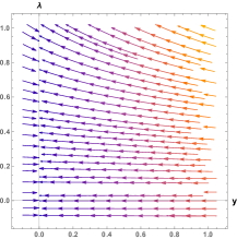
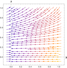
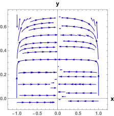
Figure 1: 2D phase portrait for the $x=1,-1$ and $xy$ planes and shows that even though the critical points are non-hyperbolic, one can still take some particular limits to see the matter dominated to de Sitter transition.

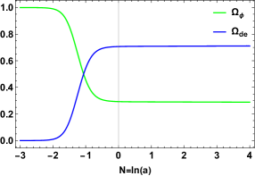
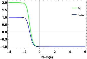
Figure 2: Evolutionary profile of scalar field density, dark energy density, deceleration, and the equation of state parameter for the exponential potential in DBI scalar field.

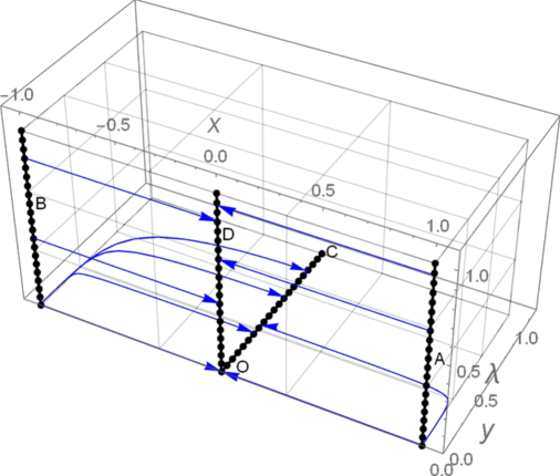
Figure 3: The 3-D phase-space trajectories plotted for a set of solutions to the autonomous system corresponding to the exponential potential.

Table 1: Table shows the critical points and their behaviour corresponding to the model $f(Q)=-Q+\alpha Q^{n}$ with potential $V(\phi)=V_{0}e^{-\beta\phi}$.

Critical Points $(x_{c},y_{c},z_{c})$	Eigenvalues ($\lambda_{1}$, $\lambda_{2}$, $\lambda_{3}$)	Nature of critical point	$q$	$\omega$
$O(0,0,0)$	$(-3,0,0)$	Stable	$-1$	$-1$
$A(1,0,\lambda)$	$(6,0,0)$	Non-hyperbolic	$-1$	$-1$
$B(-1,0,\lambda)$	$(6,0,0)$	Non-hyperbolic	$-1$	$-1$
$C(0,y,0)$	$(-3,0,0)$	Stable	$-1$	$-1$
$D(0,0,\lambda)$	$(-3,0,0)$	Stable	$-1$	$-1$

IV.3 Power-law potential

We assume the following form of power-law potential,

$$V(\phi)=V_{0}\phi^{-k}$$ (97)

For the polynomial potentials, we get the dynamical system equations as follows,
we get $\lambda=-\frac{V_{,\phi}}{V^{\frac{3}{2}}}=\frac{V_{0}k\phi^{-k-1}}{V_{0}\phi^{-k}(V_{0}\phi^{-k})^{\frac{1}{2}}}=\frac{k}{V_{0}^{\frac{1}{2}}}\phi^{-1+\frac{k}{2}}$
So we get

$$\lambda=\frac{k}{\sqrt{V_{0}}}\phi^{-1+\frac{k}{2}}$$

Also, for $k=2$ we get $\lambda=\frac{2}{\sqrt{V_{0}}}$.
We also note that $\Gamma=\frac{VV_{,\phi\phi}}{V_{,\phi}^{2}}=\frac{k+1}{K}$,
We also note that for $k=2$ $\Gamma=\frac{3}{2}$.
So the dynamical system of equations becomes,

$$x^{\prime}= (x^{2}-1)(3x-\sqrt{3}\lambda y)$$ (98)

$$y^{\prime}= -\frac{1}{2}y^{2}[\sqrt{3}\lambda xy+\frac{3x^{2}y}{[(n-1)\sqrt{1-x^{2}}-ny^{2}]}]$$ (99)

$$\lambda^{\prime}= \frac{\sqrt{3}(k-2)}{2k}xy\lambda^{2}$$ (100)

Solving the above ODE, we get the fixed points given below.

Table 2: Table shows the critical points and their behaviour corresponding to the model $f(Q)=-Q+\alpha Q^{n}$ with potential $V(\phi)=V_{0}\phi^{-k}$for $k\neq 2$.

Critical Points $(x_{c},y_{c},z_{c})$	Eigenvalues ($\lambda_{1}$, $\lambda_{2}$, $\lambda_{3}$)	Nature of critical point	$q$	$\omega$
$O^{\prime}(0,0,\lambda)$	$(-3,\sqrt{3}\lambda,0)$	Stable for $\lambda<0$ Non-hyperbolic for $\lambda\geq 0$	$-1$	$-1$
$A^{\prime}(x,y,0)$	$(-3,0,0)$	Stable	$-1$	$-1$
$B^{\prime}(0,y,0)$	$(-3,0,0)$	Stable	$-1$	$-1$

For $k=2$, we get the 2-dimensional dynamical system of the equation given as,

$$x^{\prime}= (x^{2}-1)(3x-\sqrt{3}\lambda y)$$ (101)

$$y^{\prime}= -\frac{1}{2}y^{2}[\sqrt{3}\lambda xy+\frac{3x^{2}y}{[(n-1)\sqrt{1-x^{2}}-ny^{2}]}]$$ (102)

For this, we get the fixed points in the following table.
We also note that from figure (4) the stable point is the de-Sitter type, which matches the previous analysis done by Copeland et al.[15].

Table 3: Table shows the critical points and their behaviour corresponding to the model $f(Q)=-Q+\alpha Q^{n}$ with potential $V(\phi)=V_{0}\phi^{-k}$for $k=2$(note that $\lambda^{\prime}=0$).

Critical Points $(x_{c},y_{c})$	Eigenvalues ($\lambda_{1}$, $\lambda_{2}$)	Nature of critical point	$q$	$\omega$
$O^{\prime\prime}(0,0)$	$(-3,\sqrt{3}\lambda)$	Stable for $\lambda<0$ Non-hyperbolic for $\lambda\geq 0$	$-1$	$-1$
$A^{\prime\prime}(x,y)$	$(-3,0)$	Stable	$-1$	$-1$
$B^{\prime\prime}(0,y)$	$(-3,0)$	Stable	$-1$	$-1$

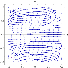
Figure 4: 2D phase portrait for polynomial potential when $k=2$

V Conclusion

In this article, we have studied the DBI scalar field and its effect on cosmology via dynamical system analysis. We note that such a lagrangian density is given by $\mathcal{L}_{Tachyon}=V(\phi)\sqrt{1+\partial\phi^{2}\partial^{\mu}\phi\partial_{\mu}\phi}$, and equating with Klein Gordon equation and finding the appropriate stress-energy tensor, we got the dynamical system equation for two different type of potential that is exponential and polynomial. Also, for the polynomial potential for a particular case $k=2$, we got a 2D dynamical system equation. We have analyzed all the dynamical system equations and plotted the 3D and 2D phase portraits.
In section IV, we begin with a non-linear $f(Q)$ functional, specifically $f(Q)=-Q+\Psi(Q)=-Q+\alpha Q^{n}$, where $\alpha$ and $n$ are free model parameters. The assumed functional form is a polynomial correction to the STEGR case and has great significance in early and late-time cosmology. The considered $f(Q)$ function with $n>1$ can potentially apply to the inflationary scenario, whereas the case $n<1$ corrects the late-time cosmology. Further, we have defined phase-space variables, and then we expressed the deceleration (68) and the effective equation of state parameter (39) in terms of phase-space variables. Now, to probe the cosmological implications of the considered scenario, we assumed two specific forms of the potential function, specifically the exponential one $V(\phi)=V_{0}e^{-\beta\phi}$ and the power-law $V(\phi)=V_{0}\phi^{-k}$ (and $V(\phi)=V_{0}\phi^{-2}$), which are widely discussed in the literature. The corresponding critical points and their behaviours for the obtained autonomous systems are presented in Table (1), (2) (and (3)).
First, we note that as both the polynomial and exponential potential give the same result (in terms of fixed point location and stability), it is enough to do for one. We also note that it is somewhat expected from the general theorem given by Hao et al. [21] and Chingangbam et al.[22] about the sufficient condition for a de-Sitter type solution. We can see from the fixed point list that our fixed points have a late time de-Sitter type solution, consistent with the general study [21, 22].
We also note that for exponential potential (for polynomial potential, the analysis is similar), we have explicitly calculated the necessary and sufficient condition for the fixed point $(\pm 1,0,\lambda)$ to show the transition from matter-dominated to de-Sitter type solutions. We also note that we have found that for general $n$ in $f(Q)$ gravity the necessary and sufficient condition for the fixed points $(\pm 1,0,\lambda)$ to show a matter-dominated phase to de-Sitter phase is given by $\frac{1-x}{y^{4}}\leq\frac{8}{(1-n)^{2}}$ (where in the limit $x\rightarrow 1$ and $y\rightarrow 0$). For the other fixed point $(-1,0,\lambda)$, one gets the similar bound over $x,y$ plane such that it gives matter to de-Sitter dominated solution. Figure (1) shows all the relevant 2D phase plots. We also note that among all the phase trajectories which reach $(\pm 1,0,\lambda)$, only the trajectory which satisfies the initial condition given above would be of interest as these trajectories show the transition to late time acceleration. In Figure (3) we have shown the 3D phase portrait of the full dynamical system and marked the fixed points. In Figure (2) we have shown how the phenomenological quantities in cosmology like $q,\omega,\Omega$ change with time, and we can see in late time $q,\omega\rightarrow-1$, which indicates the de-Sitter type solutions. We also note that in current time ($N=0$) $q\approx-0.8$ is somewhat consistent with the present observed value (-0.6). The discrepancy in $q$ comes as there is no dark matter or ordinary matter in our calculations.
We can see that the dynamical system equations are precisely similar for the polynomial case, so the fixed points and their classification (2) are identical. We have not repeated the analysis in this case. One notable exception is given for $k=2$, which gives $\lambda^{\prime}=0$, making it a two-2D autonomous system and the phase portrait is given in figure (4). This $k=2$ case has been studied in detail by [12, 15]. We also note that even for general $n$, the fixed points are consistent with the literature.
Throughout the present manuscript, we note that all the results have been developed for $\Psi(Q)=\alpha Q^{n}$ for arbitrary $\alpha$ and $n$; we also note that when $\alpha=0$ this reduced to pure GR case. Also, even though in literature there are many models of $f(Q)$ gravity are present, we note that beyond polynomial type modified gravity, the dynamical system is not autonomous (as it can be seen from (IV) calculations); hence the dynamical system analysis would not be possible. We have also tried other types of potentials for the DBI field, but there are no different potentials except for polynomial and exponential potentials. We have tried to close the dynamical system of equations. So, in a sense, we can say this is the most general dynamical system analysis for the DBI field in modified $f(Q)$ gravity as different forms of $f(Q)$ do not make the system autonomous, and different types of potentials does not close the dynamical system.

Data Availability

There are no new data associated with this article.

References

• [1] A.G. Riess et al., Astron. J. 116, 1009 (1998).
• [2] S. Perlmutter et al., ApJ 517, 565 (1999).
• [3] Green, Schwarz, Witten, Superstring Theory , Cambridge University Press (1988).
• [4] J. Polchinski, String Theory, Cambridge University Press (2005).
• [5] A. Mazumdar, S. Panda, and A. Perez-Lorenzana, Nuclear Physics B 614.1-2 101-116 (2001).
• [6] A. Sen, Modern Physics Letters A 17.27, 1797-1804 (2002).
• [7] A. Sen, JHEP 04, 048 (2002).
• [8] A. Sen, JHEP 07, 065 (2002).
• [9] T. Padmanabhan, Phys.Rev. D 66, 021301 (2002).
• [10] G. W. Gibbons, Phys. Lett. B 537, 1-4 (2002).
• [11] G. W. Gibbons, Class.Quant.Grav. 20, S321-S346 (2003).
• [12] J. Bhagla et al., Phys.Rev. D 67, 063504 (2003).
• [13] V. Gorini et al., Phys.Rev. D 69, 123512 (2004).
• [14] T. Padmanabhan et al., Phys.Rev. D 66, 081301 (2002).
• [15] E. J. Copeland et al., Phys.Rev. D 71, 043003 (2005).
• [16] Aguirregabiria et al.,Phys.Rev. D 69 , 123502 (2004).
• [17] W. Fang, H. Q. Lu, Eur. Phys. J C 68, 567-572 (2010).
• [18] Quiros et al., Class.Quant.Grav. 27, 215021 (2010).
• [19] Z. K. Guo et al., Phys.Rev. D 68, 043508 (2003).
• [20] E. Silverstein, D. Tong , Phys.Rev. D 70, 103505 (2004).
• [21] J. Hao, X. Li, Phys.Rev. D 68 , 083514 (2003).
• [22] P. Chingangbam , T. Qureshi, Int. J. Mod. Phys. A 20, 6083 (2005).
• [23] CANTATA collaboration, Modified Gravity and Cosmology: An Update by the CANTATA Network, arXiv, arXiv:2105.12582.
• [24] Timothy Clifton et al., Physics Reports 513, 1-189 (2012).
• [25] J. M. Nester and H.-J. Yo, Chin. J. Phys. 37, 113 (1999).
• [26] J.B. Jimenez, L. Heisenberg and T. Koivisto, Phys. Rev. D 98, 044048 (2018).
• [27] M. Hohmann et al, Phys. Rev. D 99, 024009 (2019).
• [28] F. D Ambrosio et al., Phys. Rev. D 105, 024042 (2022).
• [29] J. B. Jiménez et al., Phys. Rev. D 101, 103507(2020).
• [30] J.B. Jiménez, L. Heisenberg, and T. S. Koivisto, JCAP 08, 039 (2018).
• [31] F.K. Anagnostopoulos, S. Basilakos, and E. N. Saridakis, Phys. Lett. B, 822 (2021).
• [32] F. D’Ambrosio, L. Heisenberg, S. Kuhn, Class. Quantum Grav. 39, 025013 (2022).
• [33] S. Capozziello, V. De Falco, C. Ferrara, Eur. Phys. J. C. 82, 865 (2022).
• [34] D. Zhao, Eur. Phys. J. C 82, 303 (2022).
• [35] A. De and L.T. How, Phys. Rev. D, 106, 048501 (2022).
• [36] N. Frusciante, Phys. Rev. D 103, 0444021 (2021).
• [37] W. Khyllep, A. Paliathanasis and J. Dutta, Phys. Rev. D 103, 103521 (2021).
• [38] M. Calza and L. Sebastiani, Eur. Phys. J. C. 83, 247 (2023).
• [39] J. B. Jiménz, L. Heisenberg, and T. S. Koivisto, Universe 5, 173 (2019).
• [40] F. D’Ambrosio, L. Heisenberg, and S. Kuhn, Class. Quantum Grav. 39, 025013 (2021).
• [41] S. Bahamonde, C. G. Bohmer, S. Carloni, E. J. Copeland, W. Fang, and N. Tamanini, Phys. Rept. 775, 1-122 (2018).
• [42] J. B. Jiménez, L. Heisenberg, T. S. Koivisto, and S. Pekar, Phys. Rev. D 101, 103507 (2020).