Quasi-optimal Complexity $hp$-FEM

Quasi-optimal complexity $hp$-FEM for Poisson on a rectangle

Abstract

We show, in one dimension, that an $hp$-Finite Element Method ($hp$-FEM) discretisation can be solved in optimal complexity because the discretisation has a special sparsity structure that ensures that the reverse Cholesky factorisation—Cholesky starting from the bottom right instead of the top left—remains sparse. Moreover, computing and inverting the factorisation almost entirely trivially parallelises across the different elements. By incorporating this approach into an Alternating Direction Implicit (ADI) method à la Fortunato and Townsend (2020) we can solve, within a prescribed tolerance, an $hp$-FEM discretisation of the (screened) Poisson equation on a rectangle, in parallel, with quasi-optimal complexity: $O(N^{2}\log N)$ operations where $N$ is the maximal total degrees of freedom in each dimension. When combined with fast Legendre transforms we can also solve nonlinear time-evolution partial differential equations in a quasi-optimal complexity of $O(N^{2}\log^{2}N)$ operations, which we demonstrate on the (viscid) Burgers’ equation.

1 Introduction

Consider the classic problem of solving the (screened) Poisson equation in a rectangle:

(1) $$-\Delta u(x,y)+\omega^{2}u(x,y)=f(x,y)\quad\hbox{for}\quad a\leq x\leq b,\;c\leq y\leq d$$

where $\Delta u\coloneqq u_{xx}+u_{yy}$ is the Laplacian and we assume vanishing Dirichlet or Neumann boundary conditions. An effective and fast approach to solving this equation is the Fast Poisson Solver: using finite-differences to discretise the PDE, we can diagonalise the discretisation using the Discrete Cosine Transform in a way that leads to quasi-optimal complexity, that is, $O(N^{2}\log N)$ operations where $N$ is the maximal degrees of freedom along each dimension.

In this paper we introduce an alternative approach that also achieves quasi-optimal complexity but for a high order ($hp$) framework. We utilise the work of Babuška and Suri [4], which introduced a basis for the Finite Element Method (FEM) built from tensor products of piecewise integrated Legendre polynomials that achieved sparse discretisations for constant coefficient partial differential equations (PDEs) on rectangles. A fact that, perhaps, has been inadequately emphasised is that when combined with fast Legendre transforms [2, 26, 41], this approach enables quasi-optimal application of the discretisation: the complexity is $O(p^{2}n^{2}\log^{2}p)$ for a discretisation of a tensor product of $p$-degree polynomials where the rectangle is subdivided into $n^{2}$ rectangles (that is $h=1/n$ on the unit rectangle). Applying the discretisation quasi-optimally in an iterative framework is, therefore, a solved problem.

Inverting the discretisation is another story. While Fortunato and Townsend [18] introduced the first spectral Fast Poisson Solver, which achieves quasi-optimal complexity for solving the 2D Poisson equation with the aforementioned basis using the Alternating Direction Implicit (ADI) method, it only was applicable when there was a single element. The aim of this work is to extend their approach to an arbitrary number of elements in a manner that is robust to $h$- and $p$-refinement.

The ingredients that made [18] successful were:

1. a fast solve for one-dimensional discretisations.

2. control on the separation of the spectrum from the origin.

For (1) we introduce an optimal complexity $hp$-FEM solver in 1D in Section 4 for Symmetric Positive Definite (SPD) problems: the complexity is $O(pn)$ where $p$ is the polynomial degree and $n$ is the number of elements. For (2) we observe that the smallest eigenvalue can be computed in optimal complexity and we prove bounds built on known $hp$-FEM results that guarantee that it has the needed behaviour to achieve quasi-optimal complexity.

Sparse $p$- and $hp$-FEM have a rich history. They can be traced to the work of Szabó and Babuška [6], see also [39, Ch. 2.5.2] and [37, Ch. 3.1]. Extensions to two dimensions were further developed by Babuška and Suri [4] and Beuchler and Schöberl [10], where they construct a $p$-FEM on quadrilaterals and simplices, respectively. Other works of a similar theme include [5, 35, 8, 9, 24, 7, 17, 25, 37] and [38, App. A]. The focus of $hp$-FEM literature is often deriving the necessary frameworks, proving optimal mesh adaptivity strategies, and obtaining exponential convergence rates [37, 22].

The literature on fast solvers for the Poisson equation is extremely vast. To name but a few techniques: Fast Fourier Transforms (FFT), cyclic reductions [14], fast direct solvers for boundary element and multipole methods [33, 32], pseudospectral Fourier with polynomial subtraction [3, 11], the fast diagonalization method [30], multigrid methods [13, 20, 23, 29], and domain decomposition [21, 31]. Almost always there is a tradeoff between asymptotic complexity, speed, and flexibility of the methods, e.g. the structure required in the mesh. To our knowledge, except for the solver described in this work, there exists no fast Poisson solver in 2D that simultaneously (1) converges spectrally when the solution is smooth, (2) can mesh the domain into rectangular elements and, therefore, efficiently capture discontinuities in the data and (3) asymptotically requires only $O(N^{2}\log N)=O((pn)^{2}\log(pn))$ operations for the solve and $O(N^{2}\log^{2}N)=O((pn)^{2}\log^{2}(pn))$ operations for the setup.

The structure of the paper is as follows:

Section 2: we review the integrated Legendre functions of [4] (see also [37, Ch. 3.1.4]) and see how they lead to discretisations of differential operators with a very special sparsity structure which we call Banded-Block-Banded Arrowhead ($B^{3}$-Arrowhead) Matrices.

Section 3: we explain how the Poisson equation can be recast as a simple linear system involving a $B^{3}$-Arrowhead matrix in 1D and a Sylvester equation involving $B^{3}$-Arrowhead matrices in 2D.

Section 4: we show that a reverse Cholesky factorisation—a factorisation of a matrix as $A=L^{\top}L$ where $L$ is lower triangular— for $B^{3}$-Arrowhead matrices can be computed and the inverse applied in optimal complexity. Moreover, the factorisation naturally parallelises between different elements.

Section 5: we discuss the ADI method and how it can be used to solve the (screened) Poisson equation in quasi-optimal complexity. This requires spectral analysis of the underlying discretisations to control the number of iterations needed in ADI.

Section 6: we discuss how to transform between coefficients and values efficiently, using visicid Burgers equation in 2D with a discontinuous initial condition as an example.

Code availability: The numerical experiments found in this manuscript where conducted in Julia and and can be found at ADIPoisson.jl [27, 28].

2 Integrated Legendre functions

In this section we introduce the one-dimensional basis of integrated Legendre functions that underlies our discretisation of the Poisson equation.

2.1 A basis for a single interval

Define the weighted ultraspherical/Jacobi polynomials as

$$W_{k}(x)\coloneqq{(1-x^{2})C_{k}^{(3/2)}(x)\over(k+1)(k+2)}={(1-x^{2})P_{k}^{(1,1)}(x)\over 2(k+1)}$$

where $C_{k}^{(\lambda)}$ are orthogonal with respect to $(1-x^{2})^{\lambda-1/2}$ on $[-1,1]$ for $\lambda>-1/2$, $\lambda\neq 0$ with normalisation constant

$$C_{k}^{(\lambda)}(x)={2^{k}(\lambda)_{k}\over k!}x^{k}+O(x^{k-1})$$

where $(\lambda)_{k}=\lambda(\lambda+1)\cdots(\lambda+k-1)$ is the Pochammer symbol. $P_{k}^{(a,b)}(x)$ are Jacobi polynomials orthogonal with respect to $(1-x)^{a}(1+x)^{b}$ on $[-1,1]$ with normalisation constant given in [16, 18.3].

The choice of normalisation is chosen because it leads to the simple formula

(2) $$W_{k}^{\prime}(x)=-P_{k+1}(x)$$

for the Legendre polynomials $P_{k}(x)\equiv C_{k}^{(1/2)}(x)$ [16, 18.9.16]. In other words, they are the integral of Legendre polynomials: up to a constant they are precisely the integrated Legendre functions used by Babuška. They are also equivalent to the basis defined by Schwab [37, Ch. 3.1] and utilised by Fortunato and Townsend [18].

It is convenient to express this relationship in terms of quasi-matrices, which can be viewed as matrices that are continuous in the first dimension, or equivalently as a row-vector whose columns are functions:

$${{\rm d}\over{\rm d}x}\underbrace{[W_{0},W_{1},W_{2},\ldots]}_{\bf W}=\underbrace{[P_{0},P_{1},P_{2},\ldots]}_{\bf P}\underbrace{\begin{bmatrix}0\\ -1\\ &-1\\ &&-1\\ &&&\ddots\end{bmatrix}}_{D_{W}^{P}}.$$

If we have a single element in 1D we can use this basis as the test and trial basis in the weak formulation of a a differential equation. Let $\langle\cdot,\cdot\rangle$ denote the $L^{2}(-1,1)$-inner product. Then the Gram/mass matrix associated with Legendre polynomials is

$$\left\langle{{\bf P}^{\top},{\bf P}}\right\rangle\coloneqq\begin{bmatrix}\left\langle{P_{0},P_{0}}\right\rangle&\left\langle{P_{0},P_{1}}\right\rangle&\cdots\\ \left\langle{P_{1},P_{0}}\right\rangle&\left\langle{P_{1},P_{1}}\right\rangle&\cdots\\ \vdots&\vdots&\ddots\end{bmatrix}=\underbrace{\begin{bmatrix}2\\ &2/3\\ &&2/5\\ &&&\ddots\end{bmatrix}}_{M_{P}}$$

whilst the discretisation of the weak 1D Laplacian is diagonal:

$$-\Delta_{W} \coloneqq\left\langle{({\bf W}^{\prime})^{\top},{\bf W}^{\prime}}\right\rangle=\left\langle{({\bf P}D_{W}^{P})^{\top},{\bf P}D_{W}^{P}}\right\rangle$$

$$=(D_{W}^{P})^{\top}M_{P}D_{W}^{P}=\begin{bmatrix}2/3\\ &2/5\\ &&2/7\\ &&&\ddots\end{bmatrix}$$

which is another way to write the formula:

$$\langle W_{k}^{\prime},W_{j}^{\prime}\rangle=\langle P_{k+1},P_{j+1}\rangle={2\over 2k+3}\delta_{kj}.$$

The mass matrix can be deduced by using the lowering relationship:

(3) $$\underbrace{[W_{0},W_{1},W_{2},\ldots]}_{\bf W}=\underbrace{[P_{0},P_{1},P_{2},\ldots]}_{\bf P}\underbrace{\begin{bmatrix}\times\\ 0&\times\\ \times&0&\times\\ &\times&0&\times\\ &&\ddots&\ddots&\ddots\end{bmatrix}}_{L_{W}}$$

where the exact formulae for the entries is in Appendix A. For now we focus on sparsity structure. Subsequently the mass matrix can be expressed as a truncation of an infinite pentadiagonal matrix:

$$M_{W} \coloneqq\langle{\bf W}^{\top},{\bf W}\rangle=L_{W}^{\top}\langle{\bf P}^{\top},{\bf P}\rangle L_{W}=L_{W}^{\top}M_{P}L_{W}$$

$$=\begin{bmatrix}\times&0&\times\\ 0&\times&0&\times\\ \times&0&\times&0&\times\\ &\times&0&\times&0&\ddots\\ &&\times&0&\times&\ddots\\ &&&\ddots&\ddots&\ddots\end{bmatrix}.$$

The entries have simple explicit rational expressions, or alternatively one can view this as a product of banded matrices. The latter approach is slightly less efficient but we will use it for clarity in exposition. We can similarly find the matrix of the inner products that arise in testing with this basis:

$$\left\langle{{\bf W}^{\top},{\bf P}}\right\rangle=L_{W}^{\top}\left\langle{{\bf P}^{\top},{\bf P}}\right\rangle=L_{W}^{\top}M_{P}.$$

2.2 Multiple intervals

Partitioning an interval $[a,b]$ into $n$ subintervals $a=x_{0}<x_{1}<\cdots<x_{n}=b$ we can use an affine map

$$a_{j}(x)={2x-x_{j-1}-x_{j}\over x_{j}-x_{j-1}}$$

to the reference interval $[-1,1]$ to construct mapped bubble functions as

$$W_{kj}^{\bf x}(x)\coloneqq\begin{cases}W_{k}(a_{j}(x))&x\in[x_{j-1},x_{j}]\\ 0&\hbox{otherwise}\end{cases}$$

on each interval. We combine these with the standard piecewise linear hat basis

$$h_{0}^{\bf x}(x) \coloneqq\begin{cases}{x_{1}-x\over x_{1}-x_{0}}&x\in[x_{0},x_{1}],\\ 0&\hbox{otherwise},\end{cases}\;\;\;h_{n}^{\bf x}(x)\coloneqq\begin{cases}{x-x_{n-1}\over x_{n}-x_{n-1}}&x\in[x_{0},x_{1}],\\ 0&\hbox{otherwise},\end{cases}$$

$$h_{j}^{\bf x}(x) \coloneqq\begin{cases}{x-x_{j-1}\over x_{j}-x_{j-1}}&x\in[x_{j-1},x_{j}],\\ {x_{j+1}-x\over x_{j+1}-x_{j}}&x\in[x_{j},x_{j+1}],\\ 0&\hbox{otherwise},\end{cases}\qquad\hbox{for}\qquad j=1,\ldots,n-1.$$

The hat and bubble functions are sometimes known as the internal and external shape functions, respectively [37, Def. 3.4]. We form a block quasi-matrix by grouping together the hat functions and bubble functions of the same degree:

$${\bf C}^{\bf x}\coloneqq[\underbrace{h_{0}^{\bf x},\ldots,h_{n}^{\bf x}}_{{\bf H}^{\bf x}}|\underbrace{W_{01}^{\bf x},\ldots,W_{0n}^{\bf x}}_{{\bf W}_{0}^{\bf x}}|\underbrace{W_{11}^{\bf x},\ldots,W_{1n}^{\bf x}}_{{\bf W}_{1}^{\bf x}}|\cdots].$$

We relate this to the piecewise Legendre basis

$${\bf P}^{\bf x}\coloneqq[\underbrace{P_{01}^{\bf x},\ldots,P_{n1}^{\bf x}}_{{\bf P}_{1}^{\bf x}}|\underbrace{P_{02}^{\bf x},\ldots,P_{n2}^{\bf x}}_{{\bf P}_{2}^{\bf x}}|\cdots]$$

where

$$P_{kj}^{\bf x}(x)\coloneqq\begin{cases}P_{k}(a_{j}(x))&x\in[x_{j-1},x_{j}]\\ 0&\hbox{otherwise}\end{cases}.$$

In what follows we often omit the dependence on ${\bf x}$.

2.2.1 The mass matrix

Restricting to each panel, our basis is equivalent to a mapped version of the one panel basis defined above, hence we can re-expand ${\bf C}^{\bf x}$ in terms of ${\bf P}^{\bf x}$. First note that the mass matrix is diagonal, which we write in block form as:

$$\left\langle{({\bf P}^{\bf x})^{\top},{\bf P}^{\bf x}}\right\rangle=\underbrace{\left[\begin{array}[]{c | c|c |c }M_{11}&&\\ \hline\cr&M_{22}&\\ \hline\cr&&M_{33}\\ \hline\cr&&&\ddots\end{array}\right]}_{M_{P}^{\bf x}},$$

where $\langle\cdot,\cdot\rangle$ denotes the $L^{2}(a,b)$-inner product. Since piecewise Legendre polynomials completely decouple we can view this matrix as a direct sum:

$$M_{P}^{\bf x}=\left({{x_{1}-x_{0}\over 2}M_{P}}\right)\oplus\cdots\oplus\left({{x_{n}-x_{n-1}\over 2}M_{P}}\right)$$

where the direct sum corresponds to interlacing the entries of the matrix, i.e.,

$${\bf e}_{\ell}^{\top}M_{kj}{\bf e}_{\ell}={\bf e}_{k}^{\top}\left({{x_{\ell}-x_{\ell-1}\over 2}M_{P}}\right){\bf e}_{j}.$$

Note that given a piecewise polynomial $f$, its coefficients in the basis ${\bf P}^{\bf x}$ can be expressed as:

$$(M_{P}^{\bf x})^{-1}\left\langle{{\bf P}^{\bf x},f}\right\rangle.$$

We use this to determine the (block) connection matrix

$${\bf C}={\bf P}\underbrace{\left[\begin{array}[]{c | c|c |c | c}R_{00}&R_{01}&&\\ \hline\cr R_{10}&{\bf 0}&R_{12}&\\ \hline\cr&R_{21}&{\bf 0}&R_{23}\\ \hline\cr&&\ddots&\ddots&\ddots\end{array}\right]}_{R_{C}^{\bf x}}$$

where the blocks are

(4) $$R_{k0} \coloneqq M_{kk}^{-1}\left\langle{{\bf P}_{k}^{\top},{\bf H}}\right\rangle=\begin{bmatrix}\times&\times\\ &\ddots&\ddots\\ &&\times&\times\end{bmatrix}\in{\mathbb{R}}^{n\times(n+1)},$$

(5) $$R_{kj} \coloneqq M_{kk}^{-1}\left\langle{{\bf P}_{k}^{\top},{\bf W}_{j-1}}\right\rangle=\begin{bmatrix}\times&\\ &\ddots\\ &&\times\end{bmatrix}\in{\mathbb{R}}^{n\times n},\quad\hbox{for}\quad j>0,$$

with the explicit formulae for the entries given in Appendix A. We thus have the mass matrix

$$M_{C}^{\bf x} \coloneqq\left\langle{{\bf C}^{\top},{\bf C}}\right\rangle=R_{C}^{\top}M_{P}R_{C}$$

$$=\left[\begin{array}[]{c c c c | c c c | c c c | c c c | c c c}\times&\times&&&\times&&&\times&&&&&\\ \times&\times&\ddots&&\times&\ddots&&\times&\ddots&&&&\\ &\ddots&\ddots&\times&&\ddots&\times&&\ddots&\times&&&\\ &&\times&\times&&&\times&&&\times&&&\\ \hline\cr\times&\times&&&\times&&&&&&\times&&\\ &\ddots&\ddots&&&\ddots&&&&&&\ddots&\\ &&\times&\times&&&\times&&&&&&\times\\ \hline\cr\times&\times&&&&&&\times&&&&&&&&\\ &\ddots&\ddots&&&&&&\ddots&&&&&&\ddots&\\ &&\times&\times&&&&&&\times&&&&&&\\ \hline\cr&&&&\times&&&&&&\times&&&&&\\ &&&&&\ddots&&&&&&\ddots&&&\ddots&\\ &&&&&&\times&&&&&&\times&&&\\ \hline\cr&&&&&&&&&&&&&&&\\ &&&&&&&&\ddots&&&\ddots&&&\ddots&\\ &&&&&&&&&&&&&&&\\ \end{array}\right].$$

where again the entries have simple rational expressions that can be deduced from the components. The structure is important here: every block is banded, and every block not in the first row/column are diagonal.

2.2.2 The weak Laplacian

Similarly, we can express differentiation as a block-diagonal matrix:

$${{\rm d}\over{\rm d}x}{\bf C}={\bf P}\underbrace{\left[\begin{array}[]{c | c|c }D_{00}&&\\ \hline\cr&D_{11}&\\ \hline\cr&&\ddots\end{array}\right]}_{D^{\bf x}},$$

where the blocks are

(6) $$D_{00} \coloneqq M_{{\bf P}_{0}}^{-1}\left\langle{{\bf P}_{0}^{\top},{\bf H}^{\prime}}\right\rangle=\begin{bmatrix}\times&\times\\ &\ddots&\ddots\\ &&\times&\times\end{bmatrix}\in{\mathbb{R}}^{n\times(n+1)},$$

(7) $$D_{kj} \coloneqq M_{{\bf P}_{k}}^{-1}\left\langle{{\bf P}_{k}^{\top},{\bf W}_{j-1}^{\prime}}\right\rangle=\begin{bmatrix}\times&\\ &\ddots\\ &&\times\end{bmatrix}\in{\mathbb{R}}^{n\times n},\quad\hbox{for}\quad j>0,$$

with the explicit entries given in Appendix A. We thus deduce that the weak Laplacian is also block diagonal with structure

$$-\Delta_{C}^{\bf x} \coloneqq\left\langle{({\bf C}^{\prime})^{\top},{\bf C}^{\prime}}\right\rangle=(D)^{\top}M_{P}D$$

$$=\left[\begin{array}[]{c c c c | c c c | c c c }\times&\times&&&&&\\ \times&\times&\ddots&&&&\\ &\ddots&\ddots&\times&&&\\ &&\times&\times&&&\\ \hline\cr&&&&\times&&\\ &&&&&\ddots&\\ &&&&&&\times\\ \hline\cr&&&&&&&&&\\ &&&&&&&&\ddots&\\ &&&&&&&&&\end{array}\right].$$

Again the structure is important: we have a block diagonal matrix whose blocks are all diagonal, apart from the first which is still banded.

2.3 Homogeneous Dirichlet boundary condition

To enforce homogeneous Dirichlet boundary conditions we need to drop the basis functions that do not vanish at the boundary, that is, the first and last hat function. Thus we use the following basis:

$${{\bf Q}}^{\bf x} \coloneqq{\bf C}^{\bf x}\underbrace{\left[\begin{array}[]{c c c c | c c c | c c c }0&&&&&&\\ 1&&&&&&\\ &\ddots&&&&&\\ &&1&&&&\\ &&0&&&&\\ \hline\cr&&&&1&&\\ &&&&&\ddots&\\ &&&&&&1\\ \hline\cr&&&&&&&&&\\ &&&&&&&&\ddots&\\ &&&&&&&&&\end{array}\right]}_{P_{D,n}}$$

$$=[\underbrace{h_{1},\ldots,h_{n-1}}_{\tilde{\bf H}}|\underbrace{W_{01},\ldots,W_{n1}}_{{\bf W}_{1}}|\underbrace{W_{02},\ldots,W_{n2}}_{{\bf W}_{2}}|\cdots].$$

The discretised operators are the same as above but with the first and last row of the first row/column blocks removed which modifies the band structure, i.e. we have

$$M_{Q}^{\bf x} \coloneqq\left\langle{({\bf Q})^{\top},{\bf Q}}\right\rangle=P_{D}^{\top}M_{C}P_{D}$$

$$=\left[\begin{array}[]{c c c c | c c c | c c c | c c c | c c c}\times&\times&&&\times&&&\times&&&&&\\ \times&\times&\ddots&&\times&\ddots&&\times&\ddots&&&&\\ &\ddots&\ddots&\times&&\ddots&\times&&\ddots&\times&&&\\ &&\times&\times&&&\times&&&\times&&&\\ \hline\cr\times&\times&&&\times&&&&&&\times&&\\ &\ddots&\ddots&&&\ddots&&&&&&\ddots&\\ &&\times&\times&&&\times&&&&&&\times\\ \hline\cr\times&\times&&&&&&\times&&&&&&&&\\ &\ddots&\ddots&&&&&&\ddots&&&&&&\ddots&\\ &&\times&\times&&&&&&\times&&&&&&\\ \hline\cr&&&&\times&&&&&&\times&&&&&\\ &&&&&\ddots&&&&&&\ddots&&&\ddots&\\ &&&&&&\times&&&&&&\times&&&\\ \hline\cr&&&&&&&&&&&&&&&\\ &&&&&&&&\ddots&&&\ddots&&&\ddots&\\ &&&&&&&&&&&&&&&\\ \end{array}\right].$$

As before every block is banded, and every block not in the first row/column are diagonal. The primary difference with the ${\bf C}^{\bf x}$ case above is the bandwidths of some of the blocks.

3 Discretisations of the screened Poisson equation

In order to discuss the FEM discretisation of Eq. 1 we first recast it in variational form. Let $\Omega=[a,b]\times[c,d]$ and $H^{s}(\Omega)\coloneqq W^{s,2}(\Omega)$ where $W^{s,q}(\Omega)$, $s>0$, $q\geq 1$, denote the standard Sobolev spaces [1]. We use $L^{q}(\Omega)$, $q\geq 1$, to denote the Lebesgue spaces and the notation $H^{1}_{0}(\Omega)$ for the space $\{v\in H^{1}(\Omega):v|_{\partial\Omega}=0\}$ where $|_{\partial\Omega}:H^{1}(\Omega)\to H^{1/2}(\Omega)$ denotes the usual trace operator [19]. Let $H^{-1}(\Omega)=(H^{1}_{0}(\Omega))^{*}$ denote the dual space of $H^{1}_{0}(\Omega)$. Moreover, given a Banach space $X$ and Hilbert space $H$, then $\langle\cdot,\cdot\rangle_{X^{*},X}$ denotes the duality pairing between a function in $X$ and a functional in the dual space $X^{*}$, and $\langle\cdot,\cdot\rangle_{H}$ denotes the inner product in $H$. As in the previous section, we drop the subscript when utilising the $L^{2}(\Omega)$-inner product. Given an $f\in H^{-1}(\Omega)$, we may rewrite the Poisson equation in variational (weak) form as: find $u\in H^{1}_{0}(\Omega)$ that satisfies

(8) $$\langle\nabla v,\nabla u\rangle+\omega^{2}\langle v,u\rangle=\langle v,f\rangle_{H^{1}_{0}(\Omega),H^{-1}(\Omega)}\;\;\text{for all}\;\;v\in H^{1}_{0}(\Omega),$$

where $\nabla u=(u_{x},u_{y})^{\top}$ is the gradient operator. To construct a discretisation in the FEM framework one chooses subspaces of $H^{1}(\Omega)$ as trial space (discretisation of $u$) and test space (discretisation of $v$), specified by their bases, which are termed trial and test bases, respectively.

3.1 Screened Poisson in 1D

For zero Dirichlet problems we use as both the test and trial basis ${\bf Q}$ up to degree $p$:

$${\bf Q}_{0:p}\coloneqq{\bf Q}\underbrace{\begin{bmatrix}I_{n-1}\\ &I_{n}\\ &&\ddots\\ &&&I_{n}\\ &&&0_{n\times n}\\ &&&\vdots\end{bmatrix}}_{I_{0:p}\in{\mathbb{R}}^{\infty\times N}}=[\tilde{\bf H}|{\bf W}_{0}|\cdots|{\bf W}_{p-2}],$$

where $N=(p+1)n-1$ is the total degrees of freedom in our basis up to degree $p$. That is, we approximate the solution, for ${\bf u}_{p}\in{\mathbb{R}}^{N}$: $u(x)\approx u_{p}(x)\coloneqq{\bf Q}_{0:p}(x){\bf u}_{p}$ and represent our test functions as $v_{p}={\bf Q}_{0:p}{\bf v}_{p}$. The discretisation of our weak formulation then becomes:

$$\left\langle{v_{p}^{\prime},u_{p}^{\prime}}\right\rangle+\omega\left\langle{v_{p},u_{p}}\right\rangle\; ={\bf v}_{p}^{\top}\left\langle{(({\bf Q}_{0:p})^{\prime})^{\top},({\bf Q}_{0:p})^{\prime}}\right\rangle{\bf u}_{p}+\omega{\bf v}_{p}^{\top}\left\langle{({\bf Q}_{0:p})^{\top},({\bf Q}_{0:p})^{\prime}}\right\rangle{\bf u}_{p}$$

$$={\bf v}_{p}^{\top}(-\underbrace{I_{0:p}^{\top}\Delta_{Q}I_{0:p}}_{\Delta_{Q,p}}+\omega^{2}\underbrace{I_{0:p}^{\top}M_{Q}I_{0:p}}_{M_{Q,p}}){\bf u}_{p}.$$

If we further assume that we have made a piecewise polynomial approximation of our right-hand side as $f\approx f_{p}\coloneqq{\bf P}_{0:p}{\bf u}_{p}$, computed via a fast Legendre transform ([41] or otherwise), the right-hand side becomes:

$$\left\langle{v_{p},f}\right\rangle\; ={\bf v}_{p}^{\top}I_{0:p}^{\top}\left\langle{{\bf Q}^{\top},{\bf P}}\right\rangle I_{0:p}{\bf f}_{p}={\bf v}_{p}^{\top}I_{0:p}^{\top}R_{Q}^{\top}\left\langle{{\bf P}^{\top},{\bf P}}\right\rangle I_{0:p}{\bf f}_{p}$$

$$={\bf v}_{p}^{\top}\underbrace{I_{0:p}^{\top}R_{Q}^{\top}I_{0:p}}_{R_{Q,p}^{\top}}\underbrace{I_{0:p}^{\top}M_{P}I_{0:p}}_{M_{P,p}}{\bf f}_{p}.$$

Enforcing this equation for all ${\bf v}_{p}\in{\mathbb{R}}^{N}$ leads us to an $N\times N$ system of equations:

$$(-\Delta_{Q,p}+\omega^{2}M_{Q,p}){\bf u}_{p}=R_{Q,p}^{\top}M_{P,p}{\bf f}_{p}.$$

3.2 Screened Poisson in 2D

For 2D problems we consider partitions $a=x_{1}<\cdots<x_{m}=b$ and $c=y_{1}<\cdots<y_{n}=d$ with truncation up to degrees $p$ and $q$, respectively. Then our basis for zero Dirichlet problems is given by the tensor product of ${\bf Q}^{\bf x}$ and ${\bf Q}^{\bf y}$, more specifically we have

$$u(x,y)\approx u_{pq}(x,y)\coloneqq{\bf Q}_{0:p}^{\bf x}(x)U_{pq}{\bf Q}_{0:q}^{\bf y}(y)^{\top}$$

where we represent the unknown coefficients as a matrix $U_{pq}\in{\mathbb{R}}^{M\times N}$ for $M=(p+1)m-1$ and $N=(q+1)n-1$. Similarly we may express the right-hand side as

$$f(x,y)\approx f_{pq}(x,y)={\bf P}_{0:p}^{\bf x}(x)F_{pq}{\bf P}_{0:q}^{\bf y}(y)^{\top}.$$

Consider an arbitrary test function $v_{pq}(x,y)={\bf Q}_{0:p}^{\bf x}(x)V_{pq}{\bf Q}_{0:q}^{\bf y}(y)$. By substituting in the expressions for $u$, $v$ and $f$ into Eq. 8, then akin to the 1D case, we arrive at

$$(-\Delta_{Q,p}^{\bf x})U_{pq}M_{Q,q}^{\bf y} +M_{Q,p}^{\bf x}U_{pq}(-\Delta_{Q,q}^{\bf y})+\omega^{2}M_{Q,p}^{\bf x}U_{pq}M_{Q,q}^{\bf y}$$

$$=(R_{Q,p}^{\bf x})^{\top}M_{P,p}^{\bf x}F_{pq}M_{P,q}^{\bf y}R_{Q,q}^{\bf y}.$$

We can modify this into a Sylvester’s equation:

$$(-\Delta_{Q,p}^{\bf x}+{\omega^{2}\over 2}M_{Q,p}^{\bf x})U_{pq}M_{Q,q}^{\bf y} +M_{Q,p}^{\bf x}U_{pq}(-\Delta_{Q,q}^{\bf y}+{\omega^{2}\over 2}M_{Q,q}^{\bf y})$$

(9) $$=(R_{Q,p}^{\bf x})^{\top}M_{P,p}^{\bf x}F_{pq}M_{P,q}^{\bf y}R_{Q,q}^{\bf y}.$$

In Section 5 we will discuss how to solve Eq. 9 for $U_{pq}$ in quasi-optimal complexity.

3.3 Neumann boundary conditions

If we do not impose vanishing conditions at the endpoints, that is, we use the full basis ${\bf C}^{\bf x}$ in weak form, it imposes natural boundary conditions, that is, a zero Neumann boundary condition. Everything else is the same as above with ${\bf C}^{\bf x}$ in-place of ${\bf Q}^{\bf x}$: the choice of basis is dictating the boundary conditions. It is also possible to use mixed Dirichlet–Neumann boundary conditions by modifying the basis; i.e., including $h_{0}^{\bf x}$ but not $h_{n}^{\bf x}$ imposes Neumann boundary conditions on the left but Dirichlet boundary conditions on the right.

4 Optimal complexity Cholesky factorisation

As noted, the mass matrices $M_{C}$/$M_{Q}$ and weak Laplacians $\Delta_{C}$/$\Delta_{Q}$ have a special sparsity structure:

Definition 4.1.

A Banded-Block-Banded-Arrowhead ($B^{3}$-Arrowhead) Matrix $A\in{\mathbb{R}}^{m+pn\times m+pn}$ with block-bandwidths $(\ell,u)$ and sub-block-bandwidth $\lambda+\mu$ has the following properties:

1. It is a block-banded matrix with block-bandwidths $(\ell,u)$.

2. The top-left block $A_{0}\in{\mathbb{R}}^{m\times m}$ is banded with bandwidths $(\lambda+\mu,\lambda+\mu)$.

3. The remaining blocks in the first row $B_{k}\in{\mathbb{R}}^{m\times n}$ have bandwidths $(\lambda,\mu)$.

4. The remaining blocks in the first column $C_{k}\in{\mathbb{R}}^{n\times m}$ have bandwidths $(\mu,\lambda)$.

5. All other blocks $D_{k,j}\in{\mathbb{R}}^{n\times n}$ are diagonal.

We represent the matrix in block form

(17) $$\begin{bmatrix}A_{0}&B\\ C&D\end{bmatrix}=\left[\begin{array}[]{c|c|c|c|c|c|c}A_{0}&B_{1}&\cdots&B_{u}&&\\ \hline\cr C_{1}&D_{1,1}&\cdots&D_{1,u}&D_{1,1+u}&\\ \hline\cr\vdots&\vdots&\ddots&\ddots&\ddots&\ddots\\ \hline\cr C_{l}&D_{\ell,1}&\ddots&\ddots&\ddots&\ddots&D_{p-u,p}\\ \hline\cr&D_{\ell+1,1}&\ddots&\ddots&\ddots&\ddots&D_{p-u+1,p}\\ \hline\cr&&\ddots&\ddots&\ddots&\ddots&\vdots\\ \hline\cr&&&D_{p,p-\ell}&D_{p,p-\ell+1}&\cdots&D_{p,p}\end{array}\right]$$

where $A_{0},B_{1},\ldots,B_{u},C_{1},\ldots,C_{\ell}$ are all banded matrices with bandwidths $(\lambda,\mu)$ whilst $D_{k,j}$ are diagonal matrices. To store the diagonal blocks in $D$ we write

$$D=D_{1}\oplus\cdots\oplus D_{n}$$

where $D_{k}$ are banded matrices with bandwidths $(\ell,u)$, where as above the direct sum corresponds to interlacing the entries of the matrix.

If we apply a Cholesky factorisation $A=LL^{\top}$ directly we will have fill-in coming from the banded initial rows/columns. The key observation is that if we use a reverse Cholesky factorisation, that is a factorisation of the form $A=L^{\top}L$ which begins in the bottom right, we avoid fill-in.

Theorem 4.2.

If $A$ is a Symmetric Positive Definite (SPD) $B^{3}$-Arrowhead Matrix which has block-bandwidth $(\ell,\ell)$ and sub-block-bandwidth $\lambda+\mu$ then it has a reverse Cholesky factorisation

$$A=L^{\top}L$$

where $L$ is a $B^{3}$-Arrowhead Matrix with block-bandwidth $(\ell,0)$ and sub-block-bandwidth $\lambda+\mu$.

Proof 4.3.

We begin by writing $A$ as a block matrix:

$$A=\begin{bmatrix}A_{0}&B\\ B^{\top}&D\end{bmatrix},$$

where

$$D=D_{1}\oplus\cdots\oplus D_{n}.$$

The reverse Cholesky factorisation $D=\tilde{L}^{\top}\tilde{L}$ can be deduced from the reverse Cholesky factorisations of $D_{j}=L_{j}^{\top}L_{j}$. In particular we have that

$$\tilde{L}\coloneqq L_{1}\oplus\cdots\oplus L_{n}\qquad\hbox{and}\qquad\tilde{L}^{-1}=L_{1}^{-1}\oplus\cdots\oplus L_{n}^{-1}.$$

Now write

$$A=\begin{bmatrix}A_{0}&B\\ B^{\top}&\tilde{L}^{\top}\tilde{L}\end{bmatrix}=\begin{bmatrix}I&B\tilde{L}^{-1}\\ &\tilde{L}^{\top}\end{bmatrix}\begin{bmatrix}A_{0}-B\tilde{L}^{-1}\tilde{L}^{-\top}B^{\top}&\\ &I\end{bmatrix}\begin{bmatrix}I\\ \tilde{L}^{-\top}B^{\top}&\tilde{L}\end{bmatrix}.$$

Write $\tilde{L}^{-1}$ in block form

$$\tilde{L}^{-1}=\left[\begin{array}[]{c | c | c}\tilde{L}_{1,1}&&\\ \hline\cr\vdots&\ddots\\ \hline\cr\tilde{L}_{p,1}&\cdots&\tilde{L}_{p,p}\end{array}\right]$$

noting each block is diagonal. We see that

$$B\tilde{L}^{-1}=[B_{1}\tilde{L}_{1,1}+\cdots+B_{\ell}\tilde{L}_{\ell,1}|B_{2}\tilde{L}_{2,2}+\cdots+B_{\ell}\tilde{L}_{\ell,2}|\cdots|B_{\ell}\tilde{L}_{\ell,\ell}|0|\cdots|0]$$

where each block has bandwidth $(\lambda,\mu)$. Thus

$$B\tilde{L}^{-1}\tilde{L}^{-\top}B^{\top}=(B_{1}\tilde{L}_{1,1}+\cdots+B_{\ell}\tilde{L}_{\ell,1})(\tilde{L}_{1,1}B_{1}^{\top}+\cdots+\tilde{L}_{\ell,1}B_{\ell}^{\top})+\cdots+B_{\ell}\tilde{L}_{\ell,\ell}^{2}B_{\ell}^{\top}$$

has bandwidths $(\lambda+\mu,\lambda+\mu)$, as multiplying banded matrices adds the bandwidths. Thus $A_{0}-BL^{-1}L^{-\top}B^{\top}=L_{0}^{\top}L_{0}$ also has bandwidths $(\lambda+\mu,\lambda+\mu)$ and its reverse Cholesky factor has bandwidth $(\lambda+\mu,0)$. Thus

$$L=\begin{bmatrix}L_{0}\\ \tilde{L}^{-\top}B^{\top}&\tilde{L}\end{bmatrix}$$

is a lower triangular $B^{3}$-Arrowhead matrix with the prescribed sparsity.

Encoded in this proof is a simple algorithm for computing the reverse Cholesky factorisation, see Algorithm 1.

Algorithm 1 Reverse Cholesky for $B^{3}$-Arrowhead Matrices

Input: Symmetric positive definite $B^{3}$-Arrowhead Matrix $A$ with block-bandwidths $(\ell,\ell)$ and sub-block-bandwidths $(\lambda,\lambda)$.

Output: Lower triangular $B^{3}$-Arrowhead Matrix with block-bandwidths $(\ell,0)$ and sub-block-bandwidths $(\lambda,\lambda)$ satisfying $A=L^{\top}L$.

1:  for $k=1,\ldots,n$ do

2:     Compute the banded reverse Cholesky factorisations $D_{k}=L_{k}^{\top}L_{k}$.

3:  end for

4:  for $k=1,\ldots,\ell$ do

5:     Construct banded matrices

$$M_{k}=B_{k}\tilde{L}_{k,k}+\cdots+B_{\ell}\tilde{L}_{\ell,k}.$$

6:  end for

7:  Form the banded matrix

$$\tilde{A}_{0}=M_{1}M_{1}^{\top}+\cdots+M_{\ell}M_{\ell}^{\top}.$$

8:  Compute the banded reverse Cholesky factorisation $\tilde{A}_{0}=L_{0}^{\top}L_{0}$.

9:  Return the lower triangular $B^{3}$-Arrowhead matrix

$$\begin{bmatrix}L_{0}\\ C&L_{1}\oplus\cdots\oplus L_{n}\end{bmatrix}$$

where $C^{\top}=[M_{1}|\cdots|M_{\ell}|0|\cdots|0]$.

Corollary 4.4.

If $A\in{\mathbb{R}}^{N\times N}$ is an SPD $B^{3}$-Arrowhead Matrix then the reverse Cholesky factorisation can be computed and its inverse applied in optimal complexity ($O(N)$ operations).

Proof 4.5.

The reverse Cholesky factorisations of banded matrices can be computed in optimal complexity so lines (1–3) take $O(np)$ operations. Multiplying banded matrices by diagonal matrices and adding them is also optimal complexity hence lines (4–7) take $O(\max(n,m))$ operations. Finally line (8) is another banded reverse Cholesky which is $O(m)$ operations. Hence the total complexity of the reverse Cholesky factorisation is $O(np+\max(n,m))=O(N)$ operations.

Once the factorisation is computed it is straightforward to solve linear systems in optimal complexity: write

$$L=\begin{bmatrix}L_{0}\\ L_{1}&\tilde{L}\end{bmatrix}\quad\hbox{so that}\quad L^{-1}=\begin{bmatrix}L_{0}^{-1}\\ -\tilde{L}^{-1}L_{1}L_{0}^{-1}&\tilde{L}^{-1}\end{bmatrix}.$$

Since $L_{0}$ is banded and $\tilde{L}=L_{1}\oplus\cdots\oplus L_{n}$ where $L_{k}$ are banded, their inverses can be applied in optimal complexity.

In Figure 1 we demonstrate the timing for this algorithm for solving the one-dimensional screened Poisson equation

$$(-\Delta+\omega^{2})u=f$$

with a zero Dirichlet boundary condition which is discretised via

$$(-\Delta_{Q}+\omega^{2}M_{Q})u=R^{\top}M_{P}\bf f$$

where $\bf f$ are given Legendre coefficients. We choose $\omega=1$ and $f$ is random samples as these do not impact the speed of the simulation. The first plot shows the precomputation cost: building the discretisation and computing its Cholesky factorisation, achieving optimal complexity. The second plot shows the solve time, which is also optimal complexity. The timings of both are roughly independent of $n$, the number of elements, demonstrating uniform computational cost.

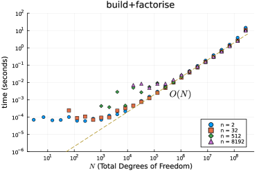
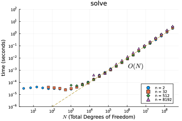
Figure 1: Time taken to build/factorise and solve a discretisation of a 1D (screened) Poisson equation up to degree $p$, where $n$ is the number of elements. The $x$-axis is $N=np-1$, the total number of degrees of freedom and demonstrates that the complexity is optimal as either $n\ (=2/h)$ or $p$ become large, and largely only depends on the total number of degrees of freedom.

Remark 4.6.

An $O(N)$ solve for the matrix induced by the FEM discretisation of the one-dimensional screened Poisson equation is also admissible via static condensation [37, Ch. 3.2].

Figure 2: Time taken to factorise and solve a 1D (screened) Poisson equation up to degree $p$, where $n=8$ is the number of elements, where we parallelise over multiple cores, on an M2 MacBook Air with 4 high performance and 4 high efficiency cores, using shared memory. We see substantial speedup when utilising the 4 high performance cores whilst a marginal speedup when also using the high efficiency cores.

5 A generalised Alternating Direction Implicit (ADI) method

Recall from Section 3.2, the generalised Sylvester equation for the two-dimensional screened Poisson equation (dropping the superscripts ^x and ^y) is

(18) $$\begin{split}\left(-\Delta_{Y,p}+\frac{\omega^{2}}{2}M_{Y,p}\right)U_{pp}M_{Y,p}&+M_{Y,p}U_{pp}\left(-\Delta_{Y,p}+\frac{\omega^{2}}{2}M_{Y,p}\right)\\ &=R_{Y,p}^{\top}M_{P,p}F_{pp}M_{P,p}R_{Y,p}\eqqcolon G_{pp}.\end{split}$$

Here ${\bf Y}_{0:p}(x)={\bf C}_{0:p}(x)$ if we consider the screened Poisson equation with a zero Neumann boundary condition and $\omega^{2}>0$. Otherwise ${\bf Y}_{0:p}(x)={\bf Q}_{0:p}(x)$ if we impose a zero Dirichlet boundary condition and $\omega^{2}\geq 0$.

We will solve (18) using a variant of the Alternating Direction Implicit (ADI) method. ADI is an iterative approach to approximate $X$ that solves the Sylvester equation $AX-XB=F$, but in a manner that permits precise error control: given two assumptions on real-valued matrices $A$ and $B$, one is able to explicitly find the number of iterations required for the algorithm to compute $X$ up to a maximum tolerance $\epsilon$. The two assumptions are [18]:

1. $A$ and $B$ are symmetric matrices;

2. There exist real disjoint nonempty intervals $[a,b]$ and $[c,d]$ such that $\sigma(A)\subset[a,b]$ and $\sigma(B)\subset[c,d]$, where $\sigma$ denotes the spectrum of a matrix.

Algorithm 2 Generalised Alternating Direction Implicit (ADI)

Input: Symmetric matrices $A\in{\mathbb{R}}^{M\times M}$, $B\in{\mathbb{R}}^{N\times N}$, $C\in{\mathbb{R}}^{M\times M}$, and $D\in{\mathbb{R}}^{M\times N}$, matrix $F\in{\mathbb{R}}^{M\times N}$, tolerance $\epsilon$.

Output: Matrix $U\in{\mathbb{R}}^{M\times N}$ satisfying $AUD-CUB\approx F$.

Precomputation:

1:  Use the banded symmetric generalised eigenvalue algorithms [15] to compute generalised eigenvalues $\sigma(A,C)$ and $\sigma(B,D)$. The largest and smallest eigenvalues give us $a,b,c,d$ such that $\sigma(\tilde{A})\subset[a,b]$ and $\sigma(\tilde{B})\subset[c,d]$.

2:  Let the number of iterations equal $J=\lceil\log(16\gamma)\log(4/\epsilon)/\pi^{2}\rceil$ where $\gamma=|c-a||d-b|/(|c-b||d-a|)$.

3:  Compute The ADI shifts $p_{j}$ and $q_{j}$ have explicit formulae depending on $\gamma$ [18, Eq. (2.4)]. Notably, we have that $p_{j}>0$ and $q_{j}<0$ for all $j\in\{1,\ldots,J\}$.

4:  for $j=1,\ldots,J$ do

5:     Compute the reverse Cholesky factorisations of $q_{j}A-C$ and $p_{j}B-D$.

6:  end for

Solve:

1:  Let $W_{0}={\bf 0}$

2:  for $j=1,\ldots,J$ do

3:     Use the precomputed Cholesky factorisations to compute

$$W_{j-1/2} =((A-p_{j}C)W_{j-1}-F)(B-p_{j}D)^{-1},$$

$$W_{j} =(A-q_{j}C)^{-1}(W_{j}(B-q_{j}D)-F).$$

4:  end for

5:  return  $W_{J}C^{-1}$.

The algorithm proceeds iteratively. First one fixes the initial matrix $X_{0}=0$. Then, iteratively for $j=1,\dots,J$, we compute

(19) for $$X_{j-1/2} X_{j-1/2}(B-p_{j}I) =F-(A-p_{j}I)X_{j-1},$$ solve

(20) for $$X_{j} (A-q_{j}I)X_{j} =F-X_{j-1/2}(B-q_{j}I).$$ solve

5.1 Generalised ADI

In the case of the 2D (Screened) Poisson equation (8) we have a generalised Sylvester equation which we write in general form as:

$$AUC-DUB=F.$$

We first extend the ADI method to generalised problems in Algorithm 2.

Lemma 5.1.

Write $C=L^{\top}L$ and $D=V^{\top}V$ where $L$ and $V$ are lower triangular. Algorithm 2 computes $U_{J}$ satisfying

$$\left\|V(U-U_{J})L^{\top}\right\|\leq\epsilon\left\|VUL^{\top}\right\|.$$

Proof 5.2.

We reduce a generalised Sylvester equation to a standard Sylvester equation as follows: write $D=V^{\top}V$ where $V$ is lower triangular we define $X\coloneqq VUL^{\top}$ so that our equation becomes

$$\underbrace{V^{-\top}AV^{-1}}_{\tilde{A}}X-X\underbrace{L^{-\top}BL^{-1}}_{\tilde{B}}=\underbrace{V^{-\top}FL^{-1}}_{G}.$$

$\tilde{A}$ and $\tilde{B}$ are symmetric matrices whose eigenvalues satisfy $\sigma(\tilde{A})=\sigma(A,C)$ and $\sigma(\tilde{B})=\sigma(B,D)$. The ADI iterations satisfy, for $X_{0}=0$,

$$X_{j-1/2}(\tilde{B}-p_{j}I) =G-(\tilde{A}-p_{j}I)X_{j-1},$$

$$(\tilde{A}-q_{j}I)X_{j} =G-X_{j-1/2}(\tilde{B}-q_{j}I),$$

where by convergence of the ADI algorithm [18, Th. 2.1]:

(21) $$\|X-X_{J}\|\leq\epsilon\|X\|.$$

Writing $W_{j}\coloneqq V^{-1}X_{j}L$ and $W_{j+1/2}\coloneqq V^{\top}X_{j+1/2}L^{-\top}$ this iteration becomes equivalent to that of Algorithm 2. We thus have, for $U_{J}=W_{J}C^{-1}=V^{-1}X_{J}L^{-\top}$, that

$$\left\|V(U-U_{J})L^{\top}\right\|=\left\|X-X_{J}\right\|\leq\epsilon\left\|X\right\|=\epsilon\left\|VUL^{\top}\right\|.$$

In Figure 3 we show the solution for a discontinuous-right hand side using ADI with a fixed $h$ and high $p$ to compute the solution. Figure 4 we show the computational cost of Algorithm 2 for different $h$ and $p$. This shows that in practice we achieve quasi-optimal complexity, both for the precomputation and the solve. Finally in Figure 5 we show the solve time remains quasi-optimal for a zero Neumann boundary condition, and that the computational cost improves as $\omega$ increases.

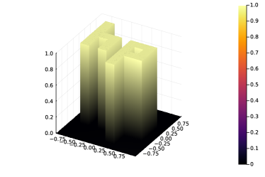
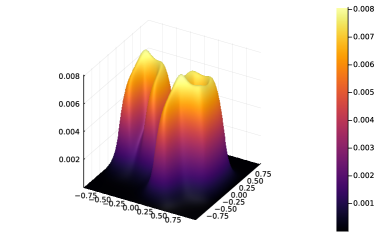
Figure 3: Example PDE with a discontinuous right-hand side $f$ (left) and solution (right) of the screened Poisson equation $-\Delta u+10^{2}u=f$ with a zero Dirichlet boundary condition. By using a $9\times 9$ elements we can resolve the right-hand side exactly, and then use high $p$ to achieve convergence.

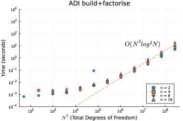
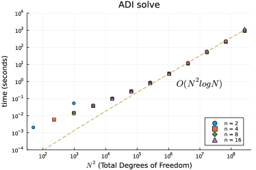
Figure 4: Time taken to build/factorise and solve a discretisation of the Poisson equation in 2D using ADI up to degree $p$, where $n$ is the number of elements. The $x$-axis in the second row of timings is the total number of Degrees of Freedom (DOF) and demonstrates that the complexity is optimal as either $n(=2/h)$ or $p$ become large, and largely only depends on the total number of DOF.

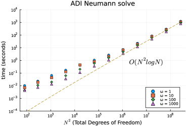
Figure 5: Left: Solution of $-\Delta u+10^{2}u=f$ with a zero Neumann boundary condition, using the same right-hand side as in Figure 3. Right: Solve timings for $n=2$ (two elements) and increasing $p$ with varying choices of $\omega$.

5.2 Complexity analysis

In the previous experiments we observed that Algorithm 2 appears to achieve quasi-optimal complexity. In this section we prove this is guaranteed to be the case. In order to control the complexity, it is necessary to control the number of iterations $J$ which depends on the spectral information of the operators. For simplicity, throughout this section we set $p=q$, i.e we consider an equal discretisation degree in $x$ and $y$. However, we note that all the results generalise.

A key result to derive the complexity of applying the ADI algorithm solely in terms of $N$ and $p$ are bounds on the spectrum for $L^{-\top}M_{Y,p}L^{-1}$ where $L^{\top}L=-\Delta_{Y,p}+(\omega^{2}/2)M_{Y,p}$. This allows us to derive the asymptotic behaviour for $J$.

Lemma 5.3 (Spectrum).

Consider the interval domain $(a,b)$ and a family of quasi-uniform subdivisions $\{\mathcal{T}_{h}\}_{h}$ of the interval, where $h$ denotes the mesh size (the minimum diameter of all the cells in the mesh) [12, Def. 4.4.13]. For the (screened) Poisson equation with Neumann boundary conditions consider the quasimatrix ${\bf Y}_{0:p}(x)={\bf C}_{0:p}(x)$ and with a zero Dirichlet boundary condition consider ${\bf Y}_{0:p}(x)={\bf Q}_{0:p}(x)$ where $p$ is the truncation degree on each element. Suppose that $L^{\top}L=A_{Y,p}\coloneqq(-\Delta)_{Y,p}+(\omega^{2}/2)M_{Y,p}$ where $\omega\neq 0$ in the case of Neumann boundary conditions. Then

(22) $$\sigma(L^{-\top}M_{Y,p}L^{-1})\subseteq\left[\frac{2h^{2}}{24p^{4}+\omega^{2}h^{2}},C\right],$$

where $C=\min((b-a)^{2}/\pi^{2},\max(1,2/\omega^{2}))$ in the case of a zero Dirichlet boundary condition and $C=\max(1,2/\omega^{2})$ in the case of a zero Neumann boundary condition.

Proof 5.4.

The eigenvalue problem to consider is

(23) $$L^{-\top}M_{Y,p}L^{-1}{\bf v}_{p}=\lambda{\bf v}_{p},$$

where $\lambda$ and ${\bf v}_{p}$ denote an eigenvalue and corresponding eigenvector, respectively. First note that $L^{-\top}M_{Y,p}L^{-1}$ is congruent to a symmetric positive-definite matrix and, therefore, $\lambda$ must be real and positive. Left multiplying Eq. 23 by $L^{\top}$, and considering ${\bf w}_{p}=L^{-1}{\bf v}_{p}$, we deduce that

(24) $$M_{Y,p}{\bf w}_{p}=-\lambda\Delta_{Y,p}{\bf w}_{p}+\frac{\lambda\omega^{2}}{2}M_{Y,p}{\bf w}_{p}.$$

For $w\in H^{1}(a,b)$, let $|w|_{H^{1}(a,b)}\coloneqq\|w^{\prime}\|_{L^{2}(a,b)}$. Left multiplying Eq. 24 by ${\bf w}^{\top}_{p}$ implies that

(25) $$\|{\bf Y}_{0:p}{\bf w}_{p}\|^{2}_{L^{2}(a,b)}=\lambda|{\bf Y}_{0:p}{\bf w}_{p}|^{2}_{H^{1}(a,b)}+\frac{\lambda\omega^{2}}{2}\|{\bf Y}_{0:p}{\bf w}_{p}\|^{2}_{L^{2}(a,b)}.$$

(Upper bound). The upper bound can be split into three cases: (I) a zero Dirichlet boundary condition, (II) $0<\omega^{2}<2$, and (III) $\omega^{2}\geq 2$. In case (I) then ${\bf Y}_{0:p}(a){\bf w}_{p}={\bf Y}_{0:p}(b){\bf w}_{p}={\bf Q}_{0:p}(a){\bf w}_{p}={\bf Q}_{0:p}(b){\bf w}_{p}=0$. Hence the Poincaré inequality (with the optimal Poincaré constant) implies that [36]

(26) $$\frac{\pi^{2}}{(b-a)^{2}}\|{\bf Y}_{0:p}{\bf w}_{p}\|^{2}_{L^{2}(a,b)}\leq|{\bf Y}_{0:p}{\bf w}_{p}|^{2}_{H^{1}(a,b)}\leq\lambda^{-1}\|{\bf Y}_{0:p}{\bf w}_{p}\|^{2}_{L^{2}(a,b)}.$$

Thus $\lambda\leq(b-a)^{2}/\pi^{2}$. In cases (II) and (III) we see that

(27) $$\begin{split}C^{-1}\|{\bf Y}_{0:p}{\bf w}_{p}\|^{2}_{L^{2}(a,b)}&\leq|{\bf Y}_{0:p}{\bf w}_{p}|^{2}_{H^{1}(a,b)}+\frac{\omega^{2}}{2}\|{\bf Y}_{0:p}{\bf w}_{p}\|^{2}_{L^{2}(a,b)}\\ &=\lambda^{-1}\|{\bf Y}_{0:p}{\bf w}_{p}\|^{2}_{L^{2}(a,b)},\end{split}$$

where $C^{-1}=\omega^{2}/2$ in case (II) and $C^{-1}=1$ in case (III). Thus $\lambda\leq\max(1,2/\omega^{2})$. Combining the results from cases (I)–(III), we conclude the upper bound on the spectrum.

(Lower bound). Consider a degree $p$ polynomial $\pi_{p}$ defined on the interval $(0,h)$. Then the following inverse inequality holds [37, Th. 3.91]:

(28) $$|\pi_{p}|_{H^{1}(0,h)}\leq 2\sqrt{3}h^{-1}p^{2}\|\pi_{p}\|_{L^{2}(0,h)}.$$

Consequently, Eq. 28 implies that

(29) $$\begin{split}\lambda^{-1}\|{\bf Y}_{0:p}{\bf w}_{p}\|^{2}_{L^{2}(a,b)}&=|{\bf Y}_{0:p}{\bf w}_{p}|^{2}_{H^{1}(a,b)}+\frac{\omega^{2}}{2}\|{\bf Y}_{0:p}{\bf w}_{p}\|^{2}_{L^{2}(a,b)}\\ &\leq 12h^{-2}p^{4}\|{\bf Y}_{0:p}{\bf w}_{p}\|^{2}_{L^{2}(a,b)}+\frac{\omega^{2}}{2}\|{\bf Y}_{0:p}{\bf w}_{p}\|^{2}_{L^{2}(a,b)}.\end{split}$$

Hence $\lambda\geq\frac{2h^{2}}{24p^{4}+\omega^{2}h^{2}}$.

From the formula of $J$ we arrive at the following:

Lemma 5.5.

Under the conditions of the previous proposition, $O(J)=O(\log N\log\epsilon^{-1})$.

This allows us to establish complexity results:

Theorem 5.6.

Precomputation in Algorithm 2 can be accomplished in $O(nN^{2}+JN)$ operations, where we assume we can compute special functions (hyperbolic trigonometric functions, ${\rm log}$, and the elliptic integral ${\rm dn}$) in $O(1)$ operations, where $N$ is the maximal degrees of freedom of either coordinate direction. Solve in Algorithm 2 can be accomplished in $O(JN^{2})$ operations. Using the bound on $J$ in the previous result shows quasi-optimal complexity for the precomputation as $p\rightarrow\infty$.

Proof 5.7.

(Precomputation): The $B^{3}$-Arrowhead matrices involved can be viewed as square banded matrices with bandwidth $O(n)$ and dimensions that scale like $O(N)$, hence line (1) can be computed in $O(nN^{2})$ operations following [15]. By the complexity of compute reverse Cholesky factorisations of $B^{3}$-Arrowhead matrices we know lines (4–6) take $O(JN)$ operations.

(Solve): Multiplying and inverting $B^{3}$-Arrowhead matrices can be done on each column of $W_{j}$ in $O(N)$ operations which immediately gives the result.

Remark 5.8.

Using inverse iteration it is likely that the precomputation cost can be reduced to $O(N)$ operations but this would require more information on the gap between the eigenvalues. Note also that eigenvalue algorithms have errors which can alter the number of iterations $J$ but we have neglected taking this into consideration as it is unlikely to have a material impact.

6 Transforms and time-evolution

To utilise ADI solvers in an iterative framework for nonlinear elliptic PDEs or in time-evolution problem it is essential to be able to efficiently transform between values on a grid and coefficients. To accomplish this we need the following transforms in 1D and 2D:

1. Given a grid, find the expansion coefficients of the right-hand side into piecewise Legendre polynomials.

2. Given coefficients of the solution in the basis ${\bf Q}$, find the values on a grid.

The first stage can be tackled by transforming from values at piecewise Chebyshev grids to Chebyshev coefficients using the DCT, and thence to Legendre coefficients via a fast Chebyshev–Legendre transform [2, 26, 41]. Denote the $p$ Chebyshev points of the first kind as

$${\bf x}_{p}^{\rm T}\coloneqq\left[{\sin\!\left({\pi{p-2k+1\over 2p}}\right)}\right]_{k=1}^{p}.$$

We denote the transform from Chebyshev points to Legendre coefficients (which combines the DCT with the Chebyshev–Legendre transform) as ${\cal F}_{p}$ and its inverse as ${\cal F}_{p}^{-1}$. That is: if $f(x)={\bf P}_{0:p}{\bf c}$ then ${\bf c}={\cal F}_{p}f({\bf x}_{p}^{\rm T}).$ Now for multiple elements we affine transform the grid to get a matrix of values. That is, for a matrix of grid points $X_{p}^{n}=[{\bf x}_{p}^{1}|\cdots|{\bf x}_{p}^{n}]$ we transform each column: ${\cal F}_{p}f(X_{p}^{n})$. Reinterpreting this matrix as a block-vector, whose rows correspond to blocks, gives the coefficients in the basis ${\bf P}^{\bf x}$. That is, we use

$${\rm vec}(({\cal F}_{p}f(X_{p}^{n}))^{\top})$$

where ${\rm vec}:{\mathbb{R}}^{p\times n}\rightarrow{\mathbb{R}}^{pn}$ is the operator from matrices to block vectors that concatenates the columns.

To extend this to two dimensions, we use the grids ${\bf x}={\rm vec}^{-1}(X_{p}^{n})$ and ${\bf y}={\rm vec}^{-1}(X_{q}^{m})$ and hence we want to transform from a matrix of values on the tensor product grid i.e.,

$$F\coloneqq\left[{f(x_{k},y_{j})}\right]_{k=1,j=1}^{k=pn,j=qm}.$$

The 2D transform is then ${\cal F}_{p}^{n}F({\cal F}_{q}^{m})^{\top}.$

The second stage can be accomplished by first computing the coefficients in a piecewise Legendre basis via applying the matrix $R^{\bf x}$, transforming to Chebyshev coefficients via a fast Legendre–Chebyshev transform, then applying the inverse DCT to recover the values on a Chebyshev grid. That is, if we have

$$u(x,y)={\bf Q}_{0:p}(x)U{\bf Q}_{0:q}(y)^{\top}$$

then we can transform back to a grid via

$$u({\bf x},{\bf y}^{\top})=({\cal F}_{p}^{n})^{-1}R^{\bf x}U(R^{\bf y})^{\top}{\cal F}_{q}^{-\top}.$$

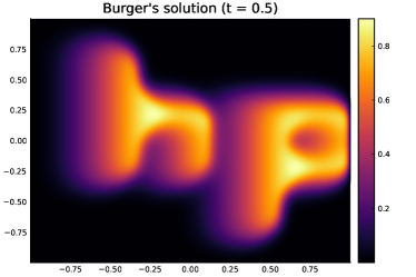
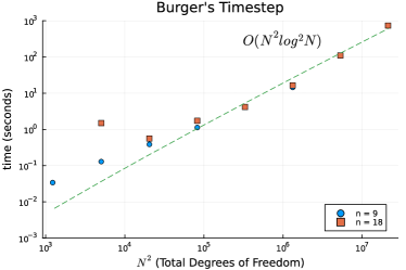
Figure 6: Left: Solution of Burgers equation $u_{t}+uu_{x}=\epsilon\Delta u$ with a zero Dirichlet boundary condition, where the initial condition is the discontinuous right-hand side as in Figure 3, with $\epsilon=0.1$. Right: time taken for a single time-step, using a splitting method where the linear part is solved using implicit Euler and the nonlinear part with explicit Euler, after transforming back to a grid.

As an example of the utility of fast transforms, Figure 6 considers the classic Burgers’ equation:

$$(u_{t}+uu_{x})(x,y,t)=\epsilon\Delta u(x,y,t)$$

with a zero Dirichlet boundary condition and a discontinuous initial condition. We discretise in time using a simple splitting method, taking a linear step via implicit Euler followed by a nonlinear step via explicit Euler:

$$u_{k+1/2}(x,y) =(I-(\delta t)\epsilon\Delta)^{-1}u_{k}(x,y),$$

$$u_{k+1}(x,y) =(u_{k+1/2}+(\delta t)u_{k+1/2,x}u_{k+1/2})(x,y).$$

We represent $u_{k}(x,y)$ as a matrix $U_{k}$ containing coefficients in an expansion of tensor products of piecewise Legendre polynomials, i.e., using the basis ${\bf P}^{\bf x}$. The half time-steps $u_{k+1/2}(x,y)$ are then represented as a matrix $U_{k+1/2}$ giving coefficients in tensor products of ${\bf Q}^{\bf x}$, where the coefficients are computed using ADI as described above. To determine $u_{k+1/2}(x,y)$ on a grid we simply convert down to Legendre and then apply the inverse fast Legendre transform, that is that values are approximated by:

$$V_{k+1/2}\coloneqq{\cal F}^{-1}RU_{k+1/2}R^{\top}{\cal F}^{-\top}.$$

For $u_{(k+1/2),x}(x,y)$ we compute its Legendre coefficients using the derivative matrix alongside the conversion matrix, that is:

$$V_{k+1/2,x}\coloneqq{\cal F}^{-1}DU_{k+1/2}R^{\top}{\cal F}^{-\top}.$$

We can then determine the Legendre coefficients $U_{k+1}$ as

$$U_{k+1}\coloneqq{\cal F}\left[{V_{k+1/2}+(\delta t)V_{k+1/2,x}\otimes V_{k+1/2}}\right].$$

The right-hand side plot in Fig. 6 roughly demonstrates the predicted $O(N^{2}\log^{2}N)$ complexity.

7 Future work

We have constructed the first provably quasi-optimal complexity $hp$-FEM method for the (screened) Poisson equation on a rectangle, built on taking advantage of the sparsity structure. There are some clear extensions to this work:

1. In one dimension we can easily incorporate variable coefficients for Schrödinger equations of the form:

   $$\left\langle{v^{\prime},u^{\prime}}\right\rangle+\left\langle{v,a(x)u}\right\rangle=\left\langle{v,f}\right\rangle,$$

   by expanding $a$ with a piecewise polynomial, that is, a polynomial within each element. The discretisation will still lead to $B^{3}$-Arrowhead matrices but with bandwidths proportional to the polynomial degree. An effective scheme would be to subdivide the elements in such a way that the polynomial degree (and hence the bandwidths) of the approximation is bounded. However, this is of limited utility to higher dimensions without incorporating iterative methods/preconditioners as only rank-2 PDEs (in the sense of [40]) lead to Sylvester’s equations and we do not necessarily have control on the spectrum needed by ADI.

2. For non-positive definite but symmetric operators, it is possible to do $L^{\top}DL$ factorisations of the $B^{3}$-Arrowhead matrices in optimal complexity. However, this may lead to ill-conditioning. Unfortunately, stable factorisations such as $QL$ only achieve $O(pn+n^{3})$ complexity as there is fill-in in the top blocks.

3. Fortunato and Townsend [18] also considered Poisson equations posed on cylinders and cubes. What we have discussed can be combined with their techniques to tackle these 3D problems.

Appendix A Recurrences

In this appendix we provide the formulae for the entries in the matrices Eq. 3, Eq. 4–Eq. 5 and Eq. 6–Eq. 7. From [16, 18.9.8], we have that

(30) $$W_{k}(x)={1\over 2k+3}(P_{k}(x)-P_{k+2}(x)).$$

Thus we deduce that the entries in Eq. 3 are

$$\underbrace{[W_{0},W_{1},W_{2},\ldots]}_{\bf W}=\underbrace{[P_{0},P_{1},P_{2},\ldots]}_{\bf P}\underbrace{\begin{bmatrix}1/3\\ 0&1/5\\ -1/3&0&1/7\\ &-1/5&0&1/9\\ &&\ddots&\ddots&\ddots\end{bmatrix}}_{L_{W}}.$$

Next we derive the entries in Eq. 4–Eq. 5. Consider the reference cell $(-1,1)$. Then there exists two hat functions with nonzero support, $h_{0}(x)=(1-x)/2$ and $h_{1}(x)=(x+1)/2$. Since these are degree one polynomials then, for $k\geq 2$, $\langle P_{k},h_{j}\rangle=0$, and hence $R_{k0}={\bf 0}$. Moreover, we have that $M_{00}=2$, $M_{11}=2/3$, $\langle P_{0},h_{j}\rangle=1$, and $\langle P_{1},h_{j}\rangle=(-1)^{j+1}/3$ for $j\in\{0,1\}$. A scaling argument reveals that these entries are independent of the size of the element. Hence $R_{k0}\in\mathbb{R}^{n\times(n+1)}$ and the entries in Eq. 4 are

(31) $$R_{00}=\begin{bmatrix}1/2&1/2&&\\ &\ddots&\ddots&\\ &&1/2&1/2\end{bmatrix},\;\;R_{10}=\begin{bmatrix}-1/2&1/2&&\\ &\ddots&\ddots&\\ &&-1/2&1/2\end{bmatrix},$$

Moreover, for $j>0$, $R_{kj}\in\mathbb{R}^{n\times n}$ and from Eq. 30 we deduce the entries in Eq. 5 are

(32) $$-R_{(k+2)j}=R_{kj}=\begin{bmatrix}\frac{1}{1+2j}&&\\ &\ddots&\\ &&\frac{1}{1+2j}\end{bmatrix}\;\;\text{if}\;\;k=j\pm 1,$$

and otherwise $R_{kj}={\bf 0}$.

To compute the entries in Eq. 6–Eq. 7, consider the reference cell $(-1,1)$ and note that $h_{0}^{\prime}(x)=-1/2$, $h_{1}^{\prime}(x)=1/2$ and $W_{k}^{\prime}(x)=-P_{k+1}(x)$, cf. Eq. 2. Let $\delta_{i}=x_{i}-x_{i-1}$ for $i\in\{1:n\}$. Then, by a scaling argument, we deduce that

(33) $$\hskip 14.22636ptD_{00}=\begin{bmatrix}-1/\delta_{1}&1/\delta_{1}&&&\\ &-1/\delta_{2}&1/\delta_{2}&&\\ &&\ddots&\ddots&\\ &&&-1/\delta_{n}&1/\delta_{n}\end{bmatrix}\in\mathbb{R}^{n\times(n+1)}$$

and, for $k>0$,

(34) $$D_{kk}=\begin{bmatrix}-2/\delta_{1}&&&\\ &-2/\delta_{2}&&\\ &&\ddots&\\ &&&-2/\delta_{n}\end{bmatrix}\in\mathbb{R}^{n\times n}\;\;\text{with $D_{kj}={\bf 0}$ if $k\neq j$}.$$

References

- [1] R. A. Adams and J. J. Fournier, Sobolev spaces, Elsevier, 2003.
- [2] B. K. Alpert and V. Rokhlin, A fast algorithm for the evaluation of Legendre expansions, SIAM Journal on Scientific and Statistical Computing, 12 (1991), pp. 158–179.
- [3] A. Averbuch, M. Israeli, and L. Vozovoi, A fast Poisson solver of arbitrary order accuracy in rectangular regions, SIAM Journal on Scientific Computing, 19 (1998), pp. 933–952, https://doi.org/10.1137/S1064827595288589.
- [4] I. Babuška, A. Craig, J. Mandel, and J. Pitkäranta, Efficient preconditioning for the -version finite element method in two dimensions, SIAM Journal on Numerical Analysis, 28 (1991), pp. 624–661.
- [5] I. Babuška and M. Suri, The and - versions of the finite element method, basic principles and properties, SIAM Review, 36 (1994), pp. 578–632, https://doi.org/10.1137/1036141.
- [6] I. Babuška and B. A. Szabó, Lecture notes on finite element analysis, 1983–1985.
- [7] S. Beuchler, C. Pechstein, and D. Wachsmuth, Boundary concentrated finite elements for optimal boundary control problems of elliptic PDEs, Computational Optimization and Applications, 51 (2012), pp. 883–908, https://doi.org/10.1007/s10589-010-9370-2.
- [8] S. Beuchler and V. Pillwein, Sparse shape functions for tetrahedral -FEM using integrated Jacobi polynomials, Computing, 80 (2007), pp. 345–375, https://doi.org/10.1007/s00607-007-0236-0.
- [9] S. Beuchler, V. Pillwein, J. Schöberl, and S. Zaglmayr, Sparsity optimized high order finite element functions on simplices, Springer, 2012, https://doi.org/10.1007/978-3-7091-0794-2_2.
- [10] S. Beuchler and J. Schoeberl, New shape functions for triangular -FEM using integrated Jacobi polynomials, Numerische Mathematik, 103 (2006), pp. 339–366, https://doi.org/10.1007/s00211-006-0681-2.
- [11] E. Braverman, M. Israeli, A. Averbuch, and L. Vozovoi, A fast 3D Poisson solver of arbitrary order accuracy, Journal of Computational Physics, 144 (1998), pp. 109–136, https://doi.org/10.1006/jcph.1998.6001.
- [12] S. C. Brenner and L. R. Scott, The Mathematical Theory of Finite Element Methods, vol. 15 of Texts in Applied Mathematics, Springer New York, New York, NY, 3 ed., 2008, https://doi.org/10.1007/978-0-387-75934-0.
- [13] P. D. Brubeck and P. E. Farrell, A scalable and robust vertex-star relaxation for high-order FEM, SIAM Journal on Scientific Computing, 44 (2022), pp. A2991–A3017, https://doi.org/10.1137/21M1444187.
- [14] B. L. Buzbee, G. H. Golub, and C. W. Nielson, On direct methods for solving Poisson’s equations, SIAM Journal on Numerical analysis, 7 (1970), pp. 627–656, https://doi.org/10.1137/0707049.
- [15] C. Crawford, Reduction of a band-symmetric generalized eigenvalue problem, Communications of the ACM, 16 (1973), pp. 41–44.
- [16] NIST Digital Library of Mathematical Functions. https://dlmf.nist.gov/, Release 1.1.11 of 2023-09-15, https://dlmf.nist.gov/. F. W. J. Olver, A. B. Olde Daalhuis, D. W. Lozier, B. I. Schneider, R. F. Boisvert, C. W. Clark, B. R. Miller, B. V. Saunders, H. S. Cohl, and M. A. McClain, eds.
- [17] M. Dubiner, Spectral methods on triangles and other domains, Journal of Scientific Computing, 6 (1991), pp. 345–390, https://doi.org/10.1007/BF01060030.
- [18] D. Fortunato and A. Townsend, Fast Poisson solvers for spectral methods, IMA Journal of Numerical Analysis, 40 (2020), pp. 1994–2018.
- [19] E. Gagliardo, Caratterizzazioni delle tracce sulla frontiera relative ad alcune classi di funzioni in variabili, Rendiconti del seminario matematico della universita di Padova, 27 (1957), pp. 284–305.
- [20] A. Gholami, D. Malhotra, H. Sundar, and G. Biros, FFT, FMM, or multigrid? A comparative study of state-of-the-art Poisson solvers for uniform and nonuniform grids in the unit cube, SIAM Journal on Scientific Computing, 38 (2016), pp. C280–C306, https://doi.org/10.1137/15M1010798.
- [21] A. Gillman, P. M. Young, and P.-G. Martinsson, A direct solver with complexity for integral equations on one-dimensional domains, Frontiers of Mathematics in China, 7 (2012), pp. 217–247, https://doi.org/10.1007/s11464-012-0188-3.
- [22] P. Houston, C. Schwab, and E. Süli, Discontinuous hp-finite element methods for advection-diffusion-reaction problems, SIAM Journal on Numerical Analysis, 39 (2002), pp. 2133–2163, https://doi.org/10.1137/S0036142900374111.
- [23] I. Huismann, J. Stiller, and J. Fröhlich, Scaling to the stars–a linearly scaling elliptic solver for -multigrid, Journal of Computational Physics, 398 (2019), p. 108868, https://doi.org/10.1016/j.jcp.2019.108868.
- [24] L. Jia, H. Li, and Z. Zhang, Sparse spectral-Galerkin method on an arbitrary tetrahedron using generalized koornwinder polynomials, Journal of Scientific Computing, 91 (2022), p. 22, https://doi.org/10.1007/s10915-022-01778-y.
- [25] G. E. Karniadakis, G. Karniadakis, and S. Sherwin, Spectral/ element methods for computational fluid dynamics, Oxford University Press on Demand, 2005, https://doi.org/10.1093/acprof:oso/9780198528692.001.0001.
- [26] J. Keiner, Fast Polynomial Transforms, Logos Verlag Berlin GmbH, 2011.
- [27] K. Knook, S. Olver, and I. P. A. Papadopoulos, ADIPoisson.jl, 2024, https://github.com/ioannisPApapadopoulos/ADIPoisson.jl.
- [28] K. Knook, S. Olver, and I. P. A. Papadopoulos, ioannisPApapadopoulos/ADIPoisson.jl: v0.0.2, Feb. 2024, https://doi.org/10.5281/zenodo.10673881.
- [29] J. W. Lottes and P. F. Fischer, Hybrid multigrid/Schwarz algorithms for the spectral element method, Journal of Scientific Computing, 24 (2005), pp. 45–78, https://doi.org/10.1007/s10915-004-4787-3.
- [30] R. E. Lynch, J. R. Rice, and D. H. Thomas, Direct solution of partial difference equations by tensor product methods, Numerische Mathematik, 6 (1964), pp. 185–199, https://doi.org/10.1007/BF01386067.
- [31] P.-G. Martinsson, A fast direct solver for a class of elliptic partial differential equations, Journal of Scientific Computing, 38 (2009), pp. 316–330, https://doi.org/10.1007/s10915-008-9240-6.
- [32] P.-G. Martinsson, Fast direct solvers for elliptic PDEs, SIAM, 2019, https://doi.org/10.1137/1.9781611976045.
- [33] A. McKenney, L. Greengard, and A. Mayo, A fast Poisson solver for complex geometries, Journal of Computational Physics, 118 (1995), pp. 348–355, https://doi.org/10.1006/jcph.1995.1104.
- [34] S. A. Orszag, Spectral methods for problems in complex geometrics, in Numerical methods for partial differential equations, Elsevier, 1979, pp. 273–305.
- [35] L. F. Pavarino, Additive Schwarz methods for the -version finite element method, Numerische Mathematik, 66 (1993), pp. 493–515, https://doi.org/10.1007/BF01385709.
- [36] L. E. Payne and H. F. Weinberger, An optimal Poincaré inequality for convex domains, Archive for Rational Mechanics and Analysis, 5 (1960), pp. 286–292, https://doi.org/10.1007/BF00252910.
- [37] C. Schwab, -and -finite element methods: Theory and applications in solid and fluid mechanics, Clarendon Press, 1998.
- [38] B. Snowball and S. Olver, Sparse spectral and finite element methods for partial differential equations on disk slices and trapeziums, Studies in Applied Mathematics, 145 (2020), pp. 3–35, https://doi.org/10.1111/sapm.12303.
- [39] B. Szabó and I. Babuška, Introduction to finite element analysis: formulation, verification and validation, vol. 35, John Wiley & Sons, 2011.
- [40] A. Townsend and S. Olver, The automatic solution of partial differential equations using a global spectral method, Journal of Computational Physics, 299 (2015), pp. 106–123.
- [41] A. Townsend, M. Webb, and S. Olver, Fast polynomial transforms based on Toeplitz and Hankel matrices, Mathematics of Computation, 87 (2018), pp. 1913–1934.