Electronic structure and magnetism in $P4/nmm$ KCoO₂

Abstract

KCoO₂ has been found in 1975 to exist in a unique structure with $P4/nmm$ spacegroup with Co in a square pyramidal coordination with the Co atoms in the plane linked by O in a square arrangement reminiscent of the cuprates but its electronic structure has not been studied until now. Unlike Co atoms in LiCoO₂ and NaCoO₂ in octahedral coordination, which are non-magnetic band structure insulators, the unusual coordination of $d^{6}$ Co³⁺ in KCoO₂ is here shown to lead to a magnetic stabilization of an insulating structure with high magnetic moments of $4\mu_{B}$ per Co. The electronic band structure is calculated using the quasiparticle self-consistent (QS)$GW$ method and the basic formation of magnetic moments is explained in terms of the orbital decomposition of the bands. The optical dielectric function is calculated using the Bethe-Salpeter equation including only transitions between equal spin bands. The magnetic moments are shown to prefer an antiferromagnetic ordering along the [110] direction. Exchange interactions are calculated from the transverse spin susceptibility and a rigid spin approximation. The Néel temperature is estimated using the mean-field and Tyablikov methods and found to be between $\sim$100 and $\sim$250 K. The band structure in the AFM ordering can be related to the FM ordering by band folding effects. The optical spectra are similar in both structures and show evidence of excitonic features below the quasiparticle gap of $\sim$4 eV.

I Introduction

Among the alkali oxocobaltates, LiCoO₂ and NaCoO₂ have received much more attention than the larger cation ones because of their role in Li-ion batteries and the reported superconductivity in hydrated Na_1/3CoO₂:H₂O_y. Both of these exhibit the layered $R\bar{3}m$ structure, which can be viewed as consisting of edge sharing, octahedrally coordinated CoO₂ layers with a triangular Co-lattice stacked in an ABC stacking with intercalated Li or Na. The octahedral coordination, splitting $d$-levels in a six-fold degenerate $t_{2g}$ and a four-fold degenerate $e_{g}$ level, leads to a simple non-magnetic insulating band structure for the $d^{6}$ configuration of Co³⁺ resulting from Li or Na donating their electron to the CoO₂ planes. However, starting with K, the alkali ions are too large to fit in this structure. Only half the amount of K can be maintained in between CoO₂ layer in this K_xCoO₂ structure. For larger $x$, this structure becomes unstable and other structures were reported. In 1975, two different synthesis methods for KCoO₂ were reported and led to two totally different crystal structures with different Co-coordination. The first is a unique layered structure with square pyramidal coordination, with the $P4/nmm$ space group [1]. The other is a stuffed cristobalite type structure in which Co is tetrahedrally coordinated with O in an open network of corner sharing tetrahedra, filled with K ions. Two related forms with space groups $I\bar{4}$ and $I\bar{4}2d$ were found and called respectively $\beta$ and $\alpha$-KCoO₂ [2]. Besides these two papers, there seems to be no other studies reported on KCoO₂. Only very recently, a new synthesis method was developed for KCoO₂ in the pyramidal coordination and $P4/nmm$ spacegroup [3].

Because of the occurrence of a square coordination of CoO₂, which resembles that of CuO₂ in high-$T_{c}$ materials, this phase may be of interest for non-conventional superconductivity. The occurrence of Co³⁺ with a $d^{6}$ configuration in a pyramidal environment is also expected to show a high-spin, thus may have interesting magnetic properties. Here we present first-principles calculations of this material and its magnetic properties.

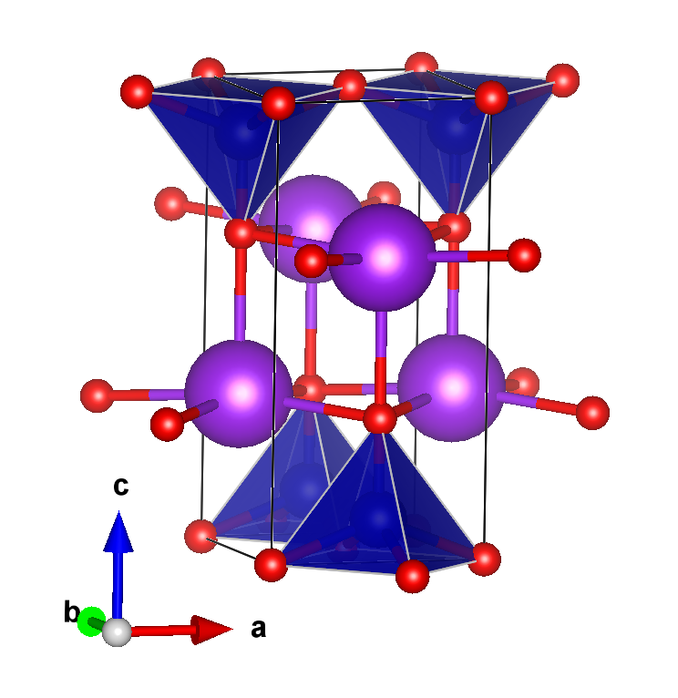
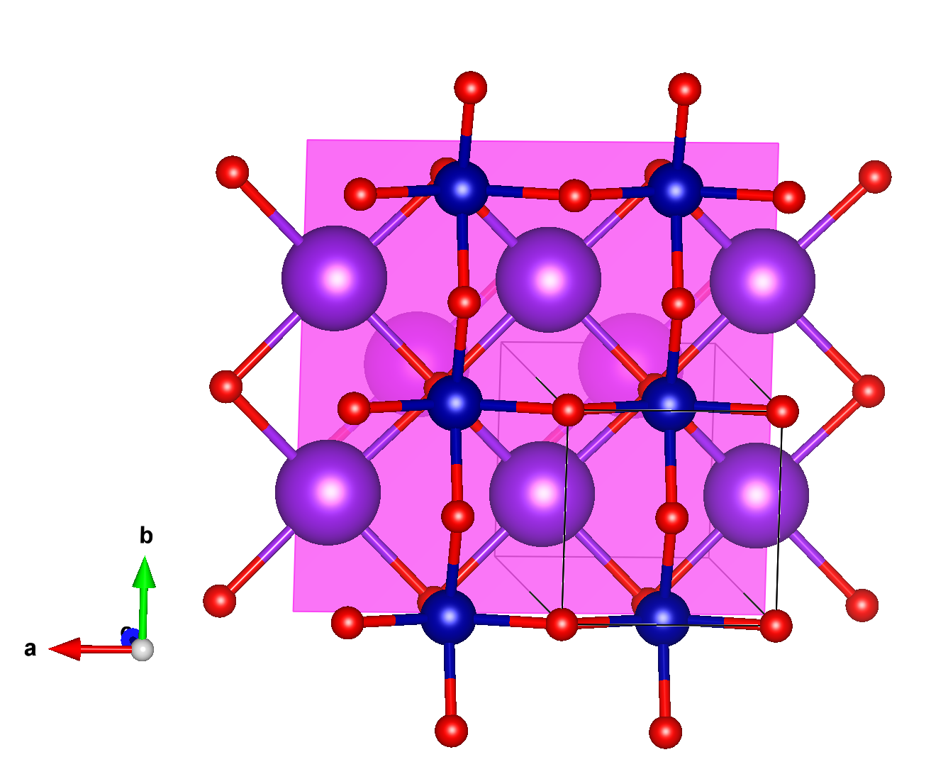
Fig. 1: $P4/nmm$ crystal structure of KCoO₂ in two different projections, the first emphasizing the square pyramidal coordination of Co, and the second projecting on the c-plane emphasizing the Co-O square arrangement reminiscent of the cuprates.

II Computational Methods

The calculations in this study combine density functional theory (DFT) with many-body perturbation theory (MBPT). While DFT is used as a starting point for the electronic structure, the generalized gradient approximation (GGA) (used here in the Perdew-Burke-Ernzerhof (PBE) parametrization [4]) is not sufficiently accurate to make accurate predictions for band gaps and optical properties. To calculate the quasiparticle band structure, we use Hedin’s $GW$ method [5, 6] in which $G$ is the one-electron Green’s function and $W$ is the screened Coulomb interaction. More specifically, we here use the quasiparticle self-consistent version of $GW$ (QS$GW$) [7, 8], which becomes independent of the starting DFT approximation by including a non-local exchange correlation potential extracted from the $GW$ self-energy and updating the non-interacting $H_{0}$ Hamiltonian. By non-interacting, we here mean that the dynamical (energy-dependent) interactions are not included but only a static interaction as in DFT.

The band structure method used to solve the Kohn-Sham equations underlying both the DFT and QS$GW$ method is the full-potential linearized muffin-tin orbital (FP-LMTO) method as implemented in the Questaal codes [9]. This is an augmentation method in which the basis set consists of atom-centered smoothed Hankel function spherical waves [10], augmented inside the muffin-tin spheres with solutions of the radial Schrödinger equation of the all-electron potential at a linearization energy and their energy derivatives. Core states, calculated with atomic boundary conditions at the muffin-tin radius, are thus fully included in the charge density (thereby including core-valence exchange) and semicore states are further included in the basis set as local orbitals with a fixed boundary condition at the sphere radii. Here we include K $3p$ states as local orbitals.

In the LMTO implementation of the $GW$ method, two-point quantities such as the bare and screened Coulomb interaction are expanded in an auxiliary mixed product basis set, which incudes products of partial waves inside the spheres and interstitial plane waves. Such a basis set is more efficient than a plane wave basis set to describe the screening and reduces the need to include high-energy empty bands.

The optical dielectric function is calculated using the Bethe-Salpeter equation (BSE) in the Tamm-Damcoff approximation and using a static $W$ [11] as implemented by Cunningham et al. [12, 13] in the LMTO-basis set within the Questaal package.

The basis set and other convergence parameters are discussed along with the results. A well-converged $\Gamma$-point centered ${\bf k}$-mesh of $8\times 8\times 4$ and the tetrahedron method are used for the Brillouin zone integrations in the DFT calculations. The atom-centered basis set allows us to interpolate the $GW$ self-energy via a Fourier transform to real space and back to any desired k-point even when using a somewhat coarser $5\times 5\times 3$ mesh of points on which the $GW$ self-energy is evaluated. The BSE calculations are performed including 12 valence and 6 conduction bands.

To study the magnetic exchange interactions, we use the approach of Kotani and van Schilfgaarde [14], which extracts the exchange interactions from the transverse spin susceptibility within a rigid spin approximation within each muffin-tin sphere. The non-interacting spin-spin response function is first calculated from the spin-dependent QS$GW$ eigenstates and eigenvalues:

$$\chi_{\bf q}^{0+-}({\bf r},{\bf r}^{\prime},\omega)$$

$$=\sum_{{\bf k}n\downarrow}^{occ}\sum_{{\bf k}^{\prime}n^{\prime}\uparrow}^{unocc}\frac{\Psi^{*}_{{\bf k}n\downarrow}({\bf r})\Psi_{{\bf k}^{\prime}n^{\prime}\uparrow}({\bf r})\Psi_{{\bf k}^{\prime}n^{\prime}\uparrow}^{*}({\bf r}^{\prime})\Psi_{{\bf k}n\downarrow}({\bf r}^{\prime})}{\omega-(\epsilon_{{\bf k}^{\prime}n^{\prime}\uparrow}-\epsilon_{{\bf k}n\downarrow})+i\delta}$$

$$+\sum_{{\bf k}n\downarrow}^{unocc}\sum_{{\bf k}^{\prime}n^{\prime}\uparrow}^{occ}\frac{\Psi^{*}_{{\bf k}n\downarrow}({\bf r})\Psi_{{\bf k}^{\prime}n^{\prime}\uparrow}({\bf r})\Psi_{{\bf k}^{\prime}n^{\prime}\uparrow}^{*}({\bf r}^{\prime})\Psi_{{\bf k}n\downarrow}({\bf r}^{\prime})}{-\omega-(\epsilon_{{\bf k}n\downarrow}-\epsilon_{{\bf k}^{\prime}n^{\prime}\uparrow)}+i\delta},$$

with ${\bf k}^{\prime}={\bf k}+{\bf q}$. It is then coarse-grained by averaging over the spheres, which constitutes the rigid spin approximation,

$$D^{0}({\bf q},\omega)_{aa^{\prime}}=\int_{a}d^{3}r\int_{a^{\prime}}d^{3}r^{\prime}\bar{e}_{a}({\bf r})\chi_{\bf q}^{0+-}({\bf r},{\bf r}^{\prime},\omega))\bar{e}_{a^{\prime}}({\bf r}^{\prime}),$$ (2)

with $e_{a}({\bf r})=M_{a}({\bf r})/M_{a}$, $M_{a}=\int_{a}d^{3}rM_{a}({\bf r})$, $\bar{e}_{a}=e_{a}({\bf r})/\int_{a}d^{3}r|e_{a}({\bf r})|^{2}$. So the $\bar{e}_{a}({\bf r})\propto e_{a}({\bf r})$ is a vector along the local magnetization density $M_{a}({\bf r})=n_{\uparrow}({\bf r})-n_{\downarrow}({\bf r})$, normalized by the total moment per sphere $M_{a}$, which is normalized by $\int_{a}d^{3}r\bar{e_{a}}({\bf r})e_{a}({\bf r})=1$. Following Antropov [15], the exchange interactions defined by

$$J_{\alpha\beta}({\bf r},{\bf r}^{\prime})=-\frac{\delta^{2}E}{\delta M_{\alpha}({\bf r})\delta M_{\beta}({\bf r}^{\prime})}$$ (3)

corresponds to the inverse of the transverse susceptibility $J=\chi^{-1}$ because the changes in magnetization originate from an external magnetic field and $\chi$ is the response function vs. the external magnetic field. This differs from the above non-interacting susceptibility, which defines the response with respect to the total field, including the one generated by the interactions. Assuming now that the similarly sphere-averaged interaction term is q-independent and site-diagonal, $\bar{U}_{aa^{\prime}}({\bf q},\omega)=\bar{U}_{a}(\omega)\delta_{aa^{\prime}}$ Kotani and van Schilfgaarde show that one can find $\bar{U}_{a}(\omega)$ by requiring to fulfill a sum rule and the $\omega\rightarrow\infty$ asymptotic behavior. This then yields directly the inverse of the interacting $D({\bf q},\omega)$ as

$$[D({\bf q},\omega)]^{-1}_{aa^{\prime}} = \frac{\omega}{M_{a}}\delta_{aa^{\prime}}-\bar{J}_{aa^{\prime}}({\bf q},\omega),$$

$$\bar{J}_{aa^{\prime}}({\bf q},\omega) = -[D^{0}({\bf q},\omega)]^{-1}_{aa^{\prime}}$$

$$+ \left(\sum_{b}M_{b}[D^{0}({\bf q}=0,\omega)]^{-1}_{ba}/M_{a}\right)\delta_{aa^{\prime}}.$$

This $\bar{J}_{aa^{\prime}}$ is closely related to the Heisenberg exchange interactions, as discussed further in [14],

$$[D^{\cal H}({\bf q},\omega)]^{-1}_{aa^{\prime}}=\frac{\omega}{M_{a}}\delta_{aa^{\prime}}-J^{\cal H}({\bf q}),$$ (5)

which suggest taking $J^{\cal H}({\bf q})=J({\bf q},\omega=0)_{aa^{\prime}}$, i.e. the static limit. Here $J_{aa^{\prime}}$ differs from $\bar{J}_{aa^{\prime}}$ only by removing the on-site term of $[D^{0}]^{-1}$. Although, we sketched here the more general presentation of [14] of the enhanced susceptibility, in the end, we obtain the exchange interactions from the static version of the inverse of the bare susceptibility, $[D^{0}]^{-1}$. This is also compatible with the Liechtenstein et al. multiple scattering formulation of the linear response theory [16].

The Heisenberg exchange interactions in real space $J_{a,a^{\prime}}^{0{\bf T}}$ can then be obtained by inverting the Bloch sum $J_{aa^{\prime}}({\bf q})=\sum_{\bf T}e^{i{\bf q}\cdot{\bf T}}J_{a,a^{\prime}}^{0{\bf T}}$, i.e. by an integral over the Brillouin zone. Thus, if we calculate the $J_{aa^{\prime}}({\bf q})$ on a $N\times N\times N$ mesh in the Brillouin zone, then a discrete inverse Fourier transform gives us the $J_{a,a}^{0{\bf T}}$ in a $N\times N\times N$ supercell, or the exchange interactions out to a distance $|{\bm{\tau}}_{a^{\prime}}-{\bm{\tau}}_{a}+{\bf T}_{max}|$ where ${\bm{\tau}}_{a}$ is the position in the unit cell of the atom labeled $a$. ${\bf T}_{max}$ is the largest lattice translation vector corresponding to the superlattice.

We can then use various methods to estimate the critical temperature $T_{c}$, such as the mean-field approximation, or the random phase approximation (RPA) developed by Tyablikov et al. [17] and Callen [18] and more recently used by Rusz et al. [19]. In the case (which occurs here) of several magnetic sites per unit cell, the critical temperature in the mean-field approximation is obtained by diagonalizing the matrix of the $J^{0}_{ab}=\sum_{\bf T}J_{ab}^{0{\bf T}}$, where if $a=b$, the on-site term $J_{aa}^{00}$ is excluded from the sum,

$$\sum_{b}[J_{ab}^{0}-j\delta_{ab}]\langle S_{b}\rangle=0.$$ (6)

The mean-field critical temperature is then given by $k_{B}T_{c}=2j_{max}/3$ with $j_{max}$ the highest eigenvalue [20]. The normalized eigenvectors tell us the relation of the average spins on the sites in the cell, i.e. the type of magnetic ordering. The mean-field critical temperature is used as starting point for the RPA iterative procedure. Typically, the latter gives an underestimate while the mean-field method gives an upper limit.

III Results

III.1 Band structure and magnetic moments in ferromagnetic structure

Fig. 2: Spin-polarized band structure in GGA of KCoO₂ in the $P4/nmm$ phase.

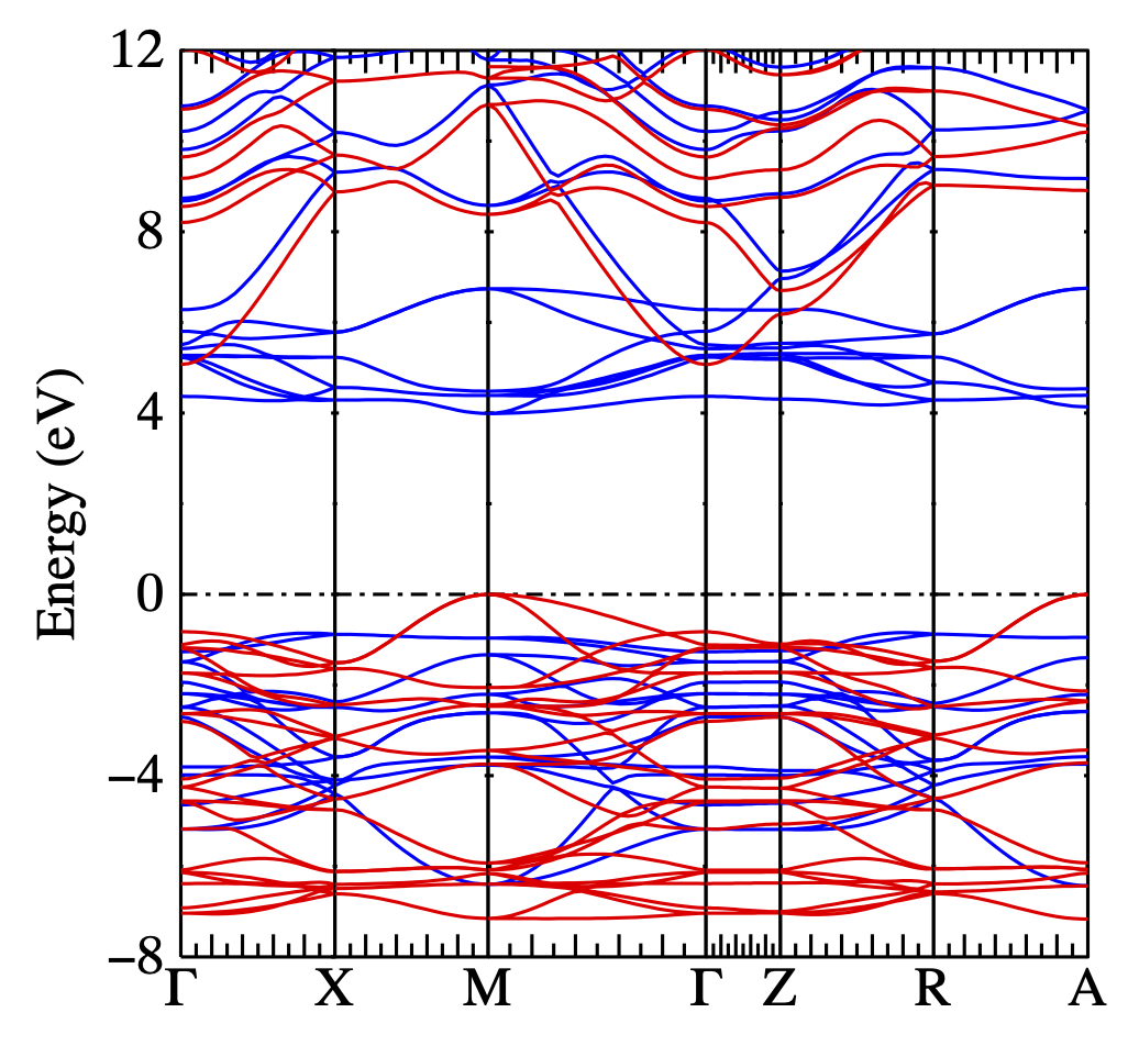
Fig. 3: Band structure of KCoO₂ in QS$GW$ approximation for the $P4/nmm$ structure.

The crystal structure is shown in Fig. 1. There are two types of O, the O₍₁₎ lying close to the K c-plane, which are strongly bonded to the Co in the $z$-direction at a bond distance of 1.741 Å, and the O₍₂₎ which lie in the Co-O₍₂₎ layer and have a bond-length to Co of 2.063 Å. The K-O₁ in-c-plane bond length is 2.732 Å  and along the ${\bf c}$-axis is 2.791 Å. Within spin-polarized GGA, we find a high magnetic moment of 4 $\mu_{B}$ per Co atom and a ferromagnetic semiconductor band structure with a small gap. The high magnetic moment can be understood as follows. Within the square pyramidal coordination of Co and choosing $x$ and $y$ axis pointing toward the oxygen neighbors, the $x^{2}-y^{2}$ orbitals have a large $\sigma$-type antibonding interaction with O-p_x and $p_{y}$ orbitals. In the $D_{4}$ point group they correspond to the $b_{1}$ irreducible representation. The $3z^{2}-r^{2}$ orbital ($a_{1}$) also has a strong interaction with O $p_{z}$ on one side but opposite to it lies a K ion which electrostatically would tend to pull this level down in terms of crystal field splitting. The $xy$ ($b_{2}$) has the weakest interaction, while the $xz,yz$ doubly degenerate $e$ representation has intermediate $\pi$-like interaction. For $d^{6}$ we can thus expect the configuration $b_{2}^{2}e_{\uparrow}^{2}a_{1\uparrow}^{1}b_{1\uparrow}^{1}$ where the spin-polarization of the degenerate $e$ level promotes the exchange splitting of the higher $a_{1}$ and $b_{1}$ level becoming larger than the crystal field splitting.

Table 1: Band gaps in $P4/nmm$ KCoO₂ in QS$GW$ approximation.

type	$k_{v}$	$k_{c}$	spin type	gap (eV)
direct	M	M	$\uparrow\downarrow$	3.99
indirect	M	$\Gamma$	$\uparrow\uparrow$	5.07
direct	M	M	$\uparrow\uparrow$	8.38
direct	$\Gamma$	$\Gamma$	$\uparrow\uparrow$	5.90
indirect	0.8Z-R	M	$\downarrow\downarrow$	4.83
direct	M	M	$\downarrow\downarrow$	4.95
direct	0.8Z-R	0.8Z-R	$\downarrow\downarrow$	5.05

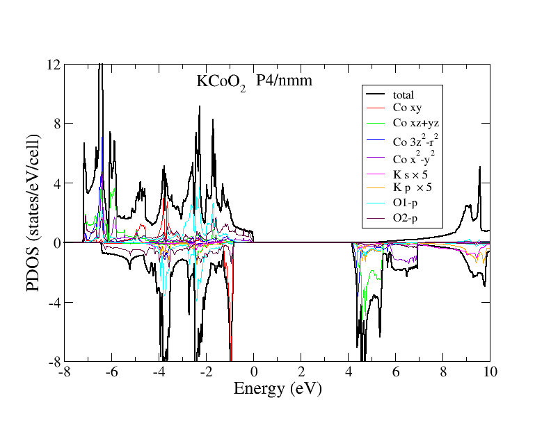
Fig. 4: Total and partial densities of states for KCoO₂ in $P4/nmm$ structure.

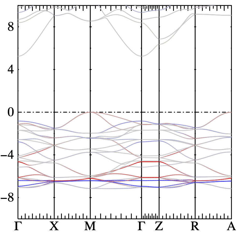
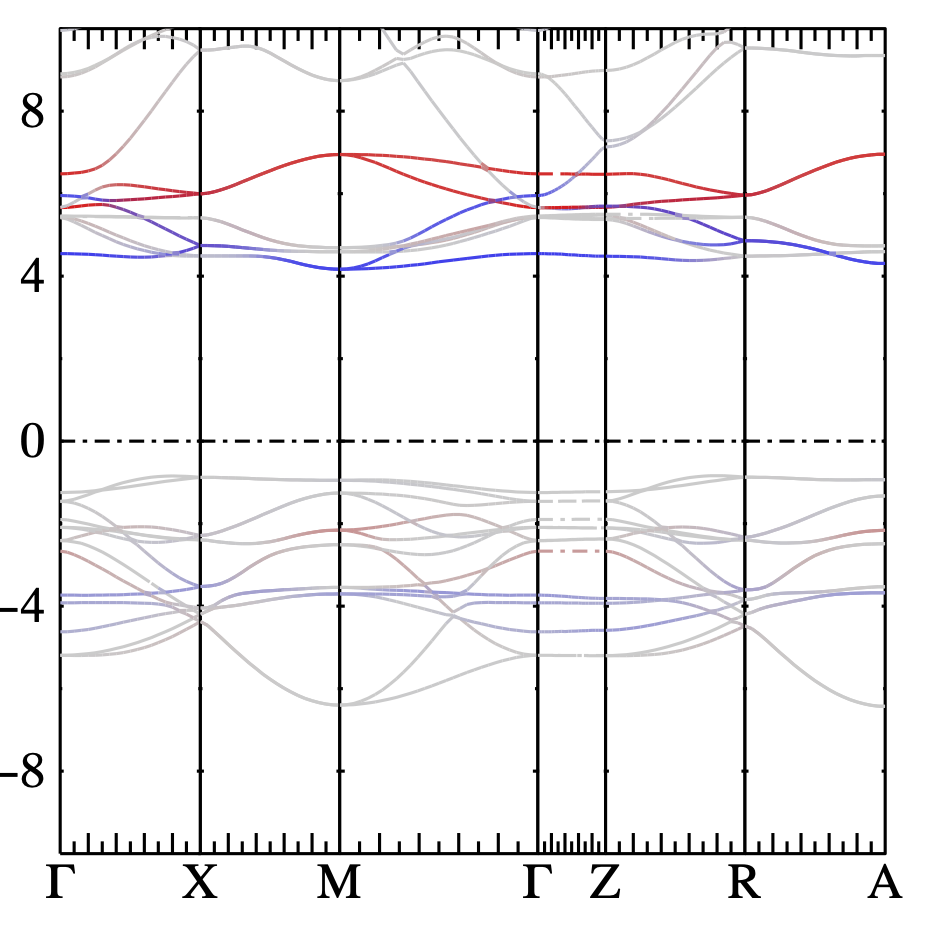
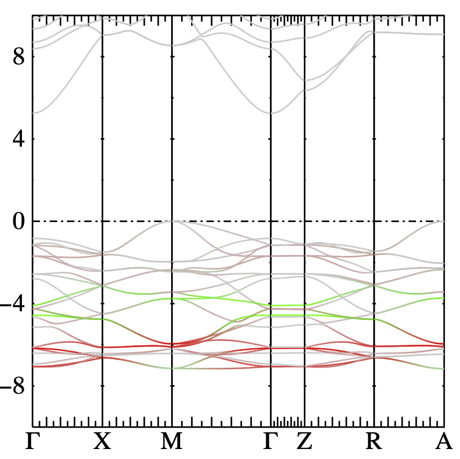
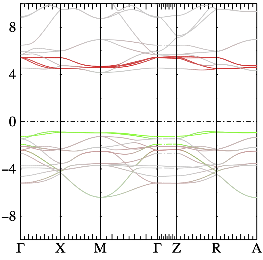
Fig. 5: Orbital weights of Co $d$ of the bands, left for majority and right for minority spin; top row (red) $x^{2}-y^{2}$, (blue) $3z^{2}-r^{2}$, bottom row (red) xz,yz and green (xy).

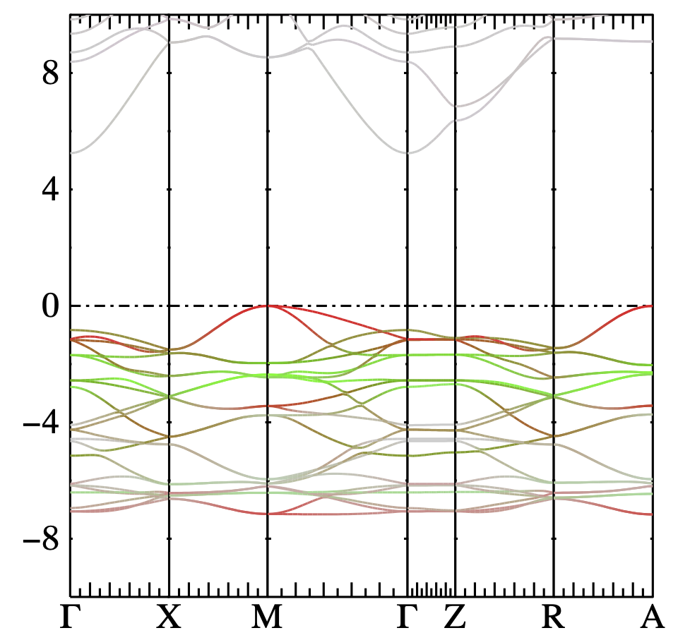
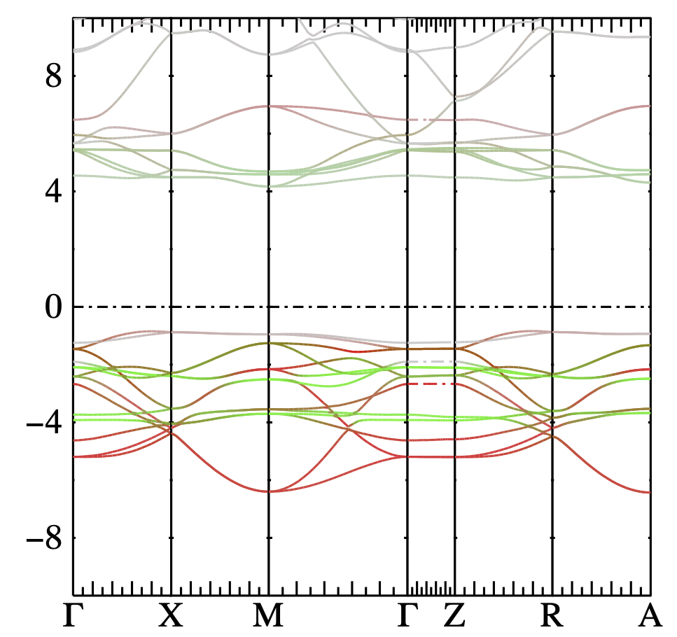
Fig. 6: Orbital weights of O $p$ of the bands for left (majority) and right minority spin; red(O₂), green (O₁)

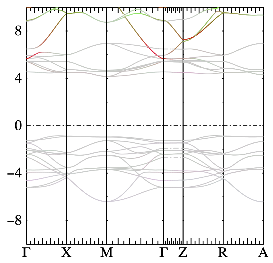
Fig. 7: Orbital weights of K $s$ (red) and $p$ (green) for left (majority) and right (minority) spin.

The spin-polarized band structure at the GGA level is shown in Fig. 2. Interestingly, a small gap opens between spin-up and spin-down bands with rather flat bands. The gap becomes significantly larger in the QS$GW$ method as seen in Fig. 3. We can see that the VBM occurs at $M$ for the majority spin while the CBM has minority spin character. The reason why the VBM occurs at $M$ is that the antibonding interaction of the $x^{2}-y^{2}$ orbitals with O-$p\sigma$ orbitals is optimized at this k-point by the Bloch function phase factors because the same sign lobes point toward the Co for each O along in the square coordination of Co. The majority spin CBM occurs at $\Gamma$. The majority spin highest valence band is quite flat. The majority spin and minority spin band gaps are staggered with respect to each other. The relevant gaps are summarized in Table 1. These calculations used a $2\kappa$ LMTO basis set with smoothed Hankel function envelope functions up to $l=2$ ($spdspd$) for K, and O and ($spdfspd$) for Co. Without the Co-$f$ the gap is slightly higher (4.17 eV).

The total and partial densities of states (PDOS) on various orbitals are shown in Fig. 4. The orbital contributions of the bands are shown in Figs. 5,6 and 7. The PDOS refers to a partial wave decomposition while the bands correspond to a decomposition in muffin-tin-orbital basis functions. These results were obtained with the slightly smaller basis set without the Co-$f$ basis functions but for the qualitative features, this is of no importance. The PDOS and colored band plots provide consistent information.

We can see that the bands with predominantly $xy$ character are filled for both spins. On the other hand, the minority spin $x^{2}-y^{2}$, $3z^{2}-r^{2}$ and $xz,yz$ contributions occur mostly in the empty bands. This is consistent with the above described origin of the large magnetic moment of $4\mu_{B}$. The valence bands also have a significant contribution from O-$p$ as shown in Fig. 6. The K-contributions (shown in Fig. 7), as expected, occur mostly in the conduction band. They do not contribute significantly to the lower lying set of minority spin bands. This is consistent with K donating electron to the CoO₂ layer.

One can see that the majority spin VBM in terms of Co-$d$ has mostly $x^{2}-y^{2}$ contribution but its dominant character is O₍₂₎-$p$. In other words, it is an antibonding state between O${}_{(2)}-p$ in the CoO₂ layer and Co-$d$-$x^{2}-y^{2}$ orbital. The conduction band minimum which nominally occurs at $M$ but corresponds to a rather flat band has predominantly minority spin $3z^{2}-r^{2}$ character on Co and a much smaller O-$p$ character. Thus direct optical transitions from the VBM to the CBM are charge transfer type but would only be allowed for circularly polarized light because they are from spin-up to spin-down. For linearly polarized light the optical transitions would be mostly between the minority spin bands which are both quite flat and have both Co-$d$ character, however with $xy$ character for the VBM of minority spin and $3z^{2}-r^{2}$ character for the conduction band minimum. This would require a change of $m$ orbital character of $\Delta m=2$ and is therefore forbidden in the electric dipole approximation. On the other hand for majority spin, the transitions would be indirect and therefore also forbidden. These optical properties are rather unique and intriguing.

III.2 Optical dielectric function in FM state.

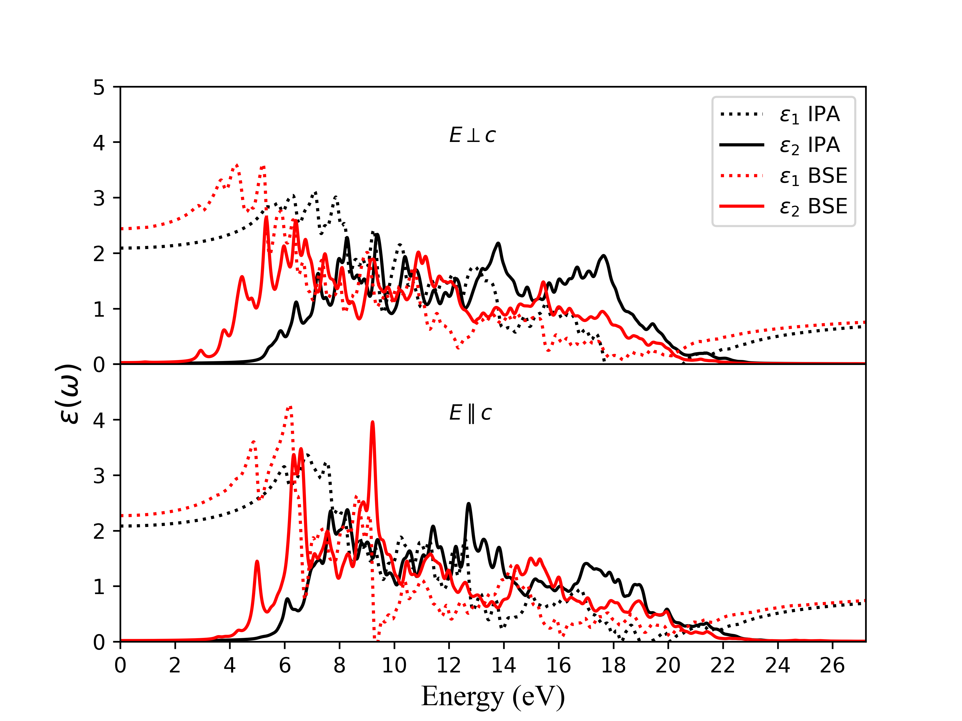
Fig. 8: Optical dielectric function for two polarizations in IPA and BSE, assuming transitions only between the equal spins.

The optical dielectric function was calculated assuming only transitions between majority spin to majority spin states, and minority to minority spins. They were calculated in the independent particle approximation (IPA) and using the Bethe-Salpeter equation (BSE), which includes local field and electron-hole interaction effects. The results are shown for both the real and imaginary part in Fig. 8. Within both IPA and BSE we assume here that the allowed dipole transitions are spin separated. Strictly speaking, the exchange Coulomb interaction matrix elements in the BSE

$$\begin{split}&V_{vc{\bf k}v^{\prime}c^{\prime}{\bf k}^{\prime}}=\\ &\int d(1)d(2)\psi_{v{\bf k}}(1)\psi_{c{\bf k}}(1)^{*}v(|{\bf r}-{\bf r}^{\prime}|)\psi_{v^{\prime}{\bf k}^{\prime}}(2)^{*}\psi_{c^{\prime}{\bf k}^{\prime}}(2)\end{split}$$ (7)

require the valence and conduction band at one k to have the same spin and also at the other k-point because the integral over coordinates (1) or (2) includes spin summation, but the spins of (1) and (2) may differ. So, an interaction between up and down spin is mediated by the exciton exchange interaction. However, if the optical transitions of the separated spins are sufficiently well separated, we may ignore this interaction. This is the approximation we currently are making. Note that for non-spin-polarized systems, this is manifestly not the case since the up-up and down-down transitions are degenerate. However, in that case the spin structure of the excitons is clear [21] and leads to dark spin triplets involving only the $-W$ matrix elements with the screened Coulomb interaction, whereas the spin-singlet ones involve $2\bar{V}-W$ with $\bar{V}$ the microscopic part of the above defined exciton exchange interactions (i.e. excluding the average or long-range macroscopic interaction). At present we include $\bar{V}-W$ but separately for each spin. In the calculation in Fig. 8 we include 24 valence bands and 16 conduction bands. This includes the 12 O-$2p$ bands and 10 Co-$d$ states of each spin.

With this understanding of the approximations made, we now examine the results. First, we may note that the electron-hole effects have a significant impact with excitonic peaks occurring below the quasiparticle gap. Interestingly, there seems to be almost a uniform red shift of $\sim$2 eV from IPA to BSE. Next, we caution that the optical matrix elements of the velocity matrix elements may be overestimated because of difficulties in evaluating the contributions from the non-local self-energy operator of the $GW$ approximation, which require estimating the $d\Sigma/dk$ numerically. This has been found in other systems to overestimate the magnitude of $\varepsilon_{2}(\omega)$ compared to evaluating the $\varepsilon_{2}({\bf q},\omega)$ at finite small ${\bf q}$ and then extrapolating to ${\bf q}\rightarrow 0$ numerically. This then also leads to an overestimate of the $\varepsilon_{1}(\omega)$ below the gap and in particular its limit $\lim_{\omega\rightarrow 0}\varepsilon_{1}(\omega)$, which gives the electronic screening at the static limit. In other words, this “static limit” does not include phonon contributions (conventionally referred to as $\varepsilon_{\infty}$) and corresponds to the square of the index of refraction $n^{2}$ in the range sufficiently well below the gap but higher than any of the phonon modes. Also, at present we cannot yet calculate the transitions between up and down spin bands which would be of great interest in this system but are expected to occur only for circularly polarized light.

III.3 Magnetic ordering

Having established the formation of large magnetic moments as a basic way to stabilize the $d^{6}$ configuration in the unusual pyramidal environment, we now turn to the question of their ordering.

Table 2: Exchange interactions in mRy; $a$ and $b$ label the magnetic atoms in the cell, ${\bf T}$ gives the lattice vector in reduced coordinates, $z$ the number of equivalent neighbors in the star, $J_{ab}^{0{\bf T}}$, he exchange interaction in mRy and the last column gives the cumulative sum, with the last row for a given block of $a,b$ giving the cumulative sum up to $|{\bm{\tau}}_{a}-{\bm{\tau}}_{b}-{\bf T}|<r_{cut}=5$ in units of the in-plane tetragonal lattice constant $a$.

a	b	${\bf T}$	$z$	$J_{ab}^{0{\bf T}}$	$\sum_{\bf T}J_{ab}^{0{\bf T}}$
1	1	$(1,0,0)$	4	$-$0.3725	$-$1.490
1	1	$(1,1,0)$	4	$-$0.0362	$-$1.635
1	1	$(2,0,0)$	4	0.0012	$-1.630$
1	1	…			$-1.561$
1	2	$(0,0,0)$	4	$-$0.0342	$-0.137$
1	2	$(1,0,0)$	8	0.0024	$-0.118$
1	2	$(0,0,1)$	4	$-$0.0024	$-0.127$
1	2	…			$-0.137$

We start from the ferromagnetic unit cell and use the procedure outlined in Sec. II. Table 2 shows some of the near neighbor exchange interactions and their cumulative sums. The $J_{ab}^{0}$ matrix has the form

$$J^{0}=\left(\begin{array}[]{cc}J_{11}^{0}&J_{12}^{0}\\ J_{12}^{0}&J_{11}^{0}\end{array}\right)$$ (8)

with eigenvalues $J_{11}^{0}\pm J_{12}^{0}$, hence we find a mean-field $T_{c}=(2/3k_{B})(J_{11}^{0}-J_{12}^{0})$ of $-149$ K. The negative value indicates that the system actually wants to order antiferromagnetically. Indeed, we find that the average spins on site 1 and 2 are opposite for the eigenvalue $J_{11}^{0}-J_{12}^{0}$. However, we also see that the atoms in (100) neighboring cells also have a negative exchange interaction, which is in fact an order of magnitude larger. Thus, the system would prefer AFM ordering along the [110] direction, with parallel spins in (110) planes and alternating up and down spin from plane to plane but also have the two atoms inside the cell with opposite spin.

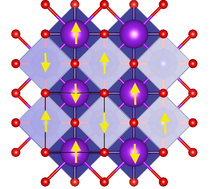
Fig. 9: Spin arrangement on the Co sites, the dark blue squares indicate the Co pyramid of Co slightly below the plane and the light blue ones the Co slightly above the plane. The purple spheres are the K on top of the Co. The red spheres are the O and the yellow arrows indicate the spins on Co.

The spin-arrangement is illustrated in Fig. 9. Within the RPA method, we obtain a slightly lower critical temperature of $131$ K. Given that the dominant exchange interaction corresponds to two Co atoms in line with an O in between, we can interpret this as an antiferromagnetic super-exchange interaction, which might be dominated by the Co-$d$ $x^{2}-y^{2}$ $\sigma$-bonds with O-$p$ orbitals along the line. We can also see that the exchange interactions rapidly decrease beyond the first few neighbors.

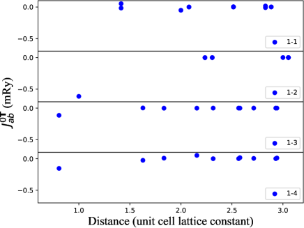
Fig. 10: Exchange interactions in AFM case as function of distance.

Based on the above prediction of antiferromagnetic ordering, we then construct a doubled cell rotated by 45^∘ and recalculate the exchange interactions based on this AFM reference state. We calculated the total energies in the GGA while adding the energy independent self-energy matrix to the one-particle Hamiltonian to have the correct gaps. This gives $E_{AFM}-E_{FM}=-0.240$ eV/Co atom. So, the AFM ordering is definitely preferable. Setting $E_{AFM}-E_{FM}=2zJ_{eff}$ with $z=4$ the number of neighbors, this corresponds to an effective AFM exchange interaction $J_{eff}=-30$ meV. In the mean-field approximation $T_{N}=2J_{eff}/3k_{B}$ and we find $T_{N}\approx 232$ K. However, this assumes there is only an effective nearest neighbor interaction.

Next, we calculate again the exchange interactions from the magnetic susceptibility for this case. We now have four magnetic sites per cell. The exchange interactions between near neighbors are given in Table 3 and plotted as function of distance in Fig. 10.

Table 3: Exchange interactions in [110] AFM cell; magnetic atom labels $a,b$, lattice vector (in Cartesian coordinates and units of $a$ in $x,y$ directions and $c$ in $z$-direction) of the $P4/nmm$ primitive cell, number of equivalent atoms in the star, $J_{ab}^{0{\bf T}}$ in mRy and their cumulative sum.

a	b	${\bf T}$	$z$	$J_{ab}^{0{\bf T}}$	$\sum_{\bf T}J_{ab}^{0{\bf T}}$
1	1	$(-1,1,0)$	2	0.0525	0.105
1	1	$((1,1,0)$	2	$-$0.0174	0.070
1	1	$(0,2,0)$	4	$-0.0518$	$-$0.137
1	1	$(0,0,\pm 1)$	2	$-0.0002$	$-$0.138
1	1	$(-1,1,\pm 1)$	4	0.0035	$-$0.124
1	1	$(1,1,\pm 1)$	4	$-$0.0003	$-$0.125
1	1	$(2,2,0)$	2	0.016	$-$0.093
1	1	$(-2,2,0)$	2	$-$-0.0107	$-$0.111
1	1	$(2,0,\pm 1)$	8	$0.0009$	$-$0.107
1	2	$(1,0,0)$	4	$-$0.6139	$-$2.456
1	2	$(1,2,0)$	4	$-$0.0019	$-$2.463
1	2	$(-2,1,0)$	4	$-$0.0006	$-$2.466
1	2	$(1,0,1)$	8	$-$0.0002	$-$2.467
1	2	$(0,3,0)$	4	0.0006	$-$2.465
1	2	…			$-$2.464
1	3	$(0,0,0)$	2	$-$0.1144	$-$0.229
1	3	$(0,1,0)$	4	0.0020	$-$0.221
1	3	$(0,0,-1)$	2	$-$0.0016	$-$0.224
1	3	$(1,1,0)$	2	$-$0.0012	$-$0.226
1	3	$(0.1,-1)$	4	$-$0.0010	$-$0.227
1	3	…			$-$0.231
1	4	$(0,0,0)$	2	$-$0.1538	$-$0.308
1	4	$(0,1,0)$	4	$-$0.0263	$-$0.413
1	4	$(0,0,-1)$	2	0.0080	$-$0.397
1	4	$(-1,1,0)$	2	0.0518	$-$0.293
1	4	$(0,1,-1)$	4	$-$0.0003	$-$0.294
1	4	$(0,0,1)$	2	0.0009	$-$0.292
1	4	$(0,2,0)$	4	0.0162	$-$0.228
1	4	$(-1,-1,-1)$	2	0.0044	$-$0.219
1	4	$(0,1,1)$	4	0.0008	$-$0.216
1	4	$(2,1,0)$	4	0.0106	$-$0.173

We may note that the cumulative sum only slowly converges. The nearest neighbor interactions between atoms 1 and 2 in the AFM cell, corresponds to the interaction between atoms 1 in neighboring cells in the (100) direction in the FM cell, and is seen to be the dominant interaction, which is antiferromagnetic. Its value $-0.6139$ is almost twice as large as when we started from the FM reference state, $-0.3725$. The nearest interactions between 1 and 3 correspond to the interaction between the Co originally in the same FM cell and between Co slightly above and slightly below the plane. Its value is $-0.1144$ which is also about 3 times larger in absolute value than in the FM cell. Similarly, the interaction between 1 and 4 which also corresponds to 1 and 2 in the FM cell is even larger at $-0.1538$. All of these values are in mRy. The matrix of exchange interactions in this case has the form

$$J^{0}=\left(\begin{array}[]{cccc}a&b&c&d\\ b&a&d&c\\ c&d&a&b\\ d&c&b&a\end{array}\right)$$ (9)

with $a=-0.107$, $b=-2.464$, $c=-0.231$ and $d=-0.173$. Its largest eigenvalue is $a-b-c+d$ and yields a mean-field temperature of 254 K. The Tyablikov approach yields a significant reduction to 97 K. The spin arrangement of atoms 1,2,3,4 is $\uparrow\downarrow\downarrow\uparrow$, which in fact, the same as the reference state we started from, so that now the $T_{c}$ indeed comes out positive. Also, note that the mean-field estimate here is close to the very simple model with an effective $J_{eff}$ obtained from the AFM-FM total energy difference. That effective interaction represents the sum over all individual exchange interactions in the periodic system, in other words the $J^{0}_{12}=\sum_{\bf T}J_{12}^{0{\bf T}}$, excluding the on-site term, which indeed is $-2.464$ mRy corresponding to 259 K. So, these different ways of estimating the mean-field $T_{c}$ are roughly consistent with each other. Comparing with the prediction starting from the FM reference state, we consistently obtain an AFM ordering along alternating (110) planes and all spins in these planes parallel, both in the down-pointing and up-pointing square Co pyramids, or the two sites in the primitive cell. The mean-field approach gives a substantially larger $T_{c}$ when starting from the AFM reference state, but the final RPA estimates which are expected to give a lower bound are not that far from each other 93 K vs. 130 K. Thus we can safely conclude that the Néel temperature is approximately 100K.

The large value of the exchange interaction between Co in line with the O between nearest neighbor primitive cells suggests that it is derived from superexchange via the O between $d_{x^{2}-y^{2}}$ orbitals. The AFM interaction between the two Co within the primitive cell on the other hand, is likely to be a direct interaction between $d_{xy}$ orbitals, which would nearly point to each other except that the Co atoms are in slightly different horizontal planes. The $d_{xz},d_{yz}$ orbitals or their superposition along a [110] direction could also contribute to this via direct antiferromagnetic coupling.

The magnetic ordering is thus rather interesting with large magnetic moments of 4 $\mu_{B}$ interacting differently via the different Co-$d$ orbitals involved. The dominant interaction is super-exchange but a smaller direct interaction between atoms in the same unit cell also plays a role. One might speculate that spin-fluctuations of this smaller interactions combined with doping to create a metallic state, either $p$ or $n$-type doping might lead to interesting effect and possibly spin-fluctuations mediated superconductivity.

III.4 AFM band structure and optical properties

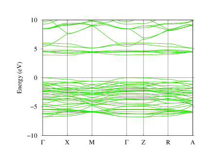
Fig. 11: Band structure of AFM KCoO₂ int he QS$GW$ approach.

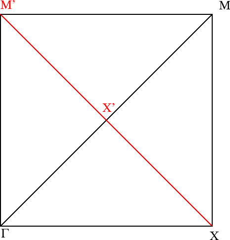
Fig. 12: Relation between primitive cell tetragonal Brillouin zone labeled in black and doubled cell 45 degree rotated Brillouin zone for AFM case, labeled in red and with primes.

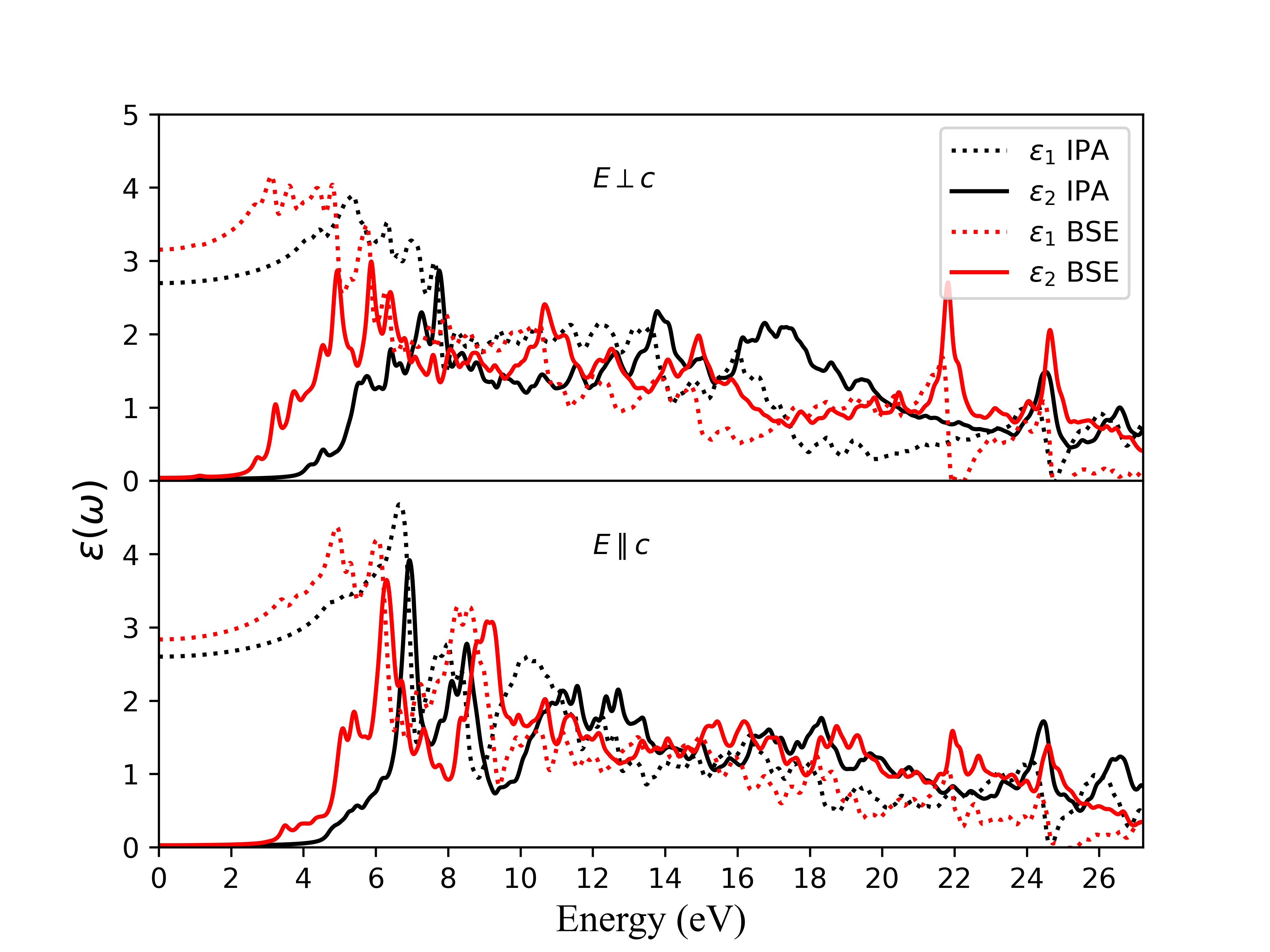
Fig. 13: Optical dielectric function for the AFM state.

The antiferromagnetic band structure is shown in Fig. 11. The relation between the FM primitive cell Brillouin zone and the AFM cell Brillouin zone is shown in Fig. 12. The new $\Gamma X$ direction is half the old $\Gamma M$ direction and the bands are essentially folded in two in that direction. The new $M$ point corresponds to the old $X$ point. The band structure now has a direct gap at $\Gamma$ of 3.94 eV because the spin up VBM state at $M$ becomes folded on the new $\Gamma$ state. Both the top valence and bottom conduction bands become almost entirely flat along $\Gamma Z$.

The optical dielectric function of the AFM state is shown in Fig. 13. It is calculated here using $N_{v}=48$ valence bands and $N_{c}=40$ conduction bands and a $3\times 3\times 3$ k-mesh. It is rather similar to the corresponding FM case shown in Fig. 8 although not quite identical. In both cases, we may note a substantial redshift between the IPA and BSE $\varepsilon_{2}(\omega)$ and excitonic features below the quasiparticle gap of 3.94 eV. We note that the sharp features for ${\bf E}\perp{\bf c}$ at 22 and 24 eV may be artifacts of the truncation of the active space in the BSE calculation. For a smaller set, similar features appeared for ${\bf E}\parallel{\bf c}$ around 15 eV but these disappear or are weakened when more conduction bands were included. The calculation may be deemed to be converged up to about 12 eV as in this range they are the same with higher or lower $N_{c}$.

IV Conclusions

The main conclusions from our study are summarized as follows. KCoO₂ has large magnetic moments of $4\mu_{B}$ on the Co atoms, corresponding to a $d_{xy}^{2}$, $d_{xz}^{1}$, $d_{yz}^{1}$, $d^{1}_{x^{2}-y^{2}}$, $d^{1}_{3z^{2}-r^{2}}$ configuration, arising from the square pyramidal coordination with a K ion on the opposing apical site. The magnetic moments prefer to order antiferromagnetically along the [110] direction. The exchange interactions are dominated by an antiferromagnetic super-exchange coupling between $d_{x^{2}-y^{2}}$ orbitals $\sigma$-bonding with O-$p$ orbitals between them in a 180^∘ alignment of order $\sim$8 meV but with smaller direct exchange between the two Co per primitive cell, thus aligning all spin on atoms in successive (110) planes. The Néel temperature was predicted to be about 100 K using the Tyablikov-Callen approach and using exchange interactions extracted from the transverse spin susceptibility in a rigid spin approximation per sphere and including a converged summation of exchange interactions. In the mean-field approximation, a larger critical temperature of about 250 K is obtained, which provides an upper limit. In the ferromagnetic state, the band structure exhibits an indirect gap between the conduction band minimum at $\Gamma$ of minority spin and a valence band maximum of majority spin at $M$, the corner of the Brillouin zone in the $k_{z}=0$ plane. The optical transitions between equal spin were calculated including electron-hole interaction effects and show strongly bound excitons. In the AFM case, the band edges of the gap show extremely flat regions along the direction perpendicular to the layers and a direct quasiparticle gap of 3.94 eV. The combination of large magnetic moments, relatively small exchange interactions of different types and flat band edge states indicate that strong correlation effects may be present in this system and could lead to interesting effects, in particular when doping is considered to modify the antiferromagnetic insulating ground state.