Abstract

Model-assisted, two-stage forest survey sampling designs provide a means to combine airborne remote sensing data, collected in a sampling mode, with field plot data to increase the precision of national forest inventory estimates, while maintaining important properties of design-based inventories, such as unbiased estimation and quantification of uncertainty. In this study, we present a comprehensive set of model-assisted estimators for domain-level attributes in a two-stage sampling design, including new estimators for densities, and compare the performance of these estimators with standard poststratified estimators. Simulation was used to assess the statistical properties (bias, variability) of these estimators, with both simple random and systematic sampling configurations, and indicated that 1) all estimators were generally unbiased. and 2) the use of lidar in a sampling mode increased the precision of the estimators at all assessed field sampling intensities, with particularly marked increases in precision at lower field sampling intensities. Variance estimators are generally unbiased for model-assisted estimators without poststratification, while model-assisted estimators with poststratification were increasingly biased as field sampling intensity decreased. In general, these results indicate that airborne remote sensing, collected in a sampling mode, can be used to increase the efficiency of national forest inventories.
Keywords: inventory, biomass, carbon, lidar, sampling.

1 Introduction

Reliable and credible information on forest status and change is needed to support effective natural resource management and policy. National forest inventory (NFI) programs are usually the primary source for this type of information, since, ideally, they are designed to provide accurate (unbiased) and precise estimates at regional and national scales. For example, NFI data is used to support global forest monitoring (FAO (2016)), national scale greenhouse gas monitoring (EPA (2023)), and emerging markets for trading of forest carbon offset credits (Marland et al. (2017)). The NFI is used to characterize various attributes (e.g., biomass, area) of the population for a multitude of domains (e.g., forest type), where estimates take the form of domain totals (e.g., total biomass of trees in forestland), areas (e.g., total forestland area), or per-unit-area densities (average tree biomass per hectare of forestland). A large network of field inventory plots are the basis for most NFI programs, and plots within homogeneous regions, or strata, are often grouped (and weighted by stratum area) to increase the precision of inventory estimates. Increasing interest in more accurate estimation across spatial scales ranging from smaller regions (e.g., county,parcel, or management unit) (Dettmann et al. (2022)) to vast, highly remote regions (tropical rainforests, high-latitude boreal forests), as well as other societal drivers such the need to verify forest carbon offset credits in carbon markets, has motivated the international forest monitoring community to more effectively leverage remote sensing in inventory sampling designs, including the use of high-resolution airborne remote sensing as an intermediate level of sampling in multi-stage sampling designs. In recent years, more advanced approaches to estimation have been proposed that can more fully leverage more sophisticated models and the rich information from both satellite and airborne remote sensing in the context of NFI programs (Ståhl et al. (2016); Lister et al. (2020); Kangas et al. (2018); McRoberts, Andersen, and Næsset (2014); Westfall et al. (2022)). For example, both model-assisted (Breidt and Opsomer (2017); McConville et al. (2017); Magnussen, Nord-Larsen, and Riis-Nielsen (2018)) and model-based techniques (McRoberts (2010)) have been developed to leverage wall-to-wall remote sensing data in forest inventory.

The use of high-resolution, airborne lidar strip sampling to support forest inventories has been the focus of several recent studies in Europe and North America where a variety of estimation approaches have been developed and evaluated, including model-assisted (Gregoire et al. (2011); Strunk et al. (2014); Ringvall et al. (2016)), model-based (Saarela et al. (2016)) and hybrid estimation (Ståhl et al. (2011); Ståhl et al. (2016)). Gobakken et al. (2012) compared several model-dependent and model-assisted estimators in a two-stage design using lidar sampling in the Hedmark region of Norway. Ringvall et al. (2016) developed a model-assisted estimator for two-stage lidar sample surveys that addressed several significant limitations of lidar sampling in the forest inventory context, including the use of a ratio estimator to account for varying strip lengths, and poststratification to further improve precision. This estimator has since been applied to repeat collections of lidar sampling data to support monitoring of forest change in Norway (Strîmbu et al. (2017)). In the context of the US NFI in interior Alaska, model-assisted (Andersen, Barrett, et al. (2009)), hierarchical Bayesian coregionalization model-based (Babcock et al. (2018)) and hybrid (Ene et al. (2018)) estimation approaches have been proposed as a means to combine information from NFI plots, a lidar strip sample, and wall-to-wall layers.

While these more complex sampling designs can often increase the efficiency of the inventory (higher precision at specified cost, or level of sampling effort), they often require the development of new estimators for inventory attributes, as well as new variance estimators to quantify uncertainty (i.e. variance) of the estimators. In particular, while approaches to classification (Andersen (2009); Shoot et al. (2021)) and estimation (McConville et al. (2017)) of domains in the NFI context have been recently investigated, no previous studies have developed ratio estimators for densities in a two-stage survey design framework. Assessing the statistical properties of these new estimators requires a simulation framework, where the true properties of the population are fixed and known and the sampling distributions of the estimators can be developed over many simulated samples. Assessment of the estimators via simulation is necessary to establish the reliability and defensibility of the estimators, especially in the context of a national forest inventory.

The objectives of this study are to present a set of model-assisted estimators for all types of NFI estimates required to report current status (domain totals, areas, and densities) that can incorporate three levels of information available in a poststratified, two-stage sampling design: (1) a sparse sample of field inventory plots, (2) a dense strip sample of airborne lidar, and (3) a wall-to-wall stratification layer. This comprehensive set of estimators includes those presented in previous studies (Ringvall et al. (2016)), as well as new ratio-of-ratios estimators for estimating densities.

2 Methods

2.1 Case study: Implementation of the National Forest Inventory in interior Alaska, USA

We focus on interior Alaska as an example of a region where an alternative sampling design, and corresponding estimators, are needed to support the NFI program. The US Forest Inventory and Analysis (FIA) program – the NFI for the United States – is mandated by the US Congress to assess current status and trends for all forest lands of the United States (USDA Forest Service (2016)). The standard sampling framework for FIA in the conterminous United States, coastal Alaska, and Pacific islands is a systematic, unaligned grid of field plots established with a sampling intensity of 1 plot per 2,428 ha. Interior Alaska is a vast region of high-latitude boreal forests (approx. 46 million hectares of forestland) with virtually no transportation infrastructure (virtually all plots are accessed via helicopter), and for this reason, FIA has implemented a modified sampling design in interior Alaska using a reduced sampling intensity for field plots (1 plot per 12,140 ha - 1/5^th the standard intensity – collected on a systematic grid), supplemented with high-resolution airborne imagery acquired by NASA Goddard’s Lidar, Hyperspectral, and Thermal (G-LiHT) Airborne Imager (Cook et al. (2013)) in a strip sampling mode (Cahoon and Baer (2022)) covering every FIA plot. The FIA field inventory of interior Alaska was initiated within the Tanana inventory unit (13.5 million ha) and carried out over a five-year period (2014-2018), and the G-LiHT collection was carried out in 2014 (see Figure 1).

Figure 1: Tanana inventory unit, interior Alaska, USA. Black lines indicate location of airborne G-LiHT flight lines. Dots indicate (approximate) location of FIA field plots (colored by biomass). Underlying raster indicates stratification, red outline indicates the domain sampled by G-LiHT.

2.2 Standard FIA sampling design and estimation

The sample-based estimators of population totals, areas, and densities (and corresponding variance estimators) used in standard FIA reporting assume that the plots are collected as a simple random sample (SRS), and the precision of these estimators is further improved through post-stratification, as documented in Bechtold and Patterson (2005). The poststrata used in FIA are generally developed based on available land cover maps, as well as ownership and other GIS layers.

2.2.1 Poststratified estimation of a domain total

Estimates of population totals, such as tree biomass, or carbon, are usually primary attributes of interest in a national forest inventory. In the standard estimation framework of FIA, these values are provided by the following estimators (including variance):

$${\overline{t}}_{h}=\frac{\sum_{i=1}^{n_{h}}y_{hi}}{n_{h}}$$ (1)

$${\widehat{t}}_{SRS,PS}=A_{T}\sum_{h=1}^{H}W_{h}{\overline{t}}_{h}$$ (2)

where $y_{hi}$ is the plot-level value (per ha) for an inventory attribute of interest (e.g., tree biomass, carbon, volume, etc.) on plot $i$ in stratum $h$, $n_{h}$ is the number of plots in stratum $h$, ($N_{h}$ is the size of the stratum in the population), $W_{h}=N_{h}/N$ is the weight for stratum $h$, and $A_{T}$ is the total area of the population (ha).

The variance estimator is:

$$\widehat{V}\left({\widehat{t}}_{SRS,PS}\right)=A_{T}^{2}\left[\sum_{h=1}^{H}W_{h}n_{h}\widehat{V}\left({\overline{t}}_{h}\right)+\sum_{h=1}^{H}\left(1-W_{h}\right)\frac{n_{h}}{n}\widehat{V}\left({\overline{t}}_{h}\right)\right]$$ (3)

$$\widehat{V}\left({\overline{t}}_{h}\right)=\frac{\sum_{i=1}^{n_{h}}y_{hi}^{2}-n_{h}{{\overline{t}}_{h}^{2}}}{n_{h}(n_{h}-1)}$$ (4)

2.2.2 Poststratified estimation of domain area

Estimation of domain area (e.g., total forestland area in hectares, etc.) is another primary output of a national forest inventory, and are provided by the following estimators (including variance):

$${\overline{a}}_{h}=\frac{\sum_{i=1}^{n_{h}}a_{hi}}{n_{h}}$$ (5)

$${\widehat{A}}_{SRS,PS}=A_{T}\sum_{h=1}^{H}W_{h}{\overline{a}}_{h}$$ (6)

where $a_{hi}$ is the proportion of plot $i$, in stratum $h$, within a given domain (e.g., forestland, forest type, etc.).

The variance estimator is:

$$\widehat{V}\left({\widehat{A}}_{SRS,PS}\right)=A_{T}^{2}\left[\sum_{h=1}^{H}W_{h}n_{h}\widehat{V}\left({\overline{a}}_{h}\right)+\sum_{h=1}^{H}\left(1-W_{h}\right)\frac{n_{h}}{n}\widehat{V}\left({\overline{a}}_{h}\right)\right]$$ (7)

$$\widehat{V}\left({\overline{a}}_{h}\right)=\frac{\sum_{i=1}^{n_{h}}a_{hi}^{2}-n_{h}{\overline{a}}_{h}^{2}}{n_{h}(n_{h}-1)}$$ (8)

2.2.3 Poststratified estimation of a domain density

The final category of estimates required in a NFI include densities for various inventory attributes on a per-unit-area basis. In the case where a density is estimated over the entire area of the population, the estimator is obtained by simply dividing the estimator of the total $\widehat{t}_{SRS,PS}$ by the known area of the population $A_{T}$, and the corresponding variance estimator is obtained by dividing the variance of the total by $A_{T}^{2}$. However, often a density is estimated for a domain (e.g., tree carbon per forested hectare, where the domain is forestland). Because both the numerator and denominator of these estimators are themselves estimators, they are considered $ratio$ estimators. The poststratified estimator of domain density used in FIA is given by:

$${\widehat{D}}_{SRS,PS}=\frac{\sum_{h=1}^{H}W_{h}{\overline{t}}_{h}}{\sum_{h=1}^{H}W_{h}{\overline{a}}_{h}}$$ (9)

with variance estimator:

$$\widehat{V}\left({\widehat{D}}_{SRS,PS}\right)=\frac{1}{{\widehat{A}}_{SRS,PS}^{2}}\left[\widehat{V}\left({\widehat{t}}_{SRS,PS})+{\widehat{D}}_{SRS,PS}^{2}{\widehat{V}(\widehat{A}}_{SRS,PS})\right)-2{\widehat{D}}_{SRS,PS}\ Cov\left({\widehat{t}}_{SRS,PS},{\widehat{A}}_{SRS,PS}\right)\right]$$ (10)

where

$$Cov\left({\widehat{t}}_{SRS,PS},{\widehat{A}}_{SRS,PS}\right)=\frac{A_{T}^{2}}{n}\left[\sum_{h=1}^{H}W_{h}n_{h}Cov\left({\overline{t}}_{h},{\overline{a}}_{h}\right)+\sum_{h=1}^{H}\left(1-W_{h}\right)\frac{n_{h}}{n}Cov\left({\overline{t}}_{h},{\overline{a}}_{h}\right)\right]$$ (11)

$$Cov\left({\overline{t}}_{h},{\overline{a}}_{h}\right)=\frac{\sum_{i=1}^{n_{h}}y_{hi}a_{hi}-n_{h}{\overline{t}}_{h}{\overline{a}}_{h}}{n_{h}\left(n_{h}-1\right)}$$ (12)

2.3 Ratio estimators for model-assisted estimation in two-stage sampling designs

2.3.1 Sampling design and notation

The addition of another level of sampling, e.g., provided by high-resolution, airborne data, collected as a strip sample, requires a different set of domain-level estimators. The notation and formulas used to describe these estimators mainly follow the notation and formulas used by Ringvall et al. (2016). The study area is partitioned into M non-overlapping strips, denoted as PSUs. These strips have unequal lengths and thus unequal areas, and the set U₁ is the population of PSUs. A first-stage sample, S₁, of PSUs is selected. Each PSU is partitioned into N_i grid-cells (SSUs) with a size roughly corresponding to the size of the field plots. In the second stage, we randomly select a sample S_i of SSUs from each PSU. Subsampling within selected PSUs are invariant of which PSUs are selected in the first stage. The total number of grid-cells in the study area is $N=\sum_{i\in U_{1}}N_{i}$.

In inventory programs where the plot is actually a cluster of several subplots (as is the case with many NFIs, including FIA), a slight adjustment to the sampling framework can be used to maintain consistency in the spatial support (i.e. plot footprint) for sampling units at the different sampling stages. To this end, in this study N is the number of points on the 200 meter hexagonal grid across the study area, $N_{i}$ is the points on this grid along the $i^{th}$ PSU. The per-ha average is estimated for each attribute in N and then scaled up to the level of the population by multiplying by the population area, $A_{T}$. However, for the purposes of clarity and consistency, we maintain the more general notation used in Ringvall et al. (2016) in the following sections (it should be noted that the above adjustment does not change the results).

Several other details regarding the sampling design should be noted. First, in practice lidar strips are often allocated systematically, traversing the entire area of study, but we assume them to be randomly allocated from the point of view of the variance formulas. Likewise, field plots are often distributed systematically (i.e. at a regular spacing) within lidar strips, we assume them to be randomly allocated within strips, at a specified sampling intensity, from the point of view of the variance formulas. As is the case with many standard NFI designs, the entire study area is divided into strata, and this map information is incorporated in the estimators through poststratification. It should also be noted that the lidar strip sampling is carried out independent of the stratification. In addition, the strata normally do not coincide with the domains of interest, since areas belonging to the domain potentially appear scattered across several strata and they cannot be perfectly identified on maps, but only in the field on the subplots. Prediction models for the variable of interest (e.g., biomass per ha), as well as the domain (e.g., forestland), are developed from the collected field data.

2.3.2 A ratio estimator of the domain total

With simple random sampling without replacement in both stages, a ratio (R) estimator of the variable of interest within a given domain (cf. Ringvall et al. (2016), eq. 5) is

$$\widehat{t}_{R}=N\frac{\sum_{i=1}^{m}{\ {\widehat{t}}_{ri}}}{\sum_{i=1}^{m}N_{i}}$$ (13)

where m is the number of selected PSUs and ${\widehat{t}}_{ri}$ is the model-assisted estimator of total biomass in a given domain (where the r subscript denotes a regression estimator) in the $i^{th}$ PSU given as

$$\widehat{t}_{ri}=\sum_{k=1}^{N_{i}}{{\widehat{q}}_{k}{\widehat{y}}_{k}}+\frac{N_{i}}{n_{i}}\sum_{k=1}^{n_{i}}e_{k}$$ (14)

where n_i is the number of selected SSUs within PSU i, ${\widehat{y}}_{k}$ is a predicted value of the domain-level attribute of interest based on a regression (or similar) model within a grid cell/plot, $\widehat{q}_{k}$ is an indicator variable (e.g., based on logistic regression) predicting whether or not the grid cell/plot belongs to the domain (or a prediction of the proportion in a domain, e.g., Van den Boogaart and Tolosana-Delgado (2013)), and $e_{k}$ is a deviation between the measured and predicted plot-level value for the variable of interest in the domain. In cases where the domain membership is incorporated into the regression model predicting the variable of interest (e.g., biomass is always zero on “nonforest” plots), the $\widehat{q}_{k}$ term can be omitted. It should be noted that predictions of the target variable and domain membership are made at the scale of the entire plot. If predictions are made at subplot scale in the case of cluster plots, it is assumed that these predictions, and associated error terms, are averaged and aggregated to the plot scale.

The variance estimator of ${\widehat{t}}_{R}$ is

$$\widehat{V}\left({\widehat{t}}_{R}\right)=\frac{N^{2}}{{\widehat{N}}^{2}}\left[M^{2}\left(\frac{1}{m}-\frac{1}{M}\right)s_{r}^{2}+\frac{M}{m}\sum_{S_{1}}N_{i}^{2}\left(\frac{1}{n_{i}}-\frac{1}{N_{i}}\right)s_{e}^{2}\right]$$ (15)

where $s_{r}^{2}=\frac{1}{m-1}\sum_{i=1}^{m}{({\widehat{t}}_{ri}-\widehat{R}N_{i})}^{2}$ with $\widehat{R}=\frac{\sum_{i=1}^{m}{\ {\widehat{t}}_{ri}}}{\sum_{i=1}^{m}N_{i}}$ and $s_{e}^{2}=\frac{1}{n_{i}-1}\sum_{k=1}^{n_{i}}\left(e_{k}-{\overline{e}}_{i}\right)^{2}$ with ${\overline{e}}_{i}=\frac{1}{n_{i}}\sum_{k=1}^{n_{i}}e_{k}$.

2.3.3 A ratio estimator of the domain total in poststratified estimation

When m PSUs are selected with simple random sampling without replacement in the first stage and n_i units are selected with simple random sampling with replacement in the second stage (as before), an estimator of a stratum total is

$$\widehat{t}_{Rh}=N_{h}\frac{\sum_{i=1}^{m}{\widehat{t}}_{rhi}}{\sum_{i=1}^{m}N_{hi}}$$ (16)

with

$$\widehat{t}_{rhi}=\sum_{k=1}^{N_{hi}}{{\widehat{q}}_{hk}{\widehat{y}}_{hk}}+\frac{N_{hi}}{n_{hi}}\sum_{k=1}^{n_{hi}}e_{hk}$$ (17)

where the notation follows from the previously used notation, but refers to a specific stratum h. Note that $e_{hk}$ involves either (1) prediction of domain membership for subplots and averaging across subplots, or (2) prediction of domain membership for the entire plot. In addition, all subplots are assumed to belong to the same stratum.

The poststratified estimator of the domain total is:

$${\widehat{t}}_{R,PS}=\sum_{h=1}^{H}{\widehat{t}}_{Rh}$$ (18)

The variance estimator becomes (from Ringvall et al. (2016))

$$\widehat{V}({\widehat{t}}_{Rh})=\left(\frac{N_{h}}{{\widehat{N}}_{h}}\right)^{2}\left(M^{2}\left(\frac{1}{m}-\frac{1}{M}\right)s_{rh}^{2}+\frac{M}{m}\sum_{S_{1}}{{\widehat{V}(\widehat{t}}_{rhi})}\right)$$ (19)

where $s_{rh}^{2}=\frac{1}{m-1}\sum_{i=1}^{m}\left({\widehat{t}}_{rhi}-{\widehat{R}}_{h}N_{hi}\right)^{2}$ with ${\widehat{R}}_{h}=\frac{\sum_{S_{I}}{\widehat{t}}_{rhi}}{\sum_{S_{I}}N_{hi}}$. The within PSU variance $V({\widehat{t}}_{rhi})$ is estimated as

$$\widehat{V}(\widehat{t}_{rhi})=N_{hi}^{2}\left(\frac{1}{n_{hi}}-\frac{1}{N_{hi}}\right)s_{{\widehat{e}}_{hi}}^{2}$$ (20)

with $s_{e,h}^{2}=\frac{1}{n_{hi}-1}\sum_{k=1}^{n_{hi}}{({e_{hk}-{\overline{e}}_{hi})}^{2}}$ and ${\overline{e}}_{hi}=\frac{1}{n_{hi}}\sum_{k=1}^{n_{hi}}e_{hk}$.

Finally, the poststratified estimator of the domain total is ${\widehat{t}}_{R,PS}=\sum_{h=1}^{H}{N_{h}\frac{\sum_{i=1}^{m}{\widehat{t}}_{rhi}}{\sum_{i=1}^{m}N_{hi}}}$. The variance estimator is

$$\widehat{V}\left({\widehat{t}}_{R,PS}\right)=\sum_{h=1}^{H}{{\widehat{V}(\widehat{t}}_{Rh})+\sum_{h=1}^{H}{\sum_{g\neq h}{\frac{N_{h}}{{\widehat{N}}_{h}}\frac{N_{g}}{{\widehat{N}}_{g}}M^{2}\left(\frac{1}{m}-\frac{1}{M}\right)\frac{\sum_{i=1}^{m}\left(\left({\ \widehat{t}}_{rhi}-{\widehat{R}}_{h}N_{hi}\right)\left({\ \widehat{t}}_{rgi}-{\widehat{R}}_{g}N_{gi}\right)\right)}{m-1}}}}$$ (21)

with ${\widehat{V}(\widehat{t}}_{Rh})$ given by Eq. 19. In this case the computations can be limited to those strata where the domain has a potential to occur. Note that because in our case sampling in not conducted independently between strata, the variance estimator (Eq. 21) must account for covariances among strata (i.e. the last term on the right hand side).

2.3.4 A ratio estimator of the domain area

So far, the population total within the domain has been addressed. Following the previous notation and estimation principles, a domain area estimator (without poststratification) would be

$$\widehat{A}_{R}=N\frac{\sum_{i=1}^{m}{\ {\widehat{a}}_{ri}}}{\sum_{i=1}^{m}N_{i}}$$ (22)

where ${\widehat{a}}_{ri}$ is the model-assisted estimator of total domain area in the $i^{th}$ PSU given as

$$\widehat{a}_{ri}=\sum_{k=1}^{N_{i}}{{\widehat{q}}_{k}\ a\_cell}+\frac{N_{i}}{n_{i}}\sum_{k=1}^{n_{i}}e_{k}$$ (23)

where $a\_cell$ is the area of a grid-cell. The other notation is the same as previously, and notably $e_{k}$ is a deviation between a measured and predicted plot/grid-cell level value for the proportion of the plot within the domain. Like for the target variable of interest, $e_{k}$ should be the aggregated and averaged difference across subplots, recalculated to correspond to the size of a grid-cell.

The variance estimator of ${\widehat{A}}_{R}$ is

$$\widehat{V}\left({\widehat{A}}_{R}\right)=\frac{N^{2}}{{\widehat{N}}^{2}}\left[M^{2}\left(\frac{1}{m}-\frac{1}{M}\right)s_{r}^{2}+\frac{M}{m}\sum_{S_{1}}N_{i}^{2}\left(\frac{1}{n_{i}}-\frac{1}{N_{i}}\right)s_{e}^{2}\right]$$ (24)

where $s_{r}^{2}=\frac{1}{m-1}\sum_{i=1}^{m}{({\widehat{a}}_{ri}-\widehat{R}N_{i})}^{2}$ with $\widehat{R}=\frac{\sum_{i=1}^{m}{\ {\widehat{a}}_{ri}}}{\sum_{i=1}^{m}N_{i}}$ and $s_{e}^{2}=\frac{1}{n_{i}-1}\sum_{k=1}^{n_{i}}\left(e_{k}-{\overline{e}}_{i}\right)^{2}$ with ${\overline{e}}_{i}=\frac{1}{n_{i}}\sum_{k=1}^{n_{i}}e_{k}$..

2.3.5 A ratio estimator of the domain area in poststratified estimation

So far, the population total within the domain has been addressed. Following the previous notation and estimation principles, a domain area estimator (with poststratification) would be

$$\widehat{A}_{Rh}=N_{h}\frac{\sum_{i=1}^{m}{\widehat{a}}_{rhi}}{\sum_{i=1}^{m}N_{ih}}$$ (25)

where ${\widehat{a}}_{rhi}$ is the model-assisted estimator of total domain area, in stratum h, in the $i^{th}$ PSU given as

$$\widehat{a}_{rhi}=\sum_{k=1}^{N_{hi}}{{\widehat{q}}_{hk}\ a\_cell}+\frac{N_{hi}}{n_{hi}}\sum_{k=1}^{n_{hi}}e_{hk}$$ (26)

where $a\_cell$ is the area of a grid-cell.

The poststratified estimator of the total population area is:

$${\widehat{A}}_{R,PS}=\sum_{h=1}^{H}{\widehat{A}}_{Rh}$$ (27)

with variance estimator

$$\widehat{V}\left({\widehat{A}}_{Rh}\right)=\left(\frac{N_{h}}{{\widehat{N}}_{h}}\right)^{2}\left(M^{2}\left(\frac{1}{m}-\frac{1}{M}\right)s_{rh}^{2}+\frac{M}{m}\sum_{S_{1}}{{\widehat{V}(\widehat{a}}_{rhi})}\right)$$ (28)

where $s_{rh}^{2}=\frac{1}{m-1}\sum_{i=1}^{m}\left({\widehat{a}}_{rhi}-{\widehat{R}}_{a,h}N_{hi}\right)^{2}$ and ${\widehat{R}}_{a,h}=\frac{\sum_{S_{1}}{\widehat{a}}_{rhi}}{\sum_{S_{1}}N_{hi}}$. $V({\widehat{t}}_{rhi})$is estimated as

$$\widehat{V}(\widehat{a}_{rhi})=N_{hi}^{2}\left(\frac{1}{n_{hi}}-\frac{1}{{\widehat{N}}_{hi}}\right)s_{e,h}^{2}$$ (29)

with $s_{e,h}^{2}=\frac{1}{n_{hi}-1}\sum_{k=1}^{n_{hi}}{({e_{hk}-{\overline{e}}_{hi})}^{2}}$ and ${\overline{e}}_{hi}=\frac{1}{n_{hi}}\sum_{k=1}^{n_{hi}}e_{hk}$.

A variance estimator for the total domain area is given by:

$$\widehat{V}\left({\widehat{A}}_{R,PS}\right)=\sum_{h=1}^{H}{{\widehat{V}(\widehat{A}}_{Rh})+\sum_{h=1}^{H}{\sum_{g\neq h}{\frac{N_{h}}{{\widehat{N}}_{h}}\frac{N_{g}}{{\widehat{N}}_{g}}M^{2}\left(\frac{1}{m}-\frac{1}{M}\right)\frac{\sum_{i=1}^{m}\left(\left({\ \widehat{a}}_{rhi}-{\widehat{R}}_{a,h}N_{hi}\right)\left({\ \widehat{a}}_{rgi}-{\widehat{R}}_{a,g}N_{gi}\right)\right)}{m-1}}}}$$ (30)

with ${\widehat{V}(\widehat{A}}_{Rh})$ given by Eq. 27.

2.3.6 A ratio-of-ratios estimator of the domain density

In the context of forest inventory, we are often also interested in domain densities, in addition to domain totals and areas. Because the form of the estimator of domain density is a ratio estimator, where the numerator and denominator are themselves ratio estimators, we term the form of this new estimator as a ratio-of-ratios, or RoR, estimator.

$$\widehat{D}_{RoR}=\frac{{\widehat{t}}_{R}}{{\widehat{A}}_{R}}=\ \frac{N\frac{\sum_{i=1}^{m}{\ {\widehat{t}}_{ir}}}{\sum_{i=1}^{m}N_{i}}}{N\frac{\sum_{i=1}^{m}{\ {\widehat{a}}_{ir}}}{\sum_{i=1}^{m}N_{i}}}=\frac{\sum_{i=1}^{m}{\ {\widehat{t}}_{ir}}}{\sum_{i=1}^{m}{\widehat{a}}_{ir}}$$ (31)

where ${\widehat{t}}_{R}$ is the ratio domain biomass estimator and ${\widehat{A}}_{R}$ is the ratio domain area estimator. Introducing the new variables $u_{i}=$ ${\widehat{t}}_{i}-{\widehat{D}}_{RoR}{\widehat{a}}_{i}$ and $v_{ik}=e_{ik}^{y}-{\widehat{D}}_{RoR}{\widehat{a}}_{ik}$ the variance estimator for ${\widehat{D}}_{RoR}$ is

$$\widehat{V}\left({\widehat{D}}_{RoR}\right)=\frac{1}{\widehat{A^{*}}^{2}}\left[M^{2}\left(\frac{1}{m}-\frac{1}{M}\right)s_{u}^{2}+\frac{M}{m}\sum_{S_{1}}N_{i}^{2}\left(\frac{1}{n_{i}}-\frac{1}{N_{i}}\right)s_{vi}^{2}\right]$$ (32)

where $s_{u}^{2}=\frac{1}{m-1}\sum_{i=1}^{m}{({u}_{i}-\overline{u})}^{2}$, $s_{vi}^{2}=\frac{1}{n_{i}-1}\sum_{k=1}^{n_{i}}\left({v}_{ik}-\overline{v}_{i}\right)^{2}$, and the term $\widehat{A^{*}}$ is computed as the average estimated area from the sampled strips, times the total number of strips in the population, M. Details regarding the derivation of $\widehat{V}\left({\widehat{D}}_{RoR}\right)$ are provided in Appendix A.

2.3.7 A ratio-of-ratios estimator of the domain density with poststratification

The ratio-of-ratios estimator takes on a more complex form in a poststratified (or prestratified) setting, since in the case of poststratification we must account for dependencies (i.e. covariance) between the estimators for different strata, since a single survey line may cross over several strata.

The ratio-of-ratios estimator with poststratification is:

$$\widehat{D}_{RoR,PS}=\frac{{\widehat{t}}_{R,PS}}{{\widehat{A}}_{R,PS}}=\frac{\sum_{h}{\widehat{t}}_{Rh}}{\sum_{h}{\widehat{A}}_{Rh}}=\ \frac{\sum_{h}{N_{h}\frac{\sum_{i=1}^{m}{\ {\widehat{t}}_{rhi}}}{\sum_{i=1}^{m}N_{hi}}}}{\sum_{h}{N_{h}\frac{\sum_{i=1}^{m}{\ {\widehat{a}}_{rhi}}}{\sum_{i=1}^{m}N_{hi}}}}$$ (33)

Note that summation in (33) is across all sample strips, even if a stratum is not present in that strip. In such cases, the contribution from the strip is zero. Alternatively, (see Ringvall et al. (2016)) an estimator could be based on summation only across those strips that contain the stratum, in which case the basic estimator (33) would remain the same but the variance and variance estimators would be slightly different. In the following, the variances are developed for the case of summation across all strips.

Details related to the derivation of the variance estimator of $\widehat{D}_{RoR,PS}$ are provided in Appendix B, which results in the following:

$$\widehat{V}\left({\widehat{D}}_{RoR,PS}\right)\approx\frac{1}{{\widehat{A}}_{R,PS}^{2}}\widehat{V}\left({\widehat{t}}_{R,PS}-{\widehat{D}}_{RoR,PS}{\widehat{A}}_{R,PS}\right)=\\ \frac{1}{{\widehat{A}}_{R,PS}^{2}}\left[\widehat{V}\left({\widehat{t}}_{R,PS})+{\widehat{D}}_{RoR,PS}^{2}{\widehat{V}(\widehat{A}}_{R,PS})\right)-2{\widehat{D}}_{RoR,PS}\ \widehat{Cov}\left({\widehat{t}}_{R,PS},{\widehat{A}}_{R,PS}\right)\right]$$ (34)

with

$$\widehat{V}\left({\widehat{t}}_{R,PS}\right)=\sum_{h}{\ \frac{N_{h}^{2}}{{\widehat{N}}_{h}^{2}}\left[M^{2}\left(\frac{1}{m}-\frac{1}{M}\right)s_{rh}^{2}+\frac{M}{m}\sum_{S1}N_{hi}^{2}\left(\frac{1}{n_{hi}}-\frac{1}{N_{hi}}\right)s_{e,h}^{2}\right]}+\\ \sum_{h}{\sum_{g\neq h}{\frac{N_{h}N_{g}}{{\widehat{N}}_{h}{\widehat{N}}_{g}}M^{2}\left(\frac{1}{m}-\frac{1}{M}\right)\widehat{Cov}\left(r_{h},r_{g}\right)\ }}$$ (35)

and

$${\widehat{V}(\widehat{A}}_{R,PS})=\sum_{h}{\frac{N_{h}^{2}}{{\widehat{N}}_{h}^{2}}\left[M^{2}\left(\frac{1}{m}-\frac{1}{M}\right)s_{ra,h}^{2}+\frac{M}{m}\sum_{S1}N_{hi}^{2}\left(\frac{1}{n_{hi}}-\frac{1}{N_{hi}}\right)s_{ea,h}^{2}\right]}+\\ \sum_{h}{\sum_{g\neq h}{\frac{N_{h}N_{g}}{{\widehat{N}}_{h}{\widehat{N}}_{g}}M^{2}\left(\frac{1}{m}-\frac{1}{M}\right)\widehat{Cov}\left(r_{a,h},r_{a,g}\right)\ }}$$ (36)

and

$$\widehat{Cov}\left({\widehat{t}}_{R,PS},{\widehat{A}}_{R,PS}\right)=\sum_{h}{\sum_{g}{\frac{N_{h}N_{g}}{{\widehat{N}}_{h}{\widehat{N}}_{g}}M^{2}\left(\frac{1}{m}-\frac{1}{M}\right)\widehat{Cov}\left(r_{h},r_{a,g}\right)}}$$ (37)

where $r_{h}={\widehat{t}}_{rhi}-{\widehat{R}}_{h}N_{hi}$ and $r_{a,h}={\widehat{a}}_{rhi}-{\widehat{R}}_{a,h}N_{hi}$, and the covariance terms estimated in the usual way across the $m$ survey strips.

3 Evaluation

3.1 Empirical material and artificial population

3.1.1 FIA field plot measurements

The standard FIA plot is made up of four 1/60^th ha (7.3 m radius) fixed-area, circular subplots spaced 36.6 meters apart (for details on the FIA plot design and measurements, see Cahoon and Baer (2022)).The coordinates of each subplot were obtained (with less than 2 meters error) with GLONASS-enabled Trimble GeoXH mapping-grade GNSS receivers (McGaughey et al. (2017); Andersen, Clarkin, et al. (2009); Andersen, Strunk, and McGaughey (2022)). Aboveground dry biomass (Mg) for each measured tree was calculated using standard FIA procedures, and aggregated at the plot level (Mg/ha). In addition, the proportion of the FIA plot classified as accessible forestland was recorded as a fractional value between 0 and 1 (inclusive).

3.1.2 G-LiHT airborne laser scanning sampling

To augment the relatively sparse sample of field plots, single, linear swaths of high-resolution airborne remote sensing measurements, placed approximately 9.2 km apart, oriented in a NW-SW direction and covering every FIA plot, were acquired using G-LiHT mounted on a fixed-wing (Piper Cherokee) platform (Cook et al. (2013)) (see Figure 1). In this study, only the airborne lidar data from the G-LiHT instrument was utilized. The specifications for the lidar data collection are provided in Table 1.

Table 1: G-LiHT lidar specifications

Instrument	Riegl VQ-480
Laser wavelength	1550 nm
Flying height	335 m AGL
Beam divergence	0.3 mrad
Footprint size	10 cm
Half-scanning angle	15 degrees
Average pulse density	3 pulses/m2
Swath width	400 m

Lidar point cloud data was processed into 1 m resolution Digital Terrain and Canopy Height Models (DTM and CHM, respectively) for actual measured and simulated FIA field plots (1/15^th ha each) spaced 200 m apart on G-LiHT transects, resulting in a total of 59,090 total remote sensing plots (Figure 1). In order to allow for a direct comparison between high-resolution lidar-based canopy heights and the field-measured FIA inventory parameter (e.g., tree biomass), and to avoid any bias or inefficiency due to a difference in spatial support regions between the FIA plot footprint and the airborne lidar measurements, in this study the lidar was extracted within a discrete number of “remote sensing plots” corresponding exactly to the FIA plot footprint (i.e. four 1/60^th ha subplots, etc.), and spaced at 200 meter intervals along the center of the G-LiHT swaths. The approach resulted in 73,509 total remote sensing plots within the Tanana G-LIHT coverage(Figure 1) , the average of the lidar CHM grid-cells within a FIA plot footprint (1/15^th ha) was calculated for (1) each actual field-measured FIA plot, and (2) remote sensing plots distributed over the entire lidar coverage area.

3.1.3 Stratification layer

A stratification layer was generated from the National Land Cover Database (Homer et al. (2015)) by reclassifying “Evergreen Forest” (Class 42) as Class 1, “Mixed Forest” (class 43) as class 2, “Deciduous Forest” (class 41) as Class 3, and all other classes as Class 0. These strata were chosen so that stratum was an ordinal variable and biomass has a positive correlation with stratum, a desirable feature in developing the simulated population (described in next section).

3.1.4 Artificial population

Simulation can be a useful approach to gain insight into the statistical properties of various survey estimators, especially in the case of somewhat complex, multi-level sampling designs(Ene et al. (2012); Saarela et al. (2017)). When generating a simulated environmental population, it is desirable to include realistic correlations between the response variable (e.g., biomass, forest type, etc.) and the predictor variables used in the estimator (e.g., lidar height, strata, etc.), realistic marginal distributions for the attributes, and realistic spatial variation across multiple scales.

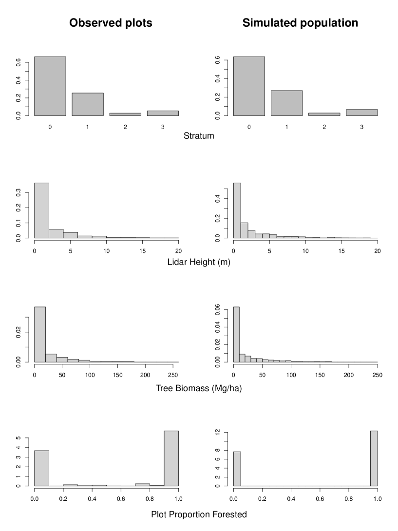
Figure 2: Marginal distributions from Observed Plots (left column) and Simulated Population (right column).

Table 2: Correlation Matrices for a) Observed field data, and b) Simulated population

(a)

	Stratum	Lidar Ht.	$y$	$a$
Stratum	1.00	0.64	0.58	0.41
Lidar Ht.	0.64	1.00	0.89	0.42
$y$	0.58	0.89	1.00	0.42
$a$	0.41	0.42	0.42	1.00

(b)

	Stratum	Lidar Ht.	$y$	$a$
Stratum	1.00	0.53	0.60	0.28
Lidar Ht.	0.53	1.00	0.84	0.42
$y$	0.60	0.84	1.00	0.37
$a$	0.28	0.42	0.37	1.00

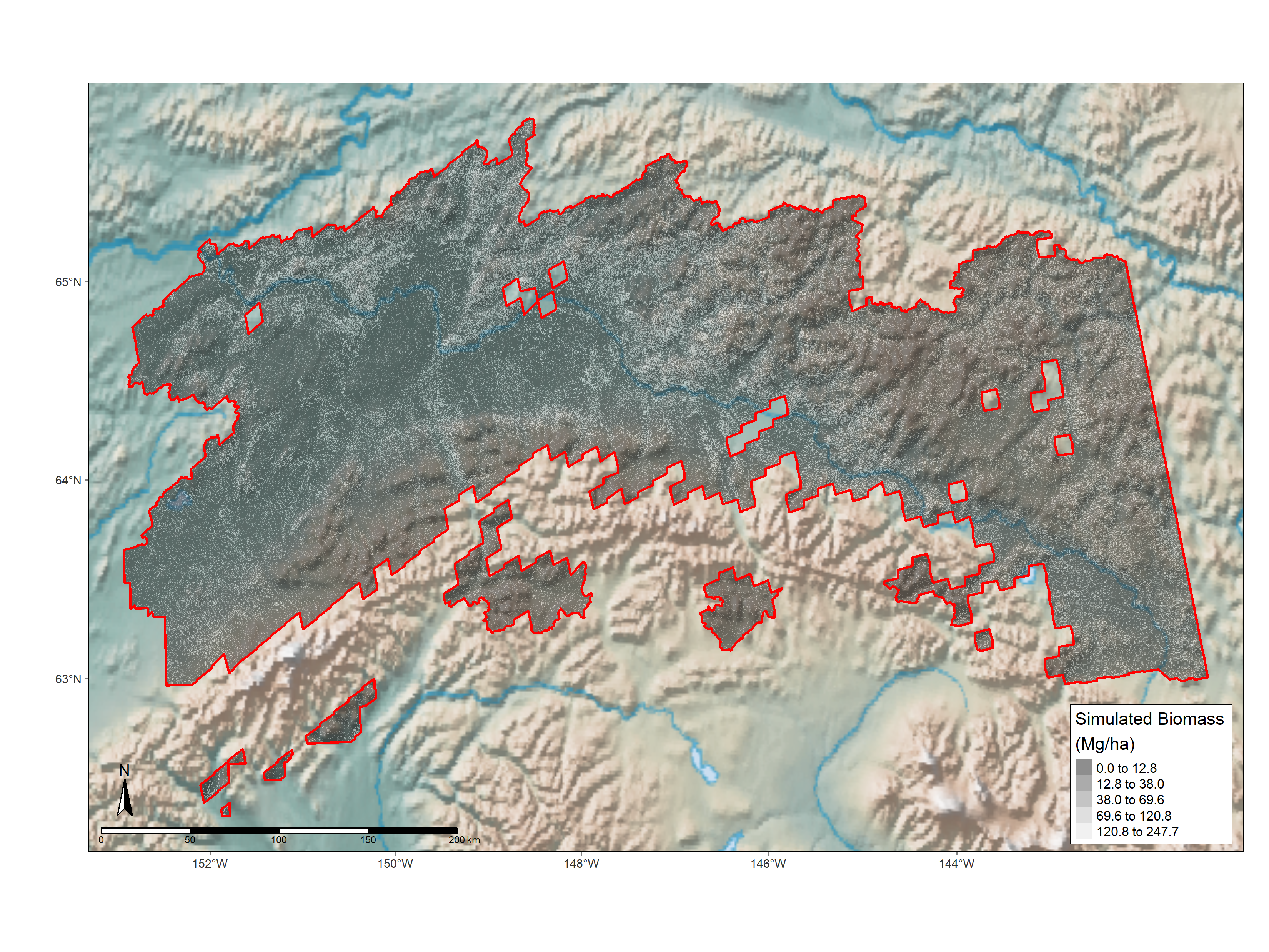
Figure 3: Spatial distribution of simulated population within Tanana study area

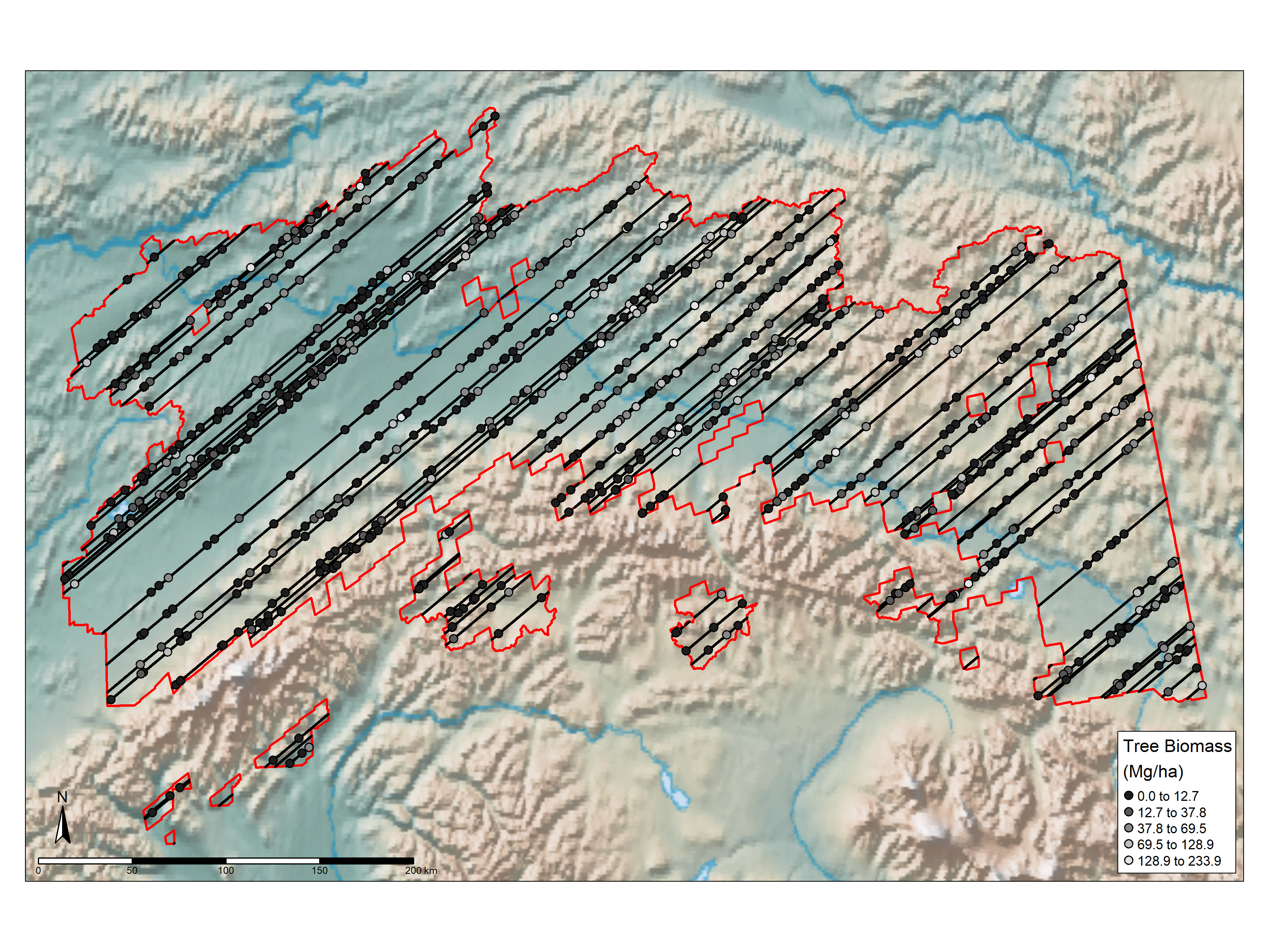
(a) Field plot sampling intensity: 0.015

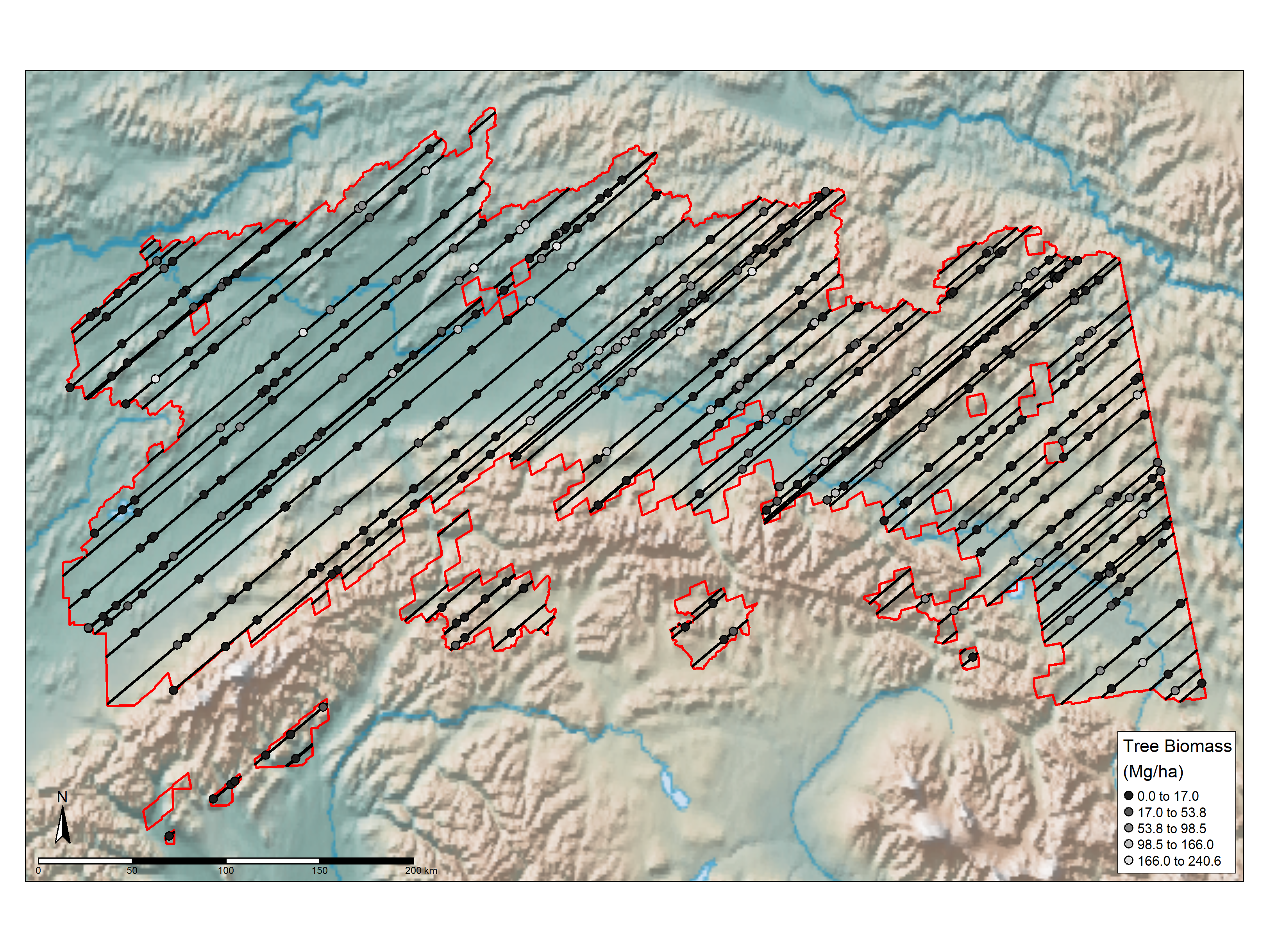
(b) Field plot sampling intensity: 0.0075

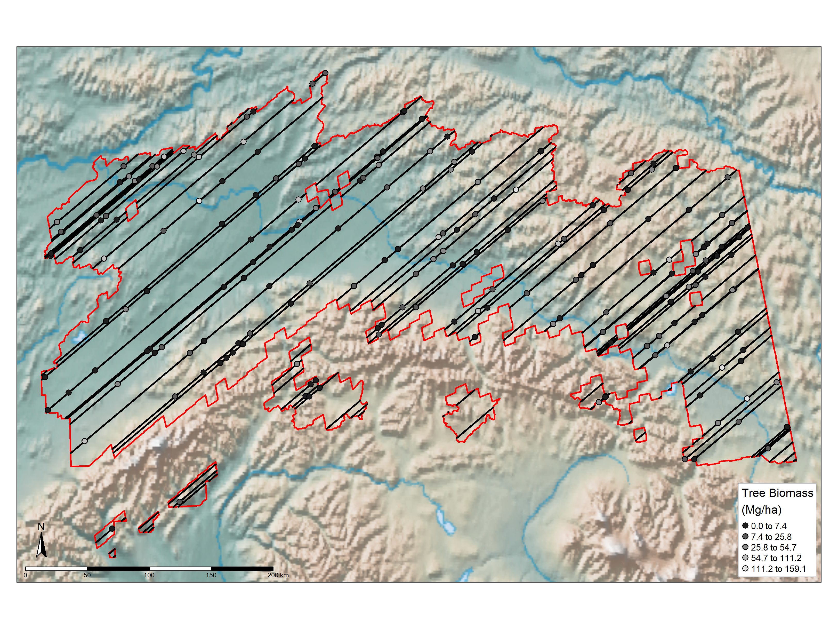
(c) Field plot sampling intensity: 0.00375

Figure 4: Simulated samples at different sampling intensities with simple random sampling. Black lines indicate random sampled of airborne lidar flight lines. Dots indicate simulated field plots, color-coded by biomass

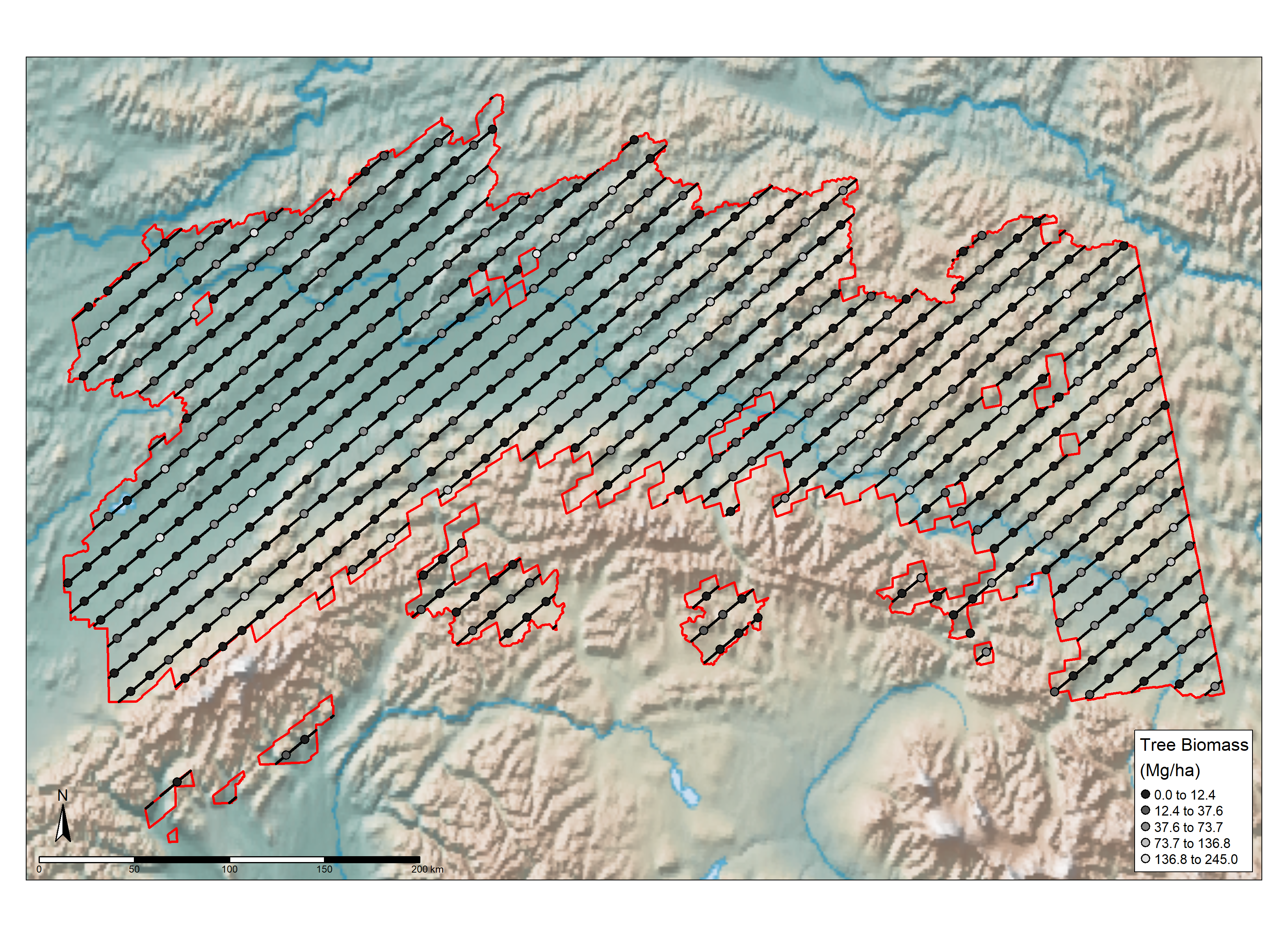
(a) Field plot sampling intensity: 0.015

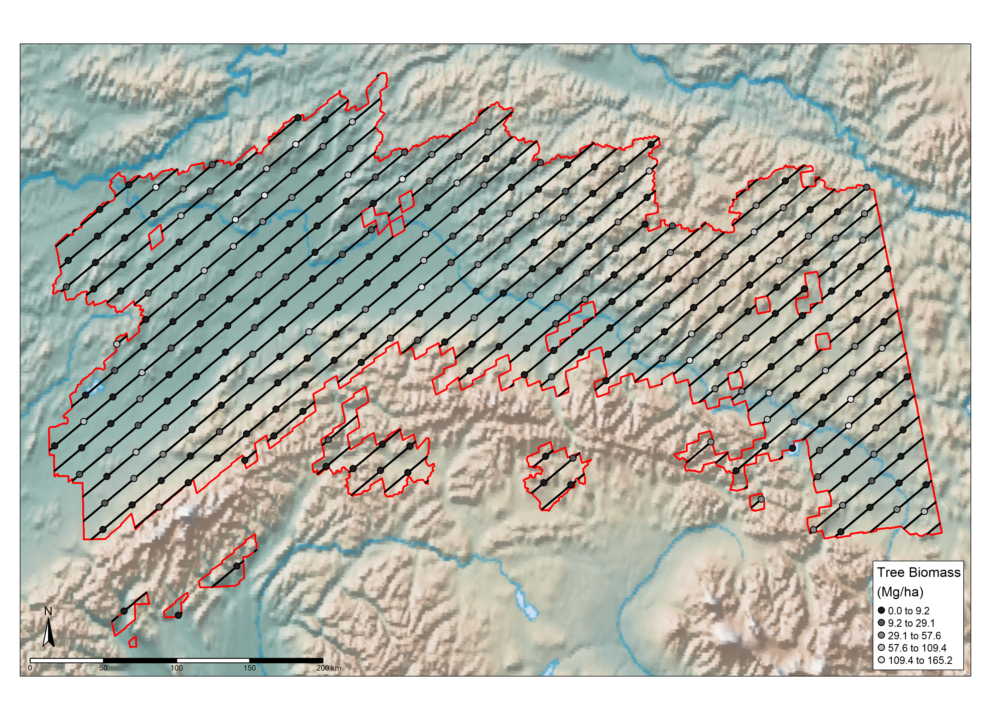
(b) Field plot sampling intensity: 0.0075

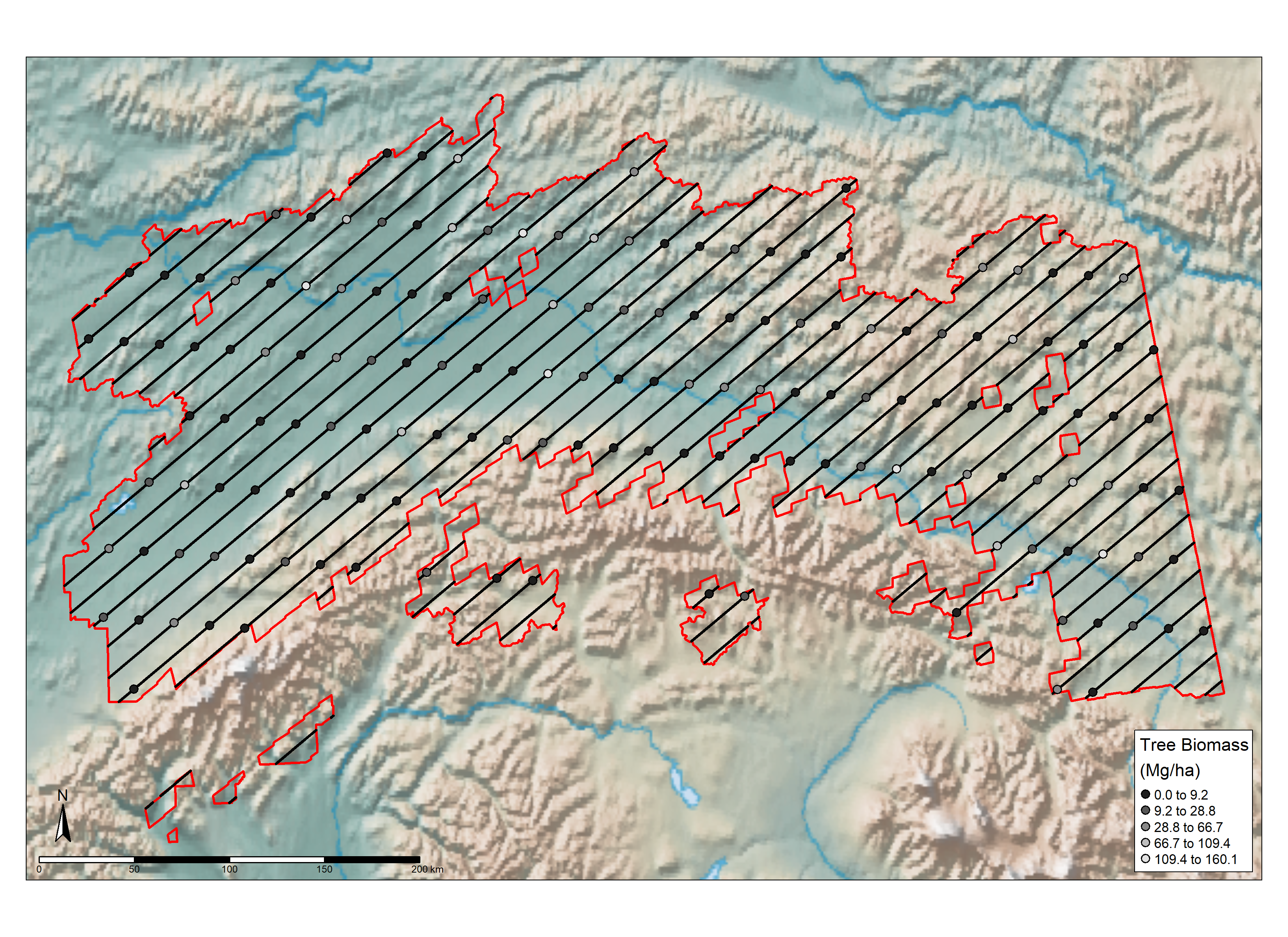
(c) Field plot sampling intensity: 0.00375

Figure 5: Simulated samples at different sampling intensities with systematic sampling. Black lines indicate random sampled of airborne lidar flight lines. Dots indicate simulated field plots, color-coded by biomass

In this study, we use a combination of modeling approaches and nearest-neighbor imputation to develop a simulated population over the Tanana study area, with the objectives of 1) generating values for independent and dependent variables that have realistic marginal distributions, correlation structure, and spatial distributions. Using the methods described in (Ene et al. (2012)), a Gaussian copula model was used to generate a large (200,000) sample of simulated plots with marginal distributions and correlation structure similar to the observed plot data in the Tanana study area. To simulate the value for forestland proportion, we develop a logistic regression model using the observed data with forestland class (forested vs. nonforested) as the dependent variable and lidar height as the independent variable. For each of the 200,000 simulated values generated from the above copula model, we draw a random value from a binomial distribution where the parameter is the predicted probability from logistic regression. To introduce realistic spatial variability in the simulated population, we generate a dense grid of points (grid spacing approximately 200 meters) across the entire Tanana study area (2,703,291 total points), and at each of these points attach a value for forest cover (0-100) from a global forest cover classification layer (Hansen et al. (2013)). Finally, a Most Similar Neighbor (MSN) imputation algorithm was applied using the yaimpute package in R to assign plot values (stratum, lidar height, tree biomass, forestland proportion) to each point in the dense forest cover grid (Crookston and Finley (2007)).

In this way, the marginal distributions (Figure 2) and correlation structure (Table 2) in the original plot data are generally maintained in the simulated population, while association with mapped forest canopy cover ensures that the simulated population is realistically distributed in the spatial domain (Figure 3). In addition, each point in the dense grid is assigned a strip number to enable selection of random strip samples. This simulated population can then be used to select samples and assess the statistical properties (bias, variability) of alternative estimators.

At each iteration, a simple random sample of $m$ PSUs (lidar strips) is drawn from the population, and from this a subsample of $n$ SSUs (plots) are drawn as a simple random sample, at a specified plot sampling intensity (defined as the ratio $\frac{\text{field plots}}{\text{remote sensing plots}}$), similar to the the approach used in Ringvall et al. (2016). This approach allows for assessment of statistical properties for different sampling intensities for field plots (in this study we assume that the sampling intensity of the lidar is fixed) (Figure 4). In order to evaluate the estimators under systematic sampling, simulated samples were drawn where the airborne remote sensing strips were collected at regular intervals and the field plots were distributed systematically within the airborne strips (with the same number of strips and field sampling intensities as the SRS sampling) (Figure 5).

3.2 Simulation-based metrics

The properties of each estimator are assessed by drawing a large number (K) of simulated samples from the population and using these draws to develop a sampling distribution for each point estimator and corresponding variance estimator, which can be used to evaluate the bias, variance, as well as other measures such as the empirical coverage probability. In this study, we used $K$=10,000, which was considered to be an adequately large series in Särndal, Swensson, and Wretman (2003). For example, for an estimator of an arbitrary population parameter $Y$ (i.e. a total, area, or density), at each iteration, the point estimator $\widehat{Y_{k}}$ and the standard deviation estimator $\sqrt{\widehat{V}\left(\widehat{Y_{k}}\right)}$ are calculated based on the equations presented in the previous sections, and the mean, standard deviation, and observed bias (in percent) are calculated for both the point estimator and standard deviation estimator based on the K simulated samples (see Ringvall et al. (2016) for details on these calculations). In addition, the empirical coverage probability of the 95% confidence interval for the point estimator was calculated as the proportion of simulations where the calculated 95% confidence interval:
$\left(\widehat{Y}-z_{0.025}\sqrt{\widehat{V}\left(\widehat{Y}\right)},\widehat{Y}+z_{0.975}\sqrt{\widehat{V}\left(\widehat{Y}\right)}\right)$ contains the true value Y. The empirical coverage probability provides an indication of how reliable the CI is as measure of uncertainty. An empirical coverage probability near 0.95 is an indicator that the 95% confidence intervals calculated using this estimator are reliable. Empirical coverage probabilities less than 0.95 indicate that the calculated 95% CIs are giving a falsely precise estimate of uncertainty, while coverage probabilities greater than 0.95 indicate that the 95% CIs obtained from this estimator are overly conservative.

3.3 Results and discussion

3.3.1 Simulation results

Table 3: Simulation results, Simple Random Sampling, Biomass ($kt$)

$t$	Estimator	$\widehat{t}$			$\sqrt{\widehat{V}(\widehat{t})}$			$95\%$ CI Cov. Prob.
		Mean	St.Dev.	Bias$(\%)$	Mean	St.Dev.	Bias$(\%)$
222,621		Plot Sampling Intensity: 0.015
	SRS,PS	222,519	10,333	-0.046	10,201	598	-1.3	0.945
	R	222,629	8,985	0.0036	8,878	1,033	-1.2	0.942
	R,PS	222,665	6,982	0.02	6,392	812	-8.4	0.928
		Plot Sampling Intensity: 0.0075
	SRS,PS	222,296	14,573	-0.15	14,482	1,094	-0.62	0.945
	R	222,648	11,341	0.012	11,112	1,353	-2	0.937
	R,PS	222,801	10,035	0.081	8,277	1,218	-18	0.908
		Plot Sampling Intensity: 0.00375
	SRS,PS	222,476	20,458	-0.065	20,464	2,085	0.03	0.944
	R	222,718	14,837	0.044	14,432	1,964	-2.7	0.933
	R,PS	222,911	13,806	0.13	9,681	1,661	-30	0.828

Table 4: Simulation results, Simple Random Sampling, Area of Forestland ($km^{2}$)

$A$	Estimator	$\widehat{A}$			$\sqrt{\widehat{V}(\widehat{A})}$			$95\%$ CI Cov. Prob.
		Mean	St.Dev.	Bias$(\%)$	Mean	St.Dev.	Bias$(\%)$
68,536		Plot Sampling Intensity: 0.015
	SRS,PS	68,518	1,671	-0.026	1,674	62	0.18	0.950
	R	68,543	1,508	0.0097	1,491	162	-1.2	0.942
	R,PS	68,540	1,515	0.005	1,472	162	-2.8	0.928
		Plot Sampling Intensity: 0.0075
	SRS,PS	68,521	2,378	-0.022	2,374	92	-0.16	0.950
	R	68,518	2,098	-0.027	2,063	219	-1.7	0.942
	R,PS	68,507	2,185	-0.043	2,071	229	-5.2	0.908
		Plot Sampling Intensity: 0.00375
	SRS,PS	68,536	3,329	0.00044	3,342	145	0.42	0.949
	R	68,557	2,915	0.03	2,868	306	-1.6	0.940
	R,PS	68,551	3,098	0.021	2,741	315	-12	0.914

Table 5: Simulation results, Simple Random Sampling, Average Biomass in Forestland ($Mg/ha$)

$D$	Estimator	$\widehat{D}$			$\sqrt{\widehat{V}(\widehat{D})}$			$95\%$ CI Cov. Prob.
		Mean	St.Dev.	Bias$(\%)$	Mean	St.Dev.	Bias$(\%)$
32.48		Plot Sampling Intensity: 0.015
	SRS,PS	32.49	1.50	0.0094	1.49	0.091	-0.65	0.945
	RoR	32.49	1.38	0.027	1.36	0.16	-1.4	0.943
	RoR,PS	32.50	1.24	0.063	1.16	0.14	-6.6	0.928
		Plot Sampling Intensity: 0.0075
	SRS,PS	32.46	2.16	-0.058	2.12	0.17	-1.7	0.944
	RoR	32.52	1.84	0.12	1.81	0.22	-1.8	0.941
	RoR,PS	32.56	1.79	0.22	1.56	0.21	-13	0.908
		Plot Sampling Intensity: 0.00375
	SRS,PS	32.50	2.99	0.054	3.00	0.32	0.12	0.948
	RoR	32.54	2.50	0.18	2.46	0.33	-1.5	0.940
	RoR,PS	32.58	2.50	0.31	1.93	0.29	-23	0.861

Table 6: Simulation results, Systematic Sampling, Biomass ($kt$)

$t$	Estimator	$\widehat{t}$			$\sqrt{\widehat{V}(\widehat{t})}$			$95\%$ CI Cov. Prob.
		Mean	St.Dev.	Bias$(\%)$	Mean	St.Dev.	Bias$(\%)$
222,621		Plot Sampling Intensity: 0.015
	SRS,PS	222,633	11,773	0.0056	11,973	656	1.7	0.954
	R	222,694	8,121	0.033	10,476	1,255	29	0.985
	R,PS	222,682	8,027	0.027	7,424	1,058	-7.5	0.924
		Plot Sampling Intensity: 0.0077
	SRS,PS	222,641	16,878	0.0092	17,000	1,323	0.72	0.949
	R	222,767	11,339	0.066	13,026	1,742	15	0.967
	R,PS	222,817	11,474	0.088	9,704	1,568	-15	0.912
		Plot Sampling Intensity: 0.00385
	SRS,PS	222,465	24,481	-0.07	24,190	2,781	-1.2	0.942
	R	222,886	16,250	0.12	17,019	2,632	4.7	0.949
	R,PS	223,006	16,205	0.17	11,521	2,255	-29	0.824

Table 7: Simulation results, Systematic Sampling, Area of Forestland ($km^{2}$)

$A$	Estimator	$\widehat{A}$			$\sqrt{\widehat{V}(\widehat{A})}$			$95\%$ CI Cov. Prob.
		Mean	St.Dev.	Bias$(\%)$	Mean	St.Dev.	Bias$(\%)$
68,536		Plot Sampling Intensity: 0.015
	SRS,PS	68,537	1,978	0.001	1,963	29	-0.73	0.947
	R	68,536	1,702	0.0000028	1,748	211	2.7	0.953
	R,PS	68,542	1,763	0.0088	1,705	207	-3.3	0.924
		Plot Sampling Intensity: 0.0077
	SRS,PS	68,536	2,806	0.0002	2,781	61	-0.92	0.947
	R	68,534	2,417	-0.0031	2,411	290	-0.22	0.942
	R,PS	68,536	2,544	-0.00081	2,403	298	-5.5	0.912
		Plot Sampling Intensity: 0.00385
	SRS,PS	68,513	3,988	-0.034	3,943	130	-1.1	0.942
	R	68,532	3,452	-0.0063	3,390	406	-1.8	0.936
	R,PS	68,521	3,656	-0.022	3,222	421	-12	0.908

Table 8: Simulation results, Systematic Sampling, Average Biomass in Forestland ($Mg/ha$)

$D$	Estimator	$\widehat{D}$			$\sqrt{\widehat{V}(\widehat{D})}$			$95\%$ CI Cov. Prob.
		Mean	St.Dev.	Bias$(\%)$	Mean	St.Dev.	Bias$(\%)$
32.48		Plot Sampling Intensity: 0.015
	SRS,PS	32.50	1.72	0.047	1.75	0.10	1.6	0.953
	RoR	32.51	1.41	0.091	1.60	0.21	13	0.966
	RoR,PS	32.51	1.42	0.082	1.35	0.19	-5.1	0.924
		Plot Sampling Intensity: 0.0077
	SRS,PS	32.51	2.48	0.096	2.49	0.21	0.29	0.947
	RoR	32.54	2.01	0.19	2.11	0.29	5.4	0.958
	RoR,PS	32.56	2.06	0.22	1.82	0.27	-12	0.912
		Plot Sampling Intensity: 0.00385
	SRS,PS	32.53	3.59	0.13	3.55	0.44	-1.1	0.943
	RoR	32.61	2.89	0.38	2.91	0.45	0.67	0.942
	RoR,PS	32.64	2.95	0.48	2.29	0.40	-22	0.863

The ratio estimators for total biomass ($\widehat{t}_{R}$ and $\widehat{t}_{R,PS}$), forestland area (($\widehat{A}_{R}$ and $\widehat{A}_{R,PS}$), and biomass density in forestland ($\widehat{D}_{RoR}$ and $\widehat{D}_{RoR,PS}$) were generally unbiased at all sampling intensities and sampling configurations (simple random sampling vs. systematic), as was the standard poststratified estimator ($\widehat{t}_{SRS,PS}$, $\widehat{A}_{SRS,PS}$, and $\widehat{D}_{SRS,PS}$) (Tables 3-5). While the observed bias was low (< 0.34%) for all estimators, it was higher for ratio estimators than the standard poststratified estimator. It should be noted that model-assisted estimators, such as the regression estimator that is a component of the ratio estimators used here, are approximately design-unbiased, which means that they may be biased for small sample sizes (Särndal, Swensson, and Wretman (2003)). Furthermore, in the case of poststratified, two-stage sampling designs, one must consider the sample sizes by stratum and PSU, which can be quite small, potentially introducing bias in the estimators.

The ratio estimators of total biomass (Table 3) were significantly more precise than the standard poststratified estimator $\sqrt{V(\widehat{t}_{SRS,PS})}$, with a reduction of approx. 31% for $\sqrt{V(\widehat{t}_{R,PS})}$ and 11% for $\sqrt{V(\widehat{t}_{R})}$ at the 0.015 sampling intensity, which also indicates the benefit of using poststratification. Ratio estimators of forestland area (Table 4) were more precise than the standard poststratified estimator, but the gains were modest and, interestingly, poststratification did not improve the precision of the ratio estimator (11% reduction for $\sqrt{V(\widehat{A}_{R})}$ in relation to $\sqrt{V(\widehat{A}_{SRS,PS})}$, but only 10% reduction for $\sqrt{V(\widehat{A}_{R,PS})}$ at 0.015 sampling intensity). There were moderate gains in precision from using the ratio estimators in estimation of average tree biomass in forestland (Table 5) (16% reduction for $\sqrt{V(\widehat{D}_{RoR,PS})}$ in relation to $\sqrt{V(\widehat{D}_{SRS,PS})}$, 8% reduction for $\sqrt{V(\widehat{D}_{RoR})}$ at the 0.015 sampling intensity).

The relative precision of the ratio estimators (vs. standard poststratified estimators) is more pronounced as the field sampling intensity decreased. For example, at the lowest sampling intensity of 0.0375, the reduction in standard error (relative to standard poststratified estimators) for ratio estimators was 27% for $\widehat{t}_{R}$ and 33% for $\widehat{t}_{R,PS}$, 11% for $\widehat{A}_{R}$ and 6% for $\widehat{A}_{R,PS}$, and 16% for $\widehat{D}_{RoR}$ and 17% for $\widehat{D}_{RoR,PS}$.

The SE estimators in the standard FIA poststratification estimation framework are generally unbiased (i.e. bias < 1%) for all attributes and at all sampling intensities. The observed bias of SE estimators for the ratio estimators without poststratification was low, while PS ratio estimators are increasingly biased at low sampling intensities. The problem of negative bias in the variance of ratio estimators with smaller sample sizes has been reported in previous studies (Knottnerus and Scholtus (2019)), and the further development of these estimators to reduce this bias should be a focus of future research.

The use of variance estimators that assume simple random sampling, when the sampling is actually systematic results in higher estimates of standard error (Tables 6-8). This result is often observed when sampling natural populations (such as forests) where attributes are spatially correlated, because systematic samples force a minimum distance between samples, whereas simple random sampling does not (Gregoire and Valentine (2007); Cochran (1977)). Although the observed effect of this overestimation of SE in this study is generally small, it does result in several cases (notably at higher field sampling intensities) where 95% CI coverage probabilities for $SRS,PS$, $R$, and $RoR$ estimators exceed 0.95. The use of SRS variance estimators with systematic samples is usually considered to be acceptable in NFI programs because it typically results in a conservative estimate for precision (i.e., overestimate of SE).

In the context of forest inventory in remote regions, it can be useful to express gains in precision by using an alternative design in terms of the increase in plot sample size needed to achieve this precision under the standard design. For example, to achieve the 31% reduction in standard error from using the $\widehat{t}_{R,PS}$ estimator would require 2.1 times more field plots in the standard FIA sampling design and estimation framework. Even modest reductions in standard error can lead to significant cost savings; for example, a reduction in standard error of 10% for $\widehat{A}_{R,PS}$ equates to using 1.23 times more plots in the standard design, a significant cost savings when cost per plot is high (e.g., ~ $10,000 USD/plot in interior Alaska) and annual number of plots installed exceeds one hundred (Cahoon and Baer (2022)). Although the G-LiHT airborne data was collected as part of a research study and it is therefore difficult to estimate the total cost of data collection, if the total cost of the G-LiHT acquisition (including transit, salaries, etc.) is conservatively estimated at $50/km, this represents a fraction of the cost of the the increased field plot sample required to match the statistical precision of the two-stage design.

It should be noted that although the form of the variance estimators can appear complex, the fundamental principles behind both two-stage sampling and regression estimation still apply. For example, the precision of the model-assisted ratio estimators in a two-stage design will depend on how evenly the domain of interest occurs across PSUs. With a large variation between PSUs, the $s_{r}^{2}$ (or $s_{rh}^{2}$) term would also most likely be large. This, however, does not necessarily mean that the ratio-of-ratios estimator of the domain density has a large variance. Also, it is apparent that improvement in the models to predict $y_{i}$ and $a_{i}$, will reduce the error terms $s_{e}^{2}$, leading to a smaller variance for the estimators.

In conclusion, the methods and results presented here indicate that airborne remote sensing data – collected in a sampling mode – can increase the efficiency of national forest inventories, especially in remote regions. The ratio-of-ratio estimator developed in this study enables estimation of population densities at the domain level within the context of the two-stage sampling design, and together with the ratio estimators previously presented in Ringvall et al. (2016), provide a full suite of model-assisted estimators that can serve as alternatives to the standard poststratified estimators in Bechtold and Patterson (2005) when an intermediate level of sampled airborne data is available. Model-assisted estimation, which includes both standard post-stratification and regression-based approaches, supports design-unbiased estimation of inventory attributes, and associated confidence intervals, and therefore is well-suited to the NFI context, where a nationally-consistent estimation framework is required.

It should be noted that the focus of this study was on the estimation framework, and not on the challenges of classifying domains or prediction of inventory attributes via airborne remote sensing. It is expected that future efforts will be devoted to the development of more sophisticated models for domain (e.g.,forest type) and attribute characterization, which could significantly increase the precision of estimators presented here. For example, the use of machine learning algorithms (presumably trained on a large, external (i.e. independent) datasets to avoid overfitting), and applied to high-resolution, hyperspectral/hyperspatial imagery has the potential to markedly improve domain classification and forest attribute prediction (Dalponte et al. (2014); Breidt and Opsomer (2017)). In addition, the estimators presented here focus on inventory attributes associated with forest status, and not trends. While several recent studies have reported that a similar two-stage sampling design and model-assisted estimation framework can be extended to estimate of change (Strîmbu et al. (2017)), further research is required to develop and evaluate the full set of change estimators required in a NFI context.

4 Acknowledgments

Funding for this project was provided by the USDA Forest Service Pacific Northwest Research Station and the National Aeronautics and Space Administration (NASA). This research was part of the project “A Joint USFS-NASA Pilot Project to Estimate Forest Carbon Stocks in Interior Alaska by Integrating Field, Airborne and Satellite Data” funded by the NASA Carbon Monitoring System (CMS) (NNX13AQ51G). We would like to thank the interior Alaska FIA field crews of the Alaska Department of Natural Resources, Division of Forestry for high-quality data collection under extremely challenging conditions, and GIS support from Thomas Thompson of the USDA Forest Service, Anchorage Forestry Sciences Laboratory. The authors would also like to thank Larry Corp and Ross Nelson for their significant contributions in the design, planning, and implementation of this study, and Tad Fickel for his participation in the 2014 G-LiHT campaign.

5 References

reAndersen, Hans-Erik. 2009. “Using Airborne Light Detection and Ranging (LIDAR) to Characterize Forest Stand Condition on the Kenai Peninsula of Alaska.” Western Journal of Applied Forestry 24 (2): 95–102.

preAndersen, Hans-Erik, Tara Barrett, Ken Winterberger, Jacob Strunk, and Hailemariam Temesgen. 2009. “Estimating Forest Biomass on the Western Lowlands of the Kenai Peninsula of Alaska Using Airborne Lidar and Field Plot Data in a Model-Assisted Sampling Design.” In Proceedings of the IUFRO Division 4 Conference:“extending Forest Inventory and Monitoring over Space and Time, 19–22.

preAndersen, Hans-Erik, Tobey Clarkin, Ken Winterberger, and Jacob Strunk. 2009. “An Accuracy Assessment of Positions Obtained Using Survey-and Recreational-Grade Global Positioning System Receivers Across a Range of Forest Conditions Within the Tanana Valley of Interior Alaska.” Western Journal of Applied Forestry 24 (3): 128–36.

preAndersen, Hans-Erik, Jacob Strunk, and Robert J McGaughey. 2022. Using High-Performance Global Navigation Satellite System Technology to Improve Forest Inventory and Analysis Plot Coordinates in the Pacific Region. PNW-GTR-1000. USDA Forest Service, Pacific Northwest Research Station.

preBabcock, Chad, Andrew O Finley, Hans-Erik Andersen, Robert Pattison, Bruce D Cook, Douglas C Morton, Michael Alonzo, et al. 2018. “Geostatistical Estimation of Forest Biomass in Interior Alaska Combining Landsat-Derived Tree Cover, Sampled Airborne Lidar and Field Observations.” Remote Sensing of Environment 212: 212–30.

preBechtold, William A, and Paul L Patterson. 2005. The Enhanced Forest Inventory and Analysis Program–National Sampling Design and Estimation Procedures. SRS-GTR-80. USDA Forest Service, Southern Research Station.

preBreidt, F Jay, and Jean D Opsomer. 2017. “Model-Assisted Survey Estimation with Modern Prediction Techniques.” Statistical Science 32 (2): 190–205.

preCahoon, Sean, and Kathryn Baer. 2022. Forest Resources of the Tanana Unit, Alaska: 2018. PNW-GTR-1005. USDA Forest Service, Pacific Northwest Research Station.

preCochran, William. 1977. Sampling Techniques. Wiley, New York.

preCook, Bruce D, Lawrence A Corp, Ross F Nelson, Elizabeth M Middleton, Douglas C Morton, Joel T McCorkel, Jeffrey G Masek, Kenneth J Ranson, Vuong Ly, and Paul M Montesano. 2013. “NASA Goddard’s LiDAR, Hyperspectral and Thermal (G-LiHT) Airborne Imager.” Remote Sensing 5 (8): 4045–66.

preCrookston, Nicholas L., and Andrew O. Finley. 2007. “yaImpute: An R Package for kNN Imputation.” Journal of Statistical Software 23 (10). https://doi.org/10.18637/jss.v023.i10.

preDalponte, Michele, Hans Ole Ørka, Liviu Theodor Ene, Terje Gobakken, and Erik Næsset. 2014. “Tree Crown Delineation and Tree Species Classification in Boreal Forests Using Hyperspectral and ALS Data.” Remote Sensing of Environment 140: 306–17. https://doi.org/https://doi.org/10.1016/j.rse.2013.09.006.

preDettmann, Garret T., Philip J. Radtke, John W. Coulston, P. Corey Green, Barry T. Wilson, and Gretchen G. Moisen. 2022. “Review and Synthesis of Estimation Strategies to Meet Small Area Needs in Forest Inventory.” Frontiers in Forests and Global Change 5 (March). https://doi.org/10.3389/ffgc.2022.813569.

preEne, Liviu, Terje Gobakken, Hans-Erik Andersen, Erik Næsset, Bruce D Cook, Douglas C Morton, Chad Babcock, and Ross Nelson. 2018. “Large-Area Hybrid Estimation of Aboveground Biomass in Interior Alaska Using Airborne Laser Scanning Data.” Remote Sensing of Environment 204: 741–55.

preEne, Liviu, Erik Næsset, Terje Gobakken, Timothy Gregoire, Göran Ståhl, and Ross Nelson. 2012. “Assessing the Accuracy of Regional LiDAR-Based Biomass Estimation Using a Simulation Approach.” Remote Sensing of Environment 123 (August): 579–92. https://doi.org/10.1016/j.rse.2012.04.017.

preEPA. 2023. “Inventory of U.S. Greenhouse Gas Emissions and Sinks: 1990-2021.” U.S. Environmental Protection Agency. 2023. https://www.epa.gov/ghgemissions/inventory-us-greenhouse-gas-emissions-and-sinks-1990-2021.

preFAO. 2016. “Global Forest Resources Assessment 2015: How Are the World’s Forests Changing?” United Nations Food; Agricultural Organization. https://www.fao.org/3/i4793e/i4793e.pdf.

preGobakken, Terje, Erik Næsset, Ross Nelson, Ole Martin Bollandsås, Timothy G. Gregoire, Göran Ståhl, Sören Holm, Hans Ole Ørka, and Rasmus Astrup. 2012. “Estimating Biomass in Hedmark County, Norway Using National Forest Inventory Field Plots and Airborne Laser Scanning.” Remote Sensing of Environment 123: 443–56. https://doi.org/https://doi.org/10.1016/j.rse.2012.01.025.

preGregoire, Timothy, Göran Ståhl, Erik Næsset, Terje Gobakken, Ross Nelson, and Sören Holm. 2011. “Model-Assisted Estimation of Biomass in a LiDAR Sample Survey in Hedmark County, Norway.” Canadian Journal of Forest Research 41 (1): 83–95.

preGregoire, Timothy, and Harry Valentine. 2007. Sampling Strategies for Natural Resources and the Environment. Chapman; Hall/CRS, New York.

preHansen, M. C., Peter Potapov, Rebecca Moore, M Hancher, Svetlana Turubanova, Alexandra Tyukavina, D Thau, et al. 2013. “High-Resolution Global Maps of 21st-Century Forest Cover Change.” Science (New York, N.Y.) 342 (November): 850–53. https://doi.org/10.1126/science.1244693.

preHomer, Collin, Jon Dewitz, Limin Yang, Suming Jin, Patrick Danielson, George Xian, John Coulston, Nathaniel Herold, James Wickham, and Kevin Megown. 2015. “Completion of the 2011 National Land Cover Database for the Conterminous United States–Representing a Decade of Land Cover Change Information.” Photogrammetric Engineering & Remote Sensing 81 (5): 345–54.

preKangas, Annika, Rasmus Astrup, Johannes Breidenbach, Jonas Fridman, Terje Gobakken, Kari Korhonen, Matti Maltamo, et al. 2018. “Remote Sensing and Forest Inventories in Nordic Countries – Roadmap for the Future.” Scandinavian Journal of Forest Research 33 (January). https://doi.org/10.1080/02827581.2017.1416666.

preKnottnerus, P., and S. Scholtus. 2019. “On a New Estimator for the Variance of the Ratio Estimator with Small Sample Corrections.” Survey Methodology 45 (3): 567–76. https://www150.statcan.gc.ca/n1/pub/12-001-x/2019003/article/00003-eng.htm.

preLister, Andrew J, Hans Andersen, Tracey Frescino, Demetrios Gatziolis, Sean Healey, Linda S Heath, Greg C Liknes, et al. 2020. “Use of Remote Sensing Data to Improve the Efficiency of National Forest Inventories: A Case Study from the United States National Forest Inventory.” Forests 11 (12): 1364.

preMagnussen, Steen, Thomas Nord-Larsen, and Torben Riis-Nielsen. 2018. “Lidar Supported Estimators of Wood Volume and Aboveground Biomass from the Danish National Forest Inventory (2012–2016).” Remote Sensing of Environment 211: 146–53.

preMarland, Eric, Grant Domke, Jason Hoyle, Gregg Marland, Laurel Bates, Alex Helms, Benjamin Jones, Tamara Kowalczyk, Tatyana B. Ruseva, and Celina Szymanski. 2017. Understanding and Analysis: The California Air Resources Board Forest Offset Protocol. Springer Cham. https://doi.org/https://doi.org/10.1007/978-3-319-52434-4.

preMcConville, Kelly S, F Jay Breidt, Thomas Lee, and Gretchen G Moisen. 2017. “Model-Assisted Survey Regression Estimation with the Lasso.” Journal of Survey Statistics and Methodology 5 (2): 131–58.

preMcGaughey, Robert J, Kamal Ahmed, Hans-Erik Andersen, and Stephen E Reutebuch. 2017. “Effect of Occupation Time on the Horizontal Accuracy of a Mapping-Grade GNSS Receiver Under Dense Forest Canopy.” Photogrammetric Engineering & Remote Sensing 83 (12): 861–68.

preMcRoberts, Ronald E. 2010. “Probability-and Model-Based Approaches to Inference for Proportion Forest Using Satellite Imagery as Ancillary Data.” Remote Sensing of Environment 114 (5): 1017–25.

preMcRoberts, Ronald E, Hans-Erik Andersen, and Erik Næsset. 2014. “Using Airborne Laser Scanning Data to Support Forest Sample Surveys.” In Forestry Applications of Airborne Laser Scanning, 269–92. Springer, Dordrecht.

preRingvall, Anna, Goran Stahl, Liviu Ene, Erik Næsset, Terje Gobakken, and Timothy Gregoire. 2016. “A Poststratified Ratio Estimator for Model-Assisted Biomass Estimation in Sample-Based Airborne Laser Scanning Surveys.” Canadian Journal of Forest Research 46 (July): 1386–95. https://doi.org/10.1139/cjfr-2016-0158.

preSaarela, Svetlana, Hans-Erik Andersen, Anton Grafström, Sebastian Schnell, Terje Gobakken, Erik Næsset, Ross F Nelson, Ronald E McRoberts, Timothy G Gregoire, and Göran Ståhl. 2017. “A New Prediction-Based Variance Estimator for Two-Stage Model-Assisted Surveys of Forest Resources.” Remote Sensing of Environment 192: 1–11.

preSaarela, Svetlana, Sören Holm, Anton Grafström, Sebastian Schnell, Erik Næsset, Timothy G Gregoire, Ross F Nelson, and Göran Ståhl. 2016. “Hierarchical Model-Based Inference for Forest Inventory Utilizing Three Sources of Information.” Annals of Forest Science 73 (4): 895–910.

preSärndal, Carl-Erik, Bengt Swensson, and Jan Wretman. 2003. Model Assisted Survey Sampling. Springer Science & Business Media.

preShoot, Caileigh, Hans-Erik Andersen, L. Monika Moskal, Chad Babcock, Bruce D. Cook, and Douglas C. Morton. 2021. “Classifying Forest Type in the National Forest Inventory Context with Airborne Hyperspectral and Lidar Data.” Remote Sensing 13 (10). https://doi.org/10.3390/rs13101863.

preStåhl, Göran, Sören Holm, Timothy G Gregoire, Terje Gobakken, Erik Næsset, and Ross Nelson. 2011. “Model-Based Inference for Biomass Estimation in a LiDAR Sample Survey in Hedmark County, Norway.” Canadian Journal of Forest Research 41 (1): 96–107.

preStåhl, Göran, Svetlana Saarela, Sebastian Schnell, Sören Holm, Johannes Breidenbach, Sean P Healey, Paul L Patterson, et al. 2016. “Use of Models in Large-Area Forest Surveys: Comparing Model-Assisted, Model-Based and Hybrid Estimation.” Forest Ecosystems 3 (1): 1–11.

preStrîmbu, Victor Felix, Liviu Theodor Ene, Terje Gobakken, Timothy G. Gregoire, Rasmus Astrup, and Erik Næsset. 2017. “Post-Stratified Change Estimation for Large-Area Forest Biomass Using Repeated ALS Strip Sampling.” Canadian Journal of Forest Research 47 (6): 839–47.

preStrunk, Jacob L, Hailemariam Temesgen, Hans-Erik Andersen, and Petteri Packalen. 2014. “Prediction of Forest Attributes with Field Plots, Landsat, and a Sample of Lidar Strips.” Photogrammetric Engineering & Remote Sensing 80 (2): 143–50.

preUSDA Forest Service. 2016. Forest Inventory and Analysis Strategic Plan. FS-1079. USDA Forest Service Washington, DC, USA.

preVan den Boogaart, K Gerald, and Raimon Tolosana-Delgado. 2013. Analyzing compositional data with R. Berlin: Springer. https://doi.org/10.1007/978-3-642-36809-7.

preWestfall, James A., John W. Coulston, Gretchen G. Moisen, and Hans-Erik Andersen, eds. 2022. Sampling and Estimation Documentation for the Enhanced Forest Inventory and Analysis Program. NRS-GTR-207. USDA Forest Service, Northern Research Station. https://doi.org/10.2737/nrs-gtr-207.

p

Appendix A Variance of ratio-of-ratios estimator of the domain density

In deriving the variance estimation for the $RoR$ estimator of domain density without poststratification, we note that a first order Taylor approximation leads to

$$V\left({\widehat{D}}_{RoR}\right)=\ V\left[\frac{\sum_{i=1}^{m}{\ {\widehat{t}}_{ri}}}{\sum_{i=1}^{m}{\widehat{a}}_{ri}}\ \right]\ \approx\ \frac{1}{E\left(\left(\sum_{i=1}^{m}{\widehat{a}}_{i}\right)^{2}\right)}\ \ V\left[\sum_{i=1}^{m}\left({\widehat{t}}_{ri}-D{\widehat{a}}_{ri}\right)\right]=\frac{1}{E\left(\left(\sum_{i=1}^{m}{\widehat{a}}_{i}\right)^{2}\right)}V\left(\cdot\right)$$ (A.1)

Conditioning of the first stage sample leads to: $V\left(\cdot\right)=V_{1}\left(E_{2}\left(\cdot\right)\right)+E_{1}\left(V_{2}\left(\cdot\right)\right)$. This means that we separate the variance into $(1)$ a first term which is the variance, among first stage sampling units, of their expected values from second stage sampling and $(2)$ a second term which is the variance from second stage sampling. This is a common technique applied for deriving variances following multistage or multiphase sampling (e.g., Cochran (1977)). We start by looking at $V\left(\cdot\right)=V_{1}\left(E_{2}\left(\cdot\right)\right)$, that is $V_{1}\left(E_{2}\left(\sum_{i=1}^{m}{\widehat{t}}_{ri}-D{\widehat{a}}_{ri}\right)\right)$. Because the second stage expectations are (at least approximately) the true values of $t$ and $a$ for all first stage units, we obtain $V_{1}\left(\sum_{i=1}^{m}{\widehat{t}}_{ri}-D{\widehat{a}}_{ri}\right)=m(1-\frac{m}{M})S_{u}^{2}=m(\frac{1}{m}-\frac{1}{M})S_{u}^{2}$ where $D=D_{RoR}$ and $S_{u}^{2}=\frac{1}{M-1}\sum_{i=1}^{M}{({u}_{i}-\overline{u})}^{2}$.

Thus

$$V_{1}\left(E_{2}\left({\widehat{D}}_{RoR}\right)\right)=\frac{1}{E\left(\left(\sum_{i=1}^{m}{\widehat{a}}_{i}\right)^{2}\right)}m^{2}(\frac{1}{m}-\frac{1}{M})S_{u}^{2}\\ =\frac{1}{\frac{M^{2}}{m^{2}}E\left(\left(\sum_{i=1}^{m}{\widehat{a}}_{i}\right)^{2}\right)}M^{2}(\frac{1}{m}-\frac{1}{M})S_{u}^{2}\\ =\frac{1}{E\left(\widehat{A^{*}}^{2}\right)}M^{2}(\frac{1}{m}-\frac{1}{M})S_{u}^{2}\\$$ (A.2)

This is the first term of the variance. An estimator is obtained by substituting $E\left(\widehat{A^{*}}^{2}\right)$ by $\widehat{A^{*}}^{2}$ and $S_{u}^{2}$ by $s_{u}^{2}$, i.e. the estimator based on the sample.

We then turn to the second term of the Taylor approximation, i.e. $E_{1}\left(V_{2}\left(\cdot\right)\right)$, which is the expectation across first stage units of the second stage variances. Thus, $E_{1}\left(V_{2}\left(\sum_{i=1}^{m}{\widehat{t}}_{ri}-D{\widehat{a}}_{ri}\right)\right)$. Variability in the second stage is due to subsampling field plots, where

$$V_{2}\left(\sum\widehat{t}_{ri}-D{\widehat{a}}_{ri}\right)\\ =V_{2}\left(\sum\left(\sum{C_{1}+\frac{N_{i}}{n_{i}}\sum e_{ik}^{y}}\right)-D\left(\sum{C_{2}+\frac{N_{i}}{n_{i}}\sum e_{ik}^{a}}\right)\right)\\ =V_{2}\left(\sum^{m}\left(\frac{N_{i}}{n_{i}}\left(\sum\left(e_{ik}^{y}-De_{ik}^{a}\right)\right)\right)\right)\\ =V_{2}\left(\sum^{m}\left(\frac{N_{i}}{n_{i}}\left(\sum v_{ik}\right)\right)\right)\\ =\sum^{m}\frac{N_{i}^{2}}{n_{i}^{2}}V_{2}\left(\sum_{k}v_{ik}\right)\\ =\sum^{m}\frac{N_{i}^{2}}{n_{i}^{2}}n_{i}\left(1-\frac{n_{i}}{N_{i}}\right)S_{vi}^{2}\\ =\sum^{m}N_{i}^{2}\left(\frac{1}{n_{i}}-\frac{1}{N_{i}}\right)S_{vi}^{2}\\$$ (A.3)

Where $v_{ik}=e_{ik}^{y}-De_{ik}^{a}$, $C_{1}$ are predictions of $y_{i}$ (with error terms $e_{ik}^{y}$), $C_{2}$ are predictions of $a_{i}$ (with error terms $e_{ik}^{a}$), and $C_{1}$ and $C_{2}$ are constants that do not affect the variance.

Next, we should take the expectation over first stage samples:

$$E_{1}\left(\sum^{m}N_{i}^{2}\left(\frac{1}{n_{i}}-\frac{1}{N_{i}}\right)S_{vi}^{2}\right)\\ =\sum^{M}\pi_{i}N_{i}^{2}\left(\frac{1}{n_{i}}-\frac{1}{N_{i}}\right)S_{vi}^{2}\\ =\sum^{M}\frac{m}{M}N_{i}^{2}\left(\frac{1}{n_{i}}-\frac{1}{N_{i}}\right)S_{vi}^{2}\\ =\frac{m}{M}\sum^{M}N_{i}^{2}\left(\frac{1}{n_{i}}-\frac{1}{N_{i}}\right)S_{vi}^{2}\\$$ (A.4)

where $\pi_{i}$ is the inclusion probability of the $i^{th}$ PSU.

Lastly, we should multiply this term by $\frac{1}{{E\left(\sum^{m}{\widehat{a}}_{ri}\right)}^{2}}$ leading to:

$$E_{1}V_{2}\left({\widehat{D}}_{RoR}\right)=\frac{1}{{E\left(\sum^{m}{\widehat{a}}_{ri}\right)}^{2}}\frac{m}{M}\sum^{M}N_{i}^{2}\left(\frac{1}{n_{i}}-\frac{1}{N_{i}}\right)S_{vi}^{2}\\ =\frac{1}{{\frac{M^{2}}{m^{2}}E\left(\sum^{m}{\widehat{a}}_{ri}\right)}^{2}}\frac{M}{m}\sum^{M}N_{i}^{2}\left(\frac{1}{n_{i}}-\frac{1}{N_{i}}\right)S_{vi}^{2}\\ =\frac{1}{{E\left(\widehat{A^{*}}\right)}^{2}}\frac{M}{m}\sum^{M}N_{i}^{2}\left(\frac{1}{n_{i}}-\frac{1}{N_{i}}\right)S_{vi}^{2}\\$$ (A.5)

This is the second term in the variance. To obtain an estimator, we substitute ${E\left(\widehat{A^{*}}\right)}^{2}$ by $\widehat{A^{*}}^{2}$ and $S_{vi}^{2}$ by $s_{vi}^{2}$ for the sampled $PSU$s. Also, we change the summation from $M$ to $m$. (This might appear to lead to a underestimation of the variance, but this underestimation if compensated by using estimated rather than the true values when $S_{u}^{2}$ is estimated (e.g., see Cochran (1977) or Särndal, Swensson, and Wretman (2003))). The resulting variance estimator is therefore:

$$\widehat{V}\left({\widehat{D}}_{RoR}\right)=\frac{1}{\widehat{A^{*}}^{2}}\left[M^{2}\left(\frac{1}{m}-\frac{1}{M}\right)s_{u}^{2}+\frac{M}{m}\sum_{S_{1}}N_{i}^{2}\left(\frac{1}{n_{i}}-\frac{1}{N_{i}}\right)s_{vi}^{2}\right]$$ (A.6)

Appendix B Variance of ratio-of-ratios estimator of the domain density with poststratification

$$V\left({\widehat{D}}_{RoR,PS}\right)\approx\frac{1}{{E\left({\widehat{A}}_{R,PS}\right)}^{2}}V\left({\widehat{t}}_{R,PS}-D_{RoR,PS}{\widehat{A}}_{R,PS}\right)=\\ \frac{1}{{E\left({\widehat{A}}_{R,PS}\right)}^{2}}\left[V\left({\widehat{t}}_{R,PS})+D_{RoR,PS}^{2}{V(\widehat{A}}_{R,PS})\right)-2D_{RoR,PS}Cov({\widehat{t}}_{R,PS},{\widehat{A}}_{R,PS})\right]$$ (B.1)

We expand each of the terms inside the square brackets, reflecting the two-stage sampling procedure, i.e. $V\left({\widehat{t}}_{R,PS}\right)=V_{1}(E_{2}\left({\widehat{t}}_{R,PS}\right))+E_{1}(V_{2}({\widehat{t}}_{R,PS})$, and similarly for ${V(\widehat{A}}_{R,PS})\$and $Cov({\widehat{t}}_{R,PS},{\widehat{A}}_{R,PS})$. In the following this will be done for $V\left({\widehat{t}}_{R,PS}\right)$ and $Cov({\widehat{t}}_{R,PS},{\widehat{A}}_{R,PS})$, noting that the formula for ${V(\widehat{A}}_{R,PS})$ will be similar to the formula for $V\left({\widehat{t}}_{R,PS}\right)$. Thus,

$$V\left({\widehat{t}}_{R,PS}\right)=V\left(\sum_{h}{\widehat{t}}_{Rh}\right)=\sum_{h}{V(N_{h}\frac{\sum_{i=1}^{m}{\ {\widehat{t}}_{rhi}}}{\sum_{i=1}^{m}N_{hi}}})+\sum_{h}{\sum_{g\neq h}{Cov(}}N_{h}\frac{\sum_{i=1}^{m}{\ {\widehat{t}}_{rhi}}}{\sum_{i=1}^{m}N_{hi}},N_{g}\frac{\sum_{i=1}^{m}{\ {\widehat{t}}_{rgi}}}{\sum_{i=1}^{m}N_{gi}})$$ (B.2)

In (B.2), each of the terms $V(N_{h}\frac{\sum_{i=1}^{m}{\ {\widehat{t}}_{rhi}}}{\sum_{i=1}^{m}N_{hi}})$ can be further developed as

$$V\left(N_{h}\frac{\sum_{i=1}^{m}{\ {\widehat{t}}_{rhi}}}{\sum_{i=1}^{m}N_{hi}}\right)\approx\frac{N_{h}^{2}}{{(E\sum_{i=1}^{m}{N_{hi})}}^{2}}V\left(\sum_{i=1}^{m}{\ ({\widehat{t}}_{rhi}}-R_{h}N_{hi})\right)$$ (B.3)

In (B.3), the $R_{h}$-terms are the stratum-specific ratios $\frac{\sum_{i=1}^{m}{\ t_{rhi}}}{\sum_{i=1}^{m}N_{hi}}$. Addressing $V\left(\sum_{i=1}^{m}{\ ({\widehat{t}}_{rhi}}-R_{h}N_{hi})\right)$ through $V_{1}(E_{2}(.))+E_{1}(V_{2}(.))$, the first term will be $V\left(\sum_{i=1}^{m}{\ (t_{rhi}}-R_{h}N_{hi})\right)$ and the second term $\frac{m}{M}V\left(\sum_{i=1}^{M}{\ ({\widehat{t}}_{rhi}})\right)$. Again, we use $r_{h}=t_{rhi}-R_{h}N_{hi}$. Using simple random sampling without replacement the variance of the first term is $m^{2}\left(\frac{1}{m}-\frac{1}{M}\right)S_{rh}^{2}$ and the variance of the second term $\frac{1}{M^{2}}\sum_{M}N_{hi}^{2}(\frac{1}{n_{hi}}-\frac{1}{N_{hi}})\ S_{e,h}^{2}$. Here, $S_{e,h}^{2}=\frac{1}{N_{hi}-1}\sum_{k=1}^{N_{hi}}\left(e_{k,h}-{\overline{e}}_{hi}\right)^{2}$ with ${\overline{e}}_{hi}=\frac{\sum e_{k,h}}{N_{hi}}$. Thus, each of the variance terms in (B.3) can be expressed as

$$V\left(N_{h}\frac{\sum_{i=1}^{m}{\ {\widehat{t}}_{rhi}}}{\sum_{i=1}^{m}N_{hi}}\right)=\\ \frac{N_{h}^{2}}{{(\frac{m}{M}\sum_{i=1}^{M}{N_{hi})}}^{2}}\left[m^{2}\left(\frac{1}{m}-\frac{1}{M}\right)S_{rh}^{2}+\frac{m^{2}}{M^{2}}\sum_{M}N_{hi}^{2}\left(\frac{1}{n_{hi}}-\frac{1}{N_{hi}}\right)S_{e,h}^{2}\right]=\\ \frac{N_{h}^{2}}{{(\frac{1}{M}\sum_{i=1}^{M}{N_{hi})}}^{2}}\left[\left(\frac{1}{m}-\frac{1}{M}\right)S_{rh}^{2}+\frac{1}{M^{2}}\sum_{M}N_{hi}^{2}\left(\frac{1}{n_{hi}}-\frac{1}{N_{hi}}\right)S_{e,h}^{2}\right]=\\ \frac{N_{h}^{2}}{{\overline{N}}_{h}^{2}}\left[M^{2}\left(\frac{1}{m}-\frac{1}{M}\right)S_{rh}^{2}+\sum_{M}N_{hi}^{2}\left(\frac{1}{n_{hi}}-\frac{1}{N_{hi}}\right)S_{e,h}^{2}\right]$$ (B.4)

where ${\overline{N}}_{h}$ is the average across all strips.

  A variance estimator corresponding to the variance in (B.4) would be

$$\widehat{V}\left(N_{h}\frac{\sum_{i=1}^{m}{\ {\widehat{t}}_{rhi}}}{\sum_{i=1}^{m}N_{hi}}\right)=\ \frac{N_{h}^{2}}{{\widehat{N}}_{h}^{2}}\left[M^{2}\left(\frac{1}{m}-\frac{1}{M}\right)s_{rh}^{2}+\frac{M}{m}\sum_{S1}N_{hi}^{2}\left(\frac{1}{n_{hi}}-\frac{1}{N_{hi}}\right)s_{e,h}^{2}\right]$$ (B.5)

The variance ${V(\widehat{A}}_{R,PS})\$in (B.1) and its estimator would be similar, using “area” instead of biomass in $s_{rh}^{2}$ and $s_{e,h}^{2}$.

Next, we address the covariance terms in (B.2), i.e. $Cov(N_{h}\frac{\sum_{i=1}^{m}{\ {\widehat{t}}_{rhi}}}{\sum_{i=1}^{m}N_{hi}},N_{g}\frac{\sum_{i=1}^{m}{\ {\widehat{t}}_{rgi}}}{\sum_{i=1}^{m}N_{gi}})$. The second term of $Cov(.,.)={Cov}_{1}(E_{2}(.,.))+E_{1}({Cov}_{2}(.,.)$ should be zero, since no covariance should arise due to the second stage subsampling. Thus, the covariance would be limited to the first term, i.e. to $Cov(N_{h}\frac{\sum_{i=1}^{m}{\ t_{rhi}}}{\sum_{i=1}^{m}N_{hi}},N_{g}\frac{\sum_{i=1}^{m}{\ t_{rgi}}}{\sum_{i=1}^{m}N_{gi}})$. Using Taylor approximation this covariance can be re-written as

$$Cov\left(N_{h}\frac{\sum_{i=1}^{m}{\ t_{rhi}}}{\sum_{i=1}^{m}N_{hi}},N_{g}\frac{\sum_{i=1}^{m}{\ t_{rgi}}}{\sum_{i=1}^{m}N_{gi}}\right)\approx\\ \frac{N_{h}N_{g}}{E(\sum_{i}^{m}{N_{hi})E(\sum_{i}^{m}N_{gi})}}Cov\left(\sum_{i=1}^{m}{t_{rhi}}-R_{h}N_{hi},\sum_{i=1}^{m}{\ t_{irg}}-R_{g}N_{ig}\right)=\\ \frac{N_{h}N_{g}}{E(\sum_{i}^{m}{N_{hi})E(\sum_{i}^{m}{N_{gi})}}}Cov\left(\sum_{i=1}^{m}{r_{hi}},\sum_{i=1}^{m}{r_{gi}}\right)$$ (B.6)

Thus, under simple random sampling without replacement the covariance would be

$$Cov\left(N_{h}\frac{\sum_{i=1}^{m}{\ t_{rhi}}}{\sum_{i=1}^{m}N_{hi}},N_{g}\frac{\sum_{i=1}^{m}{\ t_{rgi}}}{\sum_{i=1}^{m}N_{gi}}\right)=\\ \frac{N_{h}N_{g}}{E(\sum_{i}^{m}{N_{hi})E(\sum_{i}^{m}{N_{gi})}}}m\ \left(1-\frac{m}{M}\right)Cov\left(r_{h},r_{g}\right)=\\ \frac{N_{h}N_{g}}{E\left({\widehat{N}}_{h}\right)E({\widehat{N}}_{g})}M^{2}\left(1-\frac{m}{M}\right)\frac{Cov\left(r_{h},r_{g}\right)}{m}$$ (B.7)

Again, a covariance estimator would use the estimates of $E({\widehat{N}}_{h})$ and $E({\widehat{N}}_{g})$ and $Cov\left(r_{h},r_{g}\right)$ estimated in the usual way across the $m$ survey strips. The covariance for the terms related to ${\widehat{A}}_{R,PS}$ should be computed in a similar way, with “area” inputs rather than biomass inputs.

What remains from equation (B.1) is the term $Cov\left({\widehat{t}}_{R,PS},{\widehat{A}}_{R,PS}\right)=Cov\left(\sum_{h}{\widehat{t}}_{Rh},\sum_{h}{\widehat{A}}_{Rh}\right)=\sum_{h}{\sum_{g}{{Cov(\widehat{t}}_{Rh},{\widehat{A}}_{Rg})}}$. Like before, it is not likely that the second stage subsampling leads to covariance and thus only the covariance conditional on the stage 2 expectations should be addressed. This leads to

$$Cov\left(N_{h}\frac{\sum_{i=1}^{m}{\ {\widehat{t}}_{rhi}}}{\sum_{i=1}^{m}N_{hi}},N_{g}\frac{\sum_{i=1}^{m}{\ {\widehat{a}}_{rgi}}}{\sum_{i=1}^{m}N_{gi}}\right)\approx\\ \frac{N_{h}N_{g}}{E(\sum_{i}^{m}{N_{hi})E(\sum_{i}^{m}N_{gi})}}Cov\left(\sum_{i=1}^{m}{\ t_{rhi}}-R_{h}N_{hi},\sum_{i=1}^{m}{\ a_{rgi}}-R_{a,g}N_{gi}\right)=\\ \frac{N_{h}N_{g}}{E(\sum_{i}^{m}{N_{hi})E(\sum_{i}^{m}N_{gi})}}Cov\left(\sum_{i=1}^{m}{\ r_{hi}},\sum_{i=1}^{m}{\ r_{a,gi}}\right)=\\ \frac{N_{h}N_{g}}{E\left({\widehat{N}}_{h}\right)E({\widehat{N}}_{g})}M^{2}\left(1-\frac{m}{M}\right)\frac{Cov\left(r_{h},r_{a,g}\right)}{m}$$ (B.8)

An estimator for ${V(\widehat{A}}_{R,PS})$ would be derived similarly.