Existence and absence of Killing horizons in static solutions with symmetries

Hideki Maeda^a,b and Cristián Martínez^c,d

^aDepartment of Electronics and Information Engineering, Hokkai-Gakuen University, Sapporo 062-8605, Japan.

^bMax-Planck-Institut für Gravitationsphysik (Albert-Einstein-Institut),

Am Mühlenberg 1, D-14476 Potsdam, Germany.

^cCentro de Estudios Científicos (CECs), Av. Arturo Prat 514, Valdivia, Chile.

^dFacultad de Ingeniería, Arquitectura y Diseño, Universidad San Sebastián, sede Valdivia, General Lagos 1163, Valdivia 5110693, Chile.

h-maeda@hgu.jp, cristian.martinez@uss.cl

Abstract

Without specifying a matter field nor imposing energy conditions, we study Killing horizons in $n(\geq 3)$-dimensional static solutions in general relativity with an $(n-2)$-dimensional Einstein base manifold. Assuming linear relations $p_{\rm r}\simeq\chi_{\rm r}\rho$ and $p_{2}\simeq\chi_{\rm t}\rho$ near a Killing horizon between the energy density $\rho$, radial pressure $p_{\rm r}$, and tangential pressure $p_{2}$ of the matter field, we prove that any non-vacuum solution satisfying $\chi_{\rm r}<-1/3$ ($\chi_{\rm r}\neq-1$) or $\chi_{\rm r}>0$ does not admit a horizon as it becomes a curvature singularity. While many exact solutions with horizons are known for $\chi_{\rm r}=-1$, we construct asymptotic solutions near a Killing horizon for $\chi_{\rm r}\in[-1/3,0)$ and show that a matter field is absent on the horizon for $\chi_{\rm r}\in(-1/3,0)$. In contrast, there exists a matter on the horizon for $\chi_{\rm r}=-1/3$, which is of the Hawking-Ellis type II and may be interpreted as a null dust fluid. Differentiability of the metric on the horizon depends on the value of $\chi_{\rm r}$ and such solutions can be attached to the Schwarzschild-Tangherlini-type vacuum solution at the Killing horizon in a $C^{1,1}$ regular manner without a lightlike thin-shell. Additionally, some of those results are generalized in Lovelock gravity with a maximally symmetric base manifold.

1 Introduction

While black holes are defined by the existence of an event horizon, the rigidity theorem asserts that the event horizon of a stationary black hole is a Killing horizon [1, 2, 3, 4]. The analysis of the Killing horizon then led to the formulation of the black hole thermodynamics for stationary black holes [5, 6, 7, 8, 9, 10]. Those results are valid not only in four dimensions but also in higher dimensions. However, the regularity of the Killing horizon may vary with the number of spacetime dimensions.

The higher dimensional counterparts of the Schwarzschild and Kerr vacuum black holes, the Tangherlini and Myers-Perry black holes, have Killing horizons. In contrast, regularity of the Killing horizon in static solutions [11, 12, 13] describing multiple extremal black holes in the Einstein-Maxwell system sharply depends on the number of dimensions $n$. While the metric of the Majumdar-Papapetrou solution for $n=4$ is $C^{\infty}$ at the Killing horizon [14], the metric of its higher-dimensional counterpart is $C^{2}$ at the horizon for $n=5$, and the Killing horizon turns into a parallelly propagated (p.p.) curvature singularity for $n\geq 6$ [15]. (See also [16].) Recently, such a transition of the Killing horizon to a singularity in higher dimensions has been observed in a static perfect-fluid solution obeying a linear equation of state $p=-(n-3)\rho/(n+1)$ [17]. The Killing horizon in that solution is regular with a $C^{\infty}$ metric for $n=4$ and $5$, but turns into a p.p. curvature singularity for $n\geq 6$.

The question of when a Killing horizon becomes regular and extendible has been studied without specifying a matter field [18, 19, 20, 21, 22, 23]. Such a black hole in interaction with matter fields is sometimes called a dirty black hole [24]. As shown by Horowitz and Ross earlier [25, 26], the tidal force in a free-falling frame towards the horizon of such a dirty black hole can be enormous even if the curvature polynomials remain finite there, so that the quantum effects of gravity could be significant near a horizon even for a large black hole. Such a black hole is referred to as a naked black hole and in fact realized in various systems in general relativity [25, 26].

In 2005, Pravda and Zaslavskii studied a general four-dimensional static spacetime and referred to a spacetime with a Killing horizon where the Kretschmann scalar is finite but the Weyl scalars $\Psi_{3}$ and/or $\Psi_{4}$ diverge as a “truly naked black hole” [18]. However, their nomenclature is misleading because a truly naked horizon is actually a p.p. curvature singularity and therefore inextendible as the authors of the paper clearly stated in the introduction. Subsequently, Killing horizons in static spacetimes with spherical symmetry were classified, according to the behavior of a quantity ${\tilde{Z}}$ characterizing the tidal force in a free-falling frame towards the horizon, as usual if it is zero, naked if it is a finite non-zero value, and truly naked if it diverges [19, 21]. Unfortunately, a misleading terminology “truly naked horizon” for a p.p. curvature singularity at the location of the Killing horizon was also used in those papers.

In [20, 21, 22, 23], it was investigated by asymptotic analyses when a Killing horizon becomes regular and extendible in four dimensions. In [20], assuming a linear relation $p_{\rm r}\simeq\chi_{\rm r}\rho$ and $|p_{2}/\rho|\ll\infty$ near a Killing horizon for the energy density $\rho$, radial pressure $p_{\rm r}$, and tangential pressure $p_{2}$ of the matter field in addition to the null energy condition, the authors showed that there exist static solutions with a $C^{\omega}$ metric for $\chi_{\rm r}=-1/(1+2N)$ with a natural number $N$. In [21], the authors confirmed that a spacetime is not extendible beyond a truly naked horizon and claimed that there also exist inextendible naked and usual horizons. However, this claim seems again to be misleading because the regularity of the horizon is defined in [20, 21, 22, 23] by analyticity ($C^{\omega}$) of the metric, although the authors briefly mentioned the possibility of extension with lower differentiability of the metric. Indeed, $C^{\omega}$ is too strong in general relativity because a spacetime is regular and extendible if the metric is $C^{1,1}$, which is sufficient to compute curvature tensors.

The present article follows on from the above studies and aims to provide new results cleanly. We generalize those studies for $n(\geq 3)$-dimensional static solutions in general relativity with an $(n-2)$-dimensional Einstein base manifold, without specifying a matter field nor imposing energy conditions. The existence or absence of a Killing horizon is established only under the assumption of a linear relation between the pressures and the density near the horizon. In some propositions, we consider assumptions that are different from the previous studies to make the results more mathematically rigorous. We also extend some of the main results to Lovelock gravity [27], which is the most natural generalization of general relativity in arbitrary dimensions without torsion such that the field equations are of the second order.

The organization of the present article is as follows. In Sec. 2, we review several mathematical concepts and prove useful lemmas for the subsequent section. Our main results are presented in Sec. 3. Concluding remarks are given in the final section. In Appendix A, we provide several corrections and complements to the results in Sec. IV in [21]. In Appendix B, we present some exact solutions which complement the results in Sec. 3. Appendix C details the proof of Proposition 5. Our conventions for curvature tensors are $[\nabla_{\rho},\nabla_{\sigma}]V^{\mu}={{R}^{\mu}}_{\nu\rho\sigma}V^{\nu}$ and ${R}_{\mu\nu}={{R}^{\rho}}_{\mu\rho\nu}$, where Greek indices run over all spacetime indices. The signature of the Minkowski spacetime is $(-,+,+,\cdots,+)$ and other types of indices will be specified in the main text. We adopt the units such that $c=1$ and $\kappa_{n}:=8\pi G_{n}$, where $G_{n}$ is the $n$-dimensional gravitational constant. Throughout this paper, a prime denotes differentiation with respect to a coordinate $x$.

2 Static spacetime with symmetries

In the present article, we study $n(\geq 3)$-dimensional static spacetimes with an $(n-2)$-dimensional Einstein base-manifold $K^{n-2}$. For this purpose, we use the metric

$${\rm d}s^{2}=-H(x){\rm d}t^{2}+\frac{{\rm d}x^{2}}{H(x)}+r(x)^{2}\gamma_{ij}(z){\rm d}z^{i}{\rm d}z^{j}$$ (2.1)

in the Buchdahl coordinates $x^{\mu}=(t,x,z^{i})$ and we assume $r(x)\geq 0$ without loss of generality, where $z^{i}$ and $\gamma_{ij}$ ($i,j=2,3,\cdots,n-1$) are coordinates and a metric on $K^{n-2}$, respectively. A region with $H>(<)0$ is static (dynamical) since a hypersurface-orthogonal Killing vector $(\partial/\partial t)^{\mu}$ is timelike (spacelike).

The Riemann tensor of the Einstein space $K^{n-2}$ can be written as

$${}^{(n-2)}{R}_{ijkl}={}^{(n-2)}{C}_{ijkl}+k(\gamma_{ik}\gamma_{jl}-\gamma_{il}\gamma_{jk}),$$ (2.2)

where $k$ is a constant and ${}^{(n-2)}{C}_{ijkl}$ is the Weyl tensor on $K^{n-2}$. The Ricci tensor of $K^{n-2}$ is given by ${}^{(n-2)}R_{ij}=k(n-3)\gamma_{ij}$ and $K^{n-2}$ is maximally symmetric if and only if ${}^{(n-2)}{C}_{ijkl}\equiv 0$. By redefining the areal radius $r(x)$, the constant $k$ can be set to take $1$, $0$, and $-1$ without loss of generality corresponding to positive, zero, and negative curvature of $K^{n-2}$, respectively. For $n=3$, we have $k=0$ and ${}^{(1)}{C}_{ijkl}\equiv 0$. For $n=4$ and $5$, we have ${}^{(n-2)}{C}_{ijkl}\equiv 0$, so that $K^{n-2}$ is maximally symmetric. In this section, we summarize basic properties of static spacetimes described by the metric (2.1) and the corresponding energy-momentum tensor. It is emphasized that most of the following arguments are theory-independent.

2.1 Killing horizons and null infinities

In the coordinate system (2.1), there is a coordinate singularity $x=x_{\rm h}$ determined by $H(x_{\rm h})=0$. It is avoided by introducing an ingoing null coordinate $v:=t+\int H(x)^{-1}{\rm d}x$ and then the metric (2.1) turns into

$${\rm d}s^{2}=-H(x){\rm d}v^{2}+2{\rm d}v{\rm d}x+r(x)^{2}\gamma_{ij}(z){\rm d}z^{i}{\rm d}z^{j},$$ (2.3)

of which inverse metric is given by

$$\begin{aligned} &g^{vv}=0,\qquad g^{vx}=g^{xv}=1,\\ &g^{xx}=H,\qquad g^{ij}=r^{-2}\gamma^{ij}.\end{aligned}$$ (2.4)

In the single null coordinates (2.3), $x=x_{\rm h}$ is a Killing horizon if it is regular, where a hypersurface-orthogonal Killing vector $\xi^{\mu}=(\partial/\partial v)^{\mu}$ becomes null.

Definition 1 (Killing horizon)

In a spacetime described by the metric (2.3), a Killing horizon associated with a Killing vector $\xi^{\mu}=(\partial/\partial v)^{\mu}$ is a regular null hypersurface $x=x_{\rm h}$, where $x_{\rm h}$ is determined by $H(x_{\rm h})=0$ with $r(x_{\rm h})\neq 0$. A Killing horizon is referred to as non-degenerate (degenerate) if $H^{\prime}(x_{\rm h})\neq 0$ ($H^{\prime}(x_{\rm h})=0$) holds.

In the coordinate system (2.1) or (2.3), it is easy to identify null infinities.

Lemma 1

In the coordinate system (2.1) or (2.3), $x\to\pm\infty$ are null infinities and a finite $x$ is extendible if it is regular.

Proof. Consider in the Buchdahl coordinates (2.1) an affinely parametrized radial null geodesic $\gamma$, of which tangent vector is given by $k^{\mu}=({\rm d}t/{\rm d}\lambda,{\rm d}x/{\rm d}\lambda,0,\cdots,0)$, where $\lambda$ is an affine parameter along $\gamma$. Using a conserved quantity $E:=-\xi_{\mu}k^{\mu}=Hk^{t}$ along $\gamma$, where $\xi^{\mu}=(\partial/\partial t)^{\mu}$ is a Killing vector generating staticity, we write the null condition $k_{\mu}k^{\mu}=0$ as ${\rm d}x/{\rm d}\lambda=\pm E$, which is integrated to give

$$x(\lambda)=x_{0}\pm E\lambda,$$ (2.5)

where $x_{0}$ is a constant. Since $\lambda$ blows up as $x\to\pm\infty$, they are null infinities. In contrast, a finite $x$ corresponds to a finite $\lambda$, so that it is extendible if it is regular.  

Regularity of the spacetime is required in the definition of the Killing horizon and Lemma 1. In fact, how to define regularity depends on the theory under consideration. In the present paper, we will consider general relativity and Lovelock gravity, of which field equations include up to the second derivatives of the metric. In such a case, a $C^{1,1}$ metric is sufficient for regularity as shown in the following subsections.

2.2 Curvature singularities

Curvature singularities are classified into two [2]. Although a scalar polynomial (s.p.) curvature singularity is usually examined, it may miss a parallelly propagated (p.p.) curvature singularity.

Definition 2 (Scalar polynomial curvature singularity)

A scalar polynomial (s.p.) curvature singularity is defined by blowing up of a scalar, formed as a polynomial in the curvature tensor.

The Ricci scalar $R$ and the Kretschmann scalar $R_{\mu\nu\rho\sigma}R^{\mu\nu\rho\sigma}$ are examples of polynomials in the curvature tensors. A s.p. curvature singularity is a p.p. curvature singularity but the latter is not always the former. (See Sec. 3 in [28].)

Definition 3 (Parallelly propagated curvature singularity)

A parallelly propagated (p.p.) curvature singularity is defined by blowing up of a component of the Riemann tensor $R_{(a)(b)(c)(d)}:=R_{\mu\nu\rho\sigma}E^{\mu}_{(a)}E^{\nu}_{(b)}E^{\rho}_{(c)}E^{\sigma}_{(d)}$ in a parallelly propagated (pseudo-)orthonormal frame with basis vectors $E^{\mu}_{(a)}$ along a curve.

An orthonormal frame is defined by a set of $n$ orthonormal basis vectors $\{{E}^{\mu}_{(a)}\}$ $(a=0,1,\cdots,n-1)$ that satisfy

$${E}^{\mu}_{(a)}{E}_{(b)\mu}=\eta_{(a)(b)}=\mbox{diag}(-1,1,\cdots,1),$$ (2.6)

which is equivalent to $g_{\mu\nu}=\eta_{(a)(b)}E^{(a)}_{\mu}E^{(b)}_{\nu}$. In contrast, basis vectors in a pseudo-orthonormal frame satisfy $g_{\mu\nu}E^{\mu}_{(a)}E^{\nu}_{(b)}={\bar{\eta}}_{(a)(b)}$, where ${\bar{\eta}}_{(a)(b)}$ is the Minkowski metric in the double-null coordinates given by

$${\bar{\eta}}_{(a)(b)}=\left(\vphantom{\begin{array}[]{c}1\\ 1\\ 1\\ 1\\ 1\\ 1\end{array}}\begin{array}[]{cccccc}0&-1&0&0&\cdots&0\\ -1&0&0&0&\cdots&0\\ 0&0&1&0&\cdots&0\\ 0&0&0&\ddots&\vdots&\vdots\\ \vdots&\vdots&\vdots&\cdots&\ddots&0\\ 0&0&0&\cdots&0&1\end{array}\right).$$ (2.7)

One can choose $E_{(0)}^{\mu}$ as a tangent vector of an affinely parametrized non-spacelike geodesic $\gamma$ and then $E_{(0)}^{\nu}\nabla_{\nu}E_{(0)}^{\mu}=0$ is satisfied. In this case, parallelly propagated (pseudo-)orthonormal basis vectors along $\gamma$ satisfy $E_{(0)}^{\nu}\nabla_{\nu}E_{(i)}^{\mu}=0$ for $i=1,2,\cdots,n-1$.

The Kretschmann scalar $K:=R^{\mu\nu}_{~{}~{}\rho\sigma}R^{\rho\sigma}_{~{}~{}\mu\nu}$ in the Buchdahl coordinates (2.1) is given by

$$K= 4(K_{1})^{2}+4(n-2)(K_{2})^{2}+4(n-2)(K_{3})^{2}$$

$$+r^{-4}({}^{(n-2)}{C}^{ij}_{~{}~{}kl}{}^{(n-2)}{C}^{kl}_{~{}~{}ij})+2(n-2)(n-3)(K_{4})^{2},$$ (2.8)

where $K_{i}~{}(i=1,2,3,4)$ are defined by

$$\begin{aligned} &K_{1}:=\frac{1}{2}H^{\prime\prime},\qquad K_{2}:=\frac{1}{2}H^{\prime}r^{-1}r^{\prime},\\ &K_{3}:=\frac{1}{2}r^{-1}(2Hr^{\prime\prime}+r^{\prime}H^{\prime}),\qquad K_{4}:=r^{-2}(k-H{r^{\prime}}^{2}).\end{aligned}$$ (2.9)

In terms of $K_{i}$, the Riemann tensor is written as

$$\begin{aligned} R^{tx}_{~{}~{}tx}=&-K_{1},\qquad{R}^{ti}_{~{}~{}tj}=-K_{2}\delta^{i}_{j},\qquad{R}^{xi}_{~{}~{}xj}=-K_{3}\delta^{i}_{j},\\ {R}^{ij}_{~{}~{}kl}=&r^{-2}({}^{(n-2)}{C}^{ij}_{~{}~{}kl})+K_{4}(\delta^{i}_{k}\delta^{j}_{l}-\delta^{i}_{l}\delta^{j}_{k}).\end{aligned}$$ (2.10)

Since we have

$${}^{(n-2)}{C}^{ij}_{~{}~{}kl}{}^{(n-2)}{C}^{kl}_{~{}~{}ij}={}^{(n-2)}{C}^{(i)(j)}_{~{}~{}~{}~{}~{}(k)(l)}{}^{(n-2)}{C}^{(k)(l)}_{~{}~{}~{}~{}~{}(i)(j)}\geq 0$$ (2.11)

due to the Euclidean signature of $K^{n-2}$, the coefficients of each term in the right-hand side of Eq. (2.8) are non-negative, and hence the divergence of one term implies divergence of $K$. As a consequence, if ${}^{(n-2)}{C}^{ij}_{~{}~{}kl}$ is non-vanishing, $r=0$ corresponds to a s.p. curvature singularity.

Lemma 2

If the Einstein space $K^{n-2}$ is not maximally symmetric for $n\geq 6$, $r=0$ corresponds to a s.p. curvature singularity.

Proof. By Eqs. (2.8) and (2.11).  

In the Buchdahl coordinates (2.1), a very simple criterion is available to identify curvature singularities.

Lemma 3

In a spacetime described by the metric (2.1) or (2.3), divergence of $H^{\prime\prime}$ implies a s.p. curvature singularity (and hence a p.p. curvature singularity), while divergence of $r^{\prime\prime}$ with $r\neq 0$ implies a p.p. curvature singularity.

Proof. We introduce the following vectors in the coordinate system (2.1):

$$k^{\mu}\frac{\partial}{\partial x^{\mu}}=\frac{C}{\sqrt{2}}\biggl{(}H^{-1}\frac{\partial}{\partial t}-\frac{\partial}{\partial x}\biggl{)},$$ (2.12)

$$l^{\mu}\frac{\partial}{\partial x^{\mu}}=\frac{1}{\sqrt{2}C}\biggl{(}\frac{\partial}{\partial t}+H\frac{\partial}{\partial x}\biggl{)},$$ (2.13)

$$E^{\mu}_{(i)}\frac{\partial}{\partial x^{\mu}}=\frac{1}{r}e^{j}_{(i)}\frac{\partial}{\partial z^{j}},$$ (2.14)

where $C$ is a non-zero constant and $e^{j}_{(i)}$ are basis vectors on $K^{n-2}$ satisfying

$$\gamma_{ij}e_{(k)}^{i}e_{(l)}^{j}=\delta_{(k)(l)}~{}\Leftrightarrow~{}\gamma^{ij}=\delta^{(k)(l)}e_{(k)}^{i}e_{(l)}^{j}.$$ (2.15)

Here $\gamma^{ij}$ is the inverse of $\gamma_{ij}$. A null vector $k^{\mu}$ satisfies $k^{\nu}\nabla_{\nu}k^{\mu}=0$, so that it is a tangent vector of an affinely parametrized radial null geodesic $\gamma$. Another null vector $l^{\mu}$ and spacelike vectors $E^{\mu}_{(i)}$ satisfy $k_{\mu}l^{\mu}=-1$ and $g_{\mu\nu}E^{\mu}_{(i)}E^{\nu}_{(i)}=\delta_{(i)(j)}$, respectively. Since $k^{\nu}\nabla_{\nu}l^{\mu}=0$ and $k^{\nu}\nabla_{\nu}E_{(i)}^{\mu}=0$ are satisfied, we identify ${E}^{\mu}_{(0)}\equiv k^{\mu}$ and ${E}^{\mu}_{(1)}\equiv l^{\mu}$ and then $E^{\mu}_{(a)}=\{k^{\mu},l^{\mu},E^{\mu}_{(i)}\}$ are basis vectors in a parallelly propagated pseudo-orthonormal frame along $\gamma$ satisfying $g_{\mu\nu}E^{\mu}_{(a)}E^{\nu}_{(b)}={\bar{\eta}}_{(a)(b)}$, where ${\bar{\eta}}_{(a)(b)}$ is given by Eq. (2.7). Then, using

$${R}_{txtx}= \frac{1}{2}H^{\prime\prime},\quad{R}_{titj}=\frac{1}{2}HH^{\prime}rr^{\prime}\gamma_{ij},$$ (2.16)

$${R}_{xixj}= -\frac{1}{2}r\biggl{(}2r^{\prime\prime}+r^{\prime}\frac{H^{\prime}}{H}\biggl{)}\gamma_{ij},$$ (2.17)

$${R}_{ijkl}= r^{2}\left[{}^{(n-2)}{C}_{ijkl}+(k-H{r^{\prime}}^{2})(\gamma_{ik}\gamma_{jl}-\gamma_{il}\gamma_{jk})\right],$$ (2.18)

we compute non-zero components of $R_{(a)(b)(c)(d)}$ as

$$R_{(0)(1)(0)(1)}= \frac{1}{2}H^{\prime\prime},$$ (2.19)

$$R_{(0)(i)(0)(j)}= -\frac{1}{2r}C^{2}r^{\prime\prime}\delta_{(i)(j)},$$ (2.20)

$$R_{(0)(i)(1)(j)}= R_{(1)(i)(0)(j)}=\frac{1}{2r}(Hr^{\prime\prime}+H^{\prime}r^{\prime})\delta_{(i)(j)},$$ (2.21)

$$R_{(1)(i)(1)(j)}= -\frac{1}{2rC^{2}}H^{2}r^{\prime\prime}\delta_{(i)(j)},$$ (2.22)

$$R_{(i)(j)(k)(l)}= r^{-2}\left[{}^{(n-2)}C_{(i)(j)(k)(l)}+(k-H{r^{\prime}}^{2})(\delta_{(i)(k)}\delta_{(j)(l)}-\delta_{(i)(l)}\delta_{(j)(k)})\right].$$ (2.23)

Since $R_{(a)(b)(c)(d)}$ are scalars, Eqs. (2.19)–(2.23) are valid also in the single-null coordinates (2.3), which share the same $x$ and $z^{i}$ with the Buchdahl coordinates (2.1). Then, by the expression of $K_{1}$ in Eq. (2.9) and the Kretschmann scalar (2.8), divergence of $H^{\prime\prime}$ implies a s.p. curvature singularity (and it is a a p.p. curvature singularity by Eq. (2.19)), while divergence of $r^{\prime\prime}$ with $r\neq 0$ implies a p.p. curvature singularity by Eq. (2.20).  

In [19, 21], the authors defined a geometric quantity by

$${\tilde{Z}}:=H^{-1}(K_{2}-K_{3})=-r^{-1}r^{\prime\prime},$$ (2.24)

where $K_{2}$ and $K_{3}$ are given by Eq. (2.9), and classified a surface $x=x_{\rm h}$ as usual if ${\tilde{Z}}(x_{\rm h})$ is zero, naked if it is a finite non-zero value, and truly naked if it diverges. However, by Lemma 3, a truly naked horizon in [19, 21] is not a Killing horizon but a curvature singularity. As a consequence, a truly naked black hole in [19] is not a black hole but, at least, a naked p.p. curvature singularity.

If $x=x_{\rm h}$ is regular, it is a null hypersurface and a Killing horizon by Definition 1. However, $x=x_{\rm h}$ can be non-null if it is singular.

Lemma 4

If $\lim_{x\to x_{\rm h}}H(x)\propto(x-x_{\rm h})^{b}$ is satisfied in the coordinate system (2.1) or (2.3), $x=x_{\rm h}$ is causally null for $b\geq 1$ and non-null for $0<b<1$.

Proof. To clarify the causal nature of spacetime boundaries to draw the Penrose diagram for the metric (2.1), we write the two-dimensional Lorentzian portion in the conformally flat form ${\rm d}s_{2}^{2}=H(x)(-{\rm d}t^{2}+{\rm d}x_{*}^{2})$, where $x_{*}$ is defined by

$$x_{*}:=\int\frac{{\rm d}x}{H(x)}.$$ (2.25)

Because this two-dimensional metric is conformally flat, $x=x_{0}$ is causally non-null (null) if it corresponds to finite (infinite) $x_{*}$. Thus, if $\lim_{x\to x_{\rm h}}H(x)\propto(x-x_{\rm h})^{b}$ holds, $x=x_{\rm h}$ is null (non-null) for $b\geq 1$ ($0<b<1$).  

By Lemmas 3 and 4, $x=x_{\rm h}$ is a non-null curvature singularity for $0<b<1$ (which is timelike in static regions) and a null curvature singularity for $1<b<2$. In the subtle case of $b=1$, the higher-order term in the expansion of $H$ must be taken into account to find if $x=x_{\rm h}$ is singular or not.

2.3 Regularity with a $C^{1,1}$ metric

By the contraposition of Lemma 3, the $C^{1,1}$ metric in the coordinates (2.1) or (2.3) is sufficient to avoid p.p. curvature singularities (so scalar polynomial curvature singularities as well). Namely, a non-singular metric should be at least continuously differentiable ($C^{1}$) and has the first derivative that is locally Lipschitz continuous, which restricts $H^{\prime\prime}$ and $r^{\prime\prime}$ to be finite but allows their finite jumps.

If the metric is not $C^{1,1}$ but just $C^{1}$, $H^{\prime}$ and $r^{\prime}$ are continuous but $H^{\prime\prime}$ or $r^{\prime\prime}$ diverges, so that there appears a p.p. curvature singularity. It is consistent with the statement in Sec. 4.2 in [29] that the curvature with a $C^{1,1}$ metric is only locally bounded, while the curvature with a $C^{1}$ metric is merely a distribution of order one and then the geodesic equation fails to be uniquely solvable. Here it is noted that a $C^{1}$ metric does not correspond to a thin shell. A thin shell is described by a $C^{0,1}$ metric, on which $H$ and $r$ are continuous and $H^{\prime}$ or $r^{\prime}$ admits a finite jump, so that it is a curvature singularity but the Riemann tensor can still be treated as the Dirac delta function, which is a distribution of order zero [29].

For the reasons stated above, in any gravitation theory of which field equations include only up to the second derivatives of the metric such as general relativity and Lovelock gravity, a $C^{1,1}$ metric is sufficient for a regular spacetime and then an energy-momentum tensor $T_{\mu\nu}$ is finite through the field equations. Accordingly, two solutions described by the metric (2.3) may be attached at a Killing horizon $x=x_{\rm h}$ without a lightlike thin-shell if the metric is $C^{1,1}$ there. In general relativity, such regularity conditions for the attachment at a null hypersurface are referred to as the Barrabès-Israel junction conditions [30, 31] for the metric. (See also Section 3.11 in the textbook [32].) They consist of the first conditions that require continuity of the induced metric and the second conditions that require continuity of the transverse curvature, which are sufficient to remove the Dirac delta functions that could appear in the field equations. As shown in the following proposition, the Barrabès-Israel junction conditions are fulfilled if the metric and its first derivative are continuous at the Killing horizon in the coordinates (2.3). Then, the metric in the resulting spacetime after the attachment remains $C^{1,1}$ at the horizon as in the two spacetimes to be attached.

Proposition 1

Consider two solutions described by the metric (2.3) defined in the domains $x>x_{\rm h}$ and $x<x_{\rm h}$, respectively. In general relativity, they satisfy the Barrabès-Israel junction conditions at a Killing horizon $x=x_{\rm h}$ if $\gamma_{ij}$, $r$, $r^{\prime}$, and $H^{\prime}$ are continuous at $x=x_{\rm h}$.

Proof. Let $\Sigma$ be a Killing horizon $x=x_{\rm h}$ in a spacetime described by the metric (2.3). The parametric equations $x^{\mu}=x^{\mu}({\eta},\theta^{i})$ describing $\Sigma$ are $v=\eta$, $x=x_{\rm h}$, and $\theta^{i}=z^{i}$. The line element on $\Sigma$ is $(n-2)$-dimensional and given by

$${\rm d}s_{\Sigma}^{2}=h_{ab}{\rm d}w^{a}{\rm d}w^{b}=r(x_{\rm h})^{2}\gamma_{ij}{\rm d}z^{i}{\rm d}z^{j}(=\sigma_{ij}{\rm d}\theta^{i}{\rm d}\theta^{j}),$$ (2.26)

where $w^{a}=(\eta,z^{i})$ is a set of coordinates on $\Sigma$. Tangent vectors of $\Sigma$ defined by $e^{\mu}_{a}:=\partial x^{\mu}/\partial w^{a}$ are given by

$$e^{\mu}_{\eta}\frac{\partial}{\partial x^{\mu}}=\frac{\partial}{\partial v},\qquad e^{\mu}_{i}\frac{\partial}{\partial x^{\mu}}=\frac{\partial}{\partial z^{i}}.$$ (2.27)

We introduce an auxiliary null vector $N^{\mu}$ given by

$$N^{\mu}\frac{\partial}{\partial x^{\mu}}=-\frac{\partial}{\partial x}$$ (2.28)

to complete the basis. The expression $N_{\mu}{\rm d}x^{\mu}=-{\rm d}v$ shows $N_{\mu}N^{\mu}=0$, $N_{\mu}e^{\mu}_{\eta}=-1$, and $N_{\mu}e^{\mu}_{i}=0$. The completeness relation of the basis on $\Sigma$ is given as

$$g^{\mu\nu}|_{\Sigma}=-k^{\mu}N^{\nu}-N^{\mu}k^{\nu}+\sigma^{ij}e^{\mu}_{i}e^{\nu}_{j},$$ (2.29)

where we have identified $k^{\mu}\equiv e^{\mu}_{\eta}$ and $\sigma^{ij}$ is the inverse of $\sigma_{ij}$.

Let $[X]$ be the difference of $X$ evaluated on the two sides of $\Sigma$. Then, the first Barrabès-Israel junction conditions are $[e^{\mu}_{a}]=[N^{\mu}]=[\sigma_{ij}]=0$, while the second Barrabès-Israel junction conditions are $N^{\rho}[\partial_{\rho}g_{\mu\nu}]=0$, which is equivalent to $[C_{ab}]=0$, where $C_{ab}:=(\nabla_{\nu}N_{\mu})e^{\mu}_{a}e^{\nu}_{b}$ is the transverse curvature at $\Sigma$.

In the present case, nonvanishing component of $C_{ab}$ of $\Sigma$ are given by

$$\begin{aligned} &C_{\eta\eta}=\Gamma^{v}_{vv}|_{x=x_{\rm h}}=\frac{1}{2}H^{\prime}|_{x=x_{\rm h}},\\ &C_{ij}=\Gamma^{v}_{ij}|_{x=x_{\rm h}}=-rr^{\prime}|_{x=x_{\rm h}}\gamma_{ij}.\end{aligned}$$ (2.30)

Hence, if $\gamma_{ij}$, $r$, $r^{\prime}$, and $H^{\prime}$ are continuous at $x=x_{\rm h}$, the Barrabès-Israel junction conditions are satisfied.  

2.4 Energy-momentum tensors

In the next section, we will study solutions in general relativity and in Lovelock gravity described by the metric (2.1) or (2.3). There, orthonormal components of the energy-momentum tensor $T_{(a)(b)}=T_{\mu\nu}E_{(a)}^{\mu}E_{(b)}^{\nu}$ with orthonormal basis vectors $\{{E}^{\mu}_{(a)}\}$ satisfying Eq. (2.6) are generally given by

$$T^{(a)(b)}=\left(\vphantom{\begin{array}[]{c}1\\ 1\\ 1\\ 1\\ 1\\ 1\end{array}}\begin{array}[]{cccccc}T^{(0)(0)}&T^{(0)(1)}&0&0&\cdots&0\\ T^{(0)(1)}&T^{(1)(1)}&0&0&\cdots&0\\ 0&0&p_{2}&0&\cdots&0\\ 0&0&0&\ddots&\vdots&\vdots\\ \vdots&\vdots&\vdots&\cdots&\ddots&0\\ 0&0&0&\cdots&0&p_{2}\end{array}\right),$$ (2.31)

of which components satisfy

$${\cal D}:=(T^{(0)(0)}+T^{(1)(1)})^{2}-4(T^{(0)(1)})^{2}\geq 0.$$ (2.32)

By Lemma 1 in [34], the Hawking-Ellis type of $T_{\mu\nu}$ is determined as

$$\begin{aligned} &T^{(0)(1)}=0~{}~{}\mbox{or}~{}~{}{\cal D}>0~{}~{}\Rightarrow~{}~{}\mbox{\rm Type~{}I},\\ &T^{(0)(1)}\neq 0~{}~{}\mbox{and}~{}~{}{\cal D}=0~{}~{}\Rightarrow~{}~{}\mbox{\rm Type~{}II}.\end{aligned}$$ (2.33)

Canonical forms of $T^{(a)(b)}$ are obtained by using a degree of freedom of ${E}^{\mu}_{(a)}$ provided by the local Lorentz transformation. (See section 3 in [35].)

The canonical form of type I is given by

$$T^{(0)(0)}=\mu,\qquad T^{(0)(1)}=0,\qquad T^{(1)(1)}=p_{1}.$$ (2.34)

The standard energy conditions are equivalent to the following inequalities:

$$\mbox{NEC}: ~{}~{}\mu+p_{i}\geq 0~{}~{}\mbox{for}~{}~{}i=1,2,$$ (2.35)

$$\mbox{WEC}: ~{}~{}\mu\geq 0\mbox{~{}in addition to NEC},$$ (2.36)

$$\mbox{DEC}: ~{}~{}\mu-p_{i}\geq 0~{}~{}\mbox{for}~{}~{}i=1,2\mbox{~{}in addition to WEC},$$ (2.37)

$$\mbox{SEC}: ~{}~{}(n-3)\mu+p_{1}+(n-2)p_{2}\geq 0~{}~{}\mbox{~{}in addition to NEC.}$$ (2.38)

The canonical form of type II is

$$T^{(0)(0)}=\mu+\nu,\qquad T^{(0)(1)}=\nu,\qquad T^{(1)(1)}=-\mu+\nu$$ (2.39)

with $\nu\neq 0$ and the standard energy conditions are equivalent to the following inequalities:

$$\mbox{NEC}: ~{}~{}\nu\geq 0\mbox{~{}and~{}}\mu+p_{2}\geq 0,$$ (2.40)

$$\mbox{WEC}: ~{}~{}\mu\geq 0\mbox{~{}in addition to NEC},$$ (2.41)

$$\mbox{DEC}: ~{}~{}\mu-p_{2}\geq 0\mbox{~{}in addition to WEC},$$ (2.42)

$$\mbox{SEC}: ~{}~{}(n-4)\mu+(n-2)p_{2}\geq 0\mbox{~{}in addition to NEC.}$$ (2.43)

3 Killing horizons satisfying $p_{\rm r}\simeq\chi_{\rm r}\rho$ and $p_{2}\simeq\chi_{\rm t}\rho$

In this section, we study Killing horizons in spacetimes described by the metric (2.1) or (2.3) as solutions in general relativity with an Einstein base manifold. In addition to the gravitational field equations, we will also use the energy-momentum conservation equations $\nabla_{\nu}T^{\mu\nu}=0$.

3.1 Non-existence for $\chi_{\rm r}\notin\{-1,[-1/3,0]\}$

We write the Einstein equations as

$${\cal G}_{\mu\nu}=\kappa_{n}T_{\mu\nu},$$ (3.1)

where ${\cal G}_{\mu\nu}:=G_{\mu\nu}+\Lambda g_{\mu\nu}$. Non-zero components of ${\cal G}^{\mu}_{~{}\nu}$ for the metric (2.1) are given by

$${\cal G}^{t}_{~{}t}= -\frac{n-2}{2}\left[-r^{-1}(H^{\prime}r^{\prime}+2Hr^{\prime\prime})+(n-3)r^{-2}(k-H{r^{\prime}}^{2})\right]+\Lambda,$$ (3.2)

$${\cal G}^{x}_{~{}x}= \frac{n-2}{2}\left[r^{-1}H^{\prime}r^{\prime}-(n-3)r^{-2}(k-H{r^{\prime}}^{2})\right]+\Lambda,$$ (3.3)

$${\cal G}^{i}_{~{}j}= \biggl{\{}\frac{1}{2}\left[H^{\prime\prime}+2(n-3)r^{-1}(H^{\prime}r^{\prime}+Hr^{\prime\prime})-(n-3)(n-4)r^{-2}(k-H{r^{\prime}}^{2})\right]+\Lambda\biggl{\}}\delta^{i}_{~{}j}.$$ (3.4)

Hence, the energy-momentum tensor $T_{\mu\nu}$ compatible with the metric (2.1) has the following diagonal form

$$T^{\mu}_{~{}\nu}=\mbox{diag}(-\rho,p_{\rm r},p_{2},\cdots,p_{2}).$$ (3.5)

In static regions ($H(x)>0$), we introduce orthonormal basis one-forms as

$$E^{(0)}_{\mu}{\rm d}x^{\mu}=\sqrt{H}{\rm d}t,\qquad E^{(1)}_{\mu}{\rm d}x^{\mu}=\sqrt{H^{-1}}{\rm d}x,\qquad{E}_{\mu}^{(k)}{\rm d}x^{\mu}=r{e}_{i}^{(k)}{\rm d}z^{i},$$ (3.6)

where ${e}_{i}^{(k)}~{}(k=2,3,\cdots,n-1)$ are basis one-forms on $K^{n-2}$ satisfying Eq. (2.15). Then, orthonormal components $T^{(a)(b)}={\cal G}^{\mu\nu}E^{(a)}_{\mu}E^{(b)}_{\nu}/\kappa_{n}$ are obtained in the type-I form (2.34) with $\mu=\rho$ and $p_{1}=p_{\rm r}$, namely,

$$T^{(a)(b)}=\mbox{diag}(\rho,p_{\rm r},p_{2},\cdots,p_{2}),$$ (3.7)

where $\rho$, $p_{\rm r}$ and $p_{2}$ are given by

$$\kappa_{n}\rho= \frac{n-2}{2}\left[-r^{-1}(H^{\prime}r^{\prime}+2Hr^{\prime\prime})+(n-3)r^{-2}(k-H{r^{\prime}}^{2})\right]-\Lambda,$$ (3.8)

$$\kappa_{n}p_{\rm r}= \frac{n-2}{2}\left[r^{-1}H^{\prime}r^{\prime}-(n-3)r^{-2}(k-H{r^{\prime}}^{2})\right]+\Lambda,$$ (3.9)

$$\kappa_{n}p_{2}= \frac{1}{2}\left[H^{\prime\prime}+2(n-3)r^{-1}(H^{\prime}r^{\prime}+Hr^{\prime\prime})-(n-3)(n-4)r^{-2}(k-H{r^{\prime}}^{2})\right]+\Lambda.$$ (3.10)

The quantities $\rho$, $p_{\rm r}$, and $p_{2}$ are interpreted as the energy density, radial pressure, and tangential pressure of the type-I matter field, respectively. Equation (3.9) shows that $p_{\rm r}$ is continuous if the metric is $C^{1}$. The dominant energy condition is violated if $|p_{\rm r}/\rho|>1$ or $|p_{2}/\rho|>1$ is satisfied.

Now Eqs. (3.8), (3.9), and (3.10) are the Einstein equations with a type-I matter field (3.5). Adding Eqs. (3.8) and (3.9), we obtain the following simple equation:

$$(n-2)r^{-1}Hr^{\prime\prime}=-\kappa_{n}(\rho+p_{\rm r}).$$ (3.11)

The energy-momentum conservation equations $\nabla_{\mu}{T^{\mu}}_{\nu}=0$ give

$$p_{\rm r}^{\prime}+\frac{(\rho+p_{\rm r})H^{\prime}}{2H}+\frac{(n-2)r^{\prime}}{r}(p_{\rm r}-p_{2})=0.$$ (3.12)

From Eqs. (3.9), (3.11), and (3.12), we obtain the following non-existence result for a Killing horizon.

Proposition 2

Suppose that the components of the energy-momentum tensor (3.5) obey $p_{\rm r}\simeq\chi_{\rm r}\rho$ and $p_{\rm t}\simeq\chi_{\rm t}\rho$ as $x\to x_{\rm h}$, where $\chi_{\rm r}(\neq 0)$ and $\chi_{\rm t}$ are constants. Then, $\rho$ behaves as

$$\lim_{x\to x_{\rm h}}\rho\simeq\rho_{0}|H|^{1+\beta}\qquad\biggl{(}\beta:=-\frac{1+3\chi_{\rm r}}{2\chi_{\rm r}}\biggl{)},$$ (3.13)

where $\rho_{0}$ is a non-zero constant, and $x=x_{\rm h}$ is at least a p.p. curvature singularity unless $-1/3\leq\chi_{\rm r}<0$ or $\chi_{\rm r}=-1$.

Proof. Under the assumptions, Eq. (3.12) gives

$$\chi_{\rm r}\frac{\rho^{\prime}}{\rho}\simeq-\frac{(1+\chi_{\rm r})H^{\prime}}{2H}-\frac{(n-2)(\chi_{\rm r}-\chi_{\rm t})r^{\prime}}{r}$$ (3.14)

near $x=x_{\rm h}$, which is integrated for $\chi_{\rm r}\neq 0$ to give Eq. (3.13). Substituting Eq. (3.13) into Eq. (3.11), we obtain

$$r^{\prime\prime}\simeq-\frac{\epsilon\kappa_{n}(1+\chi_{\rm r})r_{0}\rho_{0}}{n-2}|H|^{\beta}$$ (3.15)

near $x=x_{\rm h}$, where $\epsilon:=|H|/H$ and $r_{0}:=r(x_{\rm h})$. For $\beta<0$ with $\chi_{\rm r}\neq-1$, Eq. (3.15) diverges as $x\to x_{\rm h}$, so that $x=x_{\rm h}$ is at least a p.p. curvature singularity by Lemma 3.  

Here are several remarks on Proposition 2.

1. The value $\chi_{\rm r}=0$ is excluded in Proposition 2. In fact, under a stronger condition $p_{\rm r}\equiv 0$ instead of $\lim_{x\to x_{\rm h}}(p_{\rm r}/\rho)\to 0$, static solutions do not admit a Killing horizon because Eq. (3.12) is integrated near $x=x_{\rm h}$ to give $H\simeq H_{0}r^{2(n-2)\chi_{\rm t}}$, where $H_{0}$ is an integration constant, which does not allow $H=0$ with $r>0$.

2. Proposition 2 can be applied to static solutions obeying linear equations of state $p_{\rm r}=\chi_{\rm r}\rho$ and $p_{2}=\chi_{\rm t}\rho$ and such solutions are studied in Appendix B. Although it has been claimed in [20] that there is no static solution under a single assumption $p_{\rm r}\equiv 0$ for $k=1$ and $\Lambda=0$, it is true only with $p_{2}\equiv 0$, namely for a dust fluid, as we give a counterexample in the appendix.

3. Proposition 2 explains the transition of a Killing horizon for $n=4$ and $5$ to a p.p. curvature singularity for $n\geq 6$ in the Semiz class-I perfect-fluid solution (3.69) obeying $p=-(n-3)\rho/(n+1)$ [36, 17].

Proposition 2 is a generalization of the result in [20] for $n=4$ and $k=1$ under assumptions $p_{\rm r}=\chi_{\rm r}\rho$, $\rho\geq 0$, and $|p_{\rm t}|/\rho<\infty$. Actually, with an additional assumption $\lim_{x\to x_{\rm h}}|H^{\prime}/H|\to\infty$, one can derive Eq. (3.13) near a Killing horizon under a weaker condition $\lim_{x\to x_{\rm h}}|p_{\rm t}/\rho|<\infty$ instead of $p_{\rm t}\simeq\chi_{\rm t}\rho$ that allows oscillation without convergence. Under those assumptions, we write Eq. (3.14) as

$$\chi_{\rm r}\frac{\rho^{\prime}}{\rho}\simeq-\frac{(1+\chi_{\rm r})H^{\prime}}{2H}-\frac{(n-2)(\chi_{\rm r}-p_{\rm t}/\rho)r^{\prime}}{r}$$ (3.16)

near $x=x_{\rm h}$. Since $r$, $r^{\prime}$, and $H^{\prime}$ are finite around a Killing horizon, the first term is dominant in the right-hand side if $\chi_{\rm r}\neq-1$ and $\lim_{x\to x_{\rm h}}|H^{\prime}/H|\to\infty$ are satisfied and then Eq. (3.13) is obtained for $\chi_{\rm r}\neq 0$. In this argument, however, it seems to be not so obvious that the additional assumption $\lim_{x\to x_{\rm h}}|H^{\prime}/H|\to\infty$ always holds for a Killing horizon.

3.2 Killing horizons for $\chi_{\rm r}\in[-1/3,0)$

Now let us study solutions with a Killing horizon in more detail for $\chi_{\rm r}\in[-1/3,0)$. We first show the following proposition without assuming the linear relations in Proposition 2.

Proposition 3

Suppose that $x=x_{\rm h}$ is a Killing horizon. If $p_{\rm r}\simeq-\rho$ is not satisfied as $x\to x_{\rm h}$, then $\lim_{x\to x_{\rm h}}p_{\rm r}=\lim_{x\to x_{\rm h}}\rho=0$ holds. If the DEC is assumed in addition, then $\lim_{x\to x_{\rm h}}T_{\mu\nu}=0$ holds.

Proof. Because the metric functions $r$ and $H$ are finite up to the second derivatives at a Killing horizon, Eq. (3.11) shows $\lim_{x\to x_{\rm h}}(p_{\rm r}+\rho)=0$. Hence, if $p_{\rm r}\simeq-\rho$ is not satisfied as $x\to x_{\rm h}$, then we have $\lim_{x\to x_{\rm h}}p_{\rm r}=\lim_{x\to x_{\rm h}}\rho=0$. Since the DEC is violated in this case unless $\lim_{x\to x_{\rm h}}p_{\rm t}=0$, $\lim_{x\to x_{\rm h}}T_{\mu\nu}=0$ holds under the DEC.  

By Proposition 3, if a solution admits a Killing horizon under the assumptions in Proposition 2 with $\chi_{\rm r}\in[-1/3,0)$, $T_{\mu\nu}$ converges to zero as $x\to x_{\rm h}$. However, it does not necessarily mean that there is no matter field on the Killing horizon because $x=x_{\rm h}$ is a coordinate singularity in the coordinate system (2.1). In fact, although a matter field is of the Hawking-Ellis type I (3.7) in static regions (and dynamical regions with $H<0$ as well), it is of the Hawking-Ellis type II on Killing horizons if $r^{\prime\prime}|_{x=x_{\rm h}}\neq 0$ is satisfied. The following is a trivial generalization of Proposition 2 in [37] by adding $\Lambda$.

Proposition 4

Consider a solution in general relativity described by the metric (2.3) with a Killing horizon $x=x_{\rm h}$. If $r^{\prime\prime}|_{x=x_{\rm h}}=0$ is satisfied, a matter field at $x=x_{\rm h}$ is in the Hawking-Ellis type-I form (3.7) with $p_{\rm r}=-\rho$, which may be vanishing. If $r^{\prime\prime}|_{x=x_{\rm h}}\neq 0$ is satisfied, there exists a non-vanishing matter field of the Hawking-Ellis type II at $x=x_{\rm h}$.

Proof. Non-zero components of ${\cal G}^{\mu\nu}$ for the metric (2.3) are given by

$${\cal G}^{vv}= -(n-2)r^{-1}r^{\prime\prime},$$ (3.17)

$${\cal G}^{vx}= {\cal G}^{xv}=\frac{n-2}{2r^{2}}\left[rr^{\prime}H^{\prime}-(n-3)(k-H{r^{\prime}}^{2})\right]+\Lambda,$$ (3.18)

$${\cal G}^{xx}= H{\cal G}^{vx},\qquad{\cal G}^{ij}=\kappa_{n}p_{2}r^{-2}\gamma^{ij},$$ (3.19)

where $p_{2}$ is given by Eq. (3.10). Introducing the following orthonormal basis one-forms

$${E}_{\mu}^{(0)}{\rm d}x^{\mu}= -\frac{1}{\sqrt{2}}\left(1+\frac{H}{2}\right){\rm d}v+\frac{1}{\sqrt{2}}{\rm d}x,$$ (3.20)

$${E}_{\mu}^{(1)}{\rm d}x^{\mu}= -\frac{1}{\sqrt{2}}\left(1-\frac{H}{2}\right){\rm d}v-\frac{1}{\sqrt{2}}{\rm d}x,$$ (3.21)

$${E}_{\mu}^{(k)}{\rm d}x^{\mu}= r{e}_{i}^{(k)}{\rm d}z^{i},$$ (3.22)

where basis vectors ${e}_{i}^{(k)}$ on $K^{n-2}$ satisfy Eq. (2.15), we compute orthonormal components $T^{(a)(b)}={\cal G}^{\mu\nu}E^{(a)}_{\mu}E^{(b)}_{\nu}/\kappa_{n}$ to give

$$\kappa_{n}T^{(0)(0)}= \frac{n-2}{8r^{2}}\left\{-4rr^{\prime}H^{\prime}-rr^{\prime\prime}(H+2)^{2}+4(n-3)(k-H{r^{\prime}}^{2})\right\}-\Lambda,$$ (3.23)

$$\kappa_{n}T^{(0)(1)}= \kappa_{n}T^{(1)(0)}=\frac{n-2}{8r}r^{\prime\prime}(H^{2}-4),$$ (3.24)

$$\kappa_{n}T^{(1)(1)}= \frac{n-2}{8r^{2}}\left\{4rr^{\prime}H^{\prime}-rr^{\prime\prime}(H-2)^{2}-4(n-3)(k-H{r^{\prime}}^{2})\right\}+\Lambda,$$ (3.25)

$$\kappa_{n}T^{(i)(j)}= \kappa_{n}\delta^{(i)(j)}p_{2},$$ (3.26)

with which the quantity (2.32) is computed to give

$${\cal D}:=(T^{(0)(0)}+T^{(1)(1)})^{2}-4(T^{(0)(1)})^{2}=\frac{(n-2)^{2}H^{2}{r^{\prime\prime}}^{2}}{\kappa_{n}^{2}r^{2}}.$$ (3.27)

On the Killing horizon $x=x_{\rm h}$, $T^{(a)(b)}$ is of the Hawking-Ellis type I if $r^{\prime\prime}|_{x=x_{\rm h}}=0$ and of type II if $r^{\prime\prime}|_{x=x_{\rm h}}\neq 0$ by the criterion (2.33).

Since $r^{\prime\prime}$ is finite at a Killing horizon, $T^{(a)(b)}|_{x=x_{\rm h}}$ is given by

$$T^{(a)(b)}|_{x=x_{\rm h}}=\left(\vphantom{\begin{array}[]{c}1\\ 1\\ 1\\ 1\\ 1\\ 1\end{array}}\begin{array}[]{cccccc}\rho_{\rm h}+\nu&\nu&0&0&\cdots&0\\ \nu&-\rho_{\rm h}+\nu&0&0&\cdots&0\\ 0&0&p_{2}|_{x=x_{\rm h}}&0&\cdots&0\\ 0&0&0&\ddots&\vdots&\vdots\\ \vdots&\vdots&\vdots&\cdots&\ddots&0\\ 0&0&0&\cdots&0&p_{2}|_{x=x_{\rm h}}\end{array}\right)$$ (3.28)

with

$$\rho_{\rm h}:=\rho|_{x=x_{\rm h}}=\frac{n-2}{2\kappa_{n}}\left[-r^{-1}r^{\prime}H^{\prime}+(n-3)kr^{-2}\right]|_{x=x_{\rm h}}-\frac{\Lambda}{\kappa_{n}},$$ (3.29)

$$\nu:=-\frac{n-2}{2\kappa_{n}}r^{-1}r^{\prime\prime}|_{x=x_{\rm h}},$$ (3.30)

$$p_{2}|_{x=x_{\rm h}}=\frac{1}{2\kappa_{n}}\left[H^{\prime\prime}+2(n-3)r^{-1}r^{\prime}H^{\prime}-(n-3)(n-4)kr^{-2}\right]|_{x=x_{\rm h}}+\frac{\Lambda}{\kappa_{n}}.$$ (3.31)

Equation (3.28) is a canonical form of the Hawking-Ellis type-II energy-momentum tensor (2.39), which reduces to type I (3.7) with $p_{\rm r}=-\rho=-\rho_{\rm h}$ if $r^{\prime\prime}|_{x=x_{\rm h}}=0$ holds.  

It is emphasized that neither Proposition 2 nor 4 ensures the existence of static solutions with Killing horizons for $\chi_{\rm r}\in[-1/3,0)$ or $\chi_{\rm r}=-1$. Nevertheless, for $\chi_{\rm r}=-1$, the electrically charged Reissner-Nordström solution is a typical example of static solutions with Killing horizons, for which $p_{\rm r}/\rho=-1$ and $p_{2}/\rho=1$ are satisfied everywhere. Now we show that such static solutions with a Killing horizon certainly exist also for $\chi_{\rm r}\in[-1/3,0)$.

Proposition 5

Under the assumptions in Proposition 2 with $\chi_{\rm r}\in[-1/3,0)$, the Einstein equations admit non-vacuum solutions described by the metric (2.1) or (2.3) with a non-degenerate Killing horizon. On the horizon $x=x_{\rm h}$, a matter field is absent for $\chi_{\rm r}\in(-1/3,0)$, while there is a non-vanishing matter field for $\chi_{\rm r}=-1/3$ that is in the Hawking-Ellis type-II form (3.28) with $\rho_{\rm h}=p_{2}|_{x=x_{\rm h}}=0$ and $\nu\neq 0$.

Proof. Basic equations are given by

$$r^{\prime\prime}= -\frac{\kappa_{n}(p_{\rm r}+\rho)r}{(n-2)H},$$ (3.32)

$$H^{\prime}= \frac{(n-2)(n-3)(k-H{r^{\prime}}^{2})+2\kappa_{n}p_{\rm r}r^{2}-2\Lambda r^{2}}{(n-2)rr^{\prime}},$$ (3.33)

$$0= p_{\rm r}^{\prime}+\frac{(\rho+p_{\rm r})H^{\prime}}{2H}+\frac{(n-2)r^{\prime}}{r}(p_{\rm r}-p_{2}),$$ (3.34)

$$\kappa_{n}p_{2}= \frac{1}{2r^{2}}\left\{H^{\prime\prime}r^{2}+2(n-3)r(H^{\prime}r^{\prime}+Hr^{\prime\prime})-(n-3)(n-4)(k-H{r^{\prime}}^{2})\right\}+\Lambda,$$ (3.35)

which are Eqs. (3.11), (3.9), (3.12), and (3.10), respectively. We perform an asymptotic analysis near $x=x_{\rm h}$ with $r(x_{\rm h})=r_{0}(>0)$ and $H(x_{\rm h})=0$. The details are shown in Appendix C.

Under the assumptions in Proposition 2 with $\chi_{\rm r}\in[-1/3,0)$, Eq. (3.12) gives Eq. (3.13) with $\beta\in[0,\infty)$, where $\beta=0$ corresponds to $\chi_{\rm r}=-1/3$. To be regular at $x=x_{\rm h}$, the metric functions $r$ and $H$ must be finite up to the second derivative by Lemma 3. Then, from Eqs. (3.32), (3.33), and (3.35) with Eq. (3.13), we respectively obtain

$$r^{\prime\prime}|_{x=x_{\rm h}}=-\frac{\epsilon\kappa_{n}(1+\chi_{\rm r})}{n-2}\rho_{0}r_{0}|H|^{\beta}|_{x=x_{\rm h}},$$ (3.36)

$$rr^{\prime}H^{\prime}|_{x=x_{\rm h}}=(n-3)k-\frac{2\Lambda r_{0}^{2}}{n-2},$$ (3.37)

$$r^{2}H^{\prime\prime}|_{x=x_{\rm h}}=-(n-2)(n-3)k+\frac{2(n-4)\Lambda}{n-2}r_{0}^{2},$$ (3.38)

where $\epsilon:=|H|/H$.

First we consider the case $\beta\in\mathbb{N}_{0}(=0,1,2,\cdots)$, or equivalently $\chi_{\rm r}=-1/(1+2N)$ with $N\in\mathbb{N}(=1,2,\cdots)$. In the case where at least $(n-3)k$ or $\Lambda$ is non-zero, the asymptotic solution is given by

$$\lim_{x\to x_{\rm h}}H(x)\simeq\sum_{i=1}^{3+\beta}H_{i}\Delta^{i},$$ (3.39)

$$\lim_{x\to x_{\rm h}}r(x)\simeq r_{0}+r_{1}\Delta+r_{2+\beta}\Delta^{2+\beta},$$ (3.40)

$$\lim_{x\to x_{\rm h}}\rho\simeq-\frac{(n-2)(2+\beta)(1+\beta)H_{1}r_{2+\beta}}{\kappa_{n}(1+\chi_{\rm r})r_{0}}\Delta^{1+\beta},$$ (3.41)

where $\Delta:=x-x_{\rm h}$. The parameters of the solution are $r_{0}(>0)$, $r_{1}(\neq 0)$, and $r_{2+\beta}$ and the coefficients $H_{i}$ are given such as

$$H_{1}=\frac{(n-2)(n-3)k-2\Lambda{r_{0}}^{2}}{(n-2)r_{0}r_{1}},$$ (3.42)

$$H_{2}=\frac{-(n-2)^{2}(n-3)k+2(n-4)\Lambda{r_{0}}^{2}}{2(n-2){r_{0}}^{2}},$$ (3.43)

$$H_{3}=\frac{(n-3)r_{1}\{(n-1)(n-2)k-2\Lambda{r_{0}}^{2}\}}{6{r_{0}}^{3}}\quad(\mbox{for}~{}\beta\geq 1),$$ (3.44)

$$H_{i+1}=-\frac{(n-3+i)r_{1}}{(1+i)r_{0}}H_{i}\quad(\mbox{with}~{}3\leq i\leq[1+\beta]~{}\mbox{for}~{}\beta\geq 2),$$ (3.45)

where $[1+\beta]$ is the integer part of $1+\beta$. The last coefficient $H_{3+\beta}$ is given by

$$H_{3}= \frac{(n-3)r_{1}\left\{(n-1)(n-2)k-2\Lambda{r_{0}}^{2}\right\}}{6{r_{0}}^{3}}-\frac{2H_{1}r_{2}}{3r_{0}}\biggl{\{}\frac{(n-2)\chi_{\rm t}}{1+\chi_{\rm r}}+2(n-3)\biggl{\}}$$ (3.46)

for $\beta=0$,

$$H_{4}= -\frac{n(n-3){r_{1}}^{2}\left\{(n-1)(n-2)k-2\Lambda{r_{0}}^{2}\right\}}{24{r_{0}}^{4}}-\frac{H_{1}r_{3}}{2r_{0}}\biggl{\{}\frac{2(n-2)\chi_{\rm t}}{1+\chi_{\rm r}}+3(n-3)\biggl{\}}$$ (3.47)

for $\beta=1$, and

$$H_{3+\beta}= \frac{{r_{1}}^{2}(n-1+\beta)(n-2+\beta)}{{r_{0}}^{2}(3+\beta)(2+\beta)}H_{1+\beta}$$

$$-\frac{2H_{1}r_{2+\beta}}{(3+\beta)r_{0}}\biggl{\{}\frac{(1+\beta)(n-2)\chi_{\rm t}}{1+\chi_{\rm r}}+(2+\beta)(n-3)\biggl{\}}$$ (3.48)

for $\beta\geq 2$, where $H_{1+\beta}$ on the right-hand side can be written in terms of $r_{0}$ and $r_{1}$ by Eqs. (C.11) and (C.12). In this case, the parameters are $r_{0}$, $r_{1}$, and $r_{2+\beta}$.

For $(n-3)k=\Lambda=0$, the asymptotic solution is given by

$$\lim_{x\to x_{\rm h}}H(x)\simeq H_{1}\Delta+H_{3+\beta}\Delta^{3+\beta},$$ (3.49)

$$\lim_{x\to x_{\rm h}}r(x)\simeq r_{0}+r_{2+\beta}\Delta^{2+\beta}$$ (3.50)

and Eq. (3.41), where $H_{3+\beta}$ is given by

$$H_{3+\beta}=-\frac{2H_{1}r_{2+\beta}}{(3+\beta)r_{0}}\biggl{\{}(n-3)(2+\beta)+\frac{\chi_{\rm t}(n-2)(1+\beta)}{1+\chi_{\rm r}}\biggl{\}}.$$ (3.51)

In this case, the parameters of the solution are $r_{0}$, $r_{2+\beta}$, and $H_{1}$.

For a non-integer positive $\beta$, or equivalently $\chi_{\rm r}\neq-1/(1+2N)$ with $N\in\mathbb{N}$, the asymptotic solutions around the horizon $x=x_{\rm h}$ are given in the domains $x\geq x_{\rm h}$ and $x\leq x_{\rm h}$ separately. In the case where at least $(n-3)k$ or $\Lambda$ is non-zero, the asymptotic solution in the domain of $x\geq x_{\rm h}$ is given by

$$\lim_{x\to x_{\rm h}}H(x)\simeq\sum_{i=1}^{[3+\beta]}H_{i}\Delta^{i}+H_{3+\beta}\Delta^{3+\beta},$$ (3.52)

$$\lim_{x\to x_{\rm h}}r(x)\simeq r_{0}+r_{1}\Delta+r_{2+\beta}\Delta^{2+\beta},$$ (3.53)

$$\lim_{x\to x_{\rm h}}\rho\simeq-\frac{(n-2)(2+\beta)(1+\beta)H_{1}r_{2+\beta}}{\kappa_{n}(1+\chi_{\rm r})r_{0}}\Delta^{1+\beta}.$$ (3.54)

The parameters of the solution are $r_{0}(>0)$, $r_{1}(\neq 0)$, and $r_{2+\beta}$ and $H_{i}$ are determined as Eqs. (3.42)–(3.45) and Eq. (3.51). The last coefficient $H_{[3+\beta]}$ is given by

$$H_{3}(=H_{[3+\beta]})=\frac{(n-3)r_{1}\{(n-1)(n-2)k-2\Lambda{r_{0}}^{2}\}}{6{r_{0}}^{3}}$$ (3.55)

for $0<\beta<1$,

$$H_{4}(=H_{[3+\beta]})= -\frac{n(n-3){r_{1}}^{2}\{(n-1)(n-2)k-2\Lambda{r_{0}}^{2}\}}{24{r_{0}}^{4}}=-\frac{nr_{1}}{4r_{0}}H_{3}$$ (3.56)

for $1<\beta<2$, and

$$H_{[3+\beta]}= -\frac{2r_{1}[n-2+\beta]}{r_{0}[3+\beta]}H_{[2+\beta]}-\frac{{r_{1}}^{2}\{(n-3)(n-4+2[1+\beta])+[1+\beta][\beta]\}}{{r_{0}}^{2}[3+\beta][2+\beta]}H_{[1+\beta]}$$ (3.57)

for $\beta>2$. On the other hand, the asymptotic solution in the domain $x\leq x_{\rm h}$ is given by

$$\lim_{x\to x_{\rm h}}H(x)\simeq\sum_{i=1}^{[3+\beta]}H_{i}\Delta^{i}+{\bar{H}}_{3+\beta}(-\Delta)^{3+\beta},$$ (3.58)

$$\lim_{x\to x_{\rm h}}r(x)\simeq r_{0}+r_{1}\Delta+{\bar{r}}_{2+\beta}(-\Delta)^{2+\beta},$$ (3.59)

$$\lim_{x\to x_{\rm h}}\rho\simeq\frac{(n-2)(2+\beta)(1+\beta)H_{1}{\bar{r}}_{2+\beta}}{\kappa_{n}(1+\chi_{\rm r})r_{0}}(-\Delta)^{1+\beta}.$$ (3.60)

Here $r_{0}(>0)$, $r_{1}(\neq 0)$, and ${\bar{r}}_{2+\beta}$ are parameters and the coefficients $H_{i}$ and ${\bar{H}}_{3+\beta}$ are determined as Eqs. (3.42)–(3.45), Eqs. (3.55)–(3.57), and

$${\bar{H}}_{3+\beta}=\frac{2H_{1}{\bar{r}}_{2+\beta}}{(3+\beta)r_{0}}\biggl{\{}(n-3)(2+\beta)+\frac{\chi_{\rm t}(n-2)(1+\beta)}{1+\chi_{\rm r}}\biggl{\}}.$$ (3.61)

For $(n-3)k=\Lambda=0$, the asymptotic solution in the domain of $x\geq x_{\rm h}$ is given by

$$\lim_{x\to x_{\rm h}}H(x)\simeq H_{1}\Delta+H_{3+\beta}\Delta^{3+\beta},$$ (3.62)

$$\lim_{x\to x_{\rm h}}r(x)\simeq r_{0}+r_{2+\beta}\Delta^{2+\beta}$$ (3.63)

with Eq. (3.54). The parameters of the solution are $r_{0}$, $r_{2+\beta}$, and $H_{1}$ and $H_{3+\beta}$ is given by Eq. (3.51). The asymptotic solution in the domain of $x\leq x_{\rm h}$ is given by

$$\lim_{x\to x_{\rm h}}H(x)\simeq H_{1}\Delta+{\bar{H}}_{3+\beta}(-\Delta)^{3+\beta},$$ (3.64)

$$\lim_{x\to x_{\rm h}}r(x)\simeq r_{0}+{\bar{r}}_{2+\beta}(-\Delta)^{2+\beta}$$ (3.65)

with Eq. (3.60). The parameters in this domain are $r_{0}(>0)$, ${\bar{r}}_{2+\beta}$, and $H_{1}$ and ${\bar{H}}_{3+\beta}$ is given by Eq. (3.61).

In all of those cases, non-vacuum solutions require $H_{1}\neq 0$, so that $H^{\prime}(x_{\rm h})=H_{1}\neq 0$ is satisfied. Therefore, $x=x_{\rm h}$ is a non-degenerate Killing horizon.

For $\chi_{\rm r}\in(-1/3,0)$, we have $\beta\in(0,\infty)$ and $r^{\prime\prime}(x_{\rm h})=0$, and therefore a matter field is absent on the horizon by Proposition 4. In contrast, for $\chi_{\rm r}=-1/3$, we have $\beta=0$ and $r^{\prime\prime}(x_{\rm h})=2r_{2}\neq 0$, so that there is a non-vanishing matter field on the horizon by Proposition 4. From Eqs. (3.29)–(3.31) with Eqs. (3.39) and (3.40), $T^{(a)(b)}|_{x=x_{\rm h}}$ is given in the type II form (3.28) with

$$\rho_{\rm h}=p_{2}|_{x=x_{\rm h}}=0,\qquad\nu=-\frac{(n-2)r_{2}}{\kappa_{n}r_{0}}.$$ (3.66)

 

Here are several remarks on Proposition 5.

1. Without loss of generality, $x_{\rm h}$ can be set to any finite value by a shift transformation $x\to x+x_{0}$ with $x_{0}\in\mathbb{R}$. Moreover, the metric (2.1) is invariant under coordinate transformations $t\to\omega t$ and $x\to x/\omega$ and a redefinition $\omega H\to H$ with a real non-zero constant $\omega$. Therefore, the asymptotic solutions are two parameter families.

2. For $\beta\in\mathbb{N}_{0}$, or equivalently $\chi_{\rm r}=-1/(1+2N)$ with $N\in\mathbb{N}(=1,2,\cdots)$, the metric is $C^{1+\beta,1}$ if $r_{2+\beta}^{+}\neq r_{2+\beta}^{-}$ and $C^{2+\beta}$ if $r_{2+\beta}^{+}=r_{2+\beta}^{-}$, where $r_{2+\beta}^{+}$ and $r_{2+\beta}^{-}$ are the values of the parameter $r_{2+\beta}$ at $x=x_{\rm h}+0$ and $x=x_{\rm h}-0$, respectively. For a non-integer positive $\beta$, or equivalently $\chi_{\rm r}\neq-1/(1+2N)$, the metric is $C^{[2+\beta]}$.

3. Since the metric is at least $C^{1,1}$, a solution in the domain $x>x_{\rm h}$ and a solution in the domain $x<x_{\rm h}$ can be attached at the Killing horizon in a regular manner without a lightlike thin-shell. As a special case, one can attach to the Schwarzschild-Tangherlini-type vacuum solution which is realized for $r_{2+\beta}=0$ or ${\bar{r}}_{2+\beta}=0$.

4. For $H_{1}>(<)0$, the region of $x>x_{\rm h}$ is static (dynamical) and the region of $x<x_{\rm h}$ is dynamical (static).

5. In a static region, the NEC is violated if $\rho<0$. In a dynamical region, where $t$ and $x$ are spacelike and timelike coordinates, respectively, the energy density $\mu$ and the radial pressure $p_{1}$ are given by $\mu=-p_{\rm r}$ and $p_{1}=-\rho$, respectively, so that the NEC is violated if $\rho>0$ is satisfied in a dynamical region.

6. For $\chi_{\rm r}=-1/3$, the energy-momentum tensor ${T^{(a)(b)}|_{x=x_{\rm h}}}$ on the horizon satisfies (violates) all the standard energy conditions for $r_{2}<(>)0$.

On the remark 5, the matter field on the Killing horizon for $\chi_{\rm r}=-1/3$ can be interpreted as a null dust fluid, of which energy-momentum tensor is given by

$$T^{\mu\nu}|_{x=x_{\rm h}}=\rho k^{\mu}k^{\nu},\qquad k^{\mu}\frac{\partial}{\partial x^{\mu}}=k^{v}\frac{\partial}{\partial v},$$ (3.67)

where the energy density $\rho$ and a null vector $k^{\mu}$ satisfy $\rho(k^{v})^{2}=2\nu$, where $\nu$ is given by Eq. (3.66). Since a null dust is equivalent to a massless scalar field with null gradient [38], one might naively expect that the matter field on the horizon might also be interpreted as the following massless scalar field:

$$\begin{aligned} &T^{\mu\nu}|_{x=x_{\rm h}}=(\nabla^{\mu}\phi)(\nabla^{\nu}\phi)-\frac{1}{2}g^{\mu\nu}(\nabla\phi)^{2},\\ &\phi=\phi_{\rm h}\pm\sqrt{2\nu}\Theta(x-x_{\rm h}),\end{aligned}$$ (3.68)

where $\phi_{\rm h}$ is a constant and $\Theta(x)$ is the Heaviside step function. However, it is not true firstly because ${\rm d}\phi/{\rm d}x$ contains the Dirac delta function $\delta(x-x_{\rm h})$, so that $T^{\mu\nu}|_{x=x_{\rm h}}$ contains its square and hence it is not well-defined. The second reason is that the scalar field (3.68) is not continuous at $x=x_{\rm h}$ and does not satisfy the first junction conditions in the system with a minimally coupled scalar field [33].

Proposition 5 is a generalization of the result in [20] for $n=4$ and $k=1$ under assumptions $p_{\rm r}=\chi_{\rm r}\rho$, $\rho\geq 0$, and $|p_{\rm t}|/\rho<\infty$. Theorem 1 in [20] asserts that a Killing horizon is possible only for $\chi_{\rm r}=-1$ and $\chi_{\rm r}=-1/(1+2N)$ with $N\in\mathbb{N}$. However, analyticity of the metric is implicitly assumed in that theorem and in fact, as clearly shown in Proposition 5, a Killing horizon with a less differentiable metric is possible also for $\chi_{\rm r}\neq-1/(1+2N)$.

3.3 Applications to a perfect-fluid solution

In this subsection, we apply our results to an exact solution as a demonstration. In particular, we apply to the Semiz class-I solution with $k=1$, which is a solution with a perfect fluid obeying a linear equation of state $p=-(n-3)\rho/(n+1)$ without $\Lambda$ [36, 17]. The solution is given by

$$\begin{aligned} &{\rm d}s^{2}=-f{\rm d}{t}^{2}+h^{-2(n-4)/(n-3)}\left(f^{-1}{\rm d}y^{2}+y^{2}h^{2}\gamma_{ij}{\rm d}z^{i}{\rm d}z^{j}\right),\\ &\rho=-\frac{n+1}{n-3}p=\frac{(n^{2}-1)(n-2){\zeta}}{2(n-3)\kappa_{n}}f^{2/(n-3)}\end{aligned}$$ (3.69)

with

$$\begin{aligned} &h(y)=1-\frac{{\zeta}}{y^{n-3}}\left(y^{n-3}-2M\right)^{(n-1)/(n-3)},\\ &f(y)=\frac{y^{n-3}-2M}{y^{n-3}h(y)}.\end{aligned}$$ (3.70)

The solution is parametrized by $M$ and $\zeta$ and $\zeta=0$ gives the Schwarzschild-Tangherlini vacuum solution. For $M>0$, a Killing horizon is located at $y=y_{\rm h}:=(2M)^{1/(n-3)}$.

The Buchdahl coordinate $x$ defined by Eq. (2.1) is given by

$$x= \int\frac{{\rm d}y}{h(y)^{(n-4)/(n-3)}}.$$ (3.71)

Then, we identify $H(x)\equiv f(y(x))$ and the areal radius $r$ is given by $r:=yh^{1/(n-3)}$. The derivatives of the metric functions with respect to $x$ evaluated at the Killing horizon are given by

$$\begin{aligned} H^{\prime}|_{x=x_{\rm h}}=&\frac{n-3}{y_{\rm h}},\qquad H^{\prime\prime}|_{x=x_{\rm h}}=-\frac{(n-2)(n-3)}{y_{\rm h}^{2}},\qquad r^{\prime}|_{x=x_{\rm h}}=1,\\ r^{\prime\prime}|_{x=x_{\rm h}}=&-\frac{2(n-1)\zeta}{n-3}y_{\rm h}^{n-4}(y^{n-3}-2M)^{-(n-5)/(n-3)}|_{y^{n-3}\to 2M},\end{aligned}$$ (3.72)

where we used ${\rm d}/{\rm d}x=h^{(n-4)/(n-3)}{\rm d}/{\rm d}y$.

Now we reproduce the results in [17]. By Lemma 3 or Proposition 2, $y=y_{\rm h}$ is not a Killing horizon but a p.p. curvature singularity for $n\geq 6$ as $r^{\prime\prime}$ blows up. In contrast, the solution admits a Killing horizon for $n=4$ ($p=-\rho/5$) and $n=5$ ($p=-\rho/3$), which is consistent with Proposition 5. Then, by Proposition 4, there exists a non-vanishing matter field of the Hawking-Ellis type II on the horizon for $n=5$, while a matter field is absent on the horizon for $n=4$. Since the values of $r$, $r^{\prime}$, and $H^{\prime}$ at the horizon do not depend on $\zeta$, two Semiz class-I solutions with different values of $\zeta$ can be attached at $y=y_{\rm h}$ in a $C^{1,1}$ regular manner for $n=4$ and $5$. As a special case, one can attach the Semiz class-I solution to the Schwarzschild-Tangherlini vacuum solution with the same value of $M$.

3.4 Generalization to Lovelock gravity

In this subsection, we extend Propositions 2, 3, and 4 to Lovelock gravity with a maximally symmetric base manifold $K^{n-2}$. Lovelock gravity is the most natural generalization of general relativity in arbitrary dimensions without torsion such that the field equations are of the second order [27], which gives rise to the ghost-free nature of the theory.

The action of Lovelock gravity is given by

$$\begin{aligned} &I_{\rm L}=\frac{1}{2\kappa_{n}}\int{\rm d}^{n}x\sqrt{-g}\sum_{p=0}^{[n/2]}\alpha_{(p)}{\mbox{$\mathcal{L}$}}_{(p)}+I_{\rm matter},\\ &{\mbox{$\mathcal{L}$}}_{(p)}:=\frac{1}{2^{p}}\delta^{\mu_{1}\cdots\mu_{p}\nu_{1}\cdots\nu_{p}}_{\rho_{1}\cdots\rho_{p}\sigma_{1}\cdots\sigma_{p}}R_{\mu_{1}\nu_{1}}^{\phantom{\mu_{1}}\phantom{\nu_{1}}\rho_{1}\sigma_{1}}\cdots R_{\mu_{p}\nu_{p}}^{\phantom{\mu_{p}}\phantom{\nu_{p}}\rho_{p}\sigma_{p}},\end{aligned}$$ (3.73)

where $I_{\rm matter}$ is the matter action to give an energy-momentum tensor $T_{\mu\nu}$ in the field equations. The $\delta$ symbol in Eq. (3.73) is defined by

$$\delta^{\mu_{1}\cdots\mu_{p}}_{\rho_{1}\cdots\rho_{p}}:= p!\delta^{\mu_{1}}_{[\rho_{1}}\cdots\delta^{\mu_{p}}_{\rho_{p}]},$$ (3.74)

which take values $0$ and $\pm 1$. The constants $\alpha_{(p)}$ are coupling constants of the $p$th-order Lovelock terms and we have $\alpha_{(0)}=-2\Lambda$, where $\Lambda$ is a cosmological constant, and $\alpha_{(1)}=1$. The first three Lovelock Lagrangian densities are given by In fact, ${\mbox{$\mathcal{L}$}}_{(p)}$ is a dimensionally continued Euler density and therefore it does not contribute to the field equations if $p\geq[(n+1)/2]$ is satisfied. As a consequence, the Lovelock action (3.73) reduces to the Einstein-Hilbert action with $\Lambda$ for $n=3$ and $4$.

The gravitational field equations following from the action (3.73) are given by

$${\mbox{$\mathcal{G}$}}_{\mu\nu}= \kappa_{n}{T}_{\mu\nu},$$ (3.75)

where ${\mbox{$\mathcal{G}$}}_{\mu\nu}$ is defined by

$${\mbox{$\mathcal{G}$}}_{\mu\nu}:=\sum_{p=0}^{[n/2]}\alpha_{{(p)}}{G}^{(p)}_{\mu\nu},$$ (3.76)

$${G}^{\mu(p)}_{~{}~{}\nu}:=-\frac{1}{2^{p+1}}\delta^{\mu\eta_{1}\cdots\eta_{p}\zeta_{1}\cdots\zeta_{p}}_{\nu\rho_{1}\cdots\rho_{p}\sigma_{1}\cdots\sigma_{p}}R_{\eta_{1}\zeta_{1}}^{\phantom{\eta_{1}}\phantom{\zeta_{1}}\rho_{1}\sigma_{1}}\cdots R_{\eta_{p}\zeta_{p}}^{\phantom{\eta_{p}}\phantom{\zeta_{p}}\rho_{p}\sigma_{p}}.$$ (3.77)

Here ${G}^{(p)}_{\mu\nu}$ are the $p$th-order Lovelock tensors given from ${\mbox{$\mathcal{L}$}}_{(p)}$ and satisfy identities ${G}^{(p)}_{\mu\nu}\equiv 0$ for $p\geq[(n+1)/2]$. By the $p$th-order Bianchi identities $\nabla^{\nu}{G}^{(p)}_{\mu\nu}\equiv 0$, the energy-momentum conservation equations $\nabla_{\nu}{T}^{\mu\nu}=0$ remain valid.

We assume that the base manifold $K^{n-2}$ is maximally symmetric for simplicity and use the result in section 2.2 in [39] to write down the field equations. It is because only a sub-class of the Einstein spaces is compatible with the Lovelock field equations (3.75), and then the effect of the Weyl tensor of $K^{n-2}$ appears in the field equations in higher-order Lovelock gravity [40, 41, 43, 42]. If $K^{n-2}$ is maximally symmetric, such terms do not appear and, by Eqs. (2.18) and (2.21) in [39], the energy-momentum tensor $T_{\mu\nu}$ compatible with the Lovelock field equations for a spacetime described by the metric (2.1) is given in the type-I form (3.5).

To simplify the equations, we will use

$$\Xi:=\frac{k-H{r^{\prime}}^{2}}{r^{2}},$$ (3.78)

$${\tilde{\alpha}}_{(p)}:=\frac{(n-3)!\alpha_{(p)}}{(n-2p-1)!}$$ (3.79)

and

$$\Omega:=\sum_{p=0}^{[n/2]}p{\tilde{\alpha}}_{(p)}\Xi^{p-1},$$ (3.80)

$$X:=\sum_{p=0}^{[n/2]}(n-2p-1){\tilde{\alpha}}_{(p)}\Xi^{p}.$$ (3.81)

First, we show that Propositions 2 and 3 also hold in Lovelock gravity.

Proposition 6

Propositions 2 and 3 are valid in Lovelock gravity with a maximally symmetric base manifold $K^{n-2}$.

Proof. In the Buchdahl coordinates (2.1), ${\mbox{$\mathcal{G}$}}^{\mu}_{~{}\nu}$ is diagonal and then the field equations (3.75) requires that the energy-momentum tensor $T^{\mu}_{~{}\nu}$ is also diagonal given by Eq. (3.5). Hence, we write down the $(t,t)$ and $(x,x)$ components of the field equations ${\mbox{$\mathcal{G}$}}^{\mu}_{~{}\nu}=\kappa_{n}T^{\mu}_{~{}\nu}$ as

$$\kappa_{n}\rho= \frac{n-2}{2}\left[-r^{-1}(H^{\prime}r^{\prime}+2Hr^{\prime\prime})\Omega+X\right],$$ (3.82)

$$\kappa_{n}p_{\rm r}= \frac{n-2}{2}\left(r^{-1}H^{\prime}r^{\prime}\Omega-X\right).$$ (3.83)

Adding Eqs. (3.82) and (3.83), we obtain

$$(n-2)r^{-1}Hr^{\prime\prime}\Omega=-\kappa_{n}(\rho+p_{\rm r}).$$ (3.84)

Equation (3.84) shows that $\lim_{x\to x_{\rm h}}(p_{\rm r}+\rho)=0$ holds if $x=x_{\rm h}$ is a Killing horizon and hence Proposition 3 is still valid. Because the conservation equation (3.14) holds in Lovelock gravity, we can follow the proof in Proposition 2 and then Eq. (3.15) is modified to be

$$\Omega r^{\prime\prime}\simeq-\frac{\epsilon\kappa_{n}(1+\chi_{\rm r})r_{0}\rho_{0}}{n-2}|H|^{\beta},$$ (3.85)

which diverges for $\beta<0$ with $\chi_{\rm r}\neq 0,-1$, or equivalently, $\chi_{\rm r}\in(-\infty,-1)\cup(-1,-1/3)\cup(0,\infty)$. Divergence of $r^{\prime\prime}\Omega$ means that at least either $r^{\prime\prime}$ or $r^{\prime}$ blows up as $x\to x_{\rm h}$ and hence it is a curvature singularity by Lemma 3.  

Next, Proposition 4 is generalized as follows.

Proposition 7

Suppose that the metric (2.3) with a maximally symmetric base manifold $K^{n-2}$ admits a Killing horizon $x=x_{\rm h}$ and solves the Lovelock field equations. If $r^{\prime\prime}\Omega|_{x=x_{\rm h}}=0$ is satisfied, a matter field at $x=x_{\rm h}$ is in the Hawking-Ellis type-I form (3.7) with $p_{\rm r}=-\rho$, which may be vanishing. If $r^{\prime\prime}\Omega|_{x=x_{\rm h}}\neq 0$ is satisfied, there exists a non-vanishing matter field of the Hawking-Ellis type II at $x=x_{\rm h}$.

Proof. Non-zero components of the tensor (3.76) for the metric (2.3) are given by

$${\cal G}^{vv}= -(n-2)r^{-1}r^{\prime\prime}\Omega,$$ (3.86)

$${\cal G}^{vx}= {\cal G}^{xv}=\frac{n-2}{2}\left(r^{-1}H^{\prime}r^{\prime}\Omega-X\right),$$ (3.87)

$${\cal G}^{xx}= H{\cal G}^{vx},\qquad{\cal G}^{ij}=\kappa_{n}p_{2}r^{-2}\gamma^{ij},$$ (3.88)

where $\kappa_{n}p_{2}$ is given by

$$\kappa_{n}p_{2}= \frac{1}{2}\sum_{p=0}^{[n/2]}{\tilde{\alpha}}_{(p)}\Xi^{p-2}\biggl{[}-(n-2p-1)(n-2p-2)\Xi^{2}$$

$$+p\biggl{\{}H^{\prime\prime}+2(n-2p-1)\frac{H^{\prime}r^{\prime}+Hr^{\prime\prime}}{r}\biggl{\}}\Xi-p(p-1)\frac{H^{\prime}r^{\prime}(2Hr^{\prime\prime}+H^{\prime}r^{\prime})}{r^{2}}\biggl{]}.$$ (3.89)

Orthonormal component of the energy-momentum tensor $\kappa_{n}T^{(a)(b)}={\cal G}^{\mu\nu}E^{(a)}_{\mu}E^{(b)}_{\nu}$ with the orthonormal basis one-forms (3.20)–(3.22) are computed to give

$$\kappa_{n}T^{(0)(0)}= \frac{n-2}{2}\biggl{\{}-\biggl{[}\left(1+\frac{H}{2}\right)^{2}\frac{r^{\prime\prime}}{r}+\frac{H^{\prime}r^{\prime}}{r}\biggl{]}\Omega+X\biggl{\}},$$ (3.90)

$$\kappa_{n}T^{(0)(1)}= \kappa_{n}T^{(1)(0)}=-\frac{n-2}{2}\left(1-\frac{H^{2}}{4}\right)\frac{r^{\prime\prime}}{r}\Omega,$$ (3.91)

$$\kappa_{n}T^{(1)(1)}= \frac{n-2}{2}\biggl{\{}-\biggl{[}\left(1-\frac{H}{2}\right)^{2}\frac{r^{\prime\prime}}{r}-\frac{H^{\prime}r^{\prime}}{r}\biggl{]}\Omega-X\biggl{\}},$$ (3.92)

$$\kappa_{n}T^{(i)(j)}= \kappa_{n}p_{2}\delta^{(i)(j)}.$$ (3.93)

Since $r^{\prime\prime}$ is finite at a Killing horizon $x=x_{\rm h}$ by Lemma 3, $T^{(a)(b)}|_{x=x_{\rm h}}$ is in the Hawking-Ellis type-II form (3.28) with

$$\rho_{\rm h}=\frac{n-2}{2\kappa_{n}}\left(-r^{-1}H^{\prime}r^{\prime}\Omega+X\right)|_{x=x_{\rm h}},\qquad\nu=-\frac{n-2}{2\kappa_{n}}r^{-1}r^{\prime\prime}\Omega|_{x=x_{\rm h}},$$ (3.94)

$$p_{2}|_{x=x_{\rm h}}=\sum_{p=0}^{[n/2]}\frac{{\tilde{\alpha}}_{(p)}}{2\kappa_{n}}\Xi^{p-2}\biggl{[}-(n-2p-1)(n-2p-2)\Xi^{2}$$

$$~{}~{}~{}~{}~{}~{}~{}~{}~{}~{}~{}~{}~{}~{}~{}~{}+p\biggl{\{}H^{\prime\prime}+2(n-2p-1)\frac{H^{\prime}r^{\prime}}{r}\biggl{\}}\Xi-p(p-1)\frac{{H^{\prime}}^{2}{r^{\prime}}^{2}}{r^{2}}\biggl{]}\biggl{|}_{x=x_{\rm h}},$$ (3.95)

from which proposition follows. Note that if $\nu=0$, namely $r^{\prime\prime}\Omega|_{x=x_{\rm h}}=0$, the energy-momentum tensor is in the type-I form (3.7) with $p_{\rm r}=-\rho$.  

As Eqs. (3.90)–(3.92) give the following simple equation

$${\cal D}:=(T^{(0)(0)}+T^{(1)(1)})^{2}-4(T^{(0)(1)})^{2}=\frac{(n-2)^{2}H^{2}{r^{\prime\prime}}^{2}}{\kappa_{n}^{2}r^{2}}\Omega^{2},$$ (3.96)

one can use the criterion (2.33) to identify the Hawking-Ellis type also in Lovelock gravity.

4 Concluding remarks

In this paper, we have studied Killing horizons associated with a hypersurface-orthogonal Killing vector in $n(\geq 3)$-dimensional static spacetimes with an $(n-2)$-dimensional Einstein base manifold described by the metric (2.1) or (2.3) in general relativity and Lovelock gravity. The main results are stated in Propositions 2–7. Our final remarks are as follows.

• Lemma 3 is useful to identify a p.p. curvature singularity in a spacetime described by the metric (2.1) or (2.3) in any gravitation theory.

• In general relativity, the induced energy-momentum tensor of a lightlike thin-shell localized on a $C^{0,1}$ junction null hypersurface can be computed by the Barrabès-Israel junction conditions [30, 31]. However, such a method has not been established in general Lovelock gravity yet.

• As stated in Propositions 6 and 7, Propositions 2, 3, and 4 have been generalized in Lovelock gravity with a maximally symmetric base manifold $K^{n-2}$. With a more general Einstein base manifold $K^{n-2}$, the Weyl tensor ${}^{(n-2)}C_{ijkl}$ of the Einstein base manifold must satisfy certain algebraic conditions to be compatible with the Lovelock equations [40, 41, 42, 43]. (See Eq. (10) and the last equation in Sec. 4 in [42].) We expect that Propositions 6 and 7 as well as Proposition 5 can be generalized in Lovelock gravity with such an Einstein base manifold, although the analysis is much more cumbersome.

In Proposition 5, we have constructed asymptotic solutions near a Killing horizon for $\chi_{\rm r}\in[-1/3,0)$. Then, the natural questions concerning those solutions are as follows.

1. Such asymptotic solutions are certainly realized with a perfect fluid obeying a linear equation of state $p=\chi\rho$ for $\chi\in[-1/3,0)$. Can they be solutions with a fundamental field such as a (minimally or non-minimally coupled) scalar field or $p$-form field?

2. When asymptotic solutions are maximally extended, can such extended solutions describe an asymptotically flat static black hole satisfying, at least, the null energy condition? The answer is in fact negative in the Semiz class-I perfect-fluid solution obeying $p=-(n-3)\rho/(n+1)$ with $n=4$ and $5$ as it is asymptotically flat but admits an outer Killing horizon only with $\rho<0$ [17].

3. As demonstrated for the Semiz class-I solution in [17], asymptotic solutions in the domain $x<x_{\rm h}$ can be attached to the exterior Schwarzschild-Tangherlini vacuum solution with positive mass and could even satisfy the null energy condition. The resulting black hole with a different interior cannot be distinguished from the Schwarzschild-Tangherlini black hole by observations. In addition, they share the same thermodynamical properties and dynamical stability of the exterior vacuum region. Then, what are the implications of such non-canonical configurations in the description of a black hole in quantum gravity?

Lastly, a natural and non-trivial future direction in this research is to extend our results to less symmetric spacetimes. In particular, extensions to the most general static spacetime and to stationary and axisymmetric spacetimes are worth challenging. In fact, for a linear equation of state $p=\chi\rho$ with $\chi=-1/3$, an exact stationary and axisymmetric perfect-fluid solution with a Killing horizon is known in four [44, 45] and higher dimensions [46]. We leave this task for future investigation.

Acknowledgements

The authors are very grateful to Max-Planck-Institut für Gravitationsphysik (Albert-Einstein-Institut) for hospitality and support, where a large part of this work was carried out. This work has been partially supported by the ANID FONDECYT grants 1201208 and 1220862.

Appendix A Corrections and complements to the analysis in [21]

Thanks to Lemmas 1, 3, and 4, the analysis of $x=x_{\rm h}$ in the Buchdahl coordinates is simple. In this appendix, we provide several corrections and complements to the results in Sec. IV in [21] for $n=4$ with $k=1$, but the analysis below is valid for any $n(\geq 3)$ and $k$.

In Sec. IV in [21], without specifying a theory, the authors studied the following metric in the areal coordinates

$${\rm d}s^{2}= -e^{2\gamma(r)}{\rm d}t^{2}+e^{2\alpha(r)}{\rm d}r^{2}+r^{2}\gamma_{ij}(z){\rm d}z^{i}{\rm d}z^{j}$$ (A.1)

and assumed

$$\lim_{r\to r_{\rm h}}e^{2\gamma}\simeq\gamma_{0}(r-r_{\rm h})^{q},\qquad\lim_{r\to r_{\rm h}}e^{2\alpha}\simeq\alpha_{0}(r-r_{\rm h})^{-p}$$ (A.2)

with a constant $p$ and positive constants $q$, $r_{\rm h}$, $\gamma_{0}$, and $\alpha_{0}$. The metric (A.1) is written in the Buchdahl coordinates (2.1) with $H(x)\equiv e^{2\gamma(r(x))}$ and $r(x)$ that is the inverse of

$$x(r)=\int^{r}e^{\gamma(r)+\alpha(r)}{\rm d}r.$$ (A.3)

The finiteness of $x_{\rm h}:=x(r_{\rm h})$ requires $q>p-2$ and then we obtain

$$\lim_{r\to r_{\rm h}}x(r)\simeq x_{\rm h}+\frac{2\sqrt{\gamma_{0}\alpha_{0}}}{q-p+2}(r-r_{\rm h})^{(q-p+2)/2},$$ (A.4)

which gives

$$\lim_{x\to x_{\rm h}}r(x)\simeq r_{\rm h}+\biggl{(}\frac{q-p+2}{2\sqrt{\gamma_{0}\alpha_{0}}}\biggl{)}^{2/(q-p+2)}(x-x_{\rm h})^{2/(q-p+2)},$$ (A.5)

$$\lim_{x\to x_{\rm h}}H(x)\simeq\gamma_{0}(r-r_{\rm h})^{q}\simeq\gamma_{0}\biggl{(}\frac{q-p+2}{2\sqrt{\gamma_{0}\alpha_{0}}}\biggl{)}^{2q/(q-p+2)}(x-x_{\rm h})^{2q/(q-p+2)}.$$ (A.6)

For $q\leq p-2$, $r=r_{\rm h}$ corresponds to $|x|\to\infty$ and hence it is a null infinity by Lemma 1. This corresponds to the yellow region including the boundary $q=p-2$ in Fig. 1, which is compared with Fig. 1 in [21]. In [21], despite that the authors realized that $r=r_{\rm h}$ corresponds to null infinity, it is referred to as a “remote horizon”, which seems to be misleading.

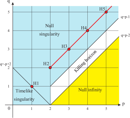
Figure 1: Properties of $r=r_{\rm h}$. This figure should be compared with Fig. 1 in [21].

Now we assume $q>p-2$. Then, $r^{\prime\prime}$ blows up as $r\to r_{\rm h}$ for $2/(q-p+2)<2$ with $2/(q-p+2)\neq 1$, which are identical to $q>p-1$ with $q\neq p$. On the other hand, $H^{\prime\prime}$ blows up as $r\to r_{\rm h}$ for $2q/(q-p+2)<2$ and $2q/(q-p+2)\neq 1$, which are identical to $p<2$ with $q\neq-p+2$. For those parameter regions, $r=r_{\rm h}$ is a curvature singularity by Lemma 3, which is a light blue region in Fig. 1 except for a red point $q=p=1$ and a red line $q=p(\geq 2)$ without including the boundaries given by $q=p-1$ with $p\geq 2$ and $p=2$ with $q\leq 1$. By Lemma 1, the singularity at $r=r_{\rm h}$ is non-null for $q<-p+2$ and null otherwise.

Because both $r^{\prime\prime}$ and $H^{\prime\prime}$ are finite, $r=r_{\rm h}$ is a Killing horizon in the parameter region given by $p-2<q\leq p-1$ and $p\geq 2$, which is a white region in Fig. 1. In contrast, the parameter regions $q=p=1$ and $q=p(\geq 2)$ are more subtle. In such cases, it is necessary to consider the next leading-order terms to check if $r=r_{\rm h}$ is singular or not. In Sec. IV in [21], the authors mentioned a $C^{2}$ extension at $r=r_{\rm h}$ in such a case without taking into account the contribution of higher-order terms. For $q=p=N$, we have

$$\lim_{x\to x_{\rm h}}r(x)\simeq r_{\rm h}+\frac{1}{\sqrt{\gamma_{0}\alpha_{0}}}(x-x_{\rm h})+r_{2}(x-x_{\rm h})^{1+\delta},$$ (A.7)

$$\lim_{x\to x_{\rm h}}H(x)\simeq\gamma_{0}\biggl{(}\frac{1}{\sqrt{\gamma_{0}\alpha_{0}}}\biggl{)}^{N}(x-x_{\rm h})^{N}+H_{2}(x-x_{\rm h})^{N+\eta},$$ (A.8)

where we have included higher-order terms with non-zero constants $r_{2}$ and $H_{2}$ and positive constants $\delta$ and $\eta$. The first and sixth columns in Table I in [21] state that $r=r_{\rm h}$ is regular for $N\in{\mathbb{N}}$, corresponding to the points ${\rm H}1,{\rm H}2,\cdots$ in Fig. 1, and singular otherwise. However, this claim is not correct in general. The correct statement is that $r=r_{\rm h}$ is regular and $C^{2}$ extendible for (i) $N=1$ with $\delta\geq 1$ and $\eta\geq 1$ or (ii) $N\geq 2$ with $\delta\geq 1$, and singular otherwise.

Appendix B Solutions obeying $p_{\rm r}=\chi_{\rm r}\rho$ and $p_{2}=\chi_{\rm t}\rho$ with $\chi_{\rm r}=-1,0$

In this appendix, we study solutions to the Einstein equations for the metric (2.1) with a matter field (3.5) obeying linear relations $p_{\rm r}=\chi_{\rm r}\rho$ and $p_{2}=\chi_{\rm t}\rho$. Then, Eqs. (3.8)–(3.11) are written as

$$(n-2)r^{\prime\prime}H= -\kappa_{n}(1+\chi_{\rm r})\rho r,$$ (B.1)

$$2\kappa_{n}\chi_{\rm r}\rho r^{2}= (n-2)\left[rH^{\prime}r^{\prime}-(n-3)(k-H{r^{\prime}}^{2})\right]+2\Lambda r^{2},$$ (B.2)

$$2\kappa_{n}\chi_{\rm t}\rho r^{2}= r^{2}H^{\prime\prime}+2(n-3)r(H^{\prime}r^{\prime}+Hr^{\prime\prime})-(n-3)(n-4)(k-H{r^{\prime}}^{2})+2\Lambda r^{2}.$$ (B.3)

The conservation equation (3.12) is integrated to give

$$\rho=\rho_{0}r^{-(n-2)(\chi_{\rm r}-\chi_{\rm t})/\chi_{\rm r}}H^{1+\beta},$$ (B.4)

$$\beta:=-\frac{1+3\chi_{\rm r}}{2\chi_{\rm r}}$$ (B.5)

for $\chi_{\rm r}\neq 0$ and

$$H=H_{0}r^{2(n-2)\chi_{\rm t}}$$ (B.6)

for $\chi_{\rm r}=0$, where $\rho_{0}$ and $H_{0}$ are integration constants. Therefore, the case with $\chi_{\rm r}=0$ must be treated separately. This class of solutions with $\chi_{\rm r}=0$ has been obtained in [47] in general relativity and pure Lovelock gravity.

Solution for $\chi_{\rm r}=-1$

We present the most general static solution obeying $p_{\rm r}=-\rho$ and $p_{2}=\chi_{\rm t}\rho$, which generalizes the result in [48] for $n=4$, $k=1$, and $\Lambda=0$. In the case of $\chi_{\rm r}=-1$, Eq. (B.4) reduces to

$$\rho=\rho_{0}r^{-(n-2)(1+\chi_{\rm t})}$$ (B.7)

and Eq. (B.1) gives $r(x)=r_{0}+r_{1}x$, where $r_{0}$ and $r_{1}$ are integration constant. The solution is classified into two subclasses depending on whether $r_{1}$ is zero or not.

In the case of $r_{1}\neq 0$, we can set $r=x$ without loss of generality by a coordinate transformation $r_{0}+r_{1}x\to x$. Then, the general solution is given by

$$H(x)=k-\frac{2M}{x^{n-3}}+\frac{\eta}{x^{(n-2)\chi_{\rm t}+(n-4)}}-\frac{2\Lambda}{(n-1)(n-2)}x^{2},$$ (B.8)

$$r(x)=x,\qquad\rho=\frac{(n-2)[(n-2)\chi_{\rm t}-1]\eta}{2\kappa_{n}x^{(n-2)(1+\chi_{\rm t})}}$$ (B.9)

where $M$ and $\eta$ are constants. In the case of $r_{1}=0$, the general solution is the following direct-product solution

$$H(x)=H_{0}+H_{1}x+H_{2}x^{2},$$ (B.10)

$$r(x)=r_{0},\qquad\rho=\frac{(n-2)(n-3)k-2\Lambda r_{0}^{2}}{2\kappa_{n}r_{0}^{2}},$$ (B.11)

where $r_{0}$, $H_{0}$, and $H_{1}$ are arbitrary constants and $H_{2}$ is given by

$$H_{2}=\frac{k(n-3)[(n-2)\chi_{\rm t}+(n-4)]-2(\chi_{\rm t}+1)\Lambda r_{0}^{2}}{2r_{0}^{2}}.$$ (B.12)

Solution for $\chi_{\rm r}=0$

In the case of $\chi_{\rm r}=0$, substituting Eq. (B.6) into Eq. (B.2), we obtain the master equation for $r(x)$:

$$0=(n-2)[2(n-2)\chi_{\rm t}+(n-3)]H_{0}r^{2(n-2)\chi_{\rm t}}{r^{\prime}}^{2}+2\Lambda r^{2}-k(n-2)(n-3).$$ (B.13)

For $\chi_{\rm t}=-(n-3)/[2(n-2)]$, Eq. (B.13) shows that $r$ is a constant given by

$$r=r_{0}:=\sqrt{\frac{k(n-2)(n-3)}{2\Lambda}},$$ (B.14)

which is real only for $k\Lambda>0$, and hence $H$ is also constant by Eq. (B.6). Then, Eq. (3.8) gives $\rho\equiv 0$ and hence $p_{2}\equiv 0$. Therefore, there is no non-vacuum solution for $\chi_{\rm t}=-(n-3)/[2(n-2)]$ and the only possible solution is the following Nariai-type direct-product vacuum solution;

$$H(x)=H_{0}+H_{1}x-\frac{2\Lambda}{n-2}x^{2},\qquad r(x)=r_{0},$$ (B.15)

where $H_{0}$ and $H_{1}$ are arbitrary constants and $r_{0}$ is given by Eq. (B.14).

For $\chi_{\rm t}\neq-(n-3)/[2(n-2)]$, the master equation (B.13) is integrated to give

$$\pm(x-x_{0})=\int\frac{{\rm d}r}{\sqrt{V(r)}},$$ (B.16)

$$V(r):=\frac{k(n-2)(n-3)-2\Lambda r^{2}}{(n-2)[2(n-2)\chi_{\rm t}+(n-3)]H_{0}r^{2(n-2)\chi_{\rm t}}}.$$ (B.17)

where $x_{0}$ is an integration constant. The solution is real in domains where $V(r)>0$ holds and the energy density is given by

$$\rho= \frac{p_{2}}{\chi_{\rm t}}=\frac{k\chi_{\rm t}(n-3)(n-2)^{2}-2\Lambda[(n-2)\chi_{\rm t}-1]r^{2}}{\kappa_{n}[2(n-2)\chi_{\rm t}+(n-3)]r^{2}}.$$ (B.18)

In the dust case $\chi_{\rm t}=0$, the energy density (B.18) becomes constant such that

$$\rho= \frac{2\Lambda}{(n-3)\kappa_{n}},$$ (B.19)

which shows that there is no non-vacuum solution with $\Lambda=0$ in the dust case.

For $\Lambda=0$, the energy density (B.18) is given by

$$\rho= \frac{p_{2}}{\chi_{\rm t}}=\frac{k\chi_{\rm t}(n-3)(n-2)^{2}}{\kappa_{n}[2(n-2)\chi_{\rm t}+(n-3)]r^{2}}$$ (B.20)

and the solution of the master equation (B.16) is

$$r(x)= \biggl{(}\frac{k(n-3)[(n-2)\chi_{\rm t}+1]^{2}}{[2(n-2)\chi_{\rm t}+(n-3)]H_{0}}\biggl{)}^{1/[2\{(n-2)\chi_{\rm t}+1\}]}(x-x_{0})^{1/[(n-2)\chi_{\rm t}+1]}$$ (B.21)

for $\chi_{\rm t}\neq-1/(n-2)$ and

$$r(x)=\exp\biggl{(}\pm\sqrt{\frac{k(n-3)}{(n-5)H_{0}}}(x-x_{0})\biggl{)}$$ (B.22)

for $\chi_{\rm t}=-1/(n-2)$.

Appendix C Coefficients of $H(x)$ in the asymptotic solutions near a Killing horizon

In this appendix, we explain how to determine the coefficients of $H$ in the asymptotic solutions in Proposition 5. We write Eqs. (3.32)–(3.35) as

$$Hr^{\prime\prime}=-\frac{\kappa_{n}(p_{\rm r}+\rho)r}{n-2},$$ (C.1)

$$H^{\prime}rr^{\prime}=(n-3)k-(n-3)H{r^{\prime}}^{2}+\frac{2(\kappa_{n}p_{\rm r}-\Lambda)r^{2}}{n-2},$$ (C.2)

$$2\kappa_{n}p_{2}r^{2}=H^{\prime\prime}r^{2}+2(n-3)r(H^{\prime}r^{\prime}+Hr^{\prime\prime})-(n-3)(n-4)(k-H{r^{\prime}}^{2})+2\Lambda r^{2}$$ (C.3)

and obtain power series solutions to Eqs. (C.1)–(C.3) up to the order of $|\Delta|^{1+\beta}$.

For $\chi_{\rm r}=-1/(1+2N)$ with $N\in\mathbb{N}$

First we consider the case of $\beta\in\mathbb{N}_{0}(=0,1,2,\cdots)$, which is equivalent to $\chi_{\rm r}=-1/(1+2N)$ with $N\in\mathbb{N}(=1,2,\cdots)$. In this case, substituting the expansions

$$\lim_{x\to x_{\rm h}}H(x)\simeq\sum_{i=1}^{3+\beta}H_{i}\Delta^{i},$$ (C.4)

$$\lim_{x\to x_{\rm h}}r(x)\simeq r_{0}+r_{1}\Delta+r_{2+\beta}\Delta^{2+\beta},$$ (C.5)

$$\lim_{x\to x_{\rm h}}\rho\simeq C_{\rho}\Delta^{1+\beta}$$ (C.6)

into Eq. (C.1), we obtain

$$C_{\rho}=-\frac{(n-2)(2+\beta)(1+\beta)H_{1}r_{2+\beta}}{\kappa_{n}(1+\chi_{\rm r})r_{0}}.$$ (C.7)

Then, substituting Eqs. (C.4)–(C.7) into Eq. (C.2), we obtain

$$r_{0}r_{1}\sum_{i=0}^{1+\beta}(i+1)H_{i+1}\Delta^{i}\simeq(n-3)k-r_{1}^{2}\sum_{i=1}^{1+\beta}(n-3+i)H_{i}\Delta^{i}-\frac{2\Lambda}{n-2}(r_{0}+r_{1}\Delta)^{2}$$ (C.8)

up to the order of $\Delta^{1+\beta}$.

In the case where at least $(n-3)k$ or $\Lambda$ is non-zero, Eq. (C.8) determines the coefficients in $H$ as

$$H_{1}=\frac{(n-2)(n-3)k-2\Lambda{r_{0}}^{2}}{(n-2)r_{0}r_{1}},$$ (C.9)

$$H_{2}=\frac{-(n-2)^{2}(n-3)k+2(n-4)\Lambda{r_{0}}^{2}}{2(n-2){r_{0}}^{2}},$$ (C.10)

$$H_{3}=\frac{(n-3)r_{1}\{(n-1)(n-2)k-2\Lambda{r_{0}}^{2}\}}{6{r_{0}}^{3}}\quad(\mbox{for}~{}\beta\geq 1),$$ (C.11)

$$H_{i+1}=-\frac{(n-3+i)r_{1}}{(1+i)r_{0}}H_{i}\quad(\mbox{with}~{}3\leq i\leq 1+\beta~{}\mbox{for}~{}\beta\geq 2),$$ (C.12)

while $H_{3+\beta}$ is undetermined. Then, substituting those results into Eq. (C.3), we obtain

$$2\kappa_{n}\chi_{\rm t}{r_{0}}^{2}C_{\rho}\Delta^{1+\beta}-2(n-3)(2+\beta)^{2}H_{1}r_{0}r_{2+\beta}\Delta^{1+\beta}$$

$$\simeq{r_{0}}^{2}\sum_{i=0}^{1+\beta}(i+2)(i+1)H_{i+2}\Delta^{i}+2r_{0}r_{1}\sum_{i=0}^{1+\beta}(n-3+i)(i+1)H_{i+1}\Delta^{i}$$

$$+{r_{1}}^{2}\sum_{i=1}^{1+\beta}\{(n-3)(n-4+2i)+i(i-1)\}H_{i}\Delta^{i}-(n-3)(n-4)k+2\Lambda(r_{0}+r_{1}\Delta)^{2}.$$ (C.13)

We note that $\Delta^{2}$ terms contribute only if $\beta\geq 1$ and the terms with $\sum_{i=3}^{1+\beta}$ contribute only if $\beta\geq 2$. For $\beta=0$, the terms of the order $\Delta^{0}$ are canceled by Eqs. (C.9) and (C.10) and the terms of the order $\Delta^{1}$ give

$$H_{3}= \frac{(n-3)r_{1}\left\{(n-1)(n-2)k-2\Lambda{r_{0}}^{2}\right\}}{6{r_{0}}^{3}}-\frac{2H_{1}r_{2}}{3r_{0}}\biggl{\{}\frac{(n-2)\chi_{\rm t}}{1+\chi_{\rm r}}+2(n-3)\biggl{\}}.$$ (C.14)

For $\beta=1$, the terms of the order $\Delta^{0}$ are canceled by Eqs. (C.9) and (C.10), the terms of the order $\Delta^{1}$ are canceled by Eqs. (C.9)–(C.11), and the terms of the order $\Delta^{2}$ give

$$H_{4}= -\frac{n(n-3){r_{1}}^{2}\left\{(n-1)(n-2)k-2\Lambda{r_{0}}^{2}\right\}}{24{r_{0}}^{4}}-\frac{H_{1}r_{3}}{2r_{0}}\biggl{\{}\frac{2(n-2)\chi_{\rm t}}{1+\chi_{\rm r}}+3(n-3)\biggl{\}}.$$ (C.15)

For $\beta\geq 2$, using Eqs. (C.9)–(C.11), we write Eq. (C.13) as

$$2\kappa_{n}\chi_{\rm t}{r_{0}}^{2}C_{\rho}\Delta^{1+\beta}-2(n-3)(2+\beta)^{2}H_{1}r_{0}r_{2+\beta}\Delta^{1+\beta}$$

$$\simeq{r_{0}}^{2}\sum_{i=3}^{\beta}(i+2)(i+1)H_{i+2}\Delta^{i}+{r_{0}}^{2}(3+\beta)(2+\beta)H_{3+\beta}\Delta^{1+\beta}$$

$$~{}~{}~{}+2r_{0}r_{1}\sum_{i=3}^{\beta}(n-3+i)(i+1)H_{i+1}\Delta^{i}+2r_{0}r_{1}(n-2+\beta)(2+\beta)H_{2+\beta}\Delta^{1+\beta}$$

$$~{}~{}~{}+{r_{1}}^{2}\sum_{i=3}^{\beta}\{(n-3)(n-4+2i)+i(i-1)\}H_{i}\Delta^{i}$$

$$~{}~{}~{}+{r_{1}}^{2}\{(n-3)(n-2+2\beta)+\beta(1+\beta)\}H_{1+\beta}\Delta^{1+\beta}.$$ (C.16)

Since the terms with $\sum_{i=3}^{\beta}$ are canceled by Eq. (C.12), we obtain

$$H_{3+\beta}= \frac{{r_{1}}^{2}(n-1+\beta)(n-2+\beta)}{{r_{0}}^{2}(3+\beta)(2+\beta)}H_{1+\beta}$$

$$-\frac{2H_{1}r_{2+\beta}}{(3+\beta)r_{0}}\biggl{\{}\frac{(1+\beta)(n-2)\chi_{\rm t}}{1+\chi_{\rm r}}+(2+\beta)(n-3)\biggl{\}},$$ (C.17)

where $H_{1+\beta}$ on the right-hand side can be written in terms of $r_{0}$ and $r_{1}$ by Eqs. (C.11) and (C.12). In this case, the parameters are $r_{0}$, $r_{1}$, and $r_{2+\beta}$.

For $(n-3)k=\Lambda=0$, Eq. (C.8) is satisfied for $r_{1}=0$. Then, substituting the results into Eq. (C.3), we obtain

$$2\kappa_{n}\chi_{\rm t}r_{0}^{2}C_{\rho}\Delta^{1+\beta}\simeq {r_{0}}^{2}\sum_{i=0}^{1+\beta}(i+2)(i+1)H_{i+2}\Delta^{i}+2(n-3)(2+\beta)^{2}r_{0}r_{2+\beta}H_{1}\Delta^{1+\beta}$$ (C.18)

up to the order of $\Delta^{1+\beta}$, which shows that

$$\begin{aligned} &H_{2}=H_{3}=\cdots=H_{1+\beta}=H_{2+\beta}=0,\\ &H_{3+\beta}=-\frac{2H_{1}r_{2+\beta}}{(3+\beta)r_{0}}\biggl{\{}(n-3)(2+\beta)+\frac{\chi_{\rm t}(n-2)(1+\beta)}{1+\chi_{\rm r}}\biggl{\}}.\end{aligned}$$ (C.19)

In this case, the parameters are $r_{0}$, $r_{2+\beta}$, and $H_{1}$.

For $\chi_{\rm r}\neq-1/(1+2N)$ with $N\in\mathbb{N}$

Next we consider a non-integer positive $\beta$, which is equivalent to $\chi_{\rm r}\neq-1/(1+2N)$ with $N\in\mathbb{N}(=1,2,\cdots)$. In this case, we study the domains $x\geq x_{\rm h}$ and $x\leq x_{\rm h}$ separately.

In the domain $x\geq x_{\rm h}$, substituting the expansions

$$\lim_{x\to x_{\rm h}}H(x)\simeq\sum_{i=1}^{[3+\beta]}H_{i}\Delta^{i}+H_{2+\beta}\Delta^{2+\beta}+H_{3+\beta}\Delta^{3+\beta},$$ (C.20)

$$\lim_{x\to x_{\rm h}}r(x)\simeq r_{0}+r_{1}\Delta+r_{2+\beta}\Delta^{2+\beta},$$ (C.21)

$$\lim_{x\to x_{\rm h}}\rho\simeq C_{\rho}\Delta^{1+\beta}$$ (C.22)

into Eq. (C.1), we obtain Eq. (C.7). Then, substituting the results into Eq. (C.2), we obtain

$$r_{0}r_{1}\sum_{i=0}^{[1+\beta]}(i+1)H_{i+1}\Delta^{i}+(2+\beta)r_{0}r_{1}H_{2+\beta}\Delta^{1+\beta}$$

$$\simeq (n-3)k-r_{1}^{2}\sum_{i=1}^{[1+\beta]}(n-3+i)H_{i}\Delta^{i}-\frac{2\Lambda}{n-2}(r_{0}^{2}+2r_{0}r_{1}\Delta+{r_{1}}^{2}\Delta^{2})$$ (C.23)

up to the order of $\Delta^{1+\beta}$.

In the case where at least $(n-3)k$ or $\Lambda$ is non-zero, Eq. (C.23) determines the coefficients in $H$ as

$$H_{1}=\frac{(n-2)(n-3)k-2\Lambda{r_{0}}^{2}}{(n-2)r_{0}r_{1}},$$ (C.24)

$$H_{2}=\frac{-(n-2)^{2}(n-3)k+2(n-4)\Lambda{r_{0}}^{2}}{2(n-2){r_{0}}^{2}},$$ (C.25)

$$H_{3}=\frac{(n-3)r_{1}\{(n-1)(n-2)k-2\Lambda{r_{0}}^{2}\}}{6{r_{0}}^{3}}\quad(\mbox{for}~{}\beta>1),$$ (C.26)

$$H_{i+1}=-\frac{(n-3+i)r_{1}}{(1+i)r_{0}}H_{i}\quad(\mbox{for}~{}3\leq i\leq[1+\beta]~{}\mbox{if}~{}\beta>2),$$ (C.27)

$$H_{2+\beta}=0,$$ (C.28)

while $H_{[3+\beta]}$ and $H_{3+\beta}$ are undetermined.

Then, substituting those results into Eq. (C.3), we obtain

$$2\kappa_{n}\chi_{\rm t}{r_{0}}^{2}C_{\rho}\Delta^{1+\beta}-2(n-3)(2+\beta)^{2}H_{1}r_{0}r_{2+\beta}\Delta^{1+\beta}-(3+\beta)(2+\beta){r_{0}}^{2}H_{3+\beta}\Delta^{1+\beta}$$

$$\simeq 6{r_{0}}^{2}H_{3}\Delta+4(n-2)r_{0}r_{1}H_{2}\Delta+(n-3)(n-2){r_{1}}^{2}H_{1}\Delta+4\Lambda r_{0}r_{1}\Delta$$

$$~{}~{}~{}+12{r_{0}}^{2}H_{4}\Delta^{2}+6(n-1)r_{0}r_{1}H_{3}\Delta^{2}+(n-1)(n-2){r_{1}}^{2}H_{2}\Delta^{2}+2\Lambda{r_{1}}^{2}\Delta^{2}$$

$$~{}~{}~{}+{r_{0}}^{2}\sum_{i=3}^{[1+\beta]}(i+2)(i+1)H_{i+2}\Delta^{i}+2r_{0}r_{1}\sum_{i=3}^{[1+\beta]}(n-3+i)(i+1)H_{i+1}\Delta^{i}$$

$$~{}~{}~{}+{r_{1}}^{2}\sum_{i=3}^{[1+\beta]}\{(n-3)(n-4+2i)+i(i-1)\}H_{i}\Delta^{i}$$ (C.29)

up to the order of $\Delta^{1+\beta}$. We note that $\Delta^{2}$ terms contribute only if $\beta>1$ and the terms with $\sum_{i=3}^{[1+\beta]}$ contribute only if $\beta>2$. From the terms of the order $\Delta^{1+\beta}$, we obtain

$$H_{3+\beta}= -\frac{2H_{1}r_{2+\beta}}{(3+\beta)r_{0}}\biggl{\{}(n-3)(2+\beta)+\frac{(n-2)(1+\beta)\chi_{\rm t}}{1+\chi_{\rm r}}\biggl{\}}.$$ (C.30)

The expression of $H_{[3+\beta]}$ is obtained as follows. For $0<\beta<1$, the terms of the order $\Delta^{1}$ with Eqs. (C.24) and (C.25) give

$$H_{3}(=H_{[3+\beta]})=\frac{(n-3)r_{1}\{(n-1)(n-2)k-2\Lambda{r_{0}}^{2}\}}{6{r_{0}}^{3}}\quad(\mbox{for}~{}0<\beta<1).$$ (C.31)

Then, for $1<\beta<2$, the terms of the order $\Delta^{2}$ with Eqs. (C.24)–(C.26) give

$$H_{4}(=H_{[3+\beta]})= -\frac{n(n-3){r_{1}}^{2}\{(n-1)(n-2)k-2\Lambda{r_{0}}^{2}\}}{24{r_{0}}^{4}}$$

$$= -\frac{nr_{1}}{4r_{0}}H_{3}\quad(\mbox{for}~{}1<\beta<2).$$ (C.32)

For $\beta>2$, the terms of the order $\Delta^{[1+\beta]}$ give

$$H_{[3+\beta]}= -\frac{2r_{1}[n-2+\beta]}{r_{0}[3+\beta]}H_{[2+\beta]}$$

$$-\frac{{r_{1}}^{2}\{(n-3)(n-4+2[1+\beta])+[1+\beta][\beta]\}}{{r_{0}}^{2}[3+\beta][2+\beta]}H_{[1+\beta]}.$$ (C.33)

In this case, the parameters are $r_{0}$, $r_{1}$, and $r_{2+\beta}$.

For $(n-3)k=\Lambda=0$, Eq. (C.23) is satisfied for $r_{1}=0$. Then, substituting those results into Eq. (C.3), we obtain

$$2\kappa_{n}\chi_{\rm t}r_{0}^{2}C_{\rho}\Delta^{1+\beta}\simeq {r_{0}}^{2}\sum_{i=0}^{[1+\beta]}(i+2)(i+1)H_{i+2}\Delta^{i}+(2+\beta)(1+\beta){r_{0}}^{2}H_{2+\beta}\Delta^{\beta}$$

$$+(3+\beta)(2+\beta){r_{0}}^{2}H_{3+\beta}\Delta^{1+\beta}+2(n-3)(2+\beta)^{2}r_{0}r_{2+\beta}H_{1}\Delta^{1+\beta}$$ (C.34)

up to the order of $\Delta^{1+\beta}$, which shows

$$H_{2}=H_{3}=\cdots=H_{[2+\beta]}=H_{[3+\beta]}=0,\qquad H_{2+\beta}=0$$ (C.35)

and $H_{3+\beta}$ given by Eq. (C.19). In this case, the parameters are $r_{0}$, $r_{2+\beta}$, and $H_{1}$.

In the domain $x\leq x_{\rm h}$, substituting the expansions

$$\lim_{x\to x_{\rm h}}H(x)\simeq\sum_{i=1}^{[3+\beta]}H_{i}\Delta^{i}+{\bar{H}}_{2+\beta}(-\Delta)^{2+\beta}+{\bar{H}}_{3+\beta}(-\Delta)^{3+\beta},$$ (C.36)

$$\lim_{x\to x_{\rm h}}r(x)\simeq r_{0}+r_{1}\Delta+{\bar{r}}_{2+\beta}(-\Delta)^{2+\beta},$$ (C.37)

$$\lim_{x\to x_{\rm h}}\rho\simeq{\bar{C}}_{\rho}(-\Delta)^{1+\beta}.$$ (C.38)

into Eq. (C.1), we obtain

$${\bar{C}}_{\rho}=\frac{(n-2)(2+\beta)(1+\beta)H_{1}{\bar{r}}_{2+\beta}}{\kappa_{n}(1+\chi_{\rm r})r_{0}}.$$ (C.39)

Then, substituting Eqs. (C.36)–(C.39) into Eq. (C.2), we obtain

$$r_{0}r_{1}\sum_{i=0}^{[1+\beta]}(i+1)H_{i+1}\Delta^{i}-(2+\beta)r_{0}r_{1}{\bar{H}}_{2+\beta}(-\Delta)^{1+\beta}$$

$$\simeq (n-3)k-{r_{1}}^{2}\sum_{i=1}^{[1+\beta]}(n-3+i)H_{i}\Delta^{i}-\frac{2\Lambda}{n-2}({r_{0}}^{2}+2r_{0}r_{1}\Delta+{r_{1}}^{2}\Delta^{2})$$ (C.40)

up to the order of $(-\Delta)^{1+\beta}$.

In the case where at least $(n-3)k$ or $\Lambda$ is non-zero, Eq. (C.40) determines the coefficients in $H$ as Eqs. (C.24)–(C.27) and ${\bar{H}}_{2+\beta}=0$. Then, substituting those results into Eq. (C.3), we obtain

$$2\kappa_{n}\chi_{\rm t}{r_{0}}^{2}{\bar{C}}_{\rho}(-\Delta)^{1+\beta}$$

$$+2(n-3)(2+\beta)^{2}H_{1}r_{0}{\bar{r}}_{2+\beta}(-\Delta)^{1+\beta}-(3+\beta)(2+\beta){r_{0}}^{2}{\bar{H}}_{3+\beta}(-\Delta)^{1+\beta}$$

$$\simeq 6{r_{0}}^{2}H_{3}\Delta+4(n-2)r_{0}r_{1}H_{2}\Delta+(n-3)(n-2){r_{1}}^{2}H_{1}\Delta+4\Lambda r_{0}r_{1}\Delta$$

$$~{}~{}~{}+12{r_{0}}^{2}H_{4}\Delta^{2}+6(n-1)r_{0}r_{1}H_{3}\Delta^{2}+(n-1)(n-2){r_{1}}^{2}H_{2}\Delta^{2}+2\Lambda{r_{1}}^{2}\Delta^{2}$$

$$~{}~{}~{}+{r_{0}}^{2}\sum_{i=3}^{[1+\beta]}(i+2)(i+1)H_{i+2}\Delta^{i}+2r_{0}r_{1}\sum_{i=3}^{[1+\beta]}(n-3+i)(i+1)H_{i+1}\Delta^{i}$$

$$~{}~{}~{}+{r_{1}}^{2}\sum_{i=3}^{[1+\beta]}\{(n-3)(n-4+2i)+i(i-1)\}H_{i}\Delta^{i}$$ (C.41)

up to the order of $(-\Delta)^{1+\beta}$. From the terms of the order $\Delta^{1+\beta}$, we obtain

$${\bar{H}}_{3+\beta}= \frac{2H_{1}{\bar{r}}_{2+\beta}}{(3+\beta)r_{0}}\biggl{\{}(n-3)(2+\beta)+\frac{(n-2)(1+\beta)\chi_{\rm t}}{1+\chi_{\rm r}}\biggl{\}}.$$ (C.42)

Since the right-hand sides of Eqs. (C.29) and (C.41) are identical, Eqs. (C.31)–(C.33) are valid as the expressions of $H_{[3+\beta]}$ for $0<\beta<1$, for $1<\beta<2$, and for $\beta>2$, respectively. In this case, the parameters are $r_{0}$, $r_{1}$, and ${\bar{r}}_{2+\beta}$.

For $(n-3)k=\Lambda=0$, Eq. (C.40) is satisfied for $r_{1}=0$. Then, substituting those results into Eq. (C.3), we obtain

$$2\kappa_{n}\chi_{\rm t}{r_{0}}^{2}{\bar{C}}_{\rho}(-\Delta)^{1+\beta}\simeq {r_{0}}^{2}\sum_{i=0}^{[1+\beta]}(i+2)(i+1)H_{i+2}\Delta^{i}+(2+\beta)(1+\beta){r_{0}}^{2}{\bar{H}}_{2+\beta}(-\Delta)^{\beta}$$

$$+(3+\beta)(2+\beta){r_{0}}^{2}{\bar{H}}_{3+\beta}(-\Delta)^{1+\beta}$$

$$-2(n-3)(2+\beta)^{2}r_{0}{\bar{r}}_{2+\beta}H_{1}(-\Delta)^{1+\beta}$$ (C.43)

up to the order of $(-\Delta)^{1+\beta}$. For $\beta\notin\mathbb{N}$, the above equation shows

$$H_{2}=H_{3}=\cdots=H_{[2+\beta]}=H_{[3+\beta]}=0,\qquad{\bar{H}}_{2+\beta}=0$$ (C.44)

and ${\bar{H}}_{3+\beta}$ given by Eq. (C.42). In this case, the parameters are $r_{0}$, ${\bar{r}}_{2+\beta}$, and $H_{1}$.

References

- [1] S. W. Hawking, “Black holes in general relativity,” Commun. Math. Phys. 25, 152 (1972) doi:10.1007/BF01877517
- [2] S. W. Hawking and G. F. R. Ellis, The large scale structure of space-time, (Cambridge University Press, Cambridge, 1973).
- [3] P. T. Chruściel, “On rigidity of analytic black holes,” Commun. Math. Phys. 189, 1(1997) doi:10.1007/s002200050187 [arXiv:gr-qc/9610011 [gr-qc]].
- [4] S. Hollands, A. Ishibashi and R. M. Wald, “A higher dimensional stationary rotating black hole must be axisymmetric,” Commun. Math. Phys. 271, 699 (2007) doi:10.1007/s00220-007-0216-4 [arXiv:gr-qc/0605106 [gr-qc]].
- [5] J. M. Bardeen, B. Carter and S. W. Hawking, “The four laws of black hole mechanics,” Commun. Math. Phys. 31, 161 (1973) doi:10.1007/BF01645742
- [6] S. W. Hawking, “Particle Creation By Black Holes,” Commun. Math. Phys. 43, 199 (1975) [Erratum-ibid. 46, 206 (1976)] doi:10.1007/BF02345020
- [7] R. M. Wald, Quantum Field Theory in Curved Spacetime and Black Hole Thermodynamics, (University of Chicago Press, 1994).
- [8] R. M. Wald, “Black hole entropy is the Noether charge,” Phys. Rev. D 48, no.8, R3427 (1993) doi:10.1103/PhysRevD.48.R3427 [arXiv:gr-qc/9307038 [gr-qc]].
- [9] V. Iyer and R. M. Wald, “Some properties of Noether charge and a proposal for dynamical black hole entropy,” Phys. Rev. D 50, 846 (1994) doi:10.1103/PhysRevD.50.846 [arXiv:gr-qc/9403028 [gr-qc]].
- [10] V. Iyer and R. M. Wald, “A comparison of Noether charge and Euclidean methods for computing the entropy of stationary black holes,” Phys. Rev. D 52, 4430(1995) doi:10.1103/PhysRevD.52.4430 [arXiv:gr-qc/9503052 [gr-qc]].
- [11] S. D. Majumdar, “A class of exact solutions of Einstein’s field equations,” Phys. Rev. 72 (1947), 390-398 doi:10.1103/PhysRev.72.390
- [12] A. Papapetrou, “A static solution of the equations of the gravitational field for an arbitrary charge distribution,” Proc. Roy. Irish Acad. A 51 (1947), 191-204. http://www.jstor.org/stable/20488481
- [13] J. P. S. Lemos and V. T. Zanchin, “A class of exact solutions of Einstein’s field equations in higher dimensional spacetimes, d = 4: Majumdar-Papapetrou solutions,” Phys. Rev. D 71 (2005), 124021 doi:10.1103/PhysRevD.71.124021 [arXiv:gr-qc/0505142 [gr-qc]].
- [14] J. B. Hartle and S. W. Hawking, “Solutions of the Einstein-Maxwell equations with many black holes,” Commun. Math. Phys. 26 (1972), 87-101 doi:10.1007/BF01645696
- [15] G. N. Candlish and H. S. Reall, “On the smoothness of static multi-black hole solutions of higher-dimensional Einstein-Maxwell theory,” Class. Quant. Grav. 24 (2007), 6025-6040 doi:10.1088/0264-9381/24/23/022 [arXiv:0707.4420 [gr-qc]].
- [16] D. L. Welch, “On the smoothness of the horizons of multi - black hole solutions,” Phys. Rev. D 52 (1995), 985-991 doi:10.1103/PhysRevD.52.985 [arXiv:hep-th/9502146 [hep-th]].
- [17] H. Maeda, “Vacuum-dual static perfect fluid obeying in dimensions,” Class. Quant. Grav. 40 (2023) no.8, 085014 doi:10.1088/1361-6382/acc3f1 [arXiv:2210.10795 [gr-qc]].
- [18] V. Pravda and O. B. Zaslavskii, “Curvature tensors on distorted Killing horizons and their algebraic classification,” Class. Quant. Grav. 22 (2005), 5053-5072 doi:10.1088/0264-9381/22/23/009 [arXiv:gr-qc/0510095 [gr-qc]].
- [19] O. B. Zaslavskii, “Truly naked spherically-symmetric and distorted black holes,” Phys. Rev. D 76 (2007), 024015 doi:10.1103/PhysRevD.76.024015 [arXiv:0706.2727 [gr-qc]].
- [20] K. A. Bronnikov and O. B. Zaslavskii, “Black holes can have curly hair,” Phys. Rev. D 78 (2008), 021501 doi:10.1103/PhysRevD.78.021501 [arXiv:0801.0889 [gr-qc]].
- [21] K. A. Bronnikov, E. Elizalde, S. D. Odintsov and O. B. Zaslavskii, “Horizons vs. singularities in spherically symmetric space-times,” Phys. Rev. D 78 (2008), 064049 doi:10.1103/PhysRevD.78.064049 [arXiv:0805.1095 [gr-qc]].
- [22] K. A. Bronnikov and O. B. Zaslavskii, “General static black holes in matter,” Class. Quant. Grav. 26 (2009), 165004 doi:10.1088/0264-9381/26/16/165004 [arXiv:0904.4904 [gr-qc]].
- [23] K. A. Bronnikov and O. B. Zaslavskii, “Neutral and charged matter in equilibrium with black holes,” Phys. Rev. D 84 (2011), 084013 doi:10.1103/PhysRevD.84.084013 [arXiv:1107.4701 [gr-qc]].
- [24] M. Visser, “Dirty black holes: Thermodynamics and horizon structure,” Phys. Rev. D 46 (1992), 2445-2451 doi:10.1103/PhysRevD.46.2445 [arXiv:hep-th/9203057 [hep-th]].
- [25] G. T. Horowitz and S. F. Ross, “Naked black holes,” Phys. Rev. D 56 (1997), 2180-2187 doi:10.1103/PhysRevD.56.2180 [arXiv:hep-th/9704058 [hep-th]].
- [26] G. T. Horowitz and S. F. Ross, “Properties of naked black holes,” Phys. Rev. D 57 (1998), 1098-1107 doi:10.1103/PhysRevD.57.1098 [arXiv:hep-th/9709050 [hep-th]].
- [27] D. Lovelock, “The Einstein tensor and its generalizations,” J. Math. Phys. 12 (1971), 498-501 doi:10.1063/1.1665613
- [28] M. J. S. L. Ashley and S. M. Scott, “Curvature singularities and abstract boundary singularity theorems for space-time,” [arXiv:gr-qc/0309070 [gr-qc]].
- [29] R. Steinbauer, “The singularity theorems of General Relativity and their low regularity extensions,” doi:10.1365/s13291-022-00263-7 [arXiv:2206.05939 [math-ph]].
- [30] C. Barrabès and W. Israel, “Thin shells in general relativity and cosmology: The Lightlike limit,” Phys. Rev. D 43, 1129 (1991). doi:10.1103/PhysRevD.43.1129
- [31] E. Poisson, “A Reformulation of the Barrabès-Israel null shell formalism”, gr-qc/0207101.
- [32] E. Poisson, A Relativist’s Toolkit, (Cambridge University Press, 2004).
- [33] L. Avilés, H. Maeda and C. Martínez, “Junction conditions in scalar–tensor theories,” Class. Quant. Grav. 37 (2020) no.7, 075022 doi:10.1088/1361-6382/ab728a [arXiv:1910.07534 [gr-qc]].
- [34] H. Maeda and T. Harada, “Criteria for energy conditions,” Class. Quant. Grav. 39 (2022) no.19, 195002 doi:10.1088/1361-6382/ac8861 [arXiv:2205.12993 [gr-qc]].
- [35] H. Maeda and C. Martínez, “Energy conditions in arbitrary dimensions,” PTEP 2020, no.4, 043E02 (2020). doi:10.1093/ptep/ptaa009 [arXiv:1810.02487 [gr-qc]].
- [36] İ. Semiz, “The general static spherical solution with EoS parameter w = 1/5,” Class. Quant. Grav. 39 (2022) no.21, 215002 doi:10.1088/1361-6382/ac8cca [arXiv:2007.08166 [gr-qc]].
- [37] H. Maeda, “Hawking-Ellis type of matter on Killing horizons in symmetric spacetimes,” Phys. Rev. D 104 (2021) no.8, 8 doi:10.1103/PhysRevD.104.084088 [arXiv:2107.01455 [gr-qc]].
- [38] V. Faraoni and J. Côté, “Scalar field as a null dust,” Eur. Phys. J. C 79 (2019) no.4, 318 doi:10.1140/epjc/s10052-019-6829-x [arXiv:1812.06457 [gr-qc]].
- [39] H. Maeda, S. Willison and S. Ray, “Lovelock black holes with maximally symmetric horizons,” Class. Quant. Grav. 28 (2011), 165005 doi:10.1088/0264-9381/28/16/165005 [arXiv:1103.4184 [gr-qc]].
- [40] G. Dotti and R. J. Gleiser, “Obstructions on the horizon geometry from string theory corrections to Einstein gravity,” Phys. Lett. B 627 (2005), 174-179 doi:10.1016/j.physletb.2005.08.110 [arXiv:hep-th/0508118 [hep-th]].
- [41] H. Maeda, “Gauss-Bonnet black holes with non-constant curvature horizons,” Phys. Rev. D 81 (2010), 124007 doi:10.1103/PhysRevD.81.124007 [arXiv:1004.0917 [gr-qc]].
- [42] S. Ray, “Birkhoff’s theorem in Lovelock gravity for general base manifolds,” Class. Quant. Grav. 32 (2015) no.19, 195022 doi:10.1088/0264-9381/32/19/195022 [arXiv:1505.03830 [gr-qc]].
- [43] S. Ohashi and M. Nozawa, “Lovelock black holes with a nonconstant curvature horizon,” Phys. Rev. D 92 (2015), 064020 doi:10.1103/PhysRevD.92.064020 [arXiv:1507.04496 [gr-qc]].
- [44] H. D. Wahlquist, “Interior Solution for a Finite Rotating Body of Perfect Fluid,” Phys. Rev. 172 (1968), 1291-1296 doi:10.1103/PhysRev.172.1291
- [45] J. M. M. Senovilla “Stationary axisymmetric perfect-fluid metrics with const,” Phys. Lett. A 123 (1987), 211-214 doi.org/10.1016/0375-9601(87)90062-4
- [46] K. Hinoue, T. Houri, C. Rugina and Y. Yasui, “General Wahlquist Metrics in All Dimensions,” Phys. Rev. D 90 (2014) no.2, 024037 doi:10.1103/PhysRevD.90.024037 [arXiv:1402.6904 [gr-qc]].
- [47] S. Biswas and C. Singha, “Looking for static interior solutions of Buchdahl star with in general relativity and pure Lovelock theories,” [arXiv:2305.02768 [gr-qc]].
- [48] I. Cho and H. C. Kim, “Simple black holes with anisotropic fluid,” Chin. Phys. C 43 (2019) no.2, 025101 doi:10.1088/1674-1137/43/2/025101 [arXiv:1703.01103 [gr-qc]].