Fundamental, Harmonic, and Third-harmonic Plasma Emission from Beam-plasma Instabilities: A First-principles Precursor for Astrophysical Radio Bursts
Abstract
Electromagnetic fundamental and harmonic emission is ubiquitously observed throughout the heliosphere, and in particular it is commonly associated with the occurrence of Type II and III solar radio bursts. Classical analytic calculations for the plasma-emission process, though useful, are limited to idealized situations; a conclusive numerical verification of this theory is still lacking, with earlier studies often providing contradicting results on e.g. the precise parameter space in which fundamental and harmonic emission can be produced. To accurately capture the chain of mechanisms underlying plasma emission — from precursor plasma processes to the generation of electromagnetic waves over long times — we perform large-scale, first-principles simulations of beam-plasma instabilities. By employing a very large number of computational particles we achieve very low numerical noise, and explore (with an array of simulations) a wide parameter space determined by the beam-plasma density ratio and the ion-to-electron temperature ratio. In particular, we observe direct evidence of both fundamental and harmonic plasma emission when the beam-to-background density ratio (with beam-to-background energy ratio ), tightly constraining this threshold. We observe that, asymptotically, in this regime of the initial beam energy is converted into harmonic emission, and into fundamental emission. In contrast with previous studies, we also find that this emission is independent of the ion-to-electron temperature ratio. In addition, we report the direct detection of third-harmonic emission in all of our simulations, at power levels compatible with observations. Our findings have important consequences for understanding the viable conditions leading to plasma emission in space systems, and for the interpretation of observed electromagnetic signals throughout the heliosphere.
keywords:
Sun: radio radiation – (transients:) fast radio bursts – waves1 Introduction
The production of electromagnetic waves is frequently observed during energetic outbursts from the solar surface, e.g. as Type II and III radio bursts (e.g. Dulk 1985; Stanislavsky et al. 2022). Such observations allow us to probe the plasma conditions of solar eruptive events (e.g. Wild & Smerd 1972; Reid & Ratcliffe 2014; Ndacyayisenga et al. 2023 and references therein), and commonly report the presence of waves at a frequency equal to and/or double the local electron plasma frequency (where and are the electron charge and mass, and is the local electron density). Despite decades of research, however, it is still rather unclear how exactly such “fundamental” (at ) and “harmonic” (at ) emission originates from collective plasma mechanisms.
Theoretical work on the subject spans several decades and has converged on the widely accepted three-wave-interaction model (Ginzburg & Zhelezniakov 1958; Melrose 1970a, b; Zheleznyakov & Zaitsev 1970; Melrose 2017). The latter considers a two-stage process initiated by the excitation of forward-propagating Langmuir () waves, e.g. via the nonlinear evolution of a precursor electrostatic instability. Fundamental emission can then directly originate from the decay of waves (found along the Langmuir dispersion curve, , with the electron thermal speed) into ion acoustic waves (IAWs) (labeled ) and electromagnetic waves (, found along the plasma dispersion curve , where is the speed of light) at approximately the local . Forward-propagating electrostatic waves can also coalesce with, or decay into, IAWs (labeled , which are distinct from ) to produce backward-propagating () modes; the subsequent interaction results in harmonic electromagnetic emission ( waves). The whole process can be summarized as
| (Fundamental emission) | |||
| (Harmonic emission) |
and this three-wave interaction satisfies conservation of momentum and energy in the weak-turbulence limit (e.g. Tsytovich 1972). Hence, each step of the process directly translates into requency and wavenumber sums.
Despite general agreement on the mechanism originating plasma emission, no direct numerical simulation of the whole process (starting from the initial instability to the nonlinear wave-wave interaction) has provided conclusive results supporting analytic calculations. This is mainly due to the tremendous computational resources involved: fully kinetic simulations are necessary, with large (ion-scale) system sizes evolved for long times (much longer than the instability relaxation time) while fully resolving the electron physics. Additionally, the modes involved are expected to grow and saturate only up to a small fraction of the input kinetic energy, implying that numerical noise must be kept very low. Previous works attempting such simulations have focused on fully kinetic Particle-in-Cell (PIC) methods applied to the interaction of dilute electron beams with a cold plasma background, which ideally initiates the plasma-emission process (e.g. Cairns & Robinson 1998). These simulations are very demanding, and involve specific choices of the ion-to-electron temperature ratio and very low beam-to-background density ratios. The latter results in very long quasilinear relaxation times and large computational costs. A low density ratio is however absolutely necessary: the Langmuir dispersion relation can be severely modified by the beam when the density ratio is (see Cairns 1989), producing unstable modes at frequencies substantially different from the electron plasma frequency . This is detrimental for plasma emission, since these modified waves cannot participate in the process discussed above due to a violation of matching conditions: waves cannot exist at frequencies much larger or smaller than the corresponding IAW frequency , and therefore they cannot compensate for the smaller or larger obtained in this case. Low density ratios are therefore essential to maintain the coupling between beam and Langmuir unstable modes at (approximately) , resulting in electrostatic fluctuations that can initiate the three-wave interaction.
In simulations, harmonic emission has been reportedly observed in one- and two-dimensional setups with a single electron beam, multiple counterstreaming beams, and with and without background magnetic fields (e.g. Kasaba et al. 2001; Sakai et al. 2005; Umeda 2010; Tsiklauri 2011; Thurgood & Tsiklauri 2015, 2016; Henri et al. 2019; Lee et al. 2019; Krafft & Savoini 2022a; Lee et al. 2022; Lazar et al. 2023). Thurgood & Tsiklauri (2015) provided a first decisive demonstration of plasma emission in numerical calculations. That work showed that the possibility of plasma emission is contingent upon the frequency of the initial electrostatic waves generated by the beam-plasma instability, and that these waves may be prohibited from participating in the necessary three-wave interactions due to frequency conservation requirements. However, strong evidence for clearly distinguishable fundamental emission (expected to arise with much smaller power than the harmonic signal) was not ubiquitously detected. In addition, the precise plasma conditions (particularly the threshold beam-to-background density ratio and ion-to-electron temperature ratio) under which harmonic emission occurs have yet to be conclusively identified in simulations. In essence, a thorough quantification of the saturated energy level of different modes and of the parameter space in which the three-wave interaction occurs is still missing. This information is however not only fundamental to understand the origin of commonly observed radio signals in space, but also for experiments attempting to reproduce space-plasma conditions (e.g. Marquès et al. 2020 and references therein). We also note that, during the development of this work, a first conclusive detection of fundamental modes in PIC simulations of beam-plasma systems was reported by Zhang et al. (2022), providing numerical evidence to support the three-wave-interaction model of plasma emission.
In this Letter we build on past groundwork by performing an array of PIC simulations of beam-plasma interaction, with the aim to observe and quantify the subsequent plasma emission and the saturated energy levels of each mode involved in the process. Our multidimensional simulations are of very large size111Only surpassed in domain size by the slightly larger run presented in Krafft & Savoini (2022a). and unprecedented duration, to accurately capture the nonlinear evolution of the system over long time scales and to comfortably fit all the wave modes involved in the mechanisms of interest; to obtain converged and reliable results, in our runs we achieve very low levels of numerical noise by employing large numbers of particles per cell. With this approach, we explore the dependence of plasma emission on the initial plasma conditions by varying the beam-to-background density ratio and the ion-to-electron temperature ratio. This parameter scan allows us to converge on the quantification of plasma-emission processes directly applicable to specific astrophysical situations, particularly for unmagnetized systems with freely streaming electron beams.
2 Numerical model and parameters
We perform two-dimensional, high-resolution PIC simulations with TRISTAN-MP (Buneman 1993; Spitkovsky 2005; Hakobyan et al. 2023). Our numerical setup consists of a square periodic box of size , where we initialize a single electron beam with bulk velocity , a background thermal electron population with near-zero (see below) mean velocity, and a thermal ion population with mass ratio . The beam and background electrons are assigned different numerical weights to achieve a specific beam-to-background density ratio . To impose charge neutrality at , the ion density is set to . Initial current neutrality is obtained by adding a small bulk velocity to the background electron population, such that . Finally, each electron species is initialized with a specific thermal speed to achieve a chosen ratio ; ions are assigned a different temperature based on a specific choice of the ion-to-electron temperature ratio . The free parameters in the simulation are thus , , and , as well as the system size and final simulation time .
| Run | |||||||||
|---|---|---|---|---|---|---|---|---|---|
| Reference | 0.005 | 0.1 | 53.34 | 26.67 | 26.67 | 23.10 | 2.31 | 0.85 | 0.25 |
| DR1 | 0.1 | 0.1 | 50.99 | 25.49 | 25.49 | 22.08 | 2.21 | 0.31 | 5 |
| DR2 | 0.025 | 0.1 | 52.82 | 26.41 | 26.41 | 22.87 | 2.29 | 0.5 | 1.25 |
| DR3 | 0.001 | 0.1 | 53.45 | 26.72 | 26.72 | 23.14 | 2.31 | 1.45 | 0.05 |
| TR1 | 0.005 | 1 | 53.34 | 26.67 | 26.67 | 23.10 | 2.31 | 0.85 | 0.25 |
| TR2 | 0.005 | 0.66 | 53.34 | 26.67 | 26.67 | 23.10 | 2.31 | 0.85 | 0.25 |
| TR3 | 0.005 | 0.33 | 53.34 | 26.67 | 26.67 | 23.10 | 2.31 | 0.85 | 0.25 |
To choose the free parameters in our simulations, we consider the following requirements:
-
•
Transition of the initial beam-plasma instability to the kinetic regime222Note that our Eq. (1) expresses exactly the same scaling shown in Eq. (7) of Cairns (1989). (e.g. O’Neil & Malmberg 1968; Cairns 1989): we impose that
(1) where is the maximum growth rate of the beam-plasma instability in the cold (i.e. fluid) limit. We are therefore demanding that the transit time of the beam particles over one wavelength (where the most-unstable wavenumber is ) be shorter than the typical fluid-instability growth time . In this regime, a significant fraction of the beam particles cannot interact with the waves excited in the cold beam regime. In terms of our simulation parameters, we thus search for the condition
(2) To fit the fastest-growing instability wavelength into the simulation box, we also require .
-
•
Existence of waves: the wavelength of fundamental emission can be found by using conservation of momentum and energy for the decay (e.g. Cairns 1989), i.e. and . From the latter, since we know that , we obtain . Furthermore, from a Taylor expansion of the dispersion curves, we have the and frequencies and . The IAW frequency is given by the approximate IAW dispersion ; knowing , we can find and therefore . Finally, in the limit , we obtain the wavenumber . Therefore, we search for , such that waves fit into the simulation box.
-
•
Existence of waves: knowing the frequency , from the plasma dispersion curve we find the corresponding wavenumber, . We thus require the simulation box to fit the wavelength of harmonic emission, i.e. we search for . Note that since is a background mode with frequency , conservation of energy also gives the frequency .
-
•
Existence of waves: the simulation box must fit the wavelength of and IAWs. The former have wavenumber (see above). The wavenumber can be found by applying conservation of momentum to the mechanism (i.e. ), which gives . To fit both types of IAWs in the simulation box, we search for and (hence, waves guide the choice of ). In addition, IAWs can only develop if is sufficiently low due to otherwise strong Landau damping and subsequent vanishing of the IAW growth rate (e.g. Fried & Gould 1961). This imposes an upper limit on the admissible ion temperature (see discussion below and in Section 3).
-
•
Regime of weak turbulence: for the validity of quasilinear relaxation, we require that the beam energy be much smaller than the background thermal energy, i.e.
(3) or equivalently . Taking into account high-order corrections in the Langmuir dispersion gives even stringent conditions, which however do not appear to affect our results333Demanding that nonlinear corrections to the Langmuir frequency be much smaller than thermal corrections gives , i.e. a much more stringent condition on the simulation parameters. Although this requirement is not respected in our runs, we do not find evidence that our results are significantly affected by this violation..
These considerations thus identify the following requirements: (i) beam-to-background density and velocity ratios such that and also ; (ii) a simulation box that is larger than the largest among the wavelengths of interest, i.e.
| (4) |
whose ordering is valid when and ; and (iii) in principle, an ion-to-electron temperature ratio that is small enough to allow for the production of IAWs.
It is not straightforward to choose simulation parameters that respect all constraints. From the length-scale ordering above, it is clear that we require , since we want to capture fundamental emission444We note that the runs presented in Thurgood & Tsiklauri (2015) do not employ a system size that can fit modes, which likely explains their observation of a lack of fundamental emission. In addition, their run #2 does not respect .. However, a compromise must be made when setting and : increasing or decreasing one of the two correspondingly increases or decreases and , potentially violating one of our constraints. Moreover, cannot be decreased arbitrarily, mainly because to observe plasma emission we need to evolve the system over time scales much larger than the instability quasilinear time (where we can assume after the transition to kinetic regime). With smaller , simulations thus become increasingly more expensive; in these long simulations, PIC codes (in particular those employing explicit schemes) will also accumulate larger numerical errors in the energy, progressively invalidating the results. A compromise must then be found between affordable computational costs, numerical accuracy, and appropriate values of and producing physically interesting results. A final point of interest stems from the need, in principle, to ensure the development of IAWs to achieve harmonic emission via three-wave interaction: the growth rate of the IAW mode indeed decreases with the increase of the temperature ratio due to electron Landau damping (e.g. Fried & Gould 1961).
Bearing in mind all these constraints, we set up a reference simulation with the following parameters: , , , (with the normalized electron temperature and , see Table 1). With this choice, we marginally respect all guidelines detailed above. We are subsequently interested in studying the effect of varying and on the plasma-emission process, to quantify the parameter thresholds at which the three-wave interaction is impeded. This parameter-space exploration is motivated by the fact that, at fixed and (to ensure that all wavelengths of interest fit into the box), the beam-to-background density ratio is the determining factor to control how well most other constraints are respected. In particular, it can be observed that smaller values translate into better achieving the kinetic and weak-turbulence regimes. In addition, exploring a range of allows us to verify the expectation that a reduced temperature ratio is a necessary condition to obtain harmonic emission (Thurgood & Tsiklauri 2015; Zhang et al. 2022). We will in fact show that substantial emission can be measured even when is large.
In the next Sections we first present and analyze in detail the reference run; we then discuss two series of simulations, where we explore the effect of varying and . Our runs are summarized in Table 1. With this parameter scan, we assess how the process of plasma emission depends on the underlying plasma conditions, and we determine which simulations can be reliably employed to draw conclusions on this mechanism.
3 Reference run and dependence of plasma emission on density ratio
In this Section, we analyze the plasma-emission mechanism by considering our reference run (see Table 1) as well as a varying density ratio . Our reference simulation employs , , , and . Our numerical grid has resolution (i.e. cells), with 2560 particles per cell for each particle species (beam electrons, background electrons, background ions)555We find that such a large number number of particles per cell is absolutely necessary to combat numerical noise and reach convergence: we verified that our results are quantitatively unchanged when initializing particles per cell. Alternative approaches, such as the Delta-f method (e.g. Sydora 2003) could be considered to combat numerical noise without the need for a large number of computational particles.
3.1 Reference Run: Development of Electrostatic and Electromagnetic Modes
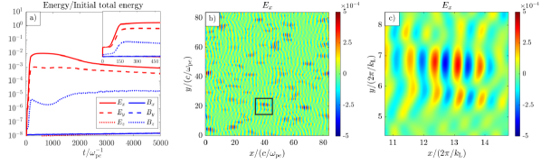
In Fig. 1 (panel a) we show the time history of the volume-averaged energy in each component of the electric and magnetic field ( and , respectively). The system’s evolution is divided in two distinct phases: during (blow-up inset in panel a), we observe the development of the initial electrostatic beam-plasma instability, which feeds off the input beam energy reservoir. This phase corresponds to the excitation of Langmuir waves666Note that during this initial phase, also grows in energy simply as a result of the beam-plasma instability without yet developing coherent electromagnetic waves at multiples of . appearing in the spatial distribution of the electrostatic field , shown at in panel b of the same Figure. Spatial fluctuations in can be observed throughout the domain; their wavelength is compatible with (where ), which identifies them as modes.
Mode conversion of forward-propagating waves occurs between and : in Fig. 2 (panel a with a zoomed-in view in panel d), we observe the presence, at , of spatial fluctuations in the ion density corresponding to the IAW wavelength (where ); simultaneously, the electromagnetic (out-of-plane) field develops coherent fluctuations that can be observed (panel b with a zoomed-in view in panel e) to be compatible with the wavelength of harmonic emission (where ). Moreover, filtering out high-frequency waves reveals underlying wave structures: by removing spectral modes with , the filtered field (panel c and cut-in view in panel f) shows large-scale fluctuations that can be identified as modes.
Our results provide one among the few clear, direct identifications of waves produced via fundamental and harmonic emission in a fully kinetic simulation of beam-plasma interaction. The detection of these modes confirms that the criteria outlined in Section 2 produce the expected three-wave mechanism efficiently, accurately capturing the dynamics of the corresponding mode conversion. During the development of this work, Zhang et al. (2022) also showed a similar result, and the analysis presented here broadly agrees with theirs. In the following Sections, we significantly expand this investigation by analyzing more quantitatively the development of all waves involved in the plasma-emission process and the dependence on the physical parameters employed.
3.2 Reference Run: Spectral Power in the Three-wave Modes
In Fig. 3 we show the spectral analysis of the modes of interest for the reference run. Panels a and b show the isotropic (i.e. cylindrically integrated in the -plane, via ) space-time FFT of the electrostatic at . The integration is performed separately for forward- () and backward-propagating () fluctuations, in order to diagnose counterpropagating and modes respectively. The cyan diamond in these plots indicates the phase-space location of the mode at the intersection of the Langmuir dispersion curve (orange line) with the beam dispersion curve (green line). Panel c similarly shows the isotropic space-time FFT of the magnetic field for , with the location of modes indicated by cyan diamonds along the plasma dispersion curve (red line). The spectral power in electrostatic and electromagnetic modes along the corresponding dispersion curves is shown at subsequent times in panels d, e, and f; in all cases, the spectra are clearly peaked around the wavenumbers of the modes involved in the three-wave interaction (dashed vertical lines), i.e. , , and , with the power in each mode increasing over time before stabilizing around a saturated value.
Interestingly, we note that an additional peak of spectral power arises at along the plasma dispersion curve. This “third-harmonic” emission () is weaker than both harmonic and fundamental signals, but it is clearly detectable as a byproduct of the three-wave interaction process, as we will demonstrate later. Higher-harmonic emission has been previously studied in fully kinetic simulations with a single parameter set (e.g. Rhee et al. 2009; Krafft & Savoini 2022b). We discuss this third-harmonic emission process more extensively in the next Sections.
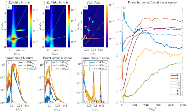
The evolution in time of the peak power in each mode of interest (measured at the corresponding ), including modes from ion-density fluctuations, is plotted in panel g of Fig. 3. We can observe that the evolution of the peak power in the forward-propagating modes is clearly correlated with the energetics of the primary beam-plasma instability that jumpstarts the plasma-emission process: power in the waves sharply rises within the first , reaching a maximum immediately followed by a slower decrease. During this time, modes also gain power as ion-density fluctuations develop. The subsequent dynamics builds on the nonlinear stage of the primary beam-plasma mode: power in modes decreases and backward-propagating modes develop together with , , and modes, reaching saturated values at . This is a clear indication that, at the very least, the process is actively pumping energy from the electrostatic modes into electromagnetic radiation. The resulting harmonic emission saturates at of the initial beam energy. In terms of fundamental emission, we observe that modes also steadily gain power and saturate over the same time scales of harmonic emission, but reach considerably lower saturation levels. This suggests that the conversion of electrostatic fluctuations into large-scale waves is less efficient, with the latter reaching saturation at around of the initial beam energy.
Finally, measuring the power deposited into third-harmonic electromagnetic waves reveals that modes also gain power and saturate, although over longer time scales and at much smaller energies than all other modes. Third-harmonic modes indeed receive only a small () fraction of the initial beam energy, which is however sufficient to clearly distinguish emission from the background noise. In the next Sections, we will show that in all our experiments third-harmonic waves invariably arise.
3.3 Effect of Density Ratio
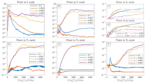
Fig. 4 shows the comparison of spectral power in the different modes (including ) over time, for variable initial beam-to-background density ratios (with for the reference simulation; all other parameters are kept fixed across runs, see Table 1). For each run, time is scaled by a factor to account for the different time scales of the beam-plasma instability that initiates the system’s evolution. As discussed in the previous sections, a large density ratio is expected not to result in the production of a strong signal due to the violation of matching conditions. Here, we explicitly observe the suppression of electromagnetic-wave production as decreases.
While the production of waves (panel a) by the initial beam-plasma instability is detected in all cases (albeit with different dynamics for large ), we observe that for the subsequent three-wave interaction is not triggered. Indeed, we measure significant power in backward-propagating waves (see panel b) only when , even though IAWs are developing in all runs (panels c1 and c2). The presence of counterpropagating waves at wavenumbers satisfying the three-wave interaction conditions is in principle sufficient to ensure that emission occurs; we indeed observe growth and saturation of power in for the cases, and no such dynamics for larger density ratios (panel e). Similarly, a clear, saturated signal (roughly 100 times weaker than the signal) develops for the low-density runs (panel e). emission was not detected clearly in some previous works, particularly when the system size was not taken large enough to fit wavelengths (Thurgood & Tsiklauri 2015; see Section 2).
Our results provide a definitive confirmation that both fundamental and harmonic plasma emission can occur as a consequence of a simple beam-plasma interaction; but to observe this mechanism in simulations, it is necessary to perform large calculations of sufficient size and with sufficiently low beam-plasma density ratio. Power in the harmonic emission appears to asymptotically (for small enough ) saturate and converge to a fraction () of the initial beam energy; power in the fundamental emission saturates to energies roughly 100 times smaller. The fact that harmonic and fundamental emission do not occur for large , even though technically all basic ingredients ( and waves) are present, is likely due to the violation in the matching conditions introduced in Section 1. This will be further discussed in Section 5.
Finally, we quantitatively confirm the presence of a third-harmonic emission type in Fig. 4 (panel f). Power in waves clearly rises and saturates similarly to that of other electromagnetic modes, although with a visible delay and at significantly lower power levels. It is interesting to note that this third-harmonic emission only appears with a sufficiently low , suggesting that the mechanism for production may require conditions similar to those allowing harmonic and fundamental emission. We will discuss such mechanisms in Section 5.
4 Dependence of plasma emission on temperature ratio
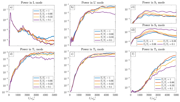
We conclude our parameter-space exploration by comparing the reference run from Table 1 () with a series of runs where we vary . The results are shown in Fig. 5, again in terms of the spectral power in individual modes measured at the corresponding locations from the cylindrically integrated FFTs of the field quantities.
Qualitatively, we observe no drastic change in the system’s evolution as the ion-to-electron temperature ratio varies between 0.1 and 1: the reference run attains saturated power levels in and waves moderately lower than the other runs (up to a factor ), but overall we observe growth and saturation of power in all modes. The only notable difference arises in the evolution of IAWs (panels c1 and c2 in Fig. 5): for the reference run, we observe the power in modes growing and saturating, while for the other runs we only see an initial growth in spectral power followed by a steady decay. This is a signature that the production of IAWs is much less efficient for large temperature ratios, due to strong Landau damping, in accordance with linear theory (Fried & Gould 1961). It is then rather counterintuitive that the production of modes (panel b), and thus of fundamental and harmonic emission (panels d and e), remains active even when waves are scarcely excited. We also notice that the growth rate of the power in modes during is different for runs with different , and is larger when the temperature ratio is smaller. In runs with large , the creation of waves can be explained by the direct backscattering of waves off moving ions (e.g. Tsytovich & Kaplan 1969; Zlotnik et al. 1998), which is a fundamentally different phenomenon from the collision of with waves that can occur when the temperature ratio is small. We discuss this aspect more in detail in Section 5.
We conclude by noting that also for this parameter-space exploration we invariably measure a clear growth in the power associated with modes. This supports the idea that third-harmonic emission occurs under the same conditions that allow for harmonic and fundamental modes, regardless of the presence (or absence) of saturated modes.
5 Discussion and conclusions
In this Letter, we presented conclusive evidence for the efficient production of fundamental and harmonic plasma emission ( and waves) in fully kinetic simulations of beam-plasma interactions. By performing an array of runs with different initial parameters, we observed that harmonic emission saturates asymptotically to of the initial beam energy, while fundamental emission is roughly 100 times weaker. The emission process broadly aligns with theoretical expectations — i.e., it is only detected when the beam-to-background density ratio (as well as the energy ratio ) is sufficiently small — but a few of our key results are novel and require further discussion.
First, our series of simulations with variable density ratio shows that, in all cases (also for large ), Langmuir () and ion acoustic () waves are produced from the precursor electrostatic instability excited by our initial conditions. According to linear theory, and modes are in principle the building blocks for the production of backward-propagating (at first) and (as a second-order effect) waves, and thus it is not obvious why plasma emission would not occur when (i.e. the beam energy is of the background energy). As shown by Cairns 1989, when the power in modes peaks at a frequency significantly below () that of the Langmuir dispersion curve. As a consequence, matching conditions in the frequency allowing for the interaction of and waves are broken ( modes do not exist at frequencies that can compensate the mismatch) and backward-propagating electrostatic modes are not produced, inhibiting the subsequent plasma emission. This fact was also considered by Thurgood & Tsiklauri (2015) and Zhang et al. (2022), and we now provide solid evidence for its occurrence in a series of runs where varies by two orders of magnitude. In our runs (relatively close to the limit calculated by Cairns 1989), modes firmly sit on the Langmuir dispersion curve and matching conditions are met, allowing for plasma emission.
A second point requiring clarification concerns our runs with variable . In all these simulations, plasma emission is invariably detected, even though IAWs are less efficiently produced for , preventing the interaction of and waves that results in and then waves. The fact that across all runs (even for ) we measure comparable saturated power levels for and modes can thus be explained by considering direct backscattering off moving ions. In the absence of waves, a forward-propagating wave can directly collide with an ion moving in the opposite direction (e.g. Tsytovich & Kaplan 1969): the electrostatic wave interacts with the surrounding cloud of electrons, which reemits the wave while transferring momentum to the ion. This causes a recoil in the ion motion and the emission of a backward-propagating wave. Although further work is required to provide more evidence linking our simulations with this mechanism, these results firmly establish that plasma emission is essentially insensitive of the ion-to-electron temperature ratio, and is instead uniquely dependent on the beam-to-background energy ratio (in our study, expressed by the density ratio). This is in contrast with previous multidimensional simulation studies where values were assumed to produce no plasma emission. We note that analytic works and one-dimensional simulations (e.g. Rha et al. 2013 and references therein) have mentioned the possibility of producing plasma emission at due to highly efficient ion scattering compensating for the lack of interaction with waves.
As an additional result, we emphasize that in all our runs where plasma emission occurs we also invariably detected a clear, peaked signal at , indicating the presence of third-harmonic modes along the plasma dispersion curve. Analytic calculations have suggested that interactions occurring as a byproduct of harmonic emission can give rise to this third-harmonic signal (e.g. Zlotnik et al. 1998); a second possibility is the direct coalescence of multiple electrostatic modes, i.e. (Kliem et al. 1992). However, the latter is more likely for slow electron beams coupled with strong electron density gradients (Yi et al. 2007), which does not correspond to the conditions of our simulations. Higher-harmonic plasma emission has been observed in the past in PIC simulations (in the case of a homogeneous-density background which we employ) considering a single set of parameters: Rhee et al. (2009) and Krafft & Savoini (2022b) have reported the detection of third-harmonic (and higher) emission, relating it to the Zlotnik et al. (1998) mechanism of coalescence. Our array of runs explores a broad range of simulation parameters (in terms of beam-to-background density and ion-to-electron temperature ratios) with uniform background density, where we detected third-harmonic emission in all cases where emission occurred. Our results thus appear to support the hypothesis, implying that the growth of third-harmonic modes may be feeding off the harmonic emission process. The power we measure in third-harmonic emission is roughly 100–1000 times smaller than the power in harmonic modes, which appears to align with observations of Type II (e.g. Kliem et al. 1992; Zlotnik et al. 1998) and III (e.g. Takakura & Yousef 1974; Reiner & MacDowall 2019) radio bursts; still, a broader array of data (numerical and experimental) would be required to firmly establish this correspondence. Even though more in-depth investigation is needed, our results provide the unambiguous direct detection of third-harmonic plasma emission in a large array of kinetic simulations of beam-plasma interaction which explore very different parameter regimes. This allows us to claim that third-harmonic emission could be an invariable byproduct of the three-wave-interaction process even when physical conditions vary considerably.
Our work demonstrates efficient production of coherent emission in a relatively simple setting where a single beam interacts with a uniform background, leaving ample ground for further developments. In particular, it would be important to consider the effect of background magnetic fields and/or density inhomogeneities, as well as the presence of counterstreaming beams (Tsiklauri 2011; Thurgood & Tsiklauri 2015, 2016; Lazar et al. 2023). Furthermore, it is known that the emission efficiency for different modes can have strong dependence on other parameters such as heliocentric distance, background-wind speed, and ambient-density fluctuations (e.g. Robinson & Cairns 1998a, b, c; Voshchepynets et al. 2015; Krafft & Savoini 2021, 2022a). Another possibility is the production of plasma emission without three-wave interaction when a magnetized electron beam encounters a density shear (e.g. Schmitz & Tsiklauri 2013). In all these cases, a rigorous parameter-space exploration akin to the one performed here would reveal under which conditions coherent emission can be expected, relating directly to various astrophysical scenarios where electron beams are present, such as coronal loops, shock waves from coronal mass ejections, etc.
Acknowledgements
F.B. would like to thank Immanuel Christopher Jebaraj and Marian Lazar for useful discussions and suggestions throughout the development of this project. F.B. acknowledges support from the FED-tWIN programme (profile Prf-2020-004, project “ENERGY”) issued by BELSPO, and from the FWO Junior Research Project G020224N granted by the Research Foundation – Flanders (FWO). The simulations were performed on the NSF Frontera supercomputer (Stanzione et al., 2020) at the Texas Advanced Computing Center (TACC, www.tacc.utexas.edu) under grant AST21006, and at the VSC (Flemish Supercomputer Center), funded by the Research Foundation Flanders (FWO) and the Flemish Government – department EWI. This work was performed in part at Aspen Center for Physics, which is supported by National Science Foundation grant PHY-1607611.
Data Availability
The data underlying this article will be shared on reasonable request to the corresponding author.
References
- Buneman (1993) Buneman O., 1993, Computer Space Plasma Physics. Tokyo: Terra Scientific
- Cairns (1989) Cairns I. H., 1989, Physics of Fluids B: Plasma Physics, 1, 204
- Cairns & Robinson (1998) Cairns I. H., Robinson P. A., 1998, ApJ, 509, 1
- Dulk (1985) Dulk G. A., 1985, Annual Review of Astronomy and Astrophysics, 23, 1
- Fried & Gould (1961) Fried B. D., Gould R. W., 1961, The Physics of Fluids, 4, 139
- Ginzburg & Zhelezniakov (1958) Ginzburg V. L., Zhelezniakov V. V., 1958, Soviet Ast., 2, 653
- Hakobyan et al. (2023) Hakobyan H., Spitkovsky A., Chernoglazov A., Philippov A., Groselj D., Mahlmann J., 2023, PrincetonUniversity/tristan-mp-v2: v2.6, doi:10.5281/zenodo.7566725, https://doi.org/10.5281/zenodo.7566725
- Henri et al. (2019) Henri P., Sgattoni A., Briand C., Amiranoff F., Riconda C., 2019, Journal of Geophysical Research: Space Physics, 124, 3
- Kasaba et al. (2001) Kasaba Y., Matsumoto H., Omura Y., 2001, Journal of Geophysical Research: Space Physics, 106, A9
- Kliem et al. (1992) Kliem B., Krüger A., Treumann R. A., 1992, Solar Physics, 140, 149
- Krafft & Savoini (2021) Krafft C., Savoini P., 2021, ApJL, 917, L23
- Krafft & Savoini (2022a) Krafft C., Savoini P., 2022a, ApJL, 924, L24
- Krafft & Savoini (2022b) Krafft C., Savoini P., 2022b, ApJL, 934, L28
- Lazar et al. (2023) Lazar M., López R. A., Poedts S., Shaaban S. M., 2023, Solar Physics, 298, 72
- Lee et al. (2019) Lee S.-Y., Ziebell L. F., Yoon P. H., Gaelzer R., Lee E. S., 2019, ApJ, 871, 74
- Lee et al. (2022) Lee S.-Y., Yoon P. H., Lee E., Tu W., 2022, ApJ, 622, L157
- Marquès et al. (2020) Marquès J.-R., et al., 2020, Phys. Rev. Lett., 124, 135001
- Melrose (1970a) Melrose D. B., 1970a, Australian Journal of Physics, 23, 885
- Melrose (1970b) Melrose D. B., 1970b, Australian Journal of Physics, 23, 871
- Melrose (2017) Melrose D. B., 2017, Rev. Mod. Plasma Phys., 1
- Ndacyayisenga et al. (2023) Ndacyayisenga T., Uwamahoro J., Uwamahoro J. C., Babatunde R., Okoh D., Sasikumar Raja K., Kwisanga C., Monstein C., 2023, EGUsphere, 2023, 1
- O’Neil & Malmberg (1968) O’Neil T. M., Malmberg J. H., 1968, Physics of Fluids, 11, 1754
- Reid & Ratcliffe (2014) Reid H. A. S., Ratcliffe H., 2014, Research in Astronomy and Astrophysics, 14, 773
- Reiner & MacDowall (2019) Reiner M. J., MacDowall R., 2019, Solar Physics, 294, 91
- Rha et al. (2013) Rha K., Ryu C.-M., Yoon P. H., 2013, The Astrophysical Journal Letters, 775
- Rhee et al. (2009) Rhee T., Ryu C.-M., Woo M., Kaang H. H., Yi S., Yoon P. H., 2009, ApJ, 694, 618
- Robinson & Cairns (1998a) Robinson P. A., Cairns I. H., 1998a, Solar Physics, 181, 363
- Robinson & Cairns (1998b) Robinson P. A., Cairns I. H., 1998b, Solar Physics, 181, 395
- Robinson & Cairns (1998c) Robinson P. A., Cairns I. H., 1998c, Solar Physics, 181, 429
- Sakai et al. (2005) Sakai J. I., Kitamoto T., Saito S., 2005, ApJ, 622, L157
- Schmitz & Tsiklauri (2013) Schmitz H., Tsiklauri D., 2013, Physics of Plasmas, 20, 062903
- Spitkovsky (2005) Spitkovsky A., 2005, in Bulik T., Rudak B., Madejski G., eds, American Institute of Physics Conference Series Vol. 801, Astrophysical Sources of High Energy Particles and Radiation. pp 345–350
- Stanislavsky et al. (2022) Stanislavsky A. A., Bubnov I. N., Koval A. A., Yerin S. N., 2022, A&A, 657, A21
- Stanzione et al. (2020) Stanzione D., West J., Evans R. T., Minyard T., Ghattas O., Panda D. K., 2020, Frontera: The Evolution of Leadership Computing at the National Science Foundation. Association for Computing Machinery, New York, NY, USA, p. 106–111, https://doi.org/10.1145/3311790.3396656
- Sydora (2003) Sydora R. D., 2003, Low Noise Electrostatic and Electromagnetic Delta-f Particle-in-Cell Simulation of Plasmas. Springer Berlin Heidelberg, Berlin, Heidelberg, pp 109–124
- Takakura & Yousef (1974) Takakura T., Yousef S., 1974, Solar Physics, 36, 451
- Thurgood & Tsiklauri (2015) Thurgood J. O., Tsiklauri D., 2015, A&A, 584, A83
- Thurgood & Tsiklauri (2016) Thurgood J. O., Tsiklauri D., 2016, JPP, 82, 905820604
- Tsiklauri (2011) Tsiklauri D., 2011, PoP, 18, 052903
- Tsytovich (1972) Tsytovich V. N., 1972, An introduction to the theory of plasma turbulence.. Pergamon
- Tsytovich & Kaplan (1969) Tsytovich V. N., Kaplan S. A., 1969, Soviet Astronomy, 12, 618
- Umeda (2010) Umeda T., 2010, JGR, 115, A01204
- Voshchepynets et al. (2015) Voshchepynets A., Krasnoselskikh V., Artemyev A., Volokitin A., 2015, ApJ, 807, 38
- Wild & Smerd (1972) Wild J. P., Smerd S. F., 1972, Annual Review of Astronomy and Astrophysics, 10, 159
- Yi et al. (2007) Yi S., Yoon P. H., Ryu C.-M., 2007, PoP, 14, 013301
- Zhang et al. (2022) Zhang Z., Chen Y., Ni S., Li C., Ning H., Li Y., Kong X., 2022, ApJ, 939, 63
- Zheleznyakov & Zaitsev (1970) Zheleznyakov V. V., Zaitsev V. V., 1970, Soviet Ast., 14, 47
- Zlotnik et al. (1998) Zlotnik E. Y., Klassen A., Klein K.-L., Aurass H., Mann G., 1998, A&A, 331, 1087